a divergence-free multidomain spectral solver of …rpas/publis/jcp98.pdfjournal of computational...

JOURNAL OF COMPUTATIONAL PHYSICS139,359–379 (1998)ARTICLE NO. CP975875

A Divergence-Free Multidomain SpectralSolver of the Navier–Stokes Equations

in Geometries of High Aspect Ratio

C. Sabbah and R. Pasquetti

Laboratoire J.A. Dieudonne, UMR CNRS N◦6621, Universite de Nice Sophia-Antipolis,Parc Valrose, Nice Cedex 2, 06108, France

E-mail: rpas@math. unice.fr

Received February 3, 1997; revised September 25, 1997

In order to solve with high accuracy the incompressible Navier-Stokes equationsin geometries of high aspect ratio, one has developed a spectral multidomain algo-rithm, well adapted to the parallel computing. In cases of 2D problems, a Chebyshevcollocation method and an extended influence matrix-technique are used in each sub-domain, to solve the generalized Stokes problem which results from the discretizationin time. The continuity conditions, needed at the interfaces of each subdomain, arecomputed by using again an influence matrix, the setup of which ensures all thenecessary compatibility conditions, especially the incompressibility. This work isalso described for 3D problems with one homogeneous direction. A study of accu-racy versus the number of subdomains is presented, as well as an example of anapplication concerned with Rayleigh–B´enard convection in a cavity of large aspectratio. c© 1998 Academic Press

1. INTRODUCTION

Some physical problems require the accurate solution of the incompressible Navier–Stokes equations in geometries of high aspect ratio. As a matter of example, double diffusiveconvection in a tank of great height can be affected with instabilities that do not occur if theheight is not large enough. Another problem of interest that requires such kinds of geometriesis the study of the spatial development of wakes behind an obstacle. To this aim, we firstdeveloped a 2D Chebyshev multidomain parallel solver and this work was extended to thetreatment of 3D geometries with one homogeneous direction. The multidomain approachis implemented along the direction of great length.

As it is well known, many approaches are possible for the approximation of the Navier–Stokes equations. Especially, one can use the so-calledprojection methods, as e.g. de-scribed in [1–4], or the two steps method described in [5], when restricting ourselves to the

359

0021-9991/98 $25.00Copyright c© 1998 by Academic Press

All rights of reproduction in any form reserved.

360 SABBAH AND PASQUETTI

Chebyshev (or Legendre) spectral methods. Nevertheless, such approaches are often usedto bypass the so-called generalized Stokes problem (GSP) which naturally results from theunsteady Stokes or Navier–Stokes equations, when using in time a finite difference schemetreating more or less implicitly the linear diffusion term and explicitly the nonlinear one,as generally done with spectral methods. Indeed, in nonperiodic geometries, solving theGSP is not a trivial task. Especially, approaches based on the direct solution of the so-calledUzawa operator to compute the pressure are generally not realistic, owing to memory stor-age requirements. This is the reason why iterative procedures are usually preferred, as e.g.in [6, 7], but the obtention of a satisfactory convergence rate is not straightforward.Themonodomain GSP solver used in this work is briefly described in Section 2. It makes useof a spectral collocation method (see, e.g. [8]) based on an “extended influence matrix”technique, yielding the pressure, as well as the collocation error at the boundary, as firstdescribed in [9, 10]. The main advantage of such an approach is the obtention of the exactsolution of the discrete form of the GSP, when its main drawback lays in its memory stor-age requirement. Moreover, owing to the use of the same grids and same polynomial vectorspaces for the approximations of the velocity components and of the pressure, the latter isaffected with spurious modes, as e.g. mentioned in [11]. For this reason, we also describein Section 2 an algorithm to recover (when necessary) the pressure in a satisfactory way.

The multidomain procedure is considered is Section 3. Essentially, it is a nonoverlapping,patching, and direct method (based on an influence matrix technique) that is used forthe computation of the velocity at the interfaces of the subdomains [8]. Once knowingthe velocity at the boundary of each subdomain, one uses the monodomain GSP solverin each and finally derives the complete velocity field. As usual with patching methods,the continuity of the velocity at the interfaces is enforced strongly, as e.g. in [12] or in[13] (where an overlapping procedure is used). Such patching approaches differ from thevariational approaches which generally only require theC0 continuity of the velocity (see,e.g. [14, 15]). The method is direct, since it uses an influence matrix technique to computethe interface values (as in [12], where only one direction is nonhomogeneous). Such directapproaches are very efficient, but clearly require a sufficiently small number of interfacecollocation points. In other contexts, iterative procedures become necessary (as, e.g. in[16, 14]). In the framework of the vorticity-stream function formulation of the 2D Navier–Stokes equations, the use of an influence matrix technique is also suggested in [17–19].But when using the velocity–pressure formulation the setup of this matrix is more complex,owing to the incompressibility constraint. In our approach compatibility conditions mustbe considered to preserve the main property of the monodomain solver, the divergence-freefeature of the computed velocity. The approach makes intensive use of this property andutilizes original bases for spanning the interface velocity components.

The last section of this paper presents numerical results obtained on a CRAY T3D (orT3E) supercomputer. First, a study of accuracy is done by considering a GSP for whichan analytical solution is known. Then we show the results of the numerical experimentsconcerned with 2D and 3D Rayleigh–B´enard convection in a cavity of aspect ratio equal to 8.

2. MONODOMAIN ALGORITHM

Let us consider the incompressible Navier–Stokes equations in a rectangular domainÄ

of boundary0 and assume admissible Dirichlet boundary conditions for the velocity. When

MULTIDOMAIN SPECTRAL SOLVER 361

using in time an implicit (or semi-implicit) approximation of the diffusion term and anexplicit one for the convection term, at each time step the GSP

1V − σV = ∇ p+ f in Ä (1)

∇ · V = 0 in Ä (2)

V|0 = V0 (3)

has to be solved, withÄ for the closure ofÄ and whereV stands for the velocity,p is for thepressure times the Reynolds number, andf is for a given body force term. The parameterσ is proportional to the ratio of the Reynolds number to the time step and depends on thescheme used for the discretization.

2.1. “Extended Influence Matrix” Technique

As is well known, as soon as the pressure and the body-force term are smooth enough,the problem (1)–(3) is equivalent to

1V − σV = ∇ p+ f in Ä (4)

1p+∇ · f = 0 inÄ (5)

∇ · V|0 = 0 (6)

V|0 = V0. (7)

Then the difficulty comes from the fact that no boundary conditions are available forthe pressure. But this difficulty can be overcome by splitting the problem (4)–(7) into twoproblems [20],

1V1− σV1 = ∇ p1+ f in Ä (8)

1p1+∇ · f = 0 inÄ (9)

p1|0 = 0 (10)

V1|0 = V0 (11)

and

1V2− σV2 = ∇ p2 in Ä (12)

1p2 = 0 inÄ (13)

p2|0 =M−1(−∇ · V1|0

)(14)

V2|0 = 0 (15)

whereM is an “influence operator” defined by

Mp2|0 = ∇ · V2|0 (16)


in such a way that

∇ · V1|0 +∇ · V2|0 = ∇ · V|0 = 0. (17)

In Eq. (14)M−1 is a generalized inverse of the operatorM, since the pressure can onlybe defined up to a constant. After discretization, the operatorM is the so-called influencematrix. It is built during a preliminary calculation, by solving a set of elementary problemssimilar to the problem (12)–(15), but withp2|0 given. Thus, when using a collocationmethod, the boundary values ofp2 are successively taken as unitary at the different boundarynodes to constitute the different columns of the influence matrix.

Such a splitting approach partially fails in the sense that the resulting velocity field isnot perfectly divergence-free. Since [9, 10] this failure is well understood, the momentumequation (4) being not collocated at the boundary, the body force term of the Poissonequation (5) is polluted by an extra term that prevents from obtaining the desired result.Moreover, as shown in [10], where the tau method (see, e.g. [8]) is also investigated, thisfailure is not specific to the collocation method.

In order to outline this point and to briefly present the “extended influence matrix tech-nique” (see [21] for an extensive presentation), let us assume thatÄ= ]−1, 1[2 (using amapping if necessary) and introduce the(I +1)× (J+1)Gauss–Lobatto mesh associatedwith the Chebyshev polynomials:

ÄI ,J ={

cos

(π i

I

), cos

(π j

J

)}, 0≤ i ≤ I ; 0≤ j ≤ J, (18)

ÄI ,J ={

cos

(π i

I

), cos

(π j

J

)}, 0< i < I ; 0< j < J, (19)

0I ,J = ÄI ,J\ÄI ,J . (20)

Then, withPI ,J the vector space of the polynomials of maximum degreeI in x and J iny, the Chebyshev collocation method consists in findingV in (PI ,J)

2 and p in PI ,J suchas

1V − σV = ∇ p+ f in ÄI ,J (21)

∇ · V = 0 in ÄI ,J (22)

V|0I ,J = V0I ,J . (23)

Here we notice that Eq. (22) implies thatV is perfectly divergence-free, since a poly-nomial in PI ,J which vanishes at(I + 1)(J + 1) collocation points is the null polyno-mial. Moreover, the boundary condition (23) is assumed admissible; i.e, the polynomialinterpolants ofV0|0I ,J at each side ofÄ are compatible with the incompressibility con-straint.

In order to take into account the error that occurs in the momentum equation, let us nowintroduce an additive unknown termτ , in (PI ,J)

2 such that

τ = 0 in ÄI ,J (24)


and rewrite the following new version of system (4)–(7):

1V − σV = ∇ p+ f + τ in ÄI ,J (25)

1p+∇ · f +∇ · τ = 0 inÄI ,J (26)

∇ · V|0I ,J = 0 (27)

V|0I ,J = V0I ,J . (28)

The “extended influence matrix” algorithm is based on the splitting of problem (25)–(28),

1V1− σV1 = ∇ p1+ f + τ 1 in ÄI ,J (29)

1p1+1 · f = 0 inÄI ,J (30)

p1|0I ,J = 0 (31)

V1|0I ,J = V0I ,J (32)

and

1V2− σV2 = ∇ p2+ τ + τ 2 in ÄI ,J (33)

1p2+∇ · τ = 0 inÄI ,J (34)

{p2|0I ,J , τ |0I ,J } =M−1{−∇ · V1|0I ,J ,−τ 1|0I ,J } (35)

V2|0I ,J = 0, (36)

whereτ 1 andτ 2 are the collocation errors which occur at the boundary nodes, where themomentum equations are not enforced (N.B.,τ 1 andτ 2 can only be computeda posteriori).M is now an influence matrix (andM−1 is a generalized inverse) defined by

M{p2|0I ,J , τ |0I ,J } = {∇ · V2|0I ,J , τ2|0I ,J } (37)

in such a way that

∇ · V1|0I ,J +∇ · V2|0I ,J = ∇ · V|0I ,J = 0 (38)

τ 1|0I ,J + τ 2|0I ,J = 0. (39)

As presented here the dimension of the influence matrixM appears to be very large. But,in fact, this dimension can be drastically decreased because it is only the normal componentof τ that is required to compute∇ · τ in ÄI ,J . If we denote byτ the normal componant(to the boundary) ofτ and if we consider thatp2|0I ,J = p|0I ,J , then the influence matrixeffectively involved in the computation is such that

M{p|0I ,J , τ |0I ,J } = {∇ · V2|0I ,J , τ2|0I ,J }. (40)

Moreover, the collocation method does not need the values ofp andτ at the four cornersof the domain and so it only needs these values at 2(I + J − 2) boundary nodes. The


dimension of the extended influence matrix is then 4(I + J − 2), i.e. twice larger than theusual influence matrix. It can be set up in a preliminary calculation by solving the elementaryproblems associated with the canonical basis of the vector spaceR4(I+J−2) for the boundarynode values ofp2 andτ in Eqs. (33) and (34). Once the influence matrix is calculated, onehas to invert it, but as outlined later in the text one has a rank deficiency equal to four.One way to proceed is to compute the eigenvalues and then replace the four zero valuesby nonnull values, in order to project the solution onto the orthogonal complement of thekernel. Contrary to what is mentioned in [22], where one suggests using infinite values, thenonnull values can be arbitrary, without any incidence onp|0I ,J andτ |0I ,J .

Finally, the algorithm is the following:

—solve the problem (29)–(32) and, once knowing the velocity and pressure fieldsV1

and p1, compute the values of∇ · V1|0I ,J andτ 1|0I ,J ;—from Eq. (35) compute the boundary values of the pressurep|0I ,J and of the correction

termτ |0I ,J ;—solve the problem (25)–(28) using the prescribed values ofp|0I ,J andτ |0I ,J .

Remark. The initial problem (21)–(23) only requires the knowledge off inÄI ,J , on thecontrary of the approach, based on the standard influence matrix technique. This propertyis recovered when using the extended influence matrix approach, since the error termτ

permits us to assume arbitrary values off at the the boundary nodes. Thus, one can simplyassumef |0I ,J = 0.

2.2. Calculation of the Pressure

The advantage of assumingp in PI ,J is that a divergence-free velocity fieldV can effec-tively be produced, but this advantage goes with the drawback that the pressure is affectedwith spurious modes [23]. WithTi (x) = cosi (cos−1 x) for the Chebyshev polynomial ofdegreei , these spurious modes are:

—the constant modeT0(x)T0(y) = 1, which is physical, since the pressure is defined upto a constant,

—the column modeTI (x)T0(y) = TI (x),—the line modeT0(x)TJ(y) = TJ(y),—the checkerboard modeTI (x)TJ(y).

The nonphysical spurious modes result from the definition of the Gauss–Lobatto mesh(Eq. (18)) for which(1−x2)(1−y2)T ′I (x)T

′J(y) = 0 (with a prime for the first-order deriva-

tive). Moreover, since the corner values of the pressure are not required by the algorithmso they can be arbitrary, one has also:

—the four corner modes.

In the framework of the “extended influence matrix technique” the spurious modes ofpressure are associated with spurious modes ofτ . Indeed, from Eqs. (25) and (26), it isclear that the spurious partspsp andτ sp of p andτ verify the set of equations [22]:

∇ psp+ τ sp = 0 in ÄI ,J (41)

τ sp|ÄI ,J = 0 (42)

1psp+∇ · τ sp = 0 inÄI ,J . (43)


Then,

—τ sp= (0, 0),—τ sp= (−T ′I (x), 0),—τ sp= (0,−T ′J(y)), and—τ sp= (−T ′I (x)TJ(y),−TI (x)T ′J(y))

are respectively associated with the constant, column, line, and checkerboard modes. Therestictions to the boundary of these four spurious couples constitute a basis of the influ-ence matrix kernel. Consequently,M has a rank deficiency equal to four, as mentioned inSection 2.1.

Remark. When using the standard influence matrix approach, the Poisson equation (43)for psp becomes homogeneous and is no longer verified by the nonphysical spurious modes.The dimension of the kernel of the standard influence matrix then equals one.

How can we recover the pressure field? The natural idea is to filter the nonphysical modes,but more problematic is the question of the corner modes, since vanishing the pressure atthe four corners of the domain is clearly not physical. Let us first assume that the valuespl , 1 ≤ l ≤ 4, of the pressure at the corners are known. Then, in the Chebyshev spectralspace the spurious modes can be cancelled, in order to get the filtered pressure fieldp′,which depends on thepl . The natural idea is then to produce a smooth pressure field. Thiscan be achieved by solving the following optimization problem: find thepl such that thefunctional

J(pl ) =∑ÄI ,J

|∇ p′|2 (44)

is minimal. But inÄI ,J the gradient of the pressure does not depend on the pressure spuriousmodes, so that the functional can be rewritten in the simpler form,

J(pl ) =∑0I ,J

|∇ p′|2. (45)

This optimization problem can be easily solved after noticing thatp can read

p = p0+∑

l

pl Cl , (46)

wherep0 is the initial pressure field with zero values at the corners and where theCl arethe polynomials which vanish everywhere inÄI ,J , except at the corners where they takeunitary values. After filtering the four spurious modes one gets

p′ = p′0+∑

l

pl C′l , (47)

∇ p′ = ∇ p′0+∑

l

pl∇C′l , (48)

where the∇C′l vanish inÄI ,J . It is then easy to express∇ p′|0I ,J in terms of thepl and tocompute thesepl by using a standard least square method.


2.3. Extension to 3D Geometries with One Homogeneous Direction

When assuming that thez direction is homogeneous a discrete Fourier expansion of thedifferent variables can be used along this direction. Then, the 3D problem decouples intoa set of 2D complex problems. Namely, for each mode numberk, 0 ≤ k ≤ K , one getsthe following system of equations that must solve the Fourier spectra (denoted by ˆ.k) of thedifferent variables,

1kVk − σVk = ∇k pk+ f k + τ k in ÄI ,J (49)

1k pk +∇k · f k +∇k · τ k = 0 (50)

∇k ·Vk|0I ,J = 0 (51)

Vk|0I ,J = Vk0I ,J , (52)

where1k = ∂xx + ∂yy − k2 and∇k = (∂x, ∂y, ik), with i for the square root of−1. Foreach mode number one can apply the extended influence matrix algorithm and thus obtaina set of influence matricesMk, such that

Mk{ pk|0I ,J ,τk|0I ,J } ={∇k ·V2

k|0I ,J , τ2k |0I ,J

}. (53)

These influence matricesMk are real; they associate the real (imaginary) parts of

{ pk|0I ,J , τk|0I ,J } to the real (imaginary) parts of{∇k · V2k|0I ,J , τ

2k |0I ,J }.

Finally, one has to mention that fork 6= 0, the influence matrices are regular. This resultsfrom the fact that ifpk does not vanish inÄI ,J , then∇k pk is also nonnull inÄI ,J . On thecontrary, ifk = 0 the 2D situation and the spurious modes of pressure are recovered.

3. MULTIDOMAIN APPROACH

In this section we present a multidomain approach, based on the use of the monodomainsolver which has just been presented, to solve the GSP with the no-slip boundary condition.First we begin with the 2D case, by considering for the domainÄ a rectangle of large aspectratio. This domainÄ is splitted, versus the direction of great length (x direction) into a setof N subdomainsÄn. The interface between the subdomainsÄn andÄn+1 is denoted byIn.At the intersections ofIn and of the boundary0 ofÄ, one has the pointsAn andBn in sucha way thatÄn, of boundary0n, is the squareAn−1, An, Bn, Bn−1. Moreover we assume theuse of matching grids: for alln, the number of collocation points between the pointsAn

andBn is equal to (J − 1).

3.1. Interface Conditions

With V = (u, v) and v · bn for the jump at the interfacesIn, the essential and naturalcontinuity conditions that the PDE (1) induces to use at these interfaces read:

vubn = vvbn = v∂xu− pbn = v∂xvbn = 0. (54)


Nevertheless, when taking into account that the velocity is divergence-free, the first, second,and fourth conditions imply thatu is C2-continuous:

v∂xubn + v∂yvbn = v∂xubn = 0 (55)

v∂xxubn + v∂xyvbn = v∂xxubn = 0. (56)

It results that in the case of incompressible fluids the interface conditions read:

vubn = vvbn = vpbn = v∂xvbn = 0. (57)

Let us go to the discrete framework. When using the approach described in Section 2, theprevious interface conditions should still hold, because the approximate velocity field isalso perfectly divergence-free. But the spurious modes of pressure prevent the use of thethird condition, i.e. the one involving the pressure jump.

In order to overcome this difficulty, we first tried to enforce theC2 continuity ofv ratherthan theC0 continuity of p, i.e. to substitute for the conditionvpbn= 0 the one,v∂xxvbn= 0.Such an approach is quite satisfactory for solving a GSP and even the nonstationary Navier–Stokes equations at low Reynolds numbers. Unfortunately, when the Reynolds number isincreased, oscillations of the solution generally occur at the interfacesIn and then amplify,until inducing numerical instability.

The way that we suggest and use now successfully, consists in a weak formulationof the interface conditionvpbn= 0. This permits us to overcome efficiently the problemof the spurious modes of pressure, without inducing any deterioration of the solution atthe interfacesIn. For the sake of clarity, this weak formulation of the pressure continuitycondition will be detailed in Subsection 3.3, after the description of the influence matrixtechnique that is used in our multidomain approach.

Remark. The interface conditions (57) induce theC0 continuity of the vorticity,ω = ∂xv − ∂yu.

3.2. Influence Matrix Technique

Let us split the GSP into two sets ofN monodomain problems,P1n andP2

n . For the firstset, one assumes for each subdomain homogeneous Dirichlet boundary conditions and onetakes into account the body-force term:

ProblemsP1n read:

1V1− σV1 = ∇ p1+ f in Än (58)

∇ · V1 = 0 in Än (59)

V1|0n = 0. (60)

Once this first set of problems is solved the jumpsvp1bn andv∂xv1bn can be computed.

For the second set of problems, one uses at the interfacesIn, 1≤ n≤ (N− 1), the nonho-mogeneous Dirichlet conditions(u2, v2)|In , which ensure the interface conditions, i.e. suchthat for alln,

vp1bn + vp2bn = 0 (61)


v∂xv1bn + v∂xv

2bn = 0. (62)

ProblemsP2n read:

1V2− σV2 = ∇ p2 in Än (63)

∇ · V2 = 0 in Än (64)

V2|0n = V0n . (65)

ThenV1+ V2 is the solution of the complete problem.Thanks again to the linearity property of the GSP, in order to determine the appropriate

values of(u2, v2)|In , in fact equal to(u, v)|In , a new influence matrixM can be introducedsuch that

M{∪(u, v)|In} = {∪(vp2bn, v∂xv2bn)} (66)

with ∪ for union overn (1≤ n ≤ (N − 1)).The influence matrixM is clearly block tridiagonal, since if the velocity is only nonnull

at the interfaceIn, then the jumpsvpbn andv∂xvbn are only nonnull at the interfacesIn, In+1,andIn−1 (when they exist). Three blocks (at most) are thus associated with the interfaceIn.The aim is to set up these blocks, but such a task needs some attention as outlined now.

In the discrete framework, the couple(u, v)|In cannot take arbitrary values inR2(J−1),since constraints, especially coming from the incompressibility and compatibility conditionsat the “corners”An and Bn, must be taken into account. This results in the fact that, tothe contrary of what was done for the computation of the influence matrixM, here onecannot simply solve elementary problems associated with the canonical basis ofR2(J−1),since they would involve nonadmissible boundary conditions and so would be ill-posed.The elementary problems must now be associated with an appropriate basis, spanning theadmissible values of (u, v) at the interface. The compatibility constraints result from theno-slip condition

u(An) = u(Bn) = v(An) = v(Bn) = 0 (67)

and from the continuity equation

∂yv(An) = ∂yv(Bn) = 0. (68)

The constraints of incompressibility read:∫In

u dy= 0, (69)

u |In ∈ PJ−1. (70)

This last constraint results from the fact that the polynomials∂xu and∂yv must take theirvalues in the same polynomial vector space, so that their sum can identically vanish. Thisvector space, at the intersection ofPI−1,J and PI ,J−1, is PI−1,J−1. It derives that actuallyu ∈ PI ,J−1 and thatv ∈ PI−1,J .


Let us first produce a basis foru|In . When knowing that

Tj (±1) = (±1) j (71)∫ 1

−1Tj (y) dy = −2

j 2− 1, j even; 0 if j is odd, (72)

one can introduce the set of (J−3) polynomialsej (y) of degreej , such that 3≤ j ≤ J−1:

1. j odd andj ≥ 3,

ej (y) = Tj (y)− T1(y) (73)

2. j even andj ≥ 4,

ej (y) = Tj (y)− αT2(y)− β, (74)

where

α = 3 j 2

4( j 2− 1), β = j 2− 4

4( j 2− 1). (75)

The polynomialsej (y) verify the constraints (67), (69), and (70), are clearly nonlinearlydependent and their number (J− 3) equals the number of degrees of freedom (J+ 1),decreased by the four constraints.

Let us now produce a basis forv|In . With (71) and knowing that

T ′j (±1) = j 2(±1) j+1, (76)

the following set of (J − 3) polynomials of degreej , 4≤ j ≤ J, is well suited:

1. j odd andj ≥ 5,

ej (y) = Tj (y)− αT1(y)− βT3(y), (77)

where

α = 9− j 2

8, β = j 2− 1

8; (78)

2. j even andj ≥ 4,

ej (y) = Tj (y)− αT0(y)− βT2(y), (79)

where

α = 1− j 2

4, β = j 2

4. (80)


The polynomialsej (y)now verify the constraints (67) and (68) and constitute an appropriatebasis forv|In .

In order to compute the components ofu|In andv|In in the bases that have just beendefined, if appears that only 2(J− 3) relations are prescribed from Eqs. (61) and (62). Thismay be surprising, since the number of collocation points betweenAn and Bn is equal to(J− 1). Concerning the continuity of the pressure, it is shown in the next subsection thatthe weak formulation of the pressure jump only yields (J− 3) relations. Concerning theC1

continuity ofv, (J− 3) relations are only required, as explained below.At the “corners” An and Bn one has the following compatibility conditions, resulting

from the no-slip boundary condition and from the continuity equation:

∂yxv(An) = ∂yxv(Bn) = 0. (81)

These compatibility conditions permit us, in the discrete framework, to calculate the valuesof ∂xv at two collocation points, once we know their values at the (J− 3) other ones. Itresults that Eq. (62) has only to be expressed at (J− 3) collocation point. Thus, we do notconsider the collocation points nearest toAn andBn. Consequently, the influence matrixMin Eq. (66) is square, each of its block being of dimension 2(J− 3), and in this equation(u, v)|In must be viewed as the components ofu|In andv|In in their specific bases.

3.3. Weak Formulation of the Pressure Continuity Condition

When restricted to an interfaceIn, vpbn is a polynomial inPJ , affected by the followingspurious modes of pressure:

—T0(y) = 1 (the constant physical mode)—TJ(y)—the An andBn “corner” modes, i.e. the two polynomials which vanish at all the collo-

cation points of the interfaceIn, except at the pointsAn and Bn, where they take unitaryvalues.

Let us introduce the following weak formulation of the conditionvpbn = 0:

1. j odd andJ > j ≥ 3, ∫In

vpbn(Tj (y)− T1(y)) dµ= 0 (82)

2. j even andJ > j ≥ 4,∫In

vpbn(Tj (y)− T2(y)) dµ= 0 (83)

where

dµ= (1− y2)−1/2dy. (84)

With such a measure the chebyshev polynomials are orthogonal. Consequently, the spu-rious part ofvpbn spanned by the polynomialsTJ(y) andT0(y) is cancelled. Moreover, the


weighting functions are also orthogonal to the pressure corner modes, because they van-ish at pointsAn andBn from property (71). This can be checked from the Gauss–Lobattoquadrature formula, which is exact for polynomials of degree up to (2J−1) (see, e.g. [23]).

Thus, formulas (82) and (83) constitute a set of (J− 3) equations expressing a weakformulation of the interface conditionvpbn = 0 and got rid of the spurious modes of pressure(including the physical constant mode). From the Gauss–Lobatto quadrature formula, itreads

J−1∑m=1

vpbn(ym)(Tj (ym)− Tl (ym)) = 0, 3≤ j < J, (85)

with l = 1 if j is odd andl = 2 if j is even. Knowing thatTj (ym) = cos(π jm/J), thisset of equations can be expressed in matrix form by introducing a matricial operatorH ofdimension(J − 3)× (J − 1), the elements of which can be easily identified as

Hj−2,m = cos

(π jm

J

)− cos

(π lm

J

), (86)

where 3≤ j < J and 1≤ m≤ J − 1.

3.4. Extension to 3D Geometries with One Homogeneous Direction

With Vk = (uk, vk, wk), for the spectrum ofV, let us first consider the casek = 0 whichis very similar to the 2D situation.

If k = 0, the operator∇k reads∇0 = (∂x, ∂y, 0). Then, considering again the GSP, oneobserves that the equation for ˆw0 is not coupled to the equations foru0 and v0. One canthus apply foru0 andv0 the approach used previously in the 2D situation and consider inde-pendently the variable ˆw0 which solves an elliptic Helmholtz equation. In the multidomaincontext, the natural procedure is then to enforce theC1 continuity at the interfaces. This isdone by using a block tridiagonal influence matrixM ′0 such that

M ′0{∪(w0)|In}={∪(v∂xw

20bn

)}. (87)

The different blocks of this influence matrix can be built easily in a preliminary calculationby solving for each interfaceIn the elementary problems associated with the canonical basisof RJ−1. Then, one computes ˆw0 in two steps: the first one considers in each subdomainhomogeneous boundary conditions and the second one takes into account the values of ˆw0

at the interfaces.

Remark. When an advection-diffusion equation is associated to the Navier–Stokes equa-tions, e.g. for the temperature, at each time step one has to associate to the GSP an ellipticHelmhotz equation. This elliptic Helmholtz equation can be solved (for all mode numbers,in the 3D situation considered in this section) as it has just been described for ˆw0.

Let us now consider the casek 6= 0, which is less staightforward. The interface conditionsthat must be enforced are theC0 continuity ofuk and pk, without the requirement of a weakformulation, and theC1 continuity of vk and wk. But as in the 2D case, one can easilyobserve that the continuity equation induces thatuk is actuallyC2 continuous. It derivesthat the vorticity vector and stress tensor spectra areC0 continuous.


Thus, in 3D with one homogeneous direction, we are led to introduce influence matricesMk, such that

Mk{∪(uk, vk, iwk)|In}={∪(v∂xv

2kbn, v∂x iw2

kbn, v p2kbn

)}. (88)

One notices that the variable i ˆwk is used in such a way that all the operators of the GSPbecome real. Consequently, the matricesMk are also real and the determinations of the realand imaginary parts of{∪(uk, vk, iwk)|In} are not coupled. As the matrixM (andM ′0), thematricesMk are block tridiagonal, with three blocks associated with each interfaceIn.

As in the 2D situation, the problem is now to set up these blocks, but no new difficultyarises and, on the contrary, one difficulty falls. Similarly to the 2D case (Eqs. (67) and (68)),one has some constraints which result from the no-slip condition, expressed at the corners,

uk(An) = uk(Bn) = vk(An) = vk(Bn) = wk(An) = wk(Bn) = 0, (89)

and from the continuity equation,

∂yvk(An) = ∂yvk(Bn) = 0. (90)

But to the contrary of the 2D situation, the incompressibility constraints (69) and (70) nomore exist, since

—the velocity fields associated with the mode numbersk 6= 0 automatically satisfyEq. (69),

—in the spectrum of∇ · V the termikwk which is in PI ,J now appears.

One observes thatuk|In andwk|In are simply polynomials inPJ which vanish at pointsAn and Bn. In this case using the basis (73), (74) is useless and one simply considers theelementary problems associated with the canonical basis ofRJ−1. For vk|In the constraintsare the same as the ones met in the 2D situation, so that the basis (77), (79) has to be usedand in Eq. (88) ˆvk|In must be viewed in this basis. On the other hand, similarly to Eq. (81)one has the compatibility conditions

∂yxvk(An) = ∂yxvk(Bn) = 0 (91)

which state that the collocation point values of∂x vk can only be arbitrary atJ−3 collocationpoints, so that the continuity of∂x vk should not be imposed everywhere. We do not collocatethese equations at the points nearest of the boundary. If results that the dimension of eachblock of influence matricesMk is (3J − 5).

4. NUMERICAL TESTS

In order to check the capabilities of the present Stokes solver, two studies have beencarried out. In the first one which considers the Stokes problem (1)–(3) in a cavity of aspectratio equal to 16, our aim is to produce some quantitative results when varying the meshrefinement and the subdomain number. The second considers a Rayleigh–B´enard problemin a cavity of aspect ratio equal to 8.


4.1. Stokes Solver Accuracy

At first some analytical fields (V, p) have to be produced. The results obtained fromthe Stokes solver will then be compared to them. The analytical velocity field must bedivergence-free, null at the boundary, and homogeneous versus thez-axis. In order tosupport these constraints, in the domainÄ= ]0, Lx[×]0, 1[×]0, Lz[, let us introduce thevector:

ψ = ψ(1, 1, 1), (92)

where

ψ = Cx2(x − Lx)2y2(y− 1)2 cos(11x) cos(7y)

(1+ cos

(6

2π

Lzz

))(93)

and define the velocity fieldV as the curl ofψ: V = ∇ × ψ. In (93)C is a normalizationfactor chosen to induce max(|V|) ≈ 1.

Concerning the pressure, we assume:

p = 0.5 cos(7x) cos(11y)

(1+ cos

(3

2π

Lzz

)). (94)

From the analytical forms ofV and p and for a given value of the parameterσ , using thesymbolic calculation (MAPLE software), the analytical expression of the body force termis derived (see Eqs. (1)–(3)).

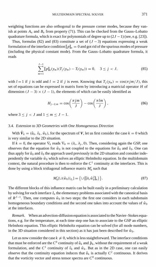
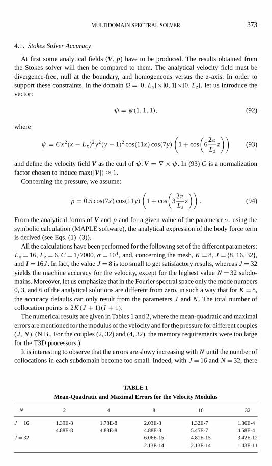
All the calculations have been performed for the following set of the different parameters:Lx = 16, Lz= 6,C= 1/7000, σ = 104, and, concerning the mesh,K = 8, J={8, 16, 32},andI = 16J. In fact, the valueJ= 8 is too small to get satisfactory results, whereasJ= 32yields the machine accuracy for the velocity, except for the highest valueN= 32 subdo-mains. Moreover, let us emphasize that in the Fourier spectral space only the mode numbers0, 3, and 6 of the analytical solutions are different from zero, in such a way that forK = 8,the accuracy defaults can only result from the parametersJ and N. The total number ofcollocation points is 2K (J + 1)(I + 1).

The numerical results are given in Tables 1 and 2, where the mean-quadratic and maximalerrors are mentioned for the modulus of the velocity and for the pressure for different couples(J, N). (N.B., For the couples (2, 32) and (4, 32), the memory requirements were too largefor the T3D processors.)

It is interesting to observe that the errors are slowy increasing withN until the number ofcollocations in each subdomain become too small. Indeed, withJ= 16 andN= 32, there

TABLE 1

Mean-Quadratic and Maximal Errors for the Velocity Modulus

N 2 4 8 16 32

J= 16 1.39E-8 1.78E-8 2.03E-8 1.32E-7 1.36E-44.88E-8 4.88E-8 4.88E-8 5.45E-7 4.58E-4

J= 32 6.06E-15 4.81E-15 3.42E-122.13E-14 2.13E-14 1.43E-11


TABLE 2

Mean-Quadratic and Maximal Errors for the Pressure

N 2 4 8 16 32

J= 16 1.65E-5 2.37E-5 2.82E-5 4.78E-4 0.446.28E-5 6.76E-5 7.71E-5 1.34E-3 0.99

J= 32 1.69E-7 6.01E-6 1.46E-51.94E-7 6.87E-6 1.66E-5

are only nine points along thex axis in each subdomain. For smaller values ofN, the erroris essentially governed by the largest value of thex-space step, which does not depend onthe number of subdomains.

One can also observe in Table 2 that the computation of the pressure is rather accurate andthat the spurious mode-cleaning algorithm proposed in Section 2.2 is efficient. Nevertheless,with J= 16 andN= 32, the results on the pressure are no longer acceptable, whereas theresults for the velocity are still reasonably satisfactory.

Remark1. In some situations, the use of subdomains can improve the accuracy of thenumerical results, especially, when a stiff gradient occurs between two subdomains or if asubdomain is affected to the approximation of a boundary layer [24]. Consequently, it canbe interesting to match the subdomains with the expected solution.

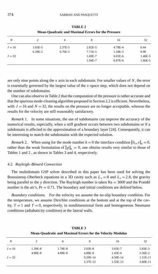
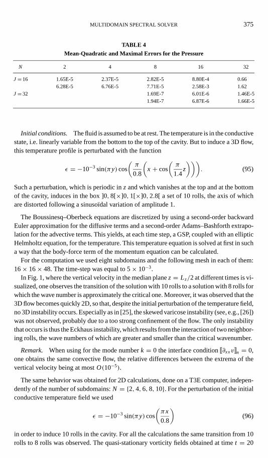
Remark2. When using for the mode numberk= 0 the interface conditionv∂xxvbn= 0,rather than the weak formulation ofvpbn = 0, one obtains results very similar to those ofTables 1 and 2 , as shown in Tables 3 and 4, respectively.

4.2. Rayleigh–Benard Convection

The multidomain GSP solver described in this paper has been used for solving theBoussinesq–Oberbeck equations in a 3D cavity such asLx = 8 andLz= 2.8, the gravitybeing parallel to they direction. The Rayleigh number is taken Ra= 3000 and the Prandtlnumber is the air’s, Pr= 0.71. The boundary and initial conditions are defined below.

Boundary conditions. For the velocity we assume the no-slip boundary condition. Forthe temperature, we assume Dirichlet conditions at the bottom and at the top of the cav-ity, T = 1 andT = 0, respectively, in nondimensional form and homogeneous Neumannconditions (adiabaticity condition) at the lateral walls.

TABLE 3

Mean-Quadratic and Maximal Errors for the Velocity Modulus

N 2 4 8 16 32

J= 16 1.39E-8 1.78E-8 2.03E-8 3.65E-7 5.83E-34.88E-8 4.88E-8 4.88E-8 1.43E-6 3.56E-2

J= 32 9.20E-14 4.50E-14 1.51E-112.37E-13 1.55E-13 3.60E-11


TABLE 4

Mean-Quadratic and Maximal Errors for the Pressure

N 2 4 8 16 32

J= 16 1.65E-5 2.37E-5 2.82E-5 8.80E-4 0.666.28E-5 6.76E-5 7.71E-5 2.58E-3 1.62

J= 32 1.69E-7 6.01E-6 1.46E-51.94E-7 6.87E-6 1.66E-5

Initial conditions. The fluid is assumed to be at rest. The temperature is in the conductivestate, i.e. linearly variable from the bottom to the top of the cavity. But to induce a 3D flow,this temperature profile is perturbated with the function

ε = −10−3 sin(πy) cos

(π

0.8

(x + cos

(π

1.4z

))). (95)

Such a perturbation, which is periodic inz and which vanishes at the top and at the bottomof the cavity, induces in the box ]0, 8[×]0, 1[×]0, 2.8[ a set of 10 rolls, the axis of whichare distorted following a sinuso¨ıdal variation of amplitude 1.

The Boussinesq–Oberbeck equations are discretized by using a second-order backwardEuler approximation for the diffusive terms and a second-order Adams–Bashforth extrapo-lation for the advective terms. This yields, at each time step, a GSP, coupled with an ellipticHelmholtz equation, for the temperature. This temperature equation is solved at first in sucha way that the body-force term of the momentum equation can be calculated.

For the computation we used eight subdomains and the following mesh in each of them:16× 16× 48. The time-step was equal to 5× 10−3.

In Fig. 1, where the vertical velocity in the median planez= Lz/2 at different times is vi-sualized, one observes the transition of the solution with 10 rolls to a solution with 8 rolls forwhich the wave number is approximately the critical one. Moreover, it was observed that the3D flow becomes quickly 2D, so that, despite the initial perturbation of the temperature field,no 3D instability occurs. Especially as in [25], the skewed varicose instability (see, e.g., [26])was not observed, probably due to a too strong confinement of the flow. The only instabilitythat occurs is thus the Eckhaus instability, which results from the interaction of two neighbor-ing rolls, the wave numbers of which are greater and smaller than the critical wavenumber.

Remark. When using for the mode numberk = 0 the interface conditionv∂xxvbn = 0,one obtains the same convective flow, the relative differences between the extrema of thevertical velocity being at mostO(10−5).

The same behavior was obtained for 2D calculations, done on a T3E computer, indepen-dently of the number of subdomains:N = {2, 4, 6, 8, 10}. For the perturbation of the initialconductive temperature field we used

ε = −10−3 sin(πy) cos

(πx

0.8

)(96)

in order to induce 10 rolls in the cavity. For all the calculations the same transition from 10rolls to 8 rolls was observed. The quasi-stationary vorticity fields obtained at timet = 20


FIG. 1. Vertical velocity at timest = 1.2, t = 1.6, t = 2, andt = 2.4 (nondimensional values associatedwith the thermal diffusivity).

for the two extrema of the subdomain number are shown in Fig. 2. For all the consideredvalues ofN, the patterns are identical and the relative differences between the extrema of thevorticity areO(10−6), after spectral interpolations on a unique regular grid. Moreover, thetransition from 10 to 8 rolls agrees with the selection law obtained in [25], which indicatesthat for the present study the only stable patterns should show 7, 8, or 9 rolls.

FIG. 2. Vorticity at timet = 20, computed withN = 2 andN = 10 subdomains.


FIG. 3. Stream-function at timet = 20, for the three stable patterns.

It was interesting to check if the patterns with 7 and 9 rolls would be obtained withour multidomain solver. By changing the perturbation of the initial temperature field, thesepatterns have effectively been obtained. In order to get the 9 (or 7) roll configuration, wesimply induced such flows by substituting in Eq. (96) the mean width of a roll to the 0.8value. In Fig. 3 are shown the quasi-stationary stream-function, obtained at timet = 20 , forthe three stable configurations. When one iduces the 6 roll configuration, then one observesa transition yielding 8 rolls. Thus, for symetry reasons, the 6 and 10 roll configurationsfinally yield, with a gain or a loss of two rolls, exactly the same convective flow. For thesecalculations we usedN = 8 subdomains.

Remark. In order to have an idea of the CPU time with respect to the number of subdo-mains, we give in Table 5 the CPU time needed by the most consuming processor for thepreliminary calculations and for the simulation on the base of 1000 time steps. These resultsare not really favorable, since the total CPU time, i.e. when taking into account the numberof processors, is nearly the same asN ≥ 4 and even begins to increase forN= 10. Suchpoor results were expected for the test-case considered, which does not require many collo-cation points in each subdomain. In this situation, the CPU time needed by the computationof the interface velocity values, with exchanges of data between the different processors,

TABLE 5

CPU Time/Processor for the Preliminary Calculations and for 1000 Simulation Time Steps

N 2 4 6 8 10

Prel. 18.57 3.68 1.66 1.00 0.82Sim. 62.86 22.26 14.46 10.66 9.34


is relatively important. This is no-more true when fine meshes are required, i.e. when themultidomain approach is fully justified.

5. CONCLUSION

We have presented a multidomain procedure for solving in 3D cartesian geometries ofhigh aspect ratio with one homogeneous direction, the generalized Stokes problem (GSP)which results from the finite difference approximation of the incompressible Navier–Stokesequations. The main property of this Fourier–Chebychev spectral solver is that the discreteformulation of the GSP is exactly solved in such a way that the resulting velocity field isperfectly divergence-free. This is obtained in the following manner:

(i) in each subdomain, extended influence matrices are used to compute the boundaryvalues of the pressure when taking into account that the equations are only enforced at theinternal collocation points,

(ii) the velocity components at the interfaces of the different subdomains are computedby using block tridiagonal influence matrices, set up by using appropriate bases in order toenforce the compatibility conditions resulting from the incompressibility constraint.

Moreover, the problem of the spurious modes of pressure has been revisited and a newmethod has been proposed to recover the pressure field.

The computer code has been parallelized for a T3D (T3E) supercomputer and test re-sults have been produced to outline that no drastic loss of accuracy occurs when thenumber of subdomains is increased as soon as the number of collocation points in eachsubdomain is sufficiently high. Finally, the capability of the code has been pointed outby solving a 3D Rayleigh–Bénard problem showing an Eckhaus instability and 2D nu-merical experiments have been achieved to demonstrate the credibility of the numericalresults.

ACKNOWLEDGMENT

All the calculations have been performed on the CRAY T3D (T3E) computer of the IDRIS National Compu-tational Center (91403 Orsay, France). Moreover, we thank J. M. Lacroix for his helpful technical support.

REFERENCES

1. H. C. Ku, R. S. Hirsh, and T. D. Taylor, A pseudospectral method for solution of the three-dimensionalincompressible navier-stokes equations,J. Comput. Phys.70, 439 (1987).

2. G. E. Karnadiakis, M. Israeli, and S. A. Orszag, High order splitting methods for the incompressible navier-stokes equations.J. Comput. Phys.97, 415 (1991).

3. T. N. Phillips and G. W. Roberts, The treatment of spurious pressure modes in spectral incompressible flowcalculations,J. Comput. Phys.105, 150 (1993).

4. O. Botella, On the solution of the navier-stokes equations using chebyshev projection schemes with thirdorder accuracy in time,Comput. & Fluids116, 107 (1997).

5. A. Batoul, H. Khallouf, and G. Labrosse, Une méthode de résolution directe (pseudo-spectrale) du problèmede stokes 2d/3d instationnaire. application à la cavite entrainee carree.C.R. Acad. Sci. Paris319, (II), 1455(1994).

6. M. Azaiez, A. Fikri, and G. Labrosse, A unique grid spectral solver of the nd cartesian unsteady stokes system,illustrative numerical results.Finite Elements in Analysis and Design16, 247 (1994).


7. P. Haldenwang and A. Garba, Pressure solvers of infinite order for 2d/3d generalized stokes problem, unpub-lished.

8. C. Canuto, M. Y. Hussaini, A. Quarteroni, and T. A. Zang,Spectral Methods in Fluid Dynamics(Springer-Verlag, Berlin, 1988).

9. L. Kleiser and U. Schumann, Treatment of incompressibility and boundary conditions in 3D numerical spectralsimulations of plane channels flows, inProc. 3rd GAMM Conf. Numerical Methods in Fluid Mechanics, Noteson Numerical Fluid Mechanics, Vol. 2 (Vieweg, Braunschweig, 1980), p. 165.

10. L. Tuckerman, Divergence-free velocity field in non periodic geometries,J. Comput. Phys.80, 403 (1989).

11. M. R. Schumack, W. W. Schultz, and J. P. Boyd, Spectral method solution of the stokes equations on non-staggered grids,J. Comput. Phys.94, 31 (1991).

12. G. Danabasoglu, S. Biringen, and C. L. Streett, Application of the spectral multidomain method to the navier-stokes equations,J. Comput. Phys.113, 155 (1994).

13. H. H. Yang and B. Shizgal, Chebyshev pseudospectral multi-domain technique for viscous flow calculation,Comput. Methods Appl. Mech. Engrg.118, 47 (1994).

14. M. Azaiez and A. Quarteroni, A spectral stokes solver in domain decomposition methods,Contemp. Math.180, 151 (1994).

15. W. Couzy and M. O. Deville, A fast schur complement method for the spectral element discretization of theincompressible navier-stokes equations,J. Comput. Phys.116, 135 (1995).

16. A. Quarteroni, Domain decomposition methods for the incompressible Navier–Stokes equations, inECCOMAS’94 Conference, Stuttgart, 1994, edited by S. Wagner, E. H. Hirschel, J. P´eriaux, and R. Piva,p. 72.

17. J. P. Pulicani, A spectral multi-domain method for the solution of 1d helmholtz and stokes type equations,Comput & Fluids16(2), 207 (1988).

18. I. Raspo, J. Ouazzani, and R. Peyret, A direct chebyshev multidomain method for flow computation withapplication to rotating systems,Contemp. Math.180, 533 (1994).

19. I. Raspo, J. Ouazzani, and R. Peyret, A spectral multidomain technique for the computation of the czochralskimelt configuration,Int. J. Num. Meth. Heat Fluid Flow6, 31 (1996).

20. P. Le Qu´ere and T. Alziary de Roquefort, Computation of natural convection in two-dimensional cavities withchebyshev polynomials,J. Comput. Phys.57, 210 (1985).

21. R. K. Madabhushi, S. Balachandar, and S. P. Vanka, A divergence-free chebyshev collocation procedure forincompressible flows with two nonperiodic directions,J. Comput. Phys.105, 199 (1993).

22. S. Balachandar and R. K. Madabhushi, Notes: Spurious modes in spectral collocation methods with twonon-periodic directions,J. Comput. Phys.113, 151 (1994).

23. C. Bernardi and Y. Maday,Approximations Spectrales de Problemes aux Limites Elliptiques(Springer-Verlag,Paris, 1991).

24. R. Peyret, The chebyshev multidomain approach to stiff problems in fluid mechanics,Comput. Meth. Appl.Mech. Eng.81, 129 (1990).

25. J. C. Mitais, P. Haldenwang, and G. Labrosse, Selection of 2D patterns near the threshold of the Rayleigh-Benard convection, inProc. 8th Heat Transfer Int. Conf., edited by C. L. Tien, V. P. Carey, and J. K. Serrell,Vol. 4, Hemisphere publishing corporation (San Francisco, USA, 1986), p. 1545.

26. H. L. Swinney and J. P. Gollub,Hydrodynamics Instabilities and the Transition to Turbulence(Springer,Berlin Heidelberg, New York, 1981).

a divergence-free multidomain spectral solver of …rpas/publis/jcp98.pdfjournal of computational...

Documents