290

A dynamic-economic model for container freight market

Meifeng Luo, Lixian Fan and Liming Liu

Department of Logistics and Maritime Studies, The Hong Kong Polytechnic University, Hong Kong.

Abstract

This paper presents a dynamic-economic model analyzing the fluctuation of container freight rate due to the interactions between the demand for container transportation services and the container fleet capacity. The demand for container transportation services is derived from international trade and is assumed exogenous. The container fleet capacity increases with new orders made two years ago, proportional to the industrial profit. Assume market clears each year, the shipping freight rate will change with relative magnitude of demand and supply shifts.

The dynamic model is estimated using the world container shipping market statistics from 1980 to 2008, applying the three-stage least square method. The estimated parameters of the model have high statistical significance, and the overall explanatory power of the model is above 90%. The short-term in-sample prediction of the model can largely replicate the container shipping market fluctuation in terms of the fleet size dynamics and the freight rate fluctuation in the past 20 years. The prediction of the future market trend reveals that the container freight rate would continue decreasing in the coming three years if the demand for container transportation services grows less than 8%.

Keyword: container freight, economic-dynamic model, Empirical analysis, market forecast

1. Introduction

Within a short history of containerization, transportation of containerized goods by sea has thoroughly harnessed the possibility of trade among nations with different comparative economic advantages. Continued specialization and technological progress have boosted the efficiency in global shipping and port operation in the past two decades, making container transportation the indispensable soil for global trading firms to thrive in the increasingly competitive economic environment. Recent statistics shows that while world seaborne trade has been doubled from 3631 million tons in 1985 to 7852 million tons in 2007, containerized trade has increased almost 8 times within the same period from 160 million tons to 1257 million tons1. This demonstrates the increasing role of container transportation in the world seaborne trade, and its contribution to the global economy.

Regardless of the booming global seaborne trade and containerization, the fluctuated container freight rate, as shown by the container time charter rate in recent two decades ( Figure 1), unhinged the profitability in container shipping industry. The high demand for container shipping services hastened shipping companies to order new container vessels with bigger size and higher efficiency, to attract global customers with better services at lower cost, and to gain larger shares in the global competitive shipping market. Companies with the most up-to-date container vessels can out-perform the others with faster and reliable services at a lower unit cost. While reducing sea transportation cost can induce additional demand, it also agonize the companies with less efficient fleets. The usual practice of ‘passing the rent to shippers’ can decrease the freight rate, dissipate rent, diminish profit at the industry level, and even make some companies bankrupt. According to Drewry Shipping Consultants Ltd., comparing with 2006, global carriers moved 14.7% more cargo, but earned1.2 percent less revenue in 2008. On the main east-west trade routes, aggregated losses of the carriers amounted to

1 Data source: Shipping Review and Outlook 2008

291

$2.4 billion, an 8% net loss. Maersk Line, the world largest shipping line with more than 16% of the world’s liner fleet, has suffered a $568 million loss in 2006.

Figure 1: Container time charter rate index 1993-2008 Containership Timecharter Rate Index (1993-2008)

40

60

80

100

120

140

160

180

93 94 95 96 97 98 99 00 01 02 03 04 05 06 07 08

$/TEU 1993=100

The low freight rate in shipping cycle not only has significant negative impact on business operations and investment decision, but also brought extensive concerns at both national and international level. Bankers, who financed the building or purchasing of ships, bear high financial risks due to the insolvency of the ship-owners at low freight rate. According to Volk (1984), most of the ship investment activities are concurrent to the high freight rate. Goulielmos and Psifia (2006) point out that bankers financed 75-80% of the ship construction cost. Therefore, it is very important for the bankers to understand the shipping cycle and take it into consideration in making loan decisions.

Low freight rate and thin profit in shipping industry can create extensive concerns in maritime policy and administration. ‘Safer Shipping and Cleaner Ocean’, once was a mission statement for the International Maritime Organization, resonates the wide concerns over the substandard vessels and crews, two critical factors for maritime accidents that caused the loss of lives and properties at sea, as well as marine environmental pollution. These undesirable incidents most likely follow when ship-owners have insufficient earnings to keep regular maintenances and continued trainings for the crew. To stay in business when the freight rate is low, ship operators have to reduce operation cost in vessel maintenance and manning, even replacing the qualified crew with inexperienced, low salary ones. This can multiply substandard vessels, impair maritime safety, heighten maritime casualty, and undermine sustainability in maritime shipping. According to a report prepared by SSY Consultancy and Research Ltd. for OECD Maritime Transportation Committee, low freight rate in the past 30 years is the most important factor in substandard shipping, which has caused huge economic losses.

From the perspective of national and regional public policy, perhaps the major concern is the mass layoff from shipping industry at low freight rate. When the freight revenue cannot cover its operating cost, a shipping company has to layup a ship and layoff its employees. This is particularly harmful to those developing countries supplying a large maritime work force or providing various kinds of services to the shipping industry. The massive layoffs from shipping industry facing low freight rate can significantly increase the unemployment rate in these countries. In January 9, 2008, having suffered huge losses in 2006 and very low profit in 2007, Maersk Line announced in Los Angeles Times that it plans to layoff as many as 3,000 people from 25,000 employees in its container division. On November 6, 2008, as part of the global layoff plan, Maersk A/S announced that it will cut 700 positions in the Chinese market by 2009, and shut down the global services center in Guangzhou. This province has already suffered massive layoffs recently from the shutting down of many manufacturers facing the weak exporting demand. Further layoff from the shipping company would further exacerbate the economic situation in this region.

The importance of shipping cycle in both private business operation and public sectors has, unsurprisingly, motivated numerous efforts to understand, describe, model, and predict the fluctuation

292

of shipping freight rate. Martin Stopford (2009), for example, described the shipping cycle in the past 266 years, discussed its characteristics, frequency, and difficulties in prediction. Freight market analysis is the first area for applied econometrics. Tinbergen and Koopmans, two well-known pioneers in the econometrics, actually started their econometric analysis in shipping (Beenstock and Vergottis, 1993). Tinbergen investigated the sensitivity of freight rates to changes in demand and supply. Koopmans proposed the first theory to forecast tanker freight rates, assuming market equilibrium between demand and supply. He explained the dynamic behavior of the tanker market by investigate the interrelationship between the market size, freight rate, and shipyard’s activity. Since then, many different models have been developed for the tanker and bulk carrier market analysis. Beenstock and Vergottis (1993) developed a market equilibrium model assuming explicitly profit optimization in supply side, and perfect competition on the demand. They tested the model for tanker and dry bulk shipping market using annual data. This work is recognized as a milestone in econometric analysis of shipping market that “heavily influenced” the modern analysis of bulk shipping markets (Glen, 2006). The most recent work that follows BV’s model is Tvedt (2003), who combined structural and econometric stochastic methods, and built a continuous stochastic partial equilibrium model for the freight and new building market. He found that the equilibrium freight rate process is close to that of a standard geometric mean reversion process.

Despite the significant contribution of container shipping in world seaborne trade, literature on economic modeling and statistical analysis of the container shipping market is scarce. This paper fills the gap by building a dynamic-economic model for container shipping market and testing it using annual data in recent 28 years. Furthermore, without assuming individual behavior in ship investment and operation, this paper reveals the significance of collective market adjustment principles using the observed data, without involving complexities in individual behavior analysis, such as market competition strategies, speculation, and hedging.

This paper lay out as follows. It first describes the theoretic model on the container shipping freight rate and container fleet dynamics. Then, it explains the econometric process for estimating the structural model, the data, the regression results, as well as the stability test of the model. After that, the paper presents an in-sample model prediction to compare with the actual freight data in the study period, and a validity test by calculating the forecast errors for 2007 and 2008 using different estimated models. As an application, it presents the model predictions for future container shipping market between 2009-2013, under different assumptions on the increasing rate of future container shipping demand, and possible cancellation on the new orders. The purpose of this prediction is to alert the decision makers on the possible risks and short-term market trends in container shipping sector. The last section is summary and conclusion.

2. Theoretical model

As in dry bulk and tanker market, container shipping market also includes second-hand market, new-building market and scraping market. Several assumptions are made to simplify the model and focus on the freight market.

First, as container shipping industry is relatively new and the life time of a container vessel is usually more than 30 years, the scraping activity only starts recently and the size of the scraping is just a small fraction of the total fleet size. The average proportion of demolition to world container fleet capacity is only 0.593% from 1994 to 2007. Thus we can ignore the impact of scraping on container fleet capacity.

Secondly, we assume that the second hand market will not affect the container freight market. As trade in the second hand market does not change the usage of a container vessel, it does not affect the world container fleet capacity.

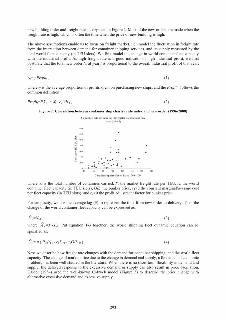
To further simplify the model, we assume new building market will not affect the container freight market. When a shipping company considers placing a new order, the main decision variable is the freight rate, not the new building price. Statistics show that there is a high positive correlation between

293

new building order and freight rate, as depicted in Figure 2. Most of the new orders are made when the freight rate is high, which is often the time when the price of new building is high.

The above assumptions enable us to focus on freight market, i.e., model the fluctuation in freight rate from the interaction between demand for container shipping services, and its supply measured by the total world fleet capacity (in TEU slots). We first model the change in world container fleet capacitywith the industrial profit. As high freight rate is a good indicator of high industrial profit, we first postulate that the total new order Nt at year t is proportional to the overall industrial profit of that year,i.e.,

Nt= ·Profitt , (1)

where is the average proportion of profits spent on purchasing new ships, and the Profitt follows thecommon definition:

Profitt=PtYt - c1Xt - c2OILt , (2)

Figure 2: Correlation between container ship charter rate index and new order (1996-2008)

Correlation between container ship charter rate index and neworder (r=0.48)

0

200

400

600

800

1000

1200

1400

40 60 80 100 120 140 160 180

Container ship time charter Index 1993=100

New

orde

r (K

TEU

slot

s)

where Yt is the total number of containers carried, Pt the market freight rate per TEU, Xt the worldcontainer fleet capacity (in TEU slots), OILt the bunker price, c1>0 the constant marginal/average costper fleet capacity (in TEU slots), and c2>0 the profit adjustment factor for bunker price.

For simplicity, we use the average lag ( ) to represent the time from new order to delivery. Then thechange of the world container fleet capacity can be expressed as:

tX =Nt- , (3)

where =Xt-Xt-1. Put equation 1-3 together, the world shipping fleet dynamic equation can be specified as:

tX

tX = ·( Pt- Yt- - c1Xt- - c2OILt- ) . (4)

Next we describe how freight rate changes with the demand for container shipping, and the world fleetcapacity. The change of market price due to the change in demand and supply, a fundamental economicproblem, has been well studied in the literature. When there is no short-term flexibility in demand and supply, the delayed response to the excessive demand or supply can also result in price oscillation. Kaldor (1934) used the well-known Cobweb model (Figure 3) to describe the price change withalternative excessive demand and excessive supply.

294

Figure 3: The cobweb model

Q1 Q2Q3

P1

P3

P2

Supply

Demand

Quantity

Price

Q1 Q2Q3

P1

P3

P2

Supply

Demand

Quantity

Price

When the market price is high at time 1, the quantity demand (Q1) at P1 is lower than the quantitysupplied (Q2). The excessive supply (Q2-Q1) will reduce the price down to P2 in the next period. At thisprice level, the quantity demanded (Q2) is higher than the quantity supplied (Q3). This excessivedemand (Q2-Q3) will increase the price. The stability of the market price in the long run will depend on the relative price sensitivity in demand and supply. According to this theory, the change of market price can be written as:

)( ttt XYP , (5)

where =Pt-Pt-1, the price change in year t, and the reuse rate of a TEU slot. This equation states thatprice will increase when there is excessive demand, and drops with excessive supply.

tP

Consider the nature of maritime transportation for the containerized goods. First, shipping freight rate is flexible and negotiable between the shipper and carrier. Second, it is well-known that the marginal cost for additional container, especially in liner services, is very low. Container carriers can always acceptone more box as long as it covers the marginal cost. Third, there are many ways to provide short-termshipping services facing sudden demand increase, including increase loading factors and increase cruise speed. Demand and supply are both flexible enough in container shipping industry, especially on annuallevel. This conforms to BV’s model assumption in market equilibrium in his econometric analysis fordry bulk and tanker market (Beenstock and Vergottis, 1993).

Assume market clears each year, market freight rate changes with exogenous demand shift caused bythe exogenous change in international trade, and the supply shift as more container vessels add to theworld container fleet capacity. From the demand side, with the increase in international trade, thedemand for container shipping will increase even when the market freight rate is constant. On the supply side, when more capacity is added to the industry, more container ships are available in the market to provide more services even with the same market price. An illustration of how market price changes with relative shifts in demand and supply are given in Figure 4.

295

Figure 4: Illustrated price dynamics with demand and supply shift

Qt Qt+1

Pt

Supply

Demand

Quantity

Price

P’t+1

P’’t+1

Dt

Dt+1

St St+1

S’t+1

S’’t+1

Qt Qt+1

Pt

Supply

Demand

Quantity

Price

P’t+1

P’’t+1

Dt

Dt+1

St St+1

S’t+1

S’’t+1

Assuming at time t, the market clearing price and quantity, the intersection of demand Dt and supply St,are (Pt, Qt). If there are equal amount of supply and demand shifts (Dt Dt+1, St St+1), The new marketclearing price will remain unchanged, while the quantity will be Qt+1. This confirms to the description by Tvedt (2003). If the supply only shift to , less than the demand shift, the market clearing price

will increase to . On the other hand, if the supply shift to , more than demand shift, the market

clearing price will be drop to . Applying this to the container market freight rate with respect to thesupply and demand change, we postulate:

'1tS

'1tP "

1tS"

1tP

)( ttt XYP , (6)

where Yt and Xt are the changes in the total number of containers handled and the fleet capacity,respectively, >0 is a constant representing average annual container slot reuse rate, and >0 is theprice adjustment factor due to the demand and supply shifts.

Equation (4) and (6) are the two dynamic equations that describe the two major forces in container shipping market. The interaction of these two forces can be illustrated in Figure 5. Assume that marketdemand for container shipping increases exogenously. When the price is high (at A in Figure 5), the high industry profit will bring up the number of new orders (denoted by larger upper triangles). If the delivery of new containers ships resulted in a larger increase in capacity than that in demand, the market price will fall. When this happens (at B), there will be very few new orders (denoted by smaller upper triangle) by the speculators, but the ships ordered in the previous two or three years when the freight rate is increasing will keep adding to the existing fleet, which will accelerate the decreasing rate of freight rate. This downward trend in the market freight rate will end when the capacity increase slower than thedemand increase (at point C where the delivery is very small). Because of the few new orders during theprevious three or four years, the low supply in shipping capacity will push up the market price. When the market price is increasing, there will be a stronger incentive to order more new container vesselsagain, which will lead to a new shipping cycle.

296

Figure 5: Illustration of shipping market dynamics

Frei

ght r

ate

Capacity

AB

C

New orderDelivery

To test the theory, using the annual data for container market freight rate, the total number of containers handled, the world fleet capacity in TEU slots, and bulker price from 1980 to 2006, we estimated the parameters in the statistical model using the above data, which will be explained in next section.

3. Quantitative analysis of the dynamic model

We construct the statistical model by transfer the equation (4) and (6) into linear forms as follows:

ΔXt = Pt- Yt- - c1Xt- - c2OILt- + 1t= 1Pt- Yt- – 2Xt- – 3OILt- + 1t , (7) ΔPt= ΔYt - ϕΔXt+ 2t= 4ΔYt – 5ΔXt+ 2t . (8)

The last term it in each equation is the error term. Although Yt- appears in the first equation and Ytappears in the second, they are not contemporaneously correlated. The first equation can be estimated by itself. As ΔXt appears on the left-hand side of the first equation and the right-hand side of the second equation, the error terms are not independent (cov(ΔXt, 2t)= 12). Thus we apply Simultaneous Equation (SE) method to estimate the coefficients in the system. The first step in SE is to rewrite equation (7) and (8) into reduced form by substituting Xt into the second equation:

ΔXt = 1Pt- Yt- – 2Xt- – 3OILt- + 1t

ΔPt= 4ΔYt – 5 1Pt- Yt- + 5 2Xt- + 5 3OILt- + 5 1t + 2t = 4ΔYt – 5Pt- Yt- + 6Xt- + 7OILt- + 8 1t + 2t

As can be seen from the reduced form, the two equations are not independent. Thus, two stage least square (2SLS) is not sufficient to make full use of the correlation between error terms. Therefore, 3SLS method was applied in the estimation process for the coefficients in the reduced form. The estimated parameters are transferred back to the structural equation. The instrument variables used in 3SLS include all the exogenous variables and predetermined variables. The estimation process follows the standard treatment as specified in Judge et al (1988), so it will not be included in this paper.

3.1. Data

Demand for container transportation services is derived demand from global trade, which is determined by the comparative advantage of individual countries. We take demand as given to avoid modeling the global trade. Besides, as unsatisfied demands are not observable, the assumption on market clearance each year enables us to use the container throughput as quantity demanded. The data used in this study and their sources are included in

297

Table 1.

The world container throughput, from the Drewry Annual Container Market Review and Forecast, is the total port throughput, including the empties and transshipment. We use container throughput, not the world trade volume, as the demand for container shipping services, for the following two reasons. First, the world trade volume includes many commodities that are not carried by ships. Further, not all the seaborne trade is containerized. The containerization rate is changing. To convert world trade volume of different commodities to number of TEUs is not currently feasible. Secondly, container throughputs are a more appropriate data to use. Although there are empties, transshipments and possible double counting, they are actually part of the demand for container transportation services. Thus, we used container throughput, rather than the world trade volume, as the demand for container transportation services.

The same report from Drewry also provides the container freight rate, which is the weighted average of Transpacific, Europe-Far East and Transatlantic trades, inclusive of THCs (Terminal Handing Charge) and intermodal rates. This variable is a synthetic index, representing the average level of container freight rate. This can be an index for shipowners’ unit revenue. As Drewry only reported freight rates from 1994-2006, we have to calculate the missing part (1980-1993) from General Freight Index in Shipping Statistics Yearbook 2007, using a simple statistical equation between container freight rate and the general freight index during 1994 and 2006. The container fleet capacity data are also from the Drewry Annual Container Market Review and Forecast.

On the supply side, we use the data from Clarkson Research Services Limited 2008, which include the new order, delivery, and scrap data in TEU slots and bunker prices. Although some of these data are not used in estimate the main model, they are used in determine whether to include the scrapping market and the shipbuilding lag. Therefore, they are also included in the table.

298

Table 1: Data used in this study and sources

Year Container Throughput

(Yt; K TEU)*

Freightrate(Pt;

$/TEU)*

FleetCapacity (Xt; K TEU)*

Bunker Price(OILt; $/ton)%

Delivery (Nt; K TEU) %

Scrap (St; K TEU) %

New Order (Ot; K TEU) %

1980 38,821 1,762 665.0 307.0 115.8 1981 41,900 1,644 702.0 288.3 38.3 1982 43,800 1,449 745.0 284.8 72.6 1983 47,600 1,441 799.0 243.7 100.6 1984 54,600 1,451 883.0 229.6 130.3 1985 56,170 1,420 1012.0 222.8 131.1 1986 62,200 1,355 1189.0 142.1 140.1 1987 68,300 1,455 1276.3 144.1 92.7 1988 75,500 1,630 1384.7 124.7 116.4 1989 82,100 1,632 1487.9 144.1 102.3 1990 88,049 1,544 1613.2 191.2 133.6 1991 95,910 1,544 1756.0 170.8 152.1 1992 105,060 1,471 1916.3 161.9 167.6 1993 114,920 1,480 2101.3 150.5 200.1 115.9 1994 129,380 1,466 2370.7 133.2 268.8 2.8 472.5 1995 144,045 1,519 2684.0 140.6 330.1 10.9 597.4 1996 156,168 1,434 3048.1 175.1 408.1 21.5 501.5 1997 175,763 1,282 3553.0 157.2 523.1 25.0 203.6 1998 190,258 1,267 4031.5 112.2 529.6 87.3 414.5 1999 210,072 1,385 4335.2 133.0 257.1 51.7 555.2 2000 236,173 1,421 4799.1 231.6 449.1 15.5 956.9 2001 248,143 1,269 5311.0 192.4 623.2 36.1 519.1 2002 277,262 1,155 5968.2 188.2 642.8 66.5 414.2 2003 316,814 1,351 6528.6 230.4 560.7 25.7 2057.0 2004 362,161 1,453 7162.8 313.4 643.0 4.0 1652.9 2005 397,895 1,491 8117.0 458.4 941.5 0.3 1644.3 2006 441,231 1,391 9472.0 524.1 1366.6 20.4 1784.6 2007 496,625 1,435 10805.0 571.3 1321.1 23.8 3060.1 2008 540,611 1,375 12126.0 850.7

Freight rates (Italic part) computed from general freight index (from shipping statistics yearbook) Source: * The Drewry Annual Container Market Review and Forecast 2000-2008

% Clarkson Research Services Limited 2008

3.2. Specification of

As a key factor in shipping market analysis, the shipbuilding lag is ubiquitous in almost all the econometric analysis in this field. Binkley and Bessler (1983) found that shipbuilding construction lag, ranging from eight months to around two years, is one of the most important market features in the bulk shipping market analysis. In our study, we assume constant construction lag during the study period. Further, as we are using annual data, we require the lag to be rounded to an integer. Therefore, we constructed 6 statistical equations between the delivery and the new order data, and selected the most significant one to use in our model.

The regress results of the 6 equations are listed in Table 2. The 2-year lag and 3-year lag are all significant in model 1-6, but R2 in model 5 is much bigger than that in model 6, so we choose =2. This means on average it takes two years to build a container vessel, although bigger ships may take longer and smaller ones may only need several months.

299

Table 2: Modeling of construction lags (p-value in parenthesis) Variable Model 1 Model 2 Model 3 Model 4 Model 5 Model 6 b0 255.5099

(0.0436) 257.6291 (0.0174)

175.4902 (0.0061)

218.035 (0.0035)

297.841 (0.0022)

356.7358 (0.004)

ordert -0.00475 (0.9475)

ordert-1 0.167043 (0.0596)

0.166467 (0.0327)

0.112564 (0.0444)

ordert-2 0.211811 (0.0361)

0.210334 (0.0152)

0.251027 (0.0021)

0.313896 (0.0007)

0.434595 (0.0003)

ordert-3 0.27146 (0.0156)

0.26916 (0.0037)

0.267692 (0.0013)

0.279653 (0.0028)

0.441905 (0.0043)

ordert-4 -0.20405 (0.3479)

-0.212 (0.1867)

R-squared 0.966885 0.966844 0.954026 0.914724 0.745311 0.615101

3.3. 3SLS results of the system parameter

The regression result from the 3SLS process for the structure equation, including the estimates of the structural parameters and their corresponding t-values, R2 and adjust R2 are listed below:

Xt= 0.0000034Pt-2Yt-2 – 0.06411Xt-2 – 0.438215OILt-2 (5.00) (-1.52) (-2.72) t-value

R2=0.95, Adjusted R2=0.947

Pt=0.00894 Yt – 0.378085 Xt (3.96) (-4.01) t-value

R2=0.353, Adjusted R2=0.328

All the estimated coefficients (a1 through a5 in equation 7 and 8) are significant at least at 90% confidence level, and the coefficient estimates on revenue (a1), bunker (a3), demand (a4) and supply (a5)are all significant at 99% confidence level.

To evaluate the overall explanatory power of the whole system, we use the error sum of squares (SSE) and total variance (SST) in respective regression equation to construct the overall coefficient of determination for the system. From first equation, we have SSE1=200197, SST1=4125572. From the second equation, we get SSE2=158424, and SST2=245222. So the overall R2 could be written as:

21

212 1SSTSSTSSESSER

++−= =0.9179

which indicates the over explanatory power of the system is about 92%.

3.4. Explanation of the regression results

To understand the regulation results, we first transform them into the dynamic equations in equation (4) and (6):

Xt =0.0000034Pt-2Yt-2 – 0.06411Xt-2 – 0.438215OILt-2 =0.0000034(Pt-1Yt-2 – 19080Xt-2 – 130421OILt-2 ) (9)

Pt = 0.00894 Yt – 0.378085 Xt = 0.00894( Yt -42.27 Xt ) (10)

300

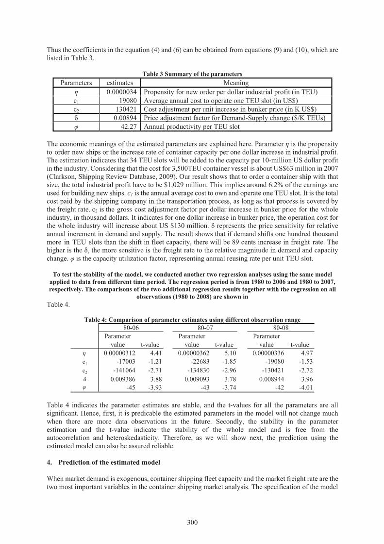
Thus the coefficients in the equation (4) and (6) can be obtained from equations (9) and (10), which are listed in Table 3.

Table 3 Summary of the parameters Parameters estimates Meaning

0.0000034 Propensity for new order per dollar industrial profit (in TEU) c1 19080 Average annual cost to operate one TEU slot (in US$) c2 130421 Cost adjustment per unit increase in bunker price (in K US$)

0.00894 Price adjustment factor for Demand-Supply change ($/K TEUs) 42.27 Annual productivity per TEU slot

The economic meanings of the estimated parameters are explained here. Parameter is the propensity to order new ships or the increase rate of container capacity per one dollar increase in industrial profit. The estimation indicates that 34 TEU slots will be added to the capacity per 10-million US dollar profit in the industry. Considering that the cost for 3,500TEU container vessel is about US$63 million in 2007 (Clarkson, Shipping Review Database, 2009). Our result shows that to order a container ship with that size, the total industrial profit have to be $1,029 million. This implies around 6.2% of the earnings are used for building new ships. c1 is the annual average cost to own and operate one TEU slot. It is the total cost paid by the shipping company in the transportation process, as long as that process is covered by the freight rate. c2 is the gross cost adjustment factor per dollar increase in bunker price for the whole industry, in thousand dollars. It indicates for one dollar increase in bunker price, the operation cost for the whole industry will increase about US $130 million. represents the price sensitivity for relative annual increment in demand and supply. The result shows that if demand shifts one hundred thousand more in TEU slots than the shift in fleet capacity, there will be 89 cents increase in freight rate. The higher is the , the more sensitive is the freight rate to the relative magnitude in demand and capacity change. is the capacity utilization factor, representing annual reusing rate per unit TEU slot.

To test the stability of the model, we conducted another two regression analyses using the same model applied to data from different time period. The regression period is from 1980 to 2006 and 1980 to 2007, respectively. The comparisons of the two additional regression results together with the regression on all

observations (1980 to 2008) are shown in Table 4.

Table 4: Comparison of parameter estimates using different observation range

Parameter value t-value

Parameter value t-value

Parameter value t-value

0.00000312 4.41 0.00000362 5.10 0.00000336 4.97c1 -17003 -1.21 -22683 -1.85 -19080 -1.53c2 -141064 -2.71 -134830 -2.96 -130421 -2.72

0.009386 3.88 0.009093 3.78 0.008944 3.96-45 -3.93 -43 -3.74 -42 -4.01

80-06 80-07 80-08

Table 4 indicates the parameter estimates are stable, and the t-values for all the parameters are all significant. Hence, first, it is predicable the estimated parameters in the model will not change much when there are more data observations in the future. Secondly, the stability in the parameter estimation and the t-value indicate the stability of the whole model and is free from the autocorrelation and heteroskedasticity. Therefore, as we will show next, the prediction using the estimated model can also be assured reliable.

4. Prediction of the estimated model

When market demand is exogenous, container shipping fleet capacity and the market freight rate are the two most important variables in the container shipping market analysis. The specification of the model

301

enables us to predict the fleet capacity increases in two years based on the current container throughput, freight rate, and bunker price. The relative capacity increase, determined endogenously from the first dynamic equation, can then be used to predict the adjustment in freight rate, for given container transportation demand.

4.1. In-sample prediction

To demonstrate the explanatory power of our model, we first compare the model prediction with the actual date. An in-sample prediction for the market fleet capacity and the freight rate, together with the actual freight rate and fleet capacity from 1980 to 2008 (called 80-08 model), are provided in Figure 6.

Figure 6: In-sample prediction of fleet capacity and freight rate (1980-2008)

08

96

98

00

02

04

06 07

1,000

1,100

1,200

1,300

1,400

1,500

1,600

1,700

1,800

0 2,000 4,000 6,000 8,000 10,000 12,000 14,000

Fleet Capacity (thousand TEU slots)

Frei

ght R

ate

($ p

er T

EU)

Actual Predict

Figure 6 exhibits that the fleet capacity increases faster in recent years than that of the earlier years, as the horizontal distances between each pair of dots are wider in recent years. The freight rate is generally decreasing over time, and it is oscillating around the US$1,400 in recent years. Our prediction can largely replicate the trend of the actual freight rate change. The predicted fleet capacity each year is very close to the real fleet capacity (They are basically in the same vertical line). The predicted fleet capacity and the freight rate for 2008 (12,030 thousand TEU slots, US$1,329 per TEU) are very close to the real capacity and freight rate (12,126 thousand TEU slots, US$1,375 per TEU).

To check the stability of model prediction, we estimated the model using the observation from 1980 to 2006 to predicate the freight rate and fleet capacity for 2007 and 2008. The actual value of fleet capacity and freight rate, and the predicated ones with 80-06 model and 80-08 model are shown in Table 5.

Table 5: Comparison of predicted values using different model results

Year FleetCapacity

FreightRate

FleetCapacity(error)

FreightRate(error)

FleetCapacity(error)

FreightRate(error)

10691 $1,399 10744 $1,3821.06% 2.52% 0.56% 3.66%

11873 $1,318 12030 $1,3292.09% 4.14% 0.79% 3.36%

2008

80-06 model

10805 $1,435

12126 $1,375

80-08 modelPredicted valueActuall value

2007

Note: Fleet Capacity in thousand TEUs

302

Comparing the predicted results from two different models, it is obvious that both models can predicate fleet capacity in relatively smaller error than the prediction of freight rate. The error margin for freight rate prediction ranges from 2.52% to 4.14%, while prediction for fleet capacity is within 2.10%. In either model, the prediction values are within 5% error margin, which indicate a good fix, even for the out of sample prediction. Therefore, in out-sample prediction for future container market, the 80-08 model prediction result will be presented.

4.2. Prediction for the future container shipping market.

The purpose for this dynamic-economic model is to predict the future market situation, so that the decision makers could anticipate and respond possible market changes. The first necessary step is to assume the future container demand growth rate based on the past information. Our data shows that average increasing rate of the container throughput in the past 27 years from 1981 to 2007 is about 9.94%, with highest 14.31% in 2004, and lowest 2.88% in 1985. Considering the possible range of container transportation demand in the coming years, we assume three different growth rates (5%, 8% and 10%) for the year from 2009 to 2013.

Under the current global financial crisis, the shipping sector not only refrained from ordering new ships, but also motivated to cancel existing orders. According to recent statistics from Lloyd’s register, total new orders in October 2008 have been dropped by 90% comparing with the same period in 2007. According to Clarkson, there are totally 94 new order cancellations. Cancellations can reduce the number of new deliveries to the market and slow down the freight rate decrease. As recent new orders are easier to cancel, we assume 10% cancellation rate for the new orders made in 2007, and 20% cancellation rate for the new orders made in following years. The continued cancellation after 2008 reflects the change in industry behavior for making new orders, a more prudent measure facing the financial crisis. The prediction of the market freight rate and the fleet capacity from year 2009 to 2013 are shown in Figure 7. Actual data for 2007 and 2008 are included in the figure just to show the trend.

Figure 7: Forecast of future container shipping market from 2007 to 2013

201020082007

2013

600

800

1000

1200

1400

1600

1800

8000 10000 12000 14000 16000 18000 20000 22000Fleet Capacity (thousand TEU slots)

Frei

ght R

ate

($ p

er T

EU)

5% growth

5% growth rate, with 10% cancel rate in 2007 and 20% after

8% growth

Drewry predicted growth

8% growth rate, with 10% cancel rate in 2007 and 20% after

10% growth rate

Drewry predicted growth rate (8.6%, 8.7%, 9.1%, 8.9%, 8.7% from 2009 to 2013 respectively)

Figure 7 also includes the market prediction based on Drewry’s forecast on possible growth rate of the future container transportation demand. According to that, our model shows that freight rate will continue decreasing until 2010, then increase slowly until 2013. This reveals the excessive capacity in the world container fleet. Our prediction base on the 10% growth rate is more optimistic than the Drewry, reflecting the best situation for quick recovery. However, high freight rate can encourage larger new orders, causing an earlier decreasing market in 2011. Our prediction using 8% growth rate in future container throughput represents a more conservative prediction than the Drewry’s. The freight

303

rate will be below US$1,200 from 2010 to 2013, and will recover after 2011. In this case, the new order activity will decrease, as the net profit will decrease in the industry. Considering the current financial crisis and the low demand in the container shipping, if the future demand increasing rate was only 5%, then the freight rate will be below US$1,100 in 2009, close to US$800 in 2010, and further below US$800 in 2011.

Cancellations of new orders could slow down the dropping of the freight rate. For 8% future growth rate, if 10% of the new orders made in 2007 and 20% of new orders made afterwards were canceled, the freight rate would stop decreasing in 2010 when it was slightly lower than US$1,200, and it could better than predicated rate based on the Drewry’s prediction later. For 5% growth rate, under the same cancellation scheme, the predicted freight rates were higher than that in no cancellation case, and would never below US$800. This shows that cancellations are beneficial to prevent further drop in freight rate, if the current financial crisis has a serious negative impact on the world economy and international trade. Because of the comparatively higher freight rate, when there is cancelation, the new order would be higher than the case when there is no cancellation; therefore, the capacity with cancellation is larger than the capacity without cancellation.

5. Summary and Conclusion

We presented a dynamic-economic model for container shipping market characterized by the container shipping freight rate and the global container fleet capacity. The model postulates the changing of equilibrium freight rate under demand and supply shifts in the container shipping market. The world container fleet capacity is augmented by the number of new orders which is proportional to the industrial profit earned two years ago. The quantity demanded for container transportation services, as a derived demand from international trade, is assumed to be exogenously determined in the model.

The model parameters were estimated using the global container shipping market data from 1980 to 2008, based on the available data from Drewry and Clarkson. Considering the interdependency of the two dynamic equations, a three-stage least square method was adopted in the regression analysis. The estimated results are quite stable, provided a high goodness of fit, and the parameter estimates are significant above 90% confidence level. The overall model can explain more than 90% of the variations in fleet capacity and freight rate, and the in-sample prediction of the model can largely replicate the actual data within the research period. The errors of in-sample prediction and out-sample prediction for the previous two years, using model estimated using date with different number of observations, reveals that the stability of prediction is within 5% error margin.

As an application of the research, we predicted the future container market from 2009 to 2013, based on different assumptions on the future growth rate in container transportation demand. The result shows that if the world financial crisis were continue to decrease the international trade, the container freight rate could drop to below US$800 in 2011. With decreasing rate of new ordering and the cancellation of existing order, the market freight rate could be saved from reaching such a low level, although the one who cancelled the new order would suffer some immediate losses.

In conclusion, the model can provide information for decision makers in both public policy and private business. The maritime agencies or organization at regional, national and international level can use this information to stabilize the market freight rate, so as to mitigate the negative impact of the recent financial crisis on maritime industry, marine environment, maritime safety, and national, regional and local economy. The bankers can use this information in ship financing decision, to minimize the possible risks caused by the low freight rate. Shipowners and ship operators can also use this method to setup their respective best strategies to prevent or reduce possible losses in the coming several years.

6. Acknowledgements

The work described in this paper was supported by a grant from the Research Grants Council of the Hong Kong Special Administrative Region, China (Project No. B-Q08K).

304

References

Beenstock, M. and Vergottis, A. (1989), An econometric model of the world market for dry cargo freight and shipping. Applied Economics, 21, 339-356. Beenstock, M. and Vergottis, A. (1993), Econometric modeling of world shipping. London.

Binkley, J.K. and Bessler, D. (1983), Expectations in bulk ocean shipping: an application of autoregressive modeling. Review of Economics & Statistics, 65(3), 516-520.

Glen, D.R. (2006), The modeling of dry bulk and tanker markets: a survey. Maritime Policy and Management, 33(5), 431-445.

Goulielmos, A. M. and Psifia, M. (2006), Shipping finance: time to follow a new track?. Maritime Policy and Management, 33(3), 301-320.

Judge, G.G., Hill, R.C., Griffiths, W.E., Lutkepohl, H., and Lee, T.C. (1988), Introduction to the theory and practice of econometrics 2nd ed. John Wiley & Sons.

Kaldor, Nicholas (1934), A Classificatory Note on the Determination of Equilibrium. Review of Economic Studies, vol I (February, 1934), 122-36.

SSY Consultancy and Research Ltd (2001), The cost to users of substandard shipping. Prepared for the OECD maritime transport committee.

Stopford, M. (2009), Maritime economics, 3rd Edition, Routledge, London.

Tvedt, J. (2003), Shipping market models and the specification of freight rate processes. Maritime Economics & Logistics, 5, 327-346.

Volk, B. (1984), Shipping Investment in Recession (Bremen: Institute of Shipping Economics and logistics at Bremen)