a faster algorithm to update betweenness centrality …

Internet Mathematics, 11:403–420, 2015Copyright © Taylor & Francis Group, LLCISSN: 1542-7951 print/1944-9488 onlineDOI: 10.1080/15427951.2014.982311

A FASTER ALGORITHM TO UPDATE BETWEENNESSCENTRALITY AFTER NODE ALTERATION

Rishi Ranjan Singh,1 Keshav Goel,2 S. R. S. Iyengar,1

and Sukrit Gupta3

1Department of Computer Science and Engineering, Indian Institute of Technology,Ropar, Punjab, India2Department of Computer Engineering, National Institute of Technology,Kurukshetra, India3Department of Computer Science and Engineering, PEC University of Technology,Chandigarh, India

Abstract Betweenness centrality is widely used as a centrality measure, with applicationsacross several disciplines. It is a measure that quantifies the importance of a vertex based on thevertex’s occurrence on shortest paths in a graph. This is a global measure, and in order to findthe betweenness centrality of a node, one is supposed to have complete information about thegraph. Most of the algorithms that are used to find betweenness centrality assume the constancyof the graph and are not efficient for dynamic networks. We propose a technique to updatebetweenness centrality of a graph when nodes are added or deleted. Observed experimentally,for real graphs, our algorithm speeds up the calculation of betweenness centrality from 7 to412 times in comparison to the currently best-known techniques.

1. INTRODUCTION

Network centrality measures are used to quantify the intuitive notion of nodes’ importance ina network. There are several application-centric definitions of network centrality measures,the popular ones being degree centrality, closeness centrality, eigenvector centrality, andbetweenness centrality. For background and description of centrality measures, one canrefer to [30, 18, 5].

There are a number of centrality indices based on the shortest path lengths: closenesscentrality [33], graph centrality [14]; and the number of shortest paths: stress centrality[36], betweenness centrality [10, 1] in a graph. Each centrality measure signifies a particu-lar characteristic that a node exhibits. Closeness centrality of a vertex indicates the distanceof a vertex from other vertices. Graph centrality denotes the difference between closenesscentrality of the vertex under consideration and the vertex with the highest closeness cen-trality. Stress centrality simply denotes the total number of shortest paths passing througha vertex.

The idea of betweenness centrality was proposed in [1, 10]. Betweenness centralityof a node v is defined as BC(v) =∑

s �=t �=vεVσst (v)σst

, where σst is the total number of shortest

Addresss corrrespondence to Sudarshan Iyengar, Department of Computer Science and Engineering, IndianInstitute of Technology, Ropar, Nangal Road, Rupnagar Punjab, India – 140001. E-mail: [email protected]

Color versions of one or more of the figures in the article can be found online at www.tandfonline.com/uinm.

403

404 GOEL ET AL.

paths from vertex s to vertex t , and σst (v) is the total number of shortest paths from vertexs to vertex t passing through vertex v.

Betweenness centrality insinuates a more global characteristic, unlike the degreecentrality, which takes into consideration the number of links originating from a node(also called the degree of a node), which is clearly a local characteristic. Betweennesscentrality has found many important applications across different disciplines. It has beenused in the identification of sensitive nodes in biological networks [28]. Betweennessscores an play important role in public transit system networks [34, 8], gas pipeline net-works [7], and waste-water disposal system networks [24]. In protein-protein interaction(PPI) networks, essential proteins can be identified by their high betweenness centrality[19]. This characteristic of proteins can be used to select suitable drug targets [41] forvarious ailments including cancer [16], tuberculosis [35], zoonotic cutaneous leishmani-asis [9], etc. Recently, Nagata et al. [27] proposed a new load-balancing approach thatreduces the blocking probability of request in wavelength-division multiplexing (WDM)networks. In their algorithm, they used betweenness centrality of nodes for adjusting the linkcosts.

Betweenness centrality is also used to identify nodes that are crucial for informa-tion flow in a brain network [17], where different regions of the brain represent nodesin the network and white matter represents the links. With recent advances in Electrical& Electronic Systems (EES systems such as Electronic Control Units used in vehicles)the mechanism of fault isolation and fault detection is of great importance. In [25], itwas observed that the betweenness centrality score of a node is a good basis for rank-ing the fault tolerance monitoring points and that it outperforms the degree centralitymeasure.

Similarly, in supply chain networks [40] it is reported that for a lower level of tolerance(load carrying capacity), more harm is created in the case when a node with high load isdeleted from a network opposed to when a node with high degree is deleted.

[3] An algorithm to calculate betweenness centrality that reduced the time complex-ity from O(|V |3) to O(|V ||E|) for unweighted graphs was suggested in [3]. Since wassuggested in .the real-world networks tend to be large and transient, such algorithms areobservedly impractical if one requires computing the betweenness centrality of nodes ina dynamic network. In [40], experiments were performed to report that the betweennessranking order of vertices before and after being updated in a graph can be significantlydifferent. Most of the real-world networks are dynamic in nature, which calls for designingan algorithm that can update the betweenness centrality of nodes faster than the algorithmsdesigned for static networks. There are several algorithms proposed in [23, 12, 20] to findbetweenness centrality for updating edges in a graph. Most of the currently available litera-ture considers only the case of updating edges, i.e., these algorithms assume that alterationof a node from a graph is equivalent to modifying one or more edges incident on that node.We propose an algorithm that is deg(v)-times faster than the afore mentioned algorithmsin the case of a deletion/addition of a node v.

1.1. Motivation

It is sometimes necessary to calculate betweenness centrality for a network at every stageof transition. With a large network and the current algorithms in use, recalculation becomesdifficult. Some examples of such networks follow.

A FASTER ALGORITHM TO UPDATE BETWEENNESS CENTRALITY 405

Complex communication networks are continuously growing and evolving. Eachnode in a communication network has a maximum capacity for carrying load,1 after whichthe node shuts down and its load is distributed among the remaining nodes. Because ofincreased load, other nodes might shut down and the network might become disconnected.This phenomenon is commonly known as cascading failure. Betweenness centrality of anode corresponds to its load. In scenarios where a node failure is taking place, we need torapidly calculate load of a node and compare it to its load-carrying capacity to determinewhether this node will be able to sustain the extra load that was added to it due to the failureof the previous node. This helps us determine whether a cascading failure will take place.This has applications not only in communication networks but in transport networks and inEES networks, too.

It has been found through experiments conducted [28] that breakdown of nodes withhigher betweenness centrality causes greater harm. In such networks, we can compute asequence of nodes as follows: We start with the given network. At each step, we delete thenode with the highest betweenness centrality, add that node to the sequence and then repeatthis process until the network becomes disconnected. This sequence can be used to decidethe order in which security should be provided to the nodes in the network and to ensure thatif a node in the present network fails, the node with the highest betweenness centrality in theresulting network has enough security and resources. This requires repetitive calculationof betweenness centrality which when done with the conventional algorithm [3], willbe highly inefficient. Similarly, points that have excess load in power grid systems andcomputer networks can be provided with more resources; stations with excess traffic inpublic transit systems can be provided with more measures to redistribute traffic, and sewerlines with higher betweenness centrality can be provided with more frequent maintenanceto prevent blockades. This exercise can also be done after the failure of some random nodein a graph, and appropriate actions on the nodes in the network may be taken thereafter.

Two sequential failure strategies, random and usage based, are being used [25]for fault mitigation analysis. In usage-based failure strategy, it is assumed that usage isproportional to its betweenness centrality. Thus, the node with the highest betweennesscentrality score is most likely to fail in case of usage-based failure strategy. After everyfailure, we need to calculate which node has the highest betweenness centrality and checkif we have reached a preset completion criterion (maybe a threshold value, after whichthe network is so fragmented that it is not usable, or a percentage of nodes) and if itdoes, we can check the number of failures that were required to reach there from the firstfailure. The node with the minimum number of failures required should be monitored morerigorously. This recursive calculation of betweenness centrality is useful in fault mitigationanalysis.

In social networking websites such as Twitter and Facebook, betweenness centralityof a node denotes the number of heterogeneous groups of nodes that the node underconsideration links [37]. Since these nodes are involved in passing information betweenheterogeneous groups of nodes, they are more important than a node with just a higherdegree.2 Also, we may want to determine the next important actor in case the current social

1The amount of information flowing through a node in a communication network is calledits load.

2In the study [15] conducted on the uprising in Egypt, where the social networking site Twitterplayed an important role in the formation of public opinion against Mr. Hosni Mubarak (the thenPresident of Egypt), it was found that these nodes played an important role in shaping public opinion.

406 GOEL ET AL.

network is altered. Such networks are highly dynamic due to the continuous addition andremoval of actors.

In section 2, we present some basic definitions and concepts used in this article.Section 3 contains the algorithm with explanation. Implementation details and results arepresented in Section 4. For synthetic graphs, we tested our algorithm by generating ErdosRenyi graphs with different probabilities. We took both cases of node addition and nodedeletion into consideration and achieved speedups ranging from 1.14 to 255. It is importantto mention that the speedups achieved for synthetic graphs here are graph dependent andcan be further varied by changing various elements while constructing synthetic graphs.We also considered various real-world graphs in our experiments and observed averagespeedups ranging from 7 to 412. We discuss related works in Section 5.

2. DEFINITIONS AND PRELIMINARIES

In this section, we define some terms that have been used throughout the article. Wealso explain the basic concepts which provide basis for developing the algorithm inSection 3.

We use following terms interchangeably throughout the article; node or vertex andgraph or network. A (simple) path in a graph is a sequence of edges connecting a sequenceof vertices without any repetition of vertices. Thus, a path between two vertices vi and vj

(called terminal vertices) can be denoted as a sequence of vertices, {vi, ..., vj } such thatvi �= vj and no vertices in the sequence are repeated. The length of a path is the sum ofthe weights of edges in the path (edge weight is taken as one for unweighted graphs). Ashortest path between two vertices is the smallest length path between them. An end vertexis a vertex with degree one. A graph is said to be connected if there exists a path betweeneach pair of vertices. An articulation vertex is a vertex whose deletion will leave the graphdisconnected. A biconnected graph is a connected graph having no articulation vertex. Acycle in a graph is a path having the same terminal vertices. A set of cycles is called linearlyindependent when each cycle contains atleast one edge that doesn’t belong to any othercycle. A cycle basis of a graph is defined as a maximal set of linearly independent cycles.Weight of a cycle basis is the sum of the lengths of all cycles in the cycle basis. A cyclebasis of minimum total weight is called the minimum cycle basis(MCB).

Repetitive merging (taking union) of all the elements of the MCB that have at leastone vertex in common, gives us a set called the Minimum Union Cycle set (MUCset). Eachelement of an MUCset is termed as the Minimum Union Cycle (MUC). Due to the way anMUCset is formed, two MUCs can not have any vertex in common. A connection vertex cin an MUC (say, MUCi) is an articulation vertex such that it is adjacent to a vertex thatdoes not belong to MUCi . On removal of the connection vertex c, the graph will becomedisconnected and the components that are disconnected from MUCi are together termedas disconnected subgraph Gc. For a more detailed description of MCB and MUC, readersare referred to [21]. Details about MUCs and their importance in updatingz of betweennesscentrality can be understood from [23].

2.1. Methodology and Observations

We first understand the case of vertex deletion in undirected unweighted connected graphs.Then we derive similar observations for a vertex addition case. We have conducted ex-periments and have shown results for both vertex addition and deletion. On the basis of


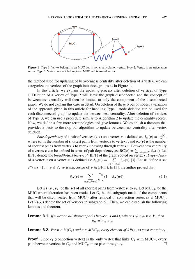
Figure 1 Type 1: Vertex belongs to an MUC but is not an articulation vertex. Type 2: Vertex is an articulationvertex. Type 3: Vertex does not belong to an MUC and is an end vertex.

the method used for updating of betweenness centrality after deletion of a vertex, we cancategorize the vertices of the graph into three groups as in Figure 1.

In this article, we explain the updating process after deletion of vertices of Type1. Deletion of a vertex of Type 2 will leave the graph disconnected and the concept ofbetweenness centrality will then be limited to only the component of the disconnectedgraph. We do not explain this case in detail. On deletion of these types of nodes, a variationof the approach given in this article for handling Type 1 node deletion can be used foreach disconnected graph to update the betweenness centrality. After deletion of verticesof Type 3, we can use a procedure similar to Algorithm 2 to update the centrality scores.Now, we define a few more terminologies and give lemmas. We establish a theorem thatprovides a basis to develop our algorithm to update betweenness centrality after vertexdeletion.

Pair dependency of a pair of vertices (s, t) on a vertex v is defined as: δst (v) = σst (v)σst

,where σst is the number of shortest paths from vertex s to vertex t , and σst (v) is the numberof shortest paths from vertex s to vertex t passing through vertex v. Betweenness centralityof a vertex v can be defined in terms of pair dependency as: BC(v) =∑

s �=v �=t∈V δst (v). LetBFTr denote the breadth-first traversal (BFT) of the graph rooted on vertex r . Dependencyof a vertex s on a vertex v is defined as: δs•(v) = ∑

t∈V \{s,v}δst (v) [3]. Let us define a set

P s(w) = {v : v ∈ V, w isasuccessor of v in BFTs}. In [3], the author proved that

δs•(v) =∑

w:v∈P s (w)

σsv

σsw

(1+ δs•(w)). (2.1)

Let SP (vi, vj ) be the set of all shortest paths from vertex vi to vj . Let MUCU be theMUC where alteration has been made. Let Gi be the subgraph made of the componentsthat will be disconnected from MUCU after removal of connection vertex ci ∈ MUCU.Let V (Gi) denote the set of vertices in subgraph Gi . Then, we can establish the followinglemmas and theorem.

Lemma 3.1. If v lies on all shortest paths between s and t , where s �= t �= v ∈ V , thenσst = σsv.σvt .

Lemma 3.2. For u ∈ V (Gk) and v ∈ MUCU , every element of SP (u, v) must contain ck .

Proof. Since ck (connection vertex) is the only vertex that links Gk with MUCU , everypath between vertices in Gk and MUCU must pass through ck .

408 GOEL ET AL.

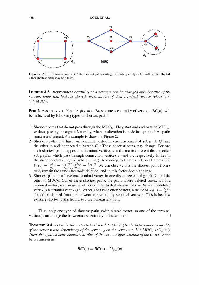
Figure 2 After deletion of vertex V 9, the shortest paths starting and ending in G5 or G7 will not be affected.Other shortest paths may be altered.

Lemma 3.3. Betweenness centrality of a vertex v can be changed only because of theshortest paths that had the altered vertex as one of their terminal vertices where v ∈V \MUCU .

Proof. Assume s, t ∈ V and s �= t �= v. Betweenness centrality of vertex v, BC(v), willbe influenced by following types of shortest paths:

1. Shortest paths that do not pass through the MUCU . They start and end outside MUCU ,without passing through it. Naturally, when an alteration is made in a graph, these pathsremain unchanged. An example is shown in Figure 2.

2. Shortest paths that have one terminal vertex in one disconnected subgraph Gi andthe other in a disconnected subgraph Gj : These shortest paths may change. For onesuch shortest path, suppose the terminal vertices s and t are in different disconnectedsubgraphs, which pass through connection vertices c1 and c2, respectively (v lies inthe disconnected subgraph where s lies). According to Lemma 3.1 and Lemma 3.2,δst (v) = σst (v)

σst= σsc1 (v).σc1c2 .σc2 t

σsc1 .σc1c2 .σc2 t= σsc1 (v)

σsc1. We can observe that the shortest paths from s

to c1 remain the same after node deletion, and so this factor doesn’t change.3. Shortest paths that have one terminal vertex in one disconnected subgraph Gi and the

other in MUCU : Out of these shortest paths, the paths where deleted vertex is not aterminal vertex, we can get a relation similar to that obtained above. When the deletedvertex is a terminal vertex (i.e., either s or t is deletion vertex), a factor of δst (v) = σst (v)

σst

should be deleted from the betweenness centrality score of vertex v. This is becauseexisting shortest paths from s to t are nonexistent now.

Thus, only one type of shortest paths (with altered vertex as one of the terminalvertices) can change the betweenness centrality of the vertex v.

Theorem 3.4. Let vd be the vertex to be deleted. Let BC(v) be the betweenness centralityof the vertex v and dependency of the vertex vd on the vertex v ∈ V \ MUCU is δvd•(v).Then, the updated betweenness centrality of the vertex v after deletion of the vertex vd canbe calculated as:

BC ′(v) = BC(v)− 2δvd•(v)


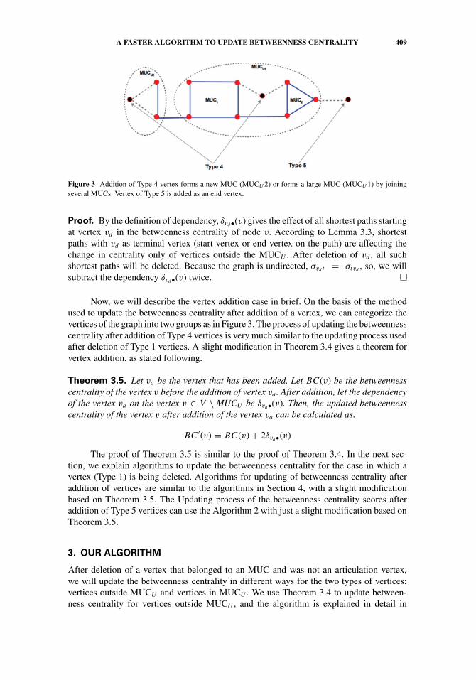
Figure 3 Addition of Type 4 vertex forms a new MUC (MUCU 2) or forms a large MUC (MUCU 1) by joiningseveral MUCs. Vertex of Type 5 is added as an end vertex.

Proof. By the definition of dependency, δvd•(v) gives the effect of all shortest paths startingat vertex vd in the betweenness centrality of node v. According to Lemma 3.3, shortestpaths with vd as terminal vertex (start vertex or end vertex on the path) are affecting thechange in centrality only of vertices outside the MUCU . After deletion of vd , all suchshortest paths will be deleted. Because the graph is undirected, σvd t = σtvd

, so, we willsubtract the dependency δvd•(v) twice.

Now, we will describe the vertex addition case in brief. On the basis of the methodused to update the betweenness centrality after addition of a vertex, we can categorize thevertices of the graph into two groups as in Figure 3. The process of updating the betweennesscentrality after addition of Type 4 vertices is very much similar to the updating process usedafter deletion of Type 1 vertices. A slight modification in Theorem 3.4 gives a theorem forvertex addition, as stated following.

Theorem 3.5. Let va be the vertex that has been added. Let BC(v) be the betweennesscentrality of the vertex v before the addition of vertex va . After addition, let the dependencyof the vertex va on the vertex v ∈ V \ MUCU be δva•(v). Then, the updated betweennesscentrality of the vertex v after addition of the vertex va can be calculated as:

BC ′(v) = BC(v)+ 2δva•(v)

The proof of Theorem 3.5 is similar to the proof of Theorem 3.4. In the next sec-tion, we explain algorithms to update the betweenness centrality for the case in which avertex (Type 1) is being deleted. Algorithms for updating of betweenness centrality afteraddition of vertices are similar to the algorithms in Section 4, with a slight modificationbased on Theorem 3.5. The Updating process of the betweenness centrality scores afteraddition of Type 5 vertices can use the Algorithm 2 with just a slight modification based onTheorem 3.5.

3. OUR ALGORITHM

After deletion of a vertex that belonged to an MUC and was not an articulation vertex,we will update the betweenness centrality in different ways for the two types of vertices:vertices outside MUCU and vertices in MUCU . We use Theorem 3.4 to update between-ness centrality for vertices outside MUCU , and the algorithm is explained in detail in

410 GOEL ET AL.

Section 3.2. When vertices in MUCU are considered, we observe that several shortestpaths that were passing through an altered vertex changed after deletion. So we recom-pute betweenness centrality using the idea given in [23], which is explained in brief inSection 3.3. We assume that the betweenness centrality score of all vertices is availablebefore proceeding with the preprocessing step of our algorithm.

3.1. Preprocessing Step

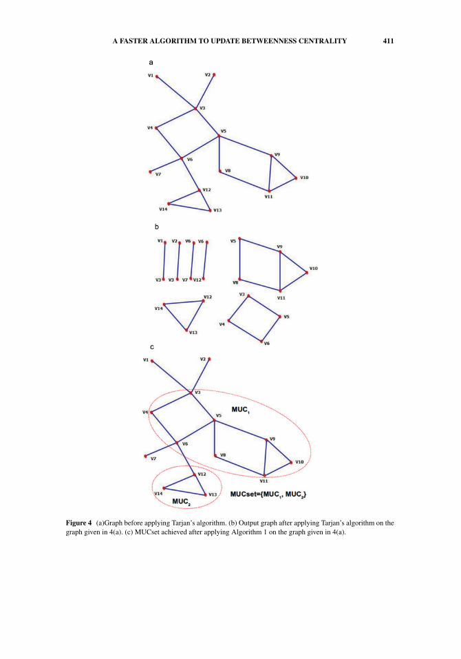
Every time a change is made in the graph, updating the MUCset becomes necessary. We cando it in two ways, either by updating the MUCset (approach used in [23]) or by recalculationof the MUCset. The approach for updatind the MUCset takes longer than recalculation.Instead of updating the MUCset, we recalculate it using the output of Tarjan’s biconnectedcomponents algorithm [38] (commonly known as Tarjan’s Algorithm). Tarjan’s biconnectedalgorithm uses the depth-first traversal of a graph for calculating biconnected components.The input to and output from Tarjan’s algorithm can be understood with the help of Figures4(a) and 4(b). The process of recalculation of the MUCset is given in Algorithm 1. The timecomplexity for calculating biconnected components is O(|V | + |E|) due to the bound ondepth-first search. Thus, the time complexity for recalculation of the MUCset (Algorithm1) is O(|V | + |E|). Following, we explain the procedure for calculating the MUCset usingbiconnected components.

Algorithm 1 Preprocessing step: Calculating MUCs in the Graph1: Use Tarjan’s Algorithm to calculate a set of biconnected components, C.2: for each Ci ∈ C do3: if |Ci | = 2 then4: Remove Ci from C.5: end if6: end for7: while ∃ Ci, Cj ∈ C where Ci and Cj have at least one common vertex do8: Remove Ci and Cj from C.9: Insert Ci ∪ Cj in C.

10: end while11: MUCset ← C

12: for each MUCj ∈ MUCset do13: Find all the connection vertices and corresponding disconnected subgraphs.14: end for

Every graph can be decomposed into a set of biconnected components, C, in whichthe elements of C are denoted by Ci (using Tarjan’s algorithm). Let |Ci | denote the numberof vertices in the biconnected component Ci . Each biconnected component contains at leastone edge (two vertices) and may share vertices (articulation vertex) with other biconnectedcomponents. We remove components that contain only one edge because a single edgecannot form an MUC. Because the elements of an MUCset are disjoint, we take repetitiveunion of the components that have at least one vertex in common. We form the MUCsetin this fashion. The MUCset generated by applying Algorithm 1 on the biconnected com-ponents (Figure 4(b)), which are calculated after applying Tarjan’s algorithm on the graphin Figure 4(a), are shown in Figure 4(c). After calculating the MUCset, for each MUC, we


Figure 4 (a)Graph before applying Tarjan’s algorithm. (b) Output graph after applying Tarjan’s algorithm on thegraph given in 4(a). (c) MUCset achieved after applying Algorithm 1 on the graph given in 4(a).

412 GOEL ET AL.

calculate connection vertices and disconnected subgraph(s) associated with each connectionvertex.

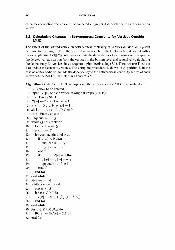
3.2. Calculating Changes in Betweenness Centrality for Vertices Outside

MUCU

The Effect of the altered vertex on betweenness centrality of vertices outside MUCU canbe found by forming BFT for the vertex that was deleted. The BFT can be calculated with atime complexity of O(|E|). We then calculate the dependency of each vertex with respect tothe deleted vertex, starting from the vertices in the bottom level and recursively calculatingthe dependency for vertices in subsequent higher levels using (3.1). Then, we use Theorem1 to update the centrality values. The complete procedure is shown in Algorithm 2. In thecase of vertex addition, we add the dependency to the betweenness centrality scores of eachvertex outside MUCU , as stated in Theorem 3.5.

Algorithm 2 Calculating BFT and updating the vertices outside MUCU accordingly1: vd : Vertex to be deleted.2: Input: BC[v] of each vertex of original graph (v ∈ V ).3: S ← Empty Stack4: P [w]←Empty List, w ∈ V

5: σ [t]← 0, t ∈ V , σ [vd ] = 16: d[t]←−1, t ∈ V , d[vd ] = 07: Q← Empty Queue8: Enqueue vd → Q

9: while Q not empty do10: Dequeue v← Q

11: push v→ S

12: for each neighbur of v do13: if d[w] < 0 then14: enqueue w→ Q

15: d[w]← d[v] + 116: end if17: if d[w] = d[v]+ 1 then18: σ [w]← σ [w]+ σ [v]19: append v→ P [w]20: end if21: end for22: end while23: δ[v]← 0, v ∈ V

24: while S not empty do25: pop w← S

26: for v ∈ P [w] do27: δ[v]← δ[v]+ σ [v]

σ [w] (1+ δ[w])28: end for29: end while30: for v ∈ V \MUCU do31: BC[v]← BC[v]− 2.δ[v]32: end for


3.3. Calculating Betweenness Centrality for Vertices in MUCU

This section briefly describes the idea suggested in [23] for recomputation of betweennesscentrality for vertices in MUCU . In the disconnected subgraph Gj , let V (Gj ) denote thevertex set and let |V (Gj )| denote the number of vertices. Let |SP (u, v)| denote the numberof shortest paths between vertex u and vertex v. Here, we will explain the basic steps ofthe algorithm, in brief. For detailed concept and the algorithm, used please refer to theQUBE algorithm [23]. Let betweenness centrality of vertex v, BC(v) for all v ∈MUCU beinitialized with 0. Let cj be a connection vertex of MUCU and Gj be the correspondingdisconnected subgraph.

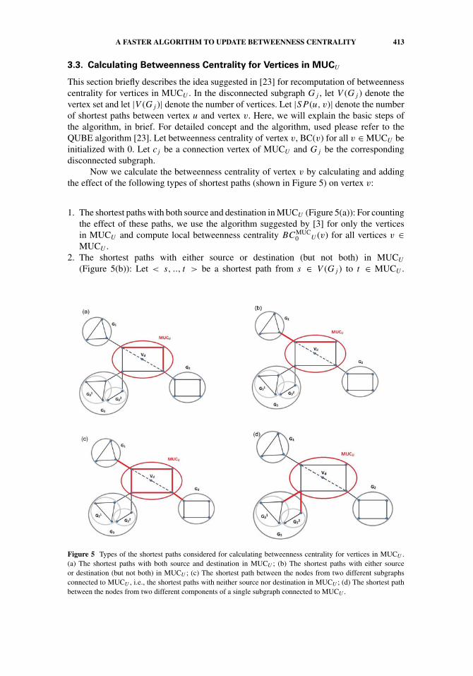
Now we calculate the betweenness centrality of vertex v by calculating and addingthe effect of the following types of shortest paths (shown in Figure 5) on vertex v:

1. The shortest paths with both source and destination in MUCU (Figure 5(a)): For countingthe effect of these paths, we use the algorithm suggested by [3] for only the verticesin MUCU and compute local betweenness centrality BCMUC

0 U (v) for all vertices v ∈MUCU .

2. The shortest paths with either source or destination (but not both) in MUCU

(Figure 5(b)): Let < s, .., t > be a shortest path from s ∈ V (Gj ) to t ∈ MUCU .

Figure 5 Types of the shortest paths considered for calculating betweenness centrality for vertices in MUCU .(a) The shortest paths with both source and destination in MUCU ; (b) The shortest paths with either sourceor destination (but not both) in MUCU ; (c) The shortest path between the nodes from two different subgraphsconnected to MUCU , i.e., the shortest paths with neither source nor destination in MUCU ; (d) The shortest pathbetween the nodes from two different components of a single subgraph connected to MUCU .

414 GOEL ET AL.

In this case, σst (v)σst= σcj t (v)

σcj t. So, to calculate the total effect of such paths, for each

shortest path < cj , ..., t >, we add the following factor to BC(v):

BC<cj ,...,t>

1 (v) =⎧⎨⎩|V (Gj )||SP (cj , t)| , if v ∈< cj , ..., vt > \{vt }0, otherwise.

3. The shortest paths with neither source nor destination in MUCU (Figures 5(c) and 5(d)):Let < s, .., t > be a shortest path from s ∈ V (Gj ) to t ∈ V (Gk) where j �= k. In this

case, σst (v)σst= σcj ck

(v)

σcj ck

. So, to calculate the total effect of such paths, for each shortest path

< cj , ..., ck >, we add the following factor to BC(v):

BC<cj ,...,ck>

2 (v) =⎧⎨⎩|V (Gj )||V (Gk)||SP (cj , ck)| , if v ∈< cj , ..., ck >

0, otherwise.

When either of the subgraphs is disconnected, an additional factor:

BCi3(ci) =

⎧⎨⎩|V (Gi)|2 −

x∑l=1

(|V (Gli)|2), if Gi is disconnected

0, otherwise.

is added to the betweenness centrality calculations (ci is a connection vertex), whereGj

l is the lth component of Gi and x is the number of connected components in Gi .

So, we have the following formula to calculate the betweenness centrality score of a vertexin MUCU :

BC(v) = BCMUCU

0 (v)+ 2∑Gj ,t

∑x∈SP (cj ,t)

BCx1(v)+

∑Gj ,Gk(j �=k)

∑y∈SP (cj ,ck)

BCy

2(v)

(+ BCi3(ci) if v = ci).

Let m be the number of edges and let n be the number of nodes in the given connected,undirected, unweighted graph with m > n. The time complexity of the proposed algorithmis O(m) when the altered vertex is an end vertex (Type 3, Type 5). In this case, we just haveto run Algorithm 2. In the other case when the altered node is of Type 1 or Type 4, the timecomplexity is O(m′n′ +m), where m′ is the number of edges and n′ is the number of nodesin MUCU ; O(m′n′) is the complexity due to the recomputation of betweenness scores of thenodes in MUCU by the traditional Brandes’ Algorithm. The additional m term in the com-plexity is due to the Algorithm 2 for updating the centrality score of vertices outside MUCU .

4. IMPLEMENTATION AND RESULTS

We have implemented the algorithm for both addition and deletion of vertices. The algorithmcan work faster for updating betweenness centrality, because it forms a subset of verticesof the graph, MUCU , for which recalculation of betweenness centrality is to be done.For the rest of the vertices, Algorithm 2 updates the betweenness centrality in negligible


time compared to the recalculation step. The recalculation procedure includes the localBrandes algorithm. So, it is directly proportional to the number of vertices inside MUCU .We have compared our results with the Brandes algorithm [3] because that is the best-known algorithm, according to our knowledge, for calculation of betweenness centralityafter vertex updating. The experiments were performed on an Intel i5-2450M CPU with2.5 GHz clock speed and 4 GB main memory.

We use a similar measure used by authors in [23] termed proportion to compare thealgorithms. Proportion can be calculated as:

(Number of vertices in MUCU

Total number of vertices in the graph

).100

Proportion is a direct function of the number of vertices in MUCU and thus speedupachieved by our algorithm is directly affected by the proportion. So, a smaller proportionwould mean that betweenness centrality for a lesser number of nodes will have to be re-computed, and this should achieve greater speedup, which we achieved in our experimentalresults. We considered the following strategy to compute the average proportion of a graph.We start randomly deleting vertices from the graph untill either the graph becomes discon-nected or k vertices are deleted. Then we take the average of proportion values for eachdeletion. The average speedup is calculated in a similar way. We consider k = 500 forreal networks. In general, average speedup on a graph or average proportion of a graphdepends on the number of MUCs formed by biconnected components and the fraction ofthe total number of vertices belonging to these MUCs. If a graph consists of most of theMUCs having small numbers of vertices with respect to the total number of vertices in thegraph, the average proportion will be small, and thus, average speedup on that graph will belarge.

4.1. Results for Synthetic Graphs

For experiments related to synthetic graphs we generated random Erdos Renyi graphs with1000, 2000, and 3000 nodes. We considered addition and deletion of nodes for differentproportions of x, for each x ∈ A, where A = {10; 20; 30; 40; 50; 60; 70; 80} in the caseof deletion and A = {10; 20; 30; 40; 50; 60; 70; 80; 90} for addition. For the experiments inwhich we considered node deletion, we used a probability of 0.05 for all generated graphs,and for experiments in which we considered node addition, we used a probability of 0.08for graphs with 1000 and 2000 nodes and 0.07 for graphs with 3000 nodes.

We initially calculated the betweenness centrality of each vertex using the Brandesalgorithm. Then we ran the preprocessing step (modified Algorithm 1 on the basis ofTheorem 3.5 for node addition and Algorithm 2 for deletion) to calculate the MUCs,connection vertices, and disconnected subgraphs for our graphs. For the case of nodedeletion, 50 vertices were continuously removed from each x proportion graph of eachgroup and average update times were calculated for different proportions. In the case ofnode addition, average updation times were calculated over 100 iterations, where, in eachiteration, a vertex was added randomly to each x proportion graph of each group.

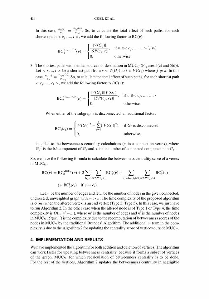
The results are plotted with average update time (in ms) at the y-axis and the pro-portion of the graphs at the x-axis for each group and are shown in Figure 6 for the vertexdeletion case and Figure 7 for the vertex addition case. We get different speedups for andifferent proportion of graphs in each group. In the case of deletion, for synthetic graphs

416 GOEL ET AL.

Figure 6 Plots for comparison of ours and the result in on synthetic graphs with 1000, 2000, and 3000 vertices,respectively, in the case of vertex deletion. (a) 1000 vertices; (b) 2000 vertices; (c) 3000 vertices.

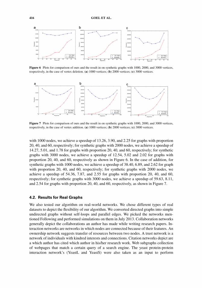
Figure 7 Plots for comparison of ours and the result in on synthetic graphs with 1000, 2000, and 3000 vertices,respectively, in the case of vertex addition. (a) 1000 vertices; (b) 2000 vertices; (c) 3000 vertices.

with 1000 nodes, we achieve a speedup of 13.26, 3.90, and 2.25 for graphs with proportion20, 40, and 60, respectively; for synthetic graphs with 2000 nodes, we achieve a speedup of14.27, 5.01, and 1.78 for graphs with proportion 20, 40, and 60, respectively; for syntheticgraphs with 3000 nodes, we achieve a speedup of 12.54, 5.02 and 2.02 for graphs withproportion 20, 40, and 60, respectively as shown in Figure 6. In the case of addition, forsynthetic graphs with 1000 nodes, we achieve a speedup of 38.40, 6.89, and 2.62 for graphwith proportion 20, 40, and 60, respectively; for synthetic graphs with 2000 nodes, weachieve a speedup of 54.36, 7.87, and 2.55 for graphs with proportion 20, 40, and 60,respectively; for synthetic graphs with 3000 nodes, we achieve a speedup of 59.63, 8.11,and 2.54 for graphs with proportion 20, 40, and 60, respectively, as shown in Figure 7.

4.2. Results for Real Graphs

We also tested our algorithm on real-world networks. We chose different types of realdatasets to depict the flexibility of our algorithm. We converted directed graphs into simpleundirected graphs without self-loops and parallel edges. We picked the networks men-tioned Following and performed simulations on them in July 2013. Collaboration networksgenerally depict the collaborations an author has made while writing research papers. In-teraction networks are networks in which nodes are connected because of their features. Anownership network suggests transfer of resources between two nodes. A trust network is anetwork of individuals with kindred interests and connections. Citation networks depict area which author has cited which author in his/her research work. Web subgraphs collectionof webpages that match a certain query of a search engine. The yeast protein-proteininteraction network’s (YeastL and YeastS) were also taken as an input to perform


Avg. Avg.Name of Dataset Type |V| |E| Proportion Speed-up

YeastL Interaction 2361 6646 31.16 64.88YeastS Interaction 2361 6646 28.05 72.76Geom Collaboration 7343 11898 17.08 7.63Erdos02 Collaboration 6927 11850 7.13 323.75Edros972 Collaboration 5488 8972 9.49 411.835ODLIS Dictionary data 2909 16377 67.68 18.52Wiki-vote Trust 7115 100762 38.452 28.472California Web Subgraphs 9664 15969 25.54 77.658EPA Web Subgraphs 4772 8909 21.55 150.456Lederberg Citation 8843 41532 58.86 45.159SciMet Citation 3084 10399 62.42 17.55US Power Grid Electronic Transport 4941 6594 38.03 35.42

Table I Simulation results for real-world datasets.

simulations.3 We picked Geom, Erdos02, Erdos972, California, EPA, Lederberg, SciMetand US Power Grid networks.4 ODLIS network.5 weblink. We also extracted Wiki-vote net-work.6 For the real networks mentioned, information about networks, average proportion,and average speed-ups over the Brandes algorithm are summarized in Table I.

5. RELATED WORK

The idea of betweenness centrality was first introduced in articles by [1, 10]. In article[31], another measure, which considered random walks on any arbitrary length rather thanjust shortest paths between two vertices, was defined. In [4], other types of betweennesscentrality such as, edge betweenness and group betweenness and algorithms to computethem efficiently were considered. Betweenness centrality was earlier calculated by find-ing the number and length of shortest paths between two vertices and then adding pairdependencies for all pairs. An algorithm was suggested in [3], which introduces a re-cursive way to sum the dependencies in graphs. Although the algorithm proposed in [3]was faster than that used previously, it was still too costly for large graphs. Recently,[32] gave an approach that could reduce the betweennesss computation based on somespecial structures in graphs such as several small biconnected components and severalisomorphic nodes (nodes with the same neighburhood). Several approximation algorithmswere proposed [2, 6, 11, 26]. Real-world networks tend to be large and transient. Workhas been done in [23, 12] to find betweenness centrality after updating in a graph. Thealgorithm suggested in [23] selects a subset of vertices whose betweenness centrality isupdated. However, it works only in the case of edge removal and addition. The algorithm

3The data for YeastL and Yeast S is available at http://vlado.fmf.unilj.si/pub/networks/data/bio/Yeast/ Yeast.htm website

4http://www.cise.ufl.edu/research/sparse/matrices/Pajek/5http://vlado.fmf.uni-lj.si/pub/networks/data/dic/odlis/Odlis.htm6http://snap.stanford.edu/data/wiki-Vote.html

418 GOEL ET AL.

suggested in [12] takes into consideration different instances that might arise due to edgeaddition in a graph and speeds up the algorithm in these cases. This algorithm works onlyfor streaming graphs, i.e., only in the case of edge additions. Recently, in an article [29],an incremental algorithm for updating edges using Single Source Shortest Path DirectedAcyclic Graphs for each vertex was used recursively to update vertices. They have reportedthe time complexity for updating to O(m′n + n2), where m′ is the maximum number ofedges that can lie on a shortest path. Another incremental algorithm was given in [20],which extends the incremental algorithm for finding the all pairs shortest path problem. Re-cently, several other algorithms [39, 13, 22] have been proposed that speedup the updatingprocess of betweenness centrality and [39]. algorithms for updating closeness centrality .Those algorithms work in two steps: convergence and aggregation. In the convergence step,the authors calculate the difference in the number of shortest paths or the difference in thelength’s of shortest paths before and after updating. Then, they aggregate the changes in theexisting centrality scores to get the updated centrality in the aggregation step. In anotherstudy [22], an online algorithm is given that can keep the betweennesss of nodes and edgesup to date. [13] A distributed approach for updating the betweenness score in the distributedonline social networks is given.

6. CONCLUSION

In this article, we formulated an algorithm that efficiently calculates betweenness centralitywhen vertices in a graph are updated. We did not consider the traditional way of updatingbetweenness centrality after node alteration, which considers a node alteration event asa series of edge alteration event’s. We achieved the speedups by calculating two sets ofvertices; one for which we need to update betweenness scores and the other for which weneed to recompute the betweenness score. We achieve an average speedup of 6.13 for aproportion of 40 for considered synthetic graphs compared to the Brandes algorithm [3].For real graphs, we get an average speedup of around 133 for a proportion of 29. Thespeedup will increase further when proportion decreases.

REFERENCES

[1] J. M. Anthonisse “The Rush in a Directed Graph.” Stichting Mathematisch Centrum. Mathe-matische Besliskunde BN 9/71(1971):1–10.

[2] D. A. Bader, S. Kintali, K. Madduri, and M. Mihail. “Approximating Betweenness Centrality.” InProceedings of the 5th International Conference on Algorithms and Models for the Web-Graph,WAW’07, pp. 124–137. Berlin, Heidelberg: Springer-Verlag, 2007.

[3] U. Brandes. “A Faster Algorithm for Betweenness Centrality.” The Journal of MathematicalSociology 25:2 (2001),163–177.

[4] U. Brandes. “On Variants of Shortest-Path Betweenness Centrality and Their Generic Compu-tation.” Social Networks 30:2 (2008),136–145.

[5] U. Brandes and T. Erlebach (Editors). Network Analysis: Methodological Foundations, LNCS3418. Berlin, Heidelberg: Springer, 2005.

[6] U. Brandes and C. Pich. “Centrality Estimation in Large Networks.” International Journal ofBifurcation and Chaos 17:07 (2007), 2303–2318.

[7] R. Carvalho, L. Buzna, F. Bono, E. Gutierrez, W. Just, and D. Arrowsmith. “Robustness ofTrans-European Gas Networks.” Physical review E 80:1 (2009), 016106.

[8] S. Derrible. “Network Centrality of Metro Systems.” PloS One 7:7 (2012), e40575.


[9] A. Flrez, D. Park, J. Bhak, B.-C. Kim, A. Kuchinsky, J. Morris, J. Espinosa, and C. Muskus.“Protein Network Prediction and Topological Analysis in Leishmania Major as a Tool for DrugTarget Selection.” BMC Bioinformatics 11:1 (2010), 1–9.

[10] L. C. Freeman. “A Set of Measures of Centrality Based on Betweenness.” Sociometry 40:1(1977), 35–41.

[11] R. Geisberger, P. Sanders, and D. Schultes. “Better Approximation of Betweenness Centrality.”In Proceedings of 10th Workshop on ALENEX, pp. 90–100. SIAM, 2008.

[12] O. Green, R. McColl, and D. Bader. “A Fast Algorithm for Streaming Betweenness Central-ity." In 2012 International Conference on Privacy, Security, Risk and Trust (PASSAT), and2012 International Conference on Social Computing (SocialCom), pp. 11–20. ASE/IEEE,(2012).

[13] B. Guidi, M. Conti, A. Passarella, and L. Ricci. “Distributed Protocols for Ego BetweennessCentrality Computation in DOSNs.” In 2014 IEEE International Conference on PervasiveComputing and Communications Workshops (PERCOM Workshops), pp. 539–544. IEEE,2014.

[14] P. Hage, and F. Harary. “Eccentricity and Centrality in Networks.” Social Networks 17:1(1995),57–63.

[15] A. Hanna. “Revolutionary Making and Self-Understanding: The Case of #Jan25 and SocialMedia Activism.” Paper presented at meeting of the International Studies Association, SanDiego , CA, April 2012.

[16] Y. J. Huang, D. Hang, L. J. Lu, L. Tong, M. B. Gerstein, and G. T. Montelione. Targetingthe human cancer pathway protein interaction network by structural genomics. Molecular &Cellular Proteomics 7:10 (2012), 2048–2060.

[17] Y. Iturria-Medina, R. C. Sotero, E. J. Canales-Rodrıguez, Y. Aleman-Garcıa, and L. Melie-Gomez. “Studying the Human Brain Anatomical Network via Diffusion-Weighted MRI AndGraph Theory.” Neuroimage 40:3 (2008), 1064–1076.

[18] M. O. Jackson. Social and Economic Networks. Princeton, NJ, USA: Princeton UniversityPress, 2008.

[19] M. P. Joy, A. Brock, D. E. Ingber, and S. Huang. “High-Betweenness Proteins in the YeastProtein Interaction Network.” BioMed Research International 2005:2 (2005), 96–103.

[20] M. Kas, M. Wachs, K. M. Carley, and L. R. Carley. “Incremental Algorithm for UpdatingBetweenness Centrality in Dynamically Growing Networks.” In Proceedings of the 2013IEEE/ACM International Conference on Advances in Social Networks Analysis and Mining,ASONAM ’13, pp. 33–40. New York, NY, USA. ACM, 2005.

[21] T. Kavitha, K. Mehlhorn, D. Michail, and K. Paluch. “A Faster Algorithm for Minimum CycleBasis of Graphs.” In Automata, Languages and Programming, edited by J. Daz, J. Karhumki,A. Lepist, and D. Sannella, pp. 846–857, Lecture Notes in Computer Science 3142. Berlin,Heidelberg: Springer, 2004.

[22] N. Kourtellis, G. D. F. Morales, and F. Bonchi. “Scalable Online Betweenness Centrality inEvolving Graphs.” arXiv preprint arXiv:1401.6981, 2014.

[23] M.-J. Lee, J. Lee, J. Y. Park, R. H. Choi, and C.-W. Chung. “Qube: A Quick Algorithm forUpdating Betweenness Centrality.” In Proceedings of the 21st International Conference onWorld Wide Web, WWW ’12, pp. 351–360. New York, NY, USA. ACM, 2012.

[24] J. Lienert, F. Schnetzer, and K. Ingold. “Stakeholder Analysis Combined with Social NetworkAnalysis Provides Fine-Grained Insights into Water Infrastructure Planning Processes.” Journalof Environmental Management 125 (2013), 134–148.

[25] T.-C. Lu, Y. Zhang, D. L. Allen, and M. A. Salman. “Design for Fault Analysis UsingMulti-Partite, Multi-Attribute Betweenness Centrality Measures.” In Proceedings of the An-nual Conference of the Prognostics and Health Management Society 2011, pp. 190–197. PHM,2011.

[26] Y. Makarychev. “Simple Linear Time Approximation Algorithm for Betweenness.” OperationsResearch Letters 40:6 (2012), 450–452.

420 GOEL ET AL.

[27] Y. Nagata, K. Asatani, and H. Otsuka. “A New Load-Balancing Method Applying Link-CostAdjustment Based on Betweenness Centrality in WDM Networks.” In Proc. of the 6th Interna-tional Conference on Ubiquitous and Future Networks (ICUFN), pp. 59–60. IEEE, 2014.

[28] S. Narayanan. “The Betweenness Centrality of Biological Networks.” PhD thesis, VirginiaPolytechnic Institute and State University, 2005.

[29] M. Nasre, M. Pontecorvi, and V. Ramachandran. “Betweenness Centrality–Incremental andFaster.” arXiv preprint arXiv:1311.2147, 2013.

[30] M. Newman. Networks: An Introduction. New York, NY, USA: Oxford University Press, 2010.[31] M. J. Newman “A Measure Of Betweenness Centrality Based On Random Walks.” Social

Networks, 27:1 (2005), 39–54.[32] R. Puzis, Y. Elovici, P. Zilberman, S. Dolev, and U. Brandes. “Topology Manipulations for

Speeding Betweenness Centrality Computation.” Journal of Complex NetWorks. Availableonline (http://comnet.oxfordjournals.org/content/early/2014/04/29/comnet.cnu015.abstract),2014.

[33] G. Sabidussi. “The Centrality Index of a Graph.” Psychometrika 31:4(1966), 581–603.[34] J. Scheurer and C. Curtis. “Spatial Network Analysis of Multimodal Transport Systems: Devel-

oping a Strategic Planning Tool to Assess the Congruence of Movement and Urban Structure: aCase Study of Perth Before and After the Perth-to-Mandurah Railway.” GAMUT, AustralasianCentre for the Governance and Management of Urban Transport, University of Melbourne,2008.

[35] B. Shanmugham and A. Pan. “Identification and Characterization of Potential TherapeuticCandidates in Emerging Human Pathogen Mycobacterium Abscessus: A Novel Hierarchical inSilico Approach.” PloS One, 8:3 (2013), e59126.

[36] A. Shimbel. “Structural Parameters of Communication Networks.” The Bulletin of MathematicalBiophysics 15:4 (1953), 501–507.

[37] T. Spiliotopoulos and I. Oakley. “Applications of Social Network Analysis for User Modeling.”In Proceedings of the International Workshop on User Modeling from Social Media. New York,NY, USA: ACM, 2012.

[38] R. Tarjan. “Depth-First Search and Linear Graph Algorithms.” SIAM Journal on Computing,1:2 (1972), 146–160.

[39] W. Wei and K. Carley. “Real Time Closeness and Betweenness Centrality Calculationson Streaming Network Data.” Paper presented at the Proceedings of the 2014 ASE Big-Data/SocialCom/Cybersecurity Conference, Stanford University, May 27–31, 2014.

[40] Y. Yan, L. Xiao, and Z. Xintian. “Analyzing and Identifying of Cascading Failure in SupplyChain Networks.” In Proceedings of the 2010 International Conference on Logistics Systemsand Intelligent Management 3 (2010), pp.1292–1295.

[41] H. Yu, P. M. Kim, E. Sprecher, V.Trifonov, and M. Gerstein. “The Importance of Bottlenecksin Protein Networks: Correlation with Gene Essentiality and Expression Dynamics.” PLoSComputational Biology 3:4 (2007), e59.

a faster algorithm to update betweenness centrality …

Documents