a finite field framework for modeling, analysis and … article (for engineering journals) a finite...
TRANSCRIPT
Draft Article (For Engineering Journals)
A Finite Field Framework for Modeling, Analysis and Control
of Finite State Automata
JOHANN REGER†,1 AND KLAUS SCHMIDT‡
SUMMARY
In this paper we address the modeling, analysis and control of finite state automata, which represent astandard class of discrete event systems. As opposed to graph theoretical methods we consider an algebraicframework that resides on the finite fieldF2, which is defined on a set of two elements with the operationsaddition and multiplication, both carried out modulo 2. Thekey characteristic of the model is its functionalcompleteness in the sense that it is capable of describing most of the finite state automata in use, includingnon-deterministic and partially defined automata. Starting from a graphical representation of an automatonand applying techniques from boolean algebra we derive the transition relation of our finite field model. Forcases, in which the transition relation is linear, we develop means for treating the main issues in the analysisof the cyclic behavior of automata. This involves the computation of the elementary divisor polynomialsof the system dynamics, and the periods of these polynomials, which are shown to completely determinethe cyclic structure of the state space of the underlying linear system. Dealing with non-autonomous linearsystems with inputs, we use the notion of feedback in order tospecify a desired cyclic behavior of theautomaton in the closed loop. The computation of an appropriate state feedback is achieved by introducingan image domain and adopting the well-established polynomial matrix method to linear discrete systemsover the finite fieldF2. Examples illustrate the main steps of our method.
Keywords: Finite State Automata, Linear Modular Systems, Finite Fields.
1. INTRODUCTION
In the world of continuous dynamic systems, state space models are the dominantparadigm of representing a system algebraically. It is due to this algebraic setting thatmost of the real world system properties can be retrieved in the algebraic model, sincethe algebra entails a certain structural framework. In contrast to continuous systems,discrete event systems characteristically show a lack of structure, that is, these systems
1Address correspondance to: Johann Reger, Lehrstuhl fur Regelungstechnik, Friedrich-Alexander-Universitat Erlangen-Nurnberg, Cauerstraße 7, 91058 Erlangen, Germany.†Erlangen-Nuremberg University, Institute of Automatic Control, Department of Electrical, Electronic andCommunication Engineering, Erlangen, Germany.
‡Carnegie Mellon University, Department of Electrical and Computer Engineering, Pittsburgh, USA.
J. REGER AND K. SCHMIDT 2
do not fit naturally into an algebraic frame since many of the real world properties canhardly be captured in some nice algebraic structures, as do eigenvalues, for example,when dealing with stability issues in linear continuous systems theory. However, a lotof effort has been made to setup a link between both classes ofsystems.
In search of analogies to linear continuous systems, state space models using so-calledarithmetical polynomialshave been introduced for representing finite state au-tomata [4, 3]. A second method employsWalsh functionsto model deterministic fi-nite state automata as autonomous linear systems [10]. As pointed out in [13], thecrucial drawbacks, which are common in both approaches, arethe absence of suffi-cient and efficient criteria for an algebraic locating of theinherent cyclic propertiesof automata. Even for linear systems the former approach only provides necessarycriteria, whereas the latter runs into numerical difficulties by enumerating the wholestate space. Another severe problem is the computational complexity, as within theseapproaches solving for certain cyclic states is of non-polynomial complexity (NP-complete). This is due to the fact that the associated algebraic operations do not con-stitute a group because they are not closed under the operation sets. Unfortunately,there is no polynomial time algorithm that solves a linear system of equations over therational numbers for boolean vectors. As a consequence, NP-completeness impliesthat any problem in practice is rendered intractable.
In contrast to the approaches from above, the model to be developed in this paperis capable of overcoming these obstacles. To this end, we consider an algebraic statespace description that is formulated strictly in (modulo 2-) operations on the set ofboolean numbers, mathematically speaking, we operate on a finite field F2.1 Thus,contrary to the afore-mentioned approaches, we can benefit from the field property;at least in the linear case, it is possible to solve for cyclicstates in polynomial time.Despite some peculiarities of finite fields, it will turn out that if one is concernedwith state space modeling of automata, finite fields provide those algebraic conceptsthat are necessary for relating automata properties to structural, algebraic properties.This leads to a sufficient and efficient analysis of the cyclicbehavior of deterministicand non-deterministic finite state automata, especially inthe linear case. In this case,the key concepts are given by the notions of invariant polynomials and the periodof a polynomial, which will be shown to grant the statement ofsufficient criteria fordetermining all cycles of a deterministic linear automaton, in multiplicity and length.
Based on this knowledge the synthesis of linear state feedback for imposing prop-erties on the controlled linear system with respect to cyclic states is carried out. Wedemonstrate that this amounts to setting the (invariant) elementary divisor polyno-
1Finite field models have already been under consideration inthe control community [5]. Still, neitherwere finite fields utilized for determining the cyclic structure of automata nor were any analogies drawnto continuous time systems. On the other hand much of the theory was already developed as early as thesixties — for instance the design of linear feedback shift registers [7, 6] — but has not been adapted forcontrol purposes yet.

3 A FINITE FIELD FRAMEWORK FOR FINITE STATE AUTOMATA
mials of the closed loop dynamics. In the scope of continuoussystems, resorting tostandard methods as for example employing the parametric approach [15], this is adifficult task to perform — we comment on that in detail. Instead, we propose an im-age domain method for linear discrete systems [14], an adaption of the polynomialmatrix method [11], in which our synthesis goal of setting the invariant polynomialsapparently proofs to be more practicable. This results in analgorithm for generat-ing a linear state feedback which fits a given linear automaton with specified cyclicproperties. Additionally, the algorithm meets the requirements burdened by structuralconstraints, as stated in Rosenbrock’s structure theorem [11].
The outline of the paper is as follows: Section 2 introduces the minimum necessaryalgebraic terminology. Section 3 exposes, in an exemplary fashion, two methods forobtaining a multilinear automaton model over the finite fieldF2 by referring to ele-mentary boolean algebra. In Section 4 we are concerned with the analysis of lineardiscrete models overF2. Taking advantage of the notion of feedback we show how toimpose structural properties on closed loop systems in Section 6. Finally, in Section 7we recall the main ideas and give some hints in view of extending the setting.
2. ALGEBRAIC PRELIMINARIES
Linear algebra over the fields of real and complex numbers is awidely spread toolall over the engineering sciences. On the contrary, except from signal processing andcoding theory, discrete mathematics and finite fields are encountered quite rarely inthe academic education of engineers. On this account, the most important conceptualterms from algebra which represent the bases for our automaton model in view (Sec-tion 3) are recapitulated in the sequel. Some remarks spot the differences betweenfinite and infinite fields. We refer to the comprehensive and thorough introduction tofinite fields by Lidl and Niederreiter [12].
2.1. Finite FieldsDefinition 1 (Group)A group is a setG together with a binary operation∗ such that
1. For alla,b∈ G, a∗b∈ G.2. The operation∗ is associative, i. e.a∗ (b∗ c) = (a∗b)∗ c for anya,b,c∈ G.3. An identity element,e∈ G, exists such that for alla∈ G, a∗e= e∗a = a.4. For anya∈ G an inverse elementa−1 ∈ G exists such thata∗a−1 = a−1∗a = e.
Moreover, a group is commutative (or abelian) if for alla,b∈ G, a∗b= b∗a. A groupis called finite if the setG contains finitely many elements.

J. REGER AND K. SCHMIDT 4
As we will make abundant use of polynomials in the subsequentsections we need todefine the notion of a ring.
Definition 2 (Ring)A ring is a setR together with two binary operations, addition + and multiplication· ,such that
1. R is a commutative group with respect to addition.2. Multiplication is associative , i. e.a · (b ·c) = (a ·b) ·c for anya,b,c∈R.3. R is distributive with respect to addition and multiplication, that is
a · (b+c) = a ·b+a ·cand(b+c) ·a= b ·a+c ·a for all a,b,c∈R.
A ring is called commutative if its multiplication is commutative.
The setR of polynomials in the independent variableλ with the usual addition andmultiplication of polynomials forms a ring, the ring of polynomials denoted byR[λ].
It is essential for a ring that a multiplicative inverse neednot exist in general. Inorder to be able to solve for multiplicatively bound indeterminates it is helpful toincrease the requirements by excluding the critical element from the set.
Definition 3 (Field)A ring on a setF with the operations addition an multiplication, + and· , is a fieldif the subsetF \{0} is a commutative group with respect to multiplication. A field F
with q elements, denoted byFq, is called finite ifq is finite.
In further sections of the paper a special type of field is utilized that is based on thedivision remainder operationmodulo.
Definition 4 (Galois-Field)The set of integers{0,1, . . . ,q−1}, whereq is a prime number, with the operationsaddition and multiplication moduloq, is a finite field, called Galois-FieldFq.
The primality ofq is decisive for the existence of a multiplicative inverse element.Otherwise zero divisors would occur (for instance 2·3 modulo 6= 0, henceF6 is nota field ). In the sequel,Fq will always denote a Galois Field and beginning with Section3 we will concentrate on Galois-Fields fieldsF2 only. Consequently, fora,b∈ F2
a+b := a+b mod 2,a ·b := a ·b mod 2.
Note that in this case subtraction modulo 2 coincides with addition modulo 2.
Theorem 1 (Fermat’s Little Theorem)Let q∈ Z be a prime number. Then for all integersλ, which are not divisible byq, qdividesλq−1−1.

5 A FINITE FIELD FRAMEWORK FOR FINITE STATE AUTOMATA
Consequently, everyλ ∈ Fq satisfiesλq = λ. Hence, a polynomialp ∈ Fq[λ] can beidentical to zero for arbitraryλ ∈ Fq, sincep may contain polynomialsλq−λ, whichare identical to zero. In contrast to finite fields, a polynomial p∈ R[λ] over the infinitefield of real numbersR is identical to zero if and only if all coefficients are zero.
2.2. Polynomials over Finite Fields
According to Gauß’ fundamental theorem of algebra, a fundamental property of poly-nomials is that all polynomials over the field of real numbersR can be factorized(reduced) in quadratic factors inR[λ], or over the extension fieldC even more in lin-ear factors inC[λ]. Naturally one would expect that this holds true for finite fields aswell. We will see that for finite fieldsFq, in general, this is not the case.
Factorization of Polynomials
Definition 5 (Monic Polynomial)A polynomialp(λ) = ∑d
i=0ai λi with degreed is called monic ifad = 1.
Definition 6 (Irreducible Polynomial)A non-constant polynomialp∈ F[λ] is called irreducible overF if wheneverp(λ) =g(λ)h(λ) in F[λ] then eitherg(λ) or h(λ) is a constant.
In view of irreducibility we can rephrase Gauß’ fundamentaltheorem of algebra.
Theorem 2 (Unique Factorization Theorem)Any polynomialp∈ F[λ] can be written in the form
p = a p1e1 · · · pk
ek , (1)
wherea∈ F, p1, . . . , pk ∈ F[λ] are distinct polynomials that are irreducible overF, ande1, . . . ,ek ∈ N. This factorization is unique apart from the sequence of thefactors.
For the fieldR all polynomialspi in Theorem 2 are of degreeei ≤ 2. This does notapply for finite fields, for example:p(λ) = λ5 + λ2 + λ + 1 = (λ3 + λ + 1)(λ + 1)2,p ∈ F2[λ], becauseλ3 + λ + 1 andλ + 1 are irreducible overF2. Another propertywhich is peculiar to finite fields is the periodicity property.
Period of Polynomials
Definition 7 (Period of a Polynomial)Let p ∈ Fq[λ] be a non-zero polynomial. Ifp(0) 6= 0, then the least positive integerτ for which p(λ) dividesλτ − 1 is called the period (order) of the polynomialp. Ifp(0) = 0, thenp(λ) = λhg(λ), whereh ∈ N andg ∈ Fq[λ] with g(0) 6= 0, andτ isdefined as the period ofg.
J. REGER AND K. SCHMIDT 6
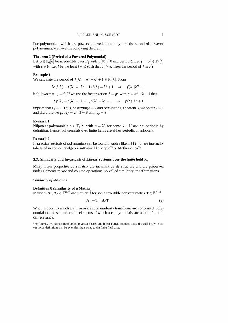
For polynomials which are powers of irreducible polynomials, so-called poweredpolynomials, we have the following theorem.
Theorem 3 (Period of a Powered Polynomial)Let p∈ Fq[λ] be irreducible overFq with p(0) 6= 0 and periodτ. Let f = pe ∈ Fq[λ]
with e∈ N. Let l be the leastl ∈ Z such thatql ≥ e. Then the period off is ql τ.
Example 1We calculate the period off (λ) = λ4 + λ2+1∈ F2[λ]. From
λ2 f (λ)+ f (λ) = (λ2 +1) f (λ) = λ6 +1 ⇒ f (λ)|λ6 +1
it follows thatτ f = 6. If we use the factorizationf = p2 with p = λ2 + λ +1 then
λ p(λ)+ p(λ) = (λ +1)p(λ) = λ3 +1 ⇒ p(λ)|λ3 +1
implies thatτp = 3. Thus, observinge= 2 and considering Theorem 3, we obtainl = 1and therefore we getτ f = 21 ·3 = 6 with τp = 3.
Remark 1Nilpotent polynomialsp ∈ Fq[λ] with p = λk for somek ∈ N are not periodic bydefinition. Hence, polynomials over finite fields are either periodic or nilpotent.
Remark 2In practice, periods of polynomials can be found in tables like in [12], or are internallytabulated in computer algebra software like MapleR© or MathematicaR©.
2.3. Similarity and Invariants of Linear Systems over the finite field Fq
Many major properties of a matrix are invariant by its structure and are preservedunder elementary row and column operations, so-called similarity transformations.2
Similarity of Matrices
Definition 8 (Similarity of a Matrix)MatricesA1, A2 ∈ F
n×n are similar if for some invertible constant matrixT ∈ Fn×n
A1 = T−1A2T . (2)
When properties which are invariant under similarity transforms are concerned, poly-nomial matrices, matrices the elements of which are polynomials, are a tool of practi-cal relevance.2For brevity, we refrain from defining vector spaces and linear transformations since the well-known con-ventional definitions can be extended right away to the finitefield case.

7 A FINITE FIELD FRAMEWORK FOR FINITE STATE AUTOMATA
Theorem 4 (Smith Form of the Characteristic Matrix)For anyA ∈ Fn×n, polynomial matricesU(λ),V(λ) with non-zero determinant inde-pendent fromλ exist such that
U(λ)(λI −A)V(λ) = S(λ), S(λ) = diag(c1(λ), . . . ,cn(λ)
)(3)
in which the monic polynomialsci+1|ci , i = 1, . . . ,n−1. The polynomial matrixS(λ)is called the Smith (normal) form of (the characteristic matrix wrt.) A.
Matrices are similar iff they have the same Smith form. As thepolynomialsci , i =1, . . . ,n are preserved under similarity transforms this gives rise to define invariants.
Invariant Polynomials
Definition 9 (Invariant polynomials)The unique non-constant monic polynomialsci(λ), i = 1, . . . ,n, referring to the Smithform S(λ) of a matrixA, are the invariant polynomials (similarity invariants) ofA.
The uppermost polynomialc1(λ) is the minimal polynomial of the matrixA. Theproduct of all invariant polynomials is its characteristicpolynomial det(λI −A).
Definition 10 (Elementary Divisor Polynomials)Let ci ∈ F[λ], i = 1, . . . ,n, be the invariant polynomials of a matrixA and letci =
pei,1i,1 · · · pei,Ni
i,Niwith Ni ∈ N be the unique factorization ofci due to Theorem 2. Then, the
N = ∑ni=1Ni non-constant factor polynomialsp
ei, ji, j , i = 1, . . . ,n and j = 1, . . . ,Ni , are
termed elementary divisor polynomials ofA.
The Rational Canonical Form
In addition to the Smith form (3), we will use a normal form referring to the elementarydivisor polynomials. This will involve the notion of a companion matrix.
Definition 11 (Companion Matrix)Let p(λ) = ∑d
i=0aiλi ∈ F[λ] be a monic polynomial of degreed. The matrixC∈ Fd×d
C =
0 1 0 · · · 0 00 0 1 · · · 0 0...
......
. . ....
...0 0 0 · · · 0 1
−a0 −a1 −a2 · · · −ad−2 −ad−1
(4)
is called the companion matrix with respect to the polynomial p(λ).
Companion matrices have some useful properties, e. g. its characteristic polynomialcoincides with its minimal polynomial, which is just the defining polynomialp(λ).

J. REGER AND K. SCHMIDT 8
Theorem 5 (Rational Canonical Form)For anyA ∈ Fn×n there exists a similarity transformT by virtue of which
Arat = TAT −1, Arat = diag(C1, . . . ,CN) (5)
with j = 1, . . . ,N companion matricesC j defined by theN elementary divisor poly-nomials ofA. The matrixArat is unique up to block ordering and is called (elementarydivisor form of the) rational canonical form or classical canonical form ofA.
Example 2For the following Smith form of a matrixA ∈ F
6×62 ,
S(λ) = diag((λ2 + λ +1)(λ +1)2λ,λ +1,1,1,1,1
)
we have the elementary divisor polynomials
p1(λ) = λ2 + λ +1, p2(λ) = (λ +1)2, p3(λ) = λ, p4(λ) = λ +1.
defining the companion matrices in the rational canonical form of A, that is
C1 =
(0 11 1
)
, C2 =
(0 11 0
)
, C3 =(0), C4 =
(1), Arat = diag(C1,C2,C3,C4) .
Remark 3We did not introduce the Jordan normal form of a matrix, whichwould follow fromdiagonalizing the rational canonical form. The reason is that the Jordan normal formis accompanied by the notion of an extension fieldFqk,k = 1,2, . . . associated toFq. Incase of a finite field, the calculation of roots in this extension fieldFqk is much morecumbersome than it is in the extension field associated to thereal numbersR, whichis C, the field of complex numbers.
3. MULTILINEAR AUTOMATON MODEL OVER THE FINITE FIELD F2
In this section we develop an algebraic model for a non-deterministic finite state au-tomaton with multiple inputs. It takes the form
f (x[k+1],x[k],u[k]) = 0, x ∈ Fn2, u ∈ F
m2 , (6)
where f marks an implicit scalar transition functionf : Fn2×Fn
2×Fm2 → F2, which
relates then statesx[k] and them inputsu[k] in an instantk with the possibly multiplesuccessor statesx[k+1] in the instantk+1, indicating possible behavior by mappingonto 0. The transition function is multilinear in the vectorelements ofx[k+1], x[k] andu[k] except for a constant. This will be shown subsequently.
9 A FINITE FIELD FRAMEWORK FOR FINITE STATE AUTOMATA
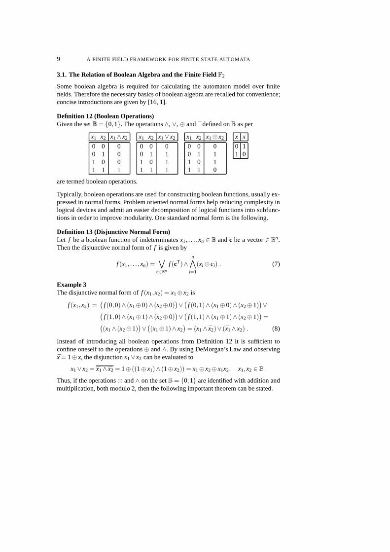
3.1. The Relation of Boolean Algebra and the Finite FieldF2
Some boolean algebra is required for calculating the automaton model over finitefields. Therefore the necessary basics of boolean algebra are recalled for convenience;concise introductions are given by [16, 1].
Definition 12 (Boolean Operations)Given the setB = {0,1}. The operations∧, ∨, ⊕ and ¯ defined onB as per
x1 x2 x1∧x2
0 0 00 1 01 0 01 1 1
x1 x2 x1∨x2
0 0 00 1 11 0 11 1 1
x1 x2 x1⊕x2
0 0 00 1 11 0 11 1 0
x x
0 11 0
are termed boolean operations.
Typically, boolean operations are used for constructing boolean functions, usually ex-pressed in normal forms. Problem oriented normal forms helpreducing complexity inlogical devices and admit an easier decomposition of logical functions into subfunc-tions in order to improve modularity. One standard normal form is the following.
Definition 13 (Disjunctive Normal Form)Let f be a boolean function of indeterminatesx1, . . . ,xn ∈ B andc be a vector∈ B
n.Then the disjunctive normal form off is given by
f (x1, . . . ,xn) =_
c∈Bn
f (cT)∧n
i=1
(xi ⊕ci) . (7)
Example 3The disjunctive normal form off (x1,x2) = x1⊕x2 is
f (x1,x2) =(
f (0,0)∧ (x1⊕0)∧ (x2⊕0))∨(
f (0,1)∧ (x1⊕0)∧ (x2⊕1))∨
(f (1,0)∧ (x1⊕1)∧ (x2⊕0)
)∨(
f (1,1)∧ (x1⊕1)∧ (x2⊕1))=
((x1∧ (x2⊕1)
)∨((x1⊕1)∧x2
)= (x1∧ x2)∨ (x1∧x2) . (8)
Instead of introducing all boolean operations from Definition 12 it is sufficient toconfine oneself to the operations⊕ and∧. By using DeMorgan’s Law and observingx = 1⊕x, the disjunctionx1∨x2 can be evaluated to
x1∨x2 = x1∧ x2 = 1⊕ ((1⊕x1)∧ (1⊕x2)) = x1⊕x2⊕x1x2, x1,x2 ∈ B .
Thus, if the operations⊕ and∧ on the setB = {0,1} are identified with addition andmultiplication, both modulo 2, then the following important theorem can be stated.
J. REGER AND K. SCHMIDT 10
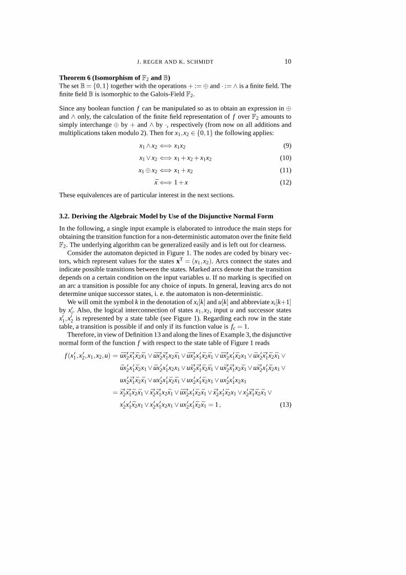
Theorem 6 (Isomorphism ofF2 and B)The setB = {0,1} together with the operations+ := ⊕ and· :=∧ is a finite field. Thefinite field B is isomorphic to the Galois-FieldF2.
Since any boolean functionf can be manipulated so as to obtain an expression in⊕and∧ only, the calculation of the finite field representation off overF2 amounts tosimply interchange⊕ by + and∧ by ·, respectively (from now on all additions andmultiplications taken modulo 2). Then forx1,x2 ∈ {0,1} the following applies:
x1∧x2 ⇐⇒ x1x2 (9)
x1∨x2 ⇐⇒ x1 +x2+x1x2 (10)
x1⊕x2 ⇐⇒ x1 +x2 (11)
x ⇐⇒ 1+x (12)
These equivalences are of particular interest in the next sections.
3.2. Deriving the Algebraic Model by Use of the Disjunctive Normal Form
In the following, a single input example is elaborated to introduce the main steps forobtaining the transition function for a non-deterministicautomaton over the finite fieldF2. The underlying algorithm can be generalized easily and is left out for clearness.
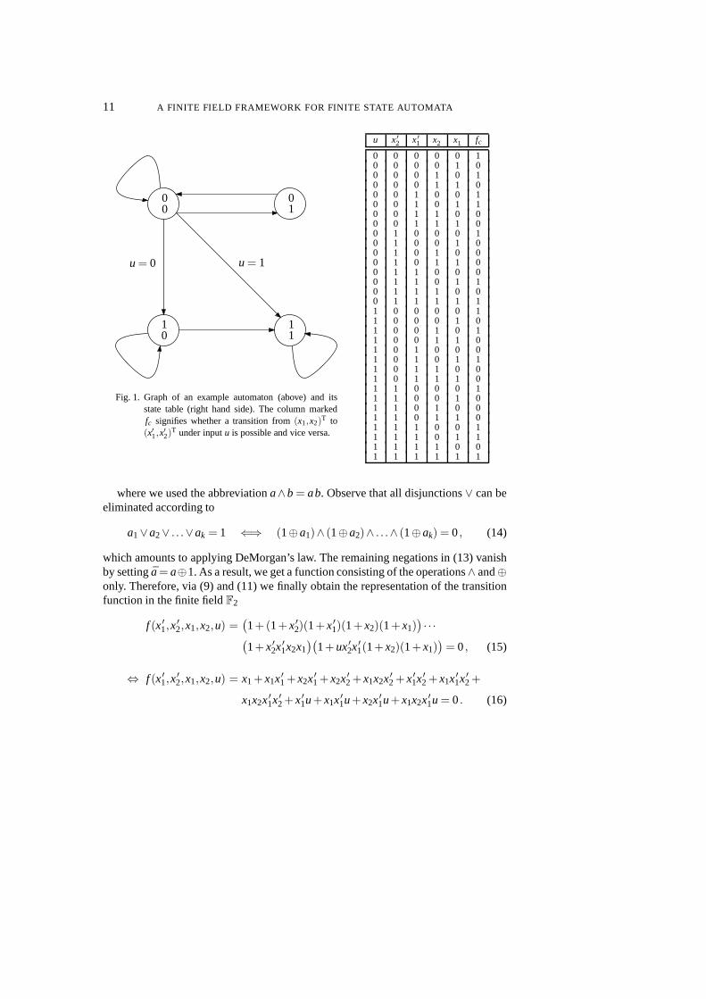
Consider the automaton depicted in Figure 1. The nodes are coded by binary vec-tors, which represent values for the statesxT = (x1,x2). Arcs connect the states andindicate possible transitions between the states. Marked arcs denote that the transitiondepends on a certain condition on the input variablesu. If no marking is specified onan arc a transition is possible for any choice of inputs. In general, leaving arcs do notdetermine unique successor states, i. e. the automaton is non-deterministic.
We will omit the symbolk in the denotation ofxi [k] andu[k] and abbreviatexi [k+1]by x′i . Also, the logical interconnection of statesx1,x2, input u and successor statesx′1,x
′2 is represented by a state table (see Figure 1). Regarding each row in the state
table, a transition is possible if and only if its function value is fc = 1.Therefore, in view of Definition 13 and along the lines of Example 3, the disjunctive
normal form of the functionf with respect to the state table of Figure 1 reads
f (x′1,x′2,x1,x2,u) = ux′2x′1x2x1∨ ux′2x′1x2x1∨ ux′2x′1x2x1∨ ux′2x′1x2x1∨ ux′2x′1x2x1∨
ux′2x′1x2x1∨ ux′2x′1x2x1∨ux′2x′1x2x1∨ux′2x′1x2x1∨ux′2x′1x2x1∨ux′2x′1x2x1∨ux′2x′1x2x1∨ux′2x′1x2x1∨ux′2x′1x2x1
= x′2x′1x2x1∨ x′2x′1x2x1∨ ux′2x′1x2x1∨ x′2x′1x2x1∨x′2x′1x2x1∨x′2x′1x2x1∨x′2x′1x2x1∨ux′2x′1x2x1 = 1, (13)
11 A FINITE FIELD FRAMEWORK FOR FINITE STATE AUTOMATA
00
10
01
11
u = 0 u = 1
Fig. 1. Graph of an example automaton (above) and itsstate table (right hand side). The column markedfc signifies whether a transition from(x1,x2)
T to(x′1,x
′2)
T under inputu is possible and vice versa.
u x′2 x′1 x′2 x′1 fc
0 0 0 0 0 10 0 0 0 1 00 0 0 1 0 10 0 0 1 1 00 0 1 0 0 10 0 1 0 1 10 0 1 1 0 00 0 1 1 1 00 1 0 0 0 10 1 0 0 1 00 1 0 1 0 00 1 0 1 1 00 1 1 0 0 00 1 1 0 1 10 1 1 1 0 00 1 1 1 1 11 0 0 0 0 11 0 0 0 1 01 0 0 1 0 11 0 0 1 1 01 0 1 0 0 01 0 1 0 1 11 0 1 1 0 01 0 1 1 1 01 1 0 0 0 11 1 0 0 1 01 1 0 1 0 01 1 0 1 1 01 1 1 0 0 11 1 1 0 1 11 1 1 1 0 01 1 1 1 1 1
where we used the abbreviationa∧b = ab. Observe that all disjunctions∨ can beeliminated according to
a1∨a2∨ . . .∨ak = 1 ⇐⇒ (1⊕a1)∧ (1⊕a2)∧ . . .∧ (1⊕ak) = 0, (14)
which amounts to applying DeMorgan’s law. The remaining negations in (13) vanishby setting ¯a= a⊕1. As a result, we get a function consisting of the operations∧ and⊕only. Therefore, via (9) and (11) we finally obtain the representation of the transitionfunction in the finite fieldF2
f (x′1,x′2,x1,x2,u) =
(1+(1+x′2)(1+x′1)(1+x2)(1+x1)
)· · ·
(1+x′2x
′1x2x1
)(1+ux′2x
′1(1+x2)(1+x1)
)= 0, (15)
⇔ f (x′1,x′2,x1,x2,u) = x1 +x1x′1 +x2x′1 +x2x′2 +x1x2x′2 +x′1x
′2 +x1x
′1x′2 +
x1x2x′1x′2 +x′1u+x1x′1u+x2x
′1u+x1x2x′1u = 0. (16)

J. REGER AND K. SCHMIDT 12
3.3. Simplifications Using Reed-Muller Generator Matrices
The regular tabulation of the state table in Figure 1 — which is binary counting, rowby row — allows an efficient calculation of the transition function f . So-called Reed-Muller codes, well-known from linear coding theory, are based on this property [8].
Consider the recursively defined Reed-Muller generator matrices
Gi :=
(Gi−1 0Gi−1 Gi−1
)
, G0 := 1 . (17)
Then following [8] we have the simple matrix–vector productoverF2
c2n+m = G2n+mfc , (18)
in which c2n+m is the(22n+m,1)-vector of coefficients associated to a particular tab-ulation of monomials in a(22n+m,1)-vectorϕϕϕ2n+m. In general,ϕϕϕ2n+m contains allmonomials of then statesxi , of them inputsui and of the next statesx′i . The vectorfc is the(22n+m,1)-vector with respect to the rightmost column in the state table ofFigure 1. Using equation (18) the demanded transition function
f (x′1,x′2, . . . ,x
′n,x1,x2, . . . ,xn,u1,u2, . . . ,um) = cT
2n+mϕϕϕT2n+m+1 = 0 (19)
follows. It remains to explain how to tabulate the monomialsin ϕϕϕ2n+m. We return tothe example of Figure 1 withn = 2 states andm= 1 inputs. In this case we have
G5=
1 0 0 0 0 0 0 0 0 0 0 0 0 0 0 0 0 0 0 0 0 0 0 0 0 0 0 0 0 0 0 0
1 1 0 0 0 0 0 0 0 0 0 0 0 0 0 0 0 0 0 0 0 0 0 0 0 0 0 0 0 0 0 0
1 0 1 0 0 0 0 0 0 0 0 0 0 0 0 0 0 0 0 0 0 0 0 0 0 0 0 0 0 0 0 0
1 1 1 1 0 0 0 0 0 0 0 0 0 0 0 0 0 0 0 0 0 0 0 0 0 0 0 0 0 0 0 0
1 0 0 0 1 0 0 0 0 0 0 0 0 0 0 0 0 0 0 0 0 0 0 0 0 0 0 0 0 0 0 0
1 1 0 0 1 1 0 0 0 0 0 0 0 0 0 0 0 0 0 0 0 0 0 0 0 0 0 0 0 0 0 0
1 0 1 0 1 0 1 0 0 0 0 0 0 0 0 0 0 0 0 0 0 0 0 0 0 0 0 0 0 0 0 0
1 1 1 1 1 1 1 1 0 0 0 0 0 0 0 0 0 0 0 0 0 0 0 0 0 0 0 0 0 0 0 0
1 0 0 0 0 0 0 0 1 0 0 0 0 0 0 0 0 0 0 0 0 0 0 0 0 0 0 0 0 0 0 0
1 1 0 0 0 0 0 0 1 1 0 0 0 0 0 0 0 0 0 0 0 0 0 0 0 0 0 0 0 0 0 0
1 0 1 0 0 0 0 0 1 0 1 0 0 0 0 0 0 0 0 0 0 0 0 0 0 0 0 0 0 0 0 0
1 1 1 1 0 0 0 0 1 1 1 1 0 0 0 0 0 0 0 0 0 0 0 0 0 0 0 0 0 0 0 0
1 0 0 0 1 0 0 0 1 0 0 0 1 0 0 0 0 0 0 0 0 0 0 0 0 0 0 0 0 0 0 0
1 1 0 0 1 1 0 0 1 1 0 0 1 1 0 0 0 0 0 0 0 0 0 0 0 0 0 0 0 0 0 0
1 0 1 0 1 0 1 0 1 0 1 0 1 0 1 0 0 0 0 0 0 0 0 0 0 0 0 0 0 0 0 0
1 1 1 1 1 1 1 1 1 1 1 1 1 1 1 1 0 0 0 0 0 0 0 0 0 0 0 0 0 0 0 0
1 0 0 0 0 0 0 0 0 0 0 0 0 0 0 0 1 0 0 0 0 0 0 0 0 0 0 0 0 0 0 0
1 1 0 0 0 0 0 0 0 0 0 0 0 0 0 0 1 1 0 0 0 0 0 0 0 0 0 0 0 0 0 0
1 0 1 0 0 0 0 0 0 0 0 0 0 0 0 0 1 0 1 0 0 0 0 0 0 0 0 0 0 0 0 0
1 1 1 1 0 0 0 0 0 0 0 0 0 0 0 0 1 1 1 1 0 0 0 0 0 0 0 0 0 0 0 0
1 0 0 0 1 0 0 0 0 0 0 0 0 0 0 0 1 0 0 0 1 0 0 0 0 0 0 0 0 0 0 0
1 1 0 0 1 1 0 0 0 0 0 0 0 0 0 0 1 1 0 0 1 1 0 0 0 0 0 0 0 0 0 0
1 0 1 0 1 0 1 0 0 0 0 0 0 0 0 0 1 0 1 0 1 0 1 0 0 0 0 0 0 0 0 0
1 1 1 1 1 1 1 1 0 0 0 0 0 0 0 0 1 1 1 1 1 1 1 1 0 0 0 0 0 0 0 0
1 0 0 0 0 0 0 0 1 0 0 0 0 0 0 0 1 0 0 0 0 0 0 0 1 0 0 0 0 0 0 0
1 1 0 0 0 0 0 0 1 1 0 0 0 0 0 0 1 1 0 0 0 0 0 0 1 1 0 0 0 0 0 0
1 0 1 0 0 0 0 0 1 0 1 0 0 0 0 0 1 0 1 0 0 0 0 0 1 0 1 0 0 0 0 0
1 1 1 1 0 0 0 0 1 1 1 1 0 0 0 0 1 1 1 1 0 0 0 0 1 1 1 1 0 0 0 0
1 0 0 0 1 0 0 0 1 0 0 0 1 0 0 0 1 0 0 0 1 0 0 0 1 0 0 0 1 0 0 0
1 1 0 0 1 1 0 0 1 1 0 0 1 1 0 0 1 1 0 0 1 1 0 0 1 1 0 0 1 1 0 0
1 0 1 0 1 0 1 0 1 0 1 0 1 0 1 0 1 0 1 0 1 0 1 0 1 0 1 0 1 0 1 0
1 1 1 1 1 1 1 1 1 1 1 1 1 1 1 1 1 1 1 1 1 1 1 1 1 1 1 1 1 1 1 1
, ϕϕϕ5=
1
x1x2x1x2x′1x1x′1x2x′1x1x2x′1x′2x1x′2x2x′2x1x2x′2x′1x′2x1x′1x′2x2x′1x′2x1x2x′1x′2u
x1u
x2u
x1x2u
x′1u
x1x′1u
x2x′1u
x1x2x′1u
x′2u
x1x′2u
x2x′2u
x1x2x′2u
x′1x′2u
x1x′1x′2u
x2x′1x′2u
x1x2x′1x′2u
(20)
13 A FINITE FIELD FRAMEWORK FOR FINITE STATE AUTOMATA
with the Reed-Muller generator matrixG5 and the vector of monomialsϕϕϕ5. The tabu-lation regarding the elements ofϕϕϕ5 is carried out recursively: if we start the inspectionwith the vector entry 1 from the top, then for every new variable, the vector is extendedby a copy of the former part of the vector multiplied with the new variable, and so on.Substituting (20) in (18) and (19) verifies the result from (16).
3.4. Enhancements and Generalizations
Abstracting from the latter exemplary viewpoint, in general we obtain a multilineartransition functionf : Fn
2×Fn2×Fm
2 → F2
f (x[k+1],x[k],u[k]) = 0 =
∑S1∈2In
∑S2∈2In
∑S3∈2Im
δS1,S2,S3
(
∏j∈S1
x j [k+1])(
∏l∈S2
xl [k])(
∏m∈S3
um[k])
, (21)
with x ∈ Fn2 and u ∈ Fm
2 , where the setsIn = {1,2, . . . ,n}, Im = {1,2, . . . ,m} areindex sets, 2In denotes the (possibly empty) power set ofIn andδS1,S2,S3 are con-stants inF2. If for fixed x[k] andu[k] we focus onx[k+1], we might observe multiplesuccessorsx[k+1]. Strictly speaking, we then should call (21) not a function,but arelation. As a consequence, the finite field representation (21) is capable of modelingnon-deterministic finite state automata as well.
Leaving aside the details in the following paragraphs, for brevity, we will onlybring to light the ideas of some straight forward extensionsof the setting.
Additional States
Considering more detailed and refined process models often is the remedy againstthe lack of information in coarse automaton models. In this process, usually furtherstates and inputs have to be added to the automaton model. These further states andinputs may be integrated by concatenating the state table onthe left with the respectivecolumns of the new states and inputs (see Figure 1). Using theassociated, bigger Reed-Muller generator matrices, the calculation of the monomialcoefficients in the statetransition function still amounts to the same procedure. However, one special featureof the Reed-Muller approach comes to the fore: only the coefficients referring to thenew variables need to be calculated, the coefficients of the former representation areleft unchanged. This is one major advantage of the Reed-Muller approach.
Partially Defined Transition Functions
A partially defined transition function is a functionf : X ×X ×U → F2 which isdefined on proper subsetsX ⊂ Fn
2 andU ⊂ Fm2 , respectively. This means that only

J. REGER AND K. SCHMIDT 14
some states and inputs may be defined, for example not the whole number of 2n states.Accordingly, only a few rows in the entire state table may be defined. To this accounta check functionr(x1, . . . ,xn,u1, . . . ,um) can be introduced in the same manner asfc.The value ofr equals 0 if the respective state and/or input is defined, and 1elsewhere.Finally, the check functionr and the transition functionf can be combined in onesingle equation. Thus, for a statex[k] and an inputu[k] the extended transition functionis 0 if and only ifx[k] ∈ X andu[k] ∈ U .
Determinism
In case of deterministic automata, the state tables can be reshaped as illustrated inFigure 2. Thus, by employing the methods of Section 3.2 and 3.3 an explicit transitionfunction, a so-called state equation, can be determined. This results in
x[k+1] = f(x[k],u[k]), x ∈ Fn2, u ∈ F
m2 (22)
and reminds of a discrete time system in the continuous world. In the next sections wewill restrict the further examinations to the deterministic linear case.
um · · · u2 u1 x′′
n · · · x2 x1 x′n · · · x′2 x′10 · · · 0 0 0 · · · 0 0 fn,1 · · · f2,1 f1,10 · · · 0 0 0 · · · 0 1 fn,2 · · · f2,2 f1,20 · · · 0 0 0 · · · 1 0 fn,3 · · · f2,3 f1,3... · · ·
......
... · · ·...
...... · · ·
......
1 · · · 1 1 1 · · · 1 1 fn,2n+m · · · f2,2n+m f1,2n+m
Fig. 2. Scheme of a state table for a deterministic automaton
4. ANALYSIS OF AUTONOMOUS LINEAR MODULAR SYSTEMS
The modeling power of the finite field framework shall be examined. To this end, weconsider a deterministic, linear system of the form
x[k+1] = Ax[k]+Bu[k], x ∈ Fn2, u ∈ F
m2 , (23)
a so-calledlinear modular system(LMS).3 The matrixA ∈ Fn×n2 is the dynamics
of the system, the matrixB ∈ Fn×m2 is the input matrix. At first, we examine linear
3Usually LMS are defined overFq for some prime numberq. Here, we will loosely speak of an LMS whenwe assume an LMS with characteristicq = 2, unless it is specified differently.
15 A FINITE FIELD FRAMEWORK FOR FINITE STATE AUTOMATA
systems withB = 0, according to the simplest automaton description in (22), that is
x[k+1] = Ax[k], x ∈ Fn2 . (24)
With regard to these linear systems the analysis for cyclic (periodic) states is carriedout, recalling some results from [6, 13]. The properties of finite fields and polynomialsover finite fields, which have been presented in Section 2, will provide the conceptsnecessary for solving the analysis problem.
4.1. Periodic Nullspace Decomposition of a Companion Matrix
Since a graph of an automaton typically shows cyclic and acyclic behavior the statespace of the respective LMS decomposes into aperiodic and periodic subspaces. It isclear that in the autonomous case any information must be included in the dynamicsA. Thus, we ought to investigateA for information about periodic states which arecharacterized by the following definition.
Definition 14 (Period of a State)A statexτ of an LMS is calledτ-periodic if
xτ ∈ Xτ, Xτ :={
ξξξ ∈ Fn2 |∃τ ∈ N, ξξξ = Aτ ξξξ ∧ ∀ i ∈ N, i < τ, ξξξ 6= A i ξξξ
}
,
in whichXτ is denoting the set ofτ-periodic states.
Regarding the linear system (24) we immediately obtain the relation
(Aτ + I)xτ = 0 (25)
for determining theτ-periodic statesxτ ∈ Fn2. An obvious brute force procedure for
calculating theτ-periodic states would be to solve the linearn-th order system (25) forall xτ,τ = 1,2, . . . ,2n. However, this quickly becomes numerically intractable, evenfor small ordersn. Instead, we propose to benefit from a similarity transform of Ainto its rational canonical formArat. This transform only renumbers the state vectorsand retains the elementary divisor polynomials unchanged,thus, periodicity propertiesare preserved. As a consequence, it is possible to examine the periodic subspacesby the rational canonical form of the dynamics, introduced in equation (5), which isstructurally simpler. Accordingly, by transformingx = Tx we rephrase (25) as per
(Aτ + I)xτ = 0 ⇐⇒ (diag(Cτ1,C
τ2, . . . ,C
τN)+ I) xτ = 0, (26)
which equivalently can be expressed as
(Cτii + I) xτi = 0, i = 1, . . . ,N τ = lcm(τ1,τ2, . . . ,τN) , (27)
in which eachτi ∈ N is minimal,xTτ = (xτ1, xτ2, . . . , xτN) with xτ ∈ F
d12 × . . .×F
dN2 , di
is the dimension ofCi , n= ∑Ni=1di and lcm(.) denotes the least common multiple of its

J. REGER AND K. SCHMIDT 16
arguments. Equation (26) indicates that the state space decomposes intoN subspaceswhich can be examined separately. Note that for nilpotent companion matricesCi thematrixCτi
i + I is non-singular. In this case (27) can hold for the zero vector only, and inconsequence it is sufficient to confine the examination on cyclic companion matricesCi . Moreover, asArat is a rational canonical form it contains companion matriceswith respect to powers of individual irreducible polynomials only, hence, it remains toconsider relation (27) in view of a companion matrixC whose defining (characteristic,minimal) polynomialpC(λ) = cpC(λ) = mpC(λ) can be written as
pC(λ) = (pirr,C(λ))e. (28)
The examination will be organized in four steps:4 firstly, it will be recalled that thekernel of a matrixpC(C) can be decomposed intoe nested linear subspaces the di-mensions of which shall be determined in a second step. With the knowledge aboutthese dimensions, the number of states in the respective subspace is clear and the pe-riod of its states can be be derived. Finally, the superposition of the results for alli = 1, . . . ,N subsystems leads to the main theorem of this section.
The following property follows from the fact that the rank deficiency of singularmatrices strictly increases by its exponent.
Lemma 1 (Nesting Property of Nullspaces)Let pC(λ) = (pirr,C(λ))e ∈ F2[λ], e∈ N, be thed-th degree defining polynomial of acompanion matrixC ∈ F
d×d2 . Assume the basis polynomialpC,irr(λ) to be irreducible
overF2. Then the strict inclusion property (nesting) applies
N0 ⊂N1 ⊂N2 ⊂ . . . ⊂Ne = Fd2 , (29)
where theN j are nullspaces,N0 := {0} andN j := Ker((pirr,C(C)) j
), j = 1, . . . ,e.
By virtue of the non-singularity of cyclic companion matricesC it follows
(pirr,C(C)) j x j = 0 ⇐⇒ C(pirr,C(C)) j x j = 0 ⇐⇒ (pirr,C(C)) j Cx j = 0
for anyx j ∈ Ker((pirr,C(C)) j
), j = 1, . . . ,e, which implies
Lemma 2 (Invariance of the Nullspaces)Let (pirr,C)e ∈ F2[λ] be the defining polynomial of the cyclic companion matrixC ∈ F
d×d2 with pirr,C irreducible. Then thej = 1, . . . ,e nullspaces of the matrices
(pirr,C(C)) j are invariant under the transformationC on anyx j ∈ Ker((pirr,C(C)) j
).
In light of Lemma 2, forj = 1, . . . ,e define the mapC|N j : N j →N j such that
C|N j x j = Cx j , ∀x j ∈ N j (30)
4For brevity, only outlines of the proofs are presented.

17 A FINITE FIELD FRAMEWORK FOR FINITE STATE AUTOMATA
describes the action of the linear transformC on the subspaceN j only. Consequently,
(pirr,C(C|N j ))j x j = (pirr,C(C)) j x j , ∀x j ∈ N j (31)
and asx j lies in the kernel ofN j we have
(pirr,C(C|N j ))j x j = 0, ∀x j ∈N j . (32)
Based on the nesting property, stated in Lemma 1, it can be shown that(pirr,C(λ)) j isnot only an annihilating but the minimal polynomial of the matrix C|N j , i. e.
mpC|N j(λ) = (pirr,C(λ)) j . (33)
Since to any minimal polynomial corresponds a companion matrix the dimension ofwhich is the degree of its minimal polynomial, we conclude
Lemma 3 (Dimension of the Nullspaces)Let (pirr,C)e ∈ F2[λ] be the defining polynomial of the cyclic companion matrixC ∈ F
d×d2 with pirr,C irreducible andδ = deg(pirr,C). Let the nullspacesN j :=
Ker((pirr,C(C)) j
), j = 1, . . . ,e. Then the dimension of each nullspaceN j is
dim(N j) = deg((pirr,C) j)= δ j . (34)
It remains to investigate the periods of the subspace states. To this end, lettκ, κ ∈ N,denote the period of the polynomial(pirr,C(λ))κ, hence
g(λ)(pirr,C(λ))κ = λtκ −1 (35)
for some polynomialg(λ) and therefore
g(C|N j )(pirr,C(C|N j ))κ = (C|N j )
tκ − I . (36)
Right-multiplication by an arbitrary statex j ∈ N j yields
g(C|N j )(pirr,C(C|N j ))κ x j = ((C|N j )
tκ − I)x j . (37)
Thusx j is tκ-periodic if
(pirr,C(C|N j ))κ x j = 0, (38)
which is the case ifx j ∈ Nκ. DefiningD j := N j\N j−1, j = 1, . . . ,e, the states inDκturn out to be exactly those which areτκ-periodic, and we obtain
Lemma 4 (Period of the States inD j )Let the dynamics matrix of an LMS be given by a cyclic companion matrixC ∈ F
d×d2
the defining polynomial(pirr,C)e ∈ F2[λ] of which is the power of an irreducible poly-nomial pirr,C. Furthermore, letD j := N j\N j−1, j = 1, . . . ,e. Then any state vector inthe setD j is τ j -periodic, whereτ j is the period of the polynomial(pirr,C(λ)) j .

J. REGER AND K. SCHMIDT 18
Recalling δ = deg(pirr,C), all q jδ − q( j−1)δ states inD j have periodτ j such thatν j =
(q jδ − q( j−1)δ)/τ j cycles ofτ j -periodic states lie in the spaceD j . Adding up
the number of states inD j from j = 1, . . . ,e plus the remaining zero state results in
1+e
∑j=1
q jδ −q( j−1)δ = qeδ = qd (39)
which shows that the entire spaceFd2 is composed of these cycles. Collecting all lem-
mas and referring to Theorem 3 for the period of powered polynomials implies
Theorem 7 (Periodic Nullspace Decomposition of a CompanionMatrix)Given a cyclic companion matrixC∈F
d×d2 with respect to thed-th degree polynomial
pC = (pirr,C)e, wherepirr,C ∈ F2[λ] is irreducible with degreeδ such thatd = eδ. Thenthe associated state spaceFd
2 is entirely composed of periodic states as per
ν0 = 1 cycles of length τ0 = 1ν1 =
(2δ −1
)/τ1 ” τ1 = τ
ν2 =(22δ −2δ)/τ2 ” τ2 = 2τ
. . . . . . . . . . . . . . . . . . . . . . . . . . . . . . . . . . . . . . . . . . . . . . . . . . .. . . . .ν j =
(2 jδ −2( j−1)δ)/τ j ” τ j = 2l j τ
. . . . . . . . . . . . . . . . . . . . . . . . . . . . . . . . . . . . . . . . . . . . . . . . . . .. . . . .νe =
(2eδ −2(e−1)δ)/τe ” τe = 2le τ
where eachl j , j = 1, . . . ,e, is the least integer such that 2l j ≥ j.
The periodic decomposition can be written in a more convenient form by applying
Definition 15 (Cycle Sum)The cycle sumΣ is the formal sum of cycle terms
Σ = ν1[τ1]u ν2[τ2]u . . .u νκ[τNΣ ] , (40)
in which the cycle termνi [τi ] denotesνi cycles of lengthτi and the binary operationu satisfiesνi [τ]u ν j [τ] = (νi + ν j)[τ]. The number of cycles inΣ is denoted byNΣ.
Using this definition the result of Theorem 7 can be rewrittenas
Σ = 1[1]u2δ −1
τ1[τ1]u
22δ −2δ
τ2[τ2]u . . .u
2eδ −2(e−1)δ
τe[τe] , (41)
in which τ j , j = 1, . . . ,e, marks the periods of the polynomial(pirr,C(λ)) j which canbe computed via Theorem 3.
19 A FINITE FIELD FRAMEWORK FOR FINITE STATE AUTOMATA
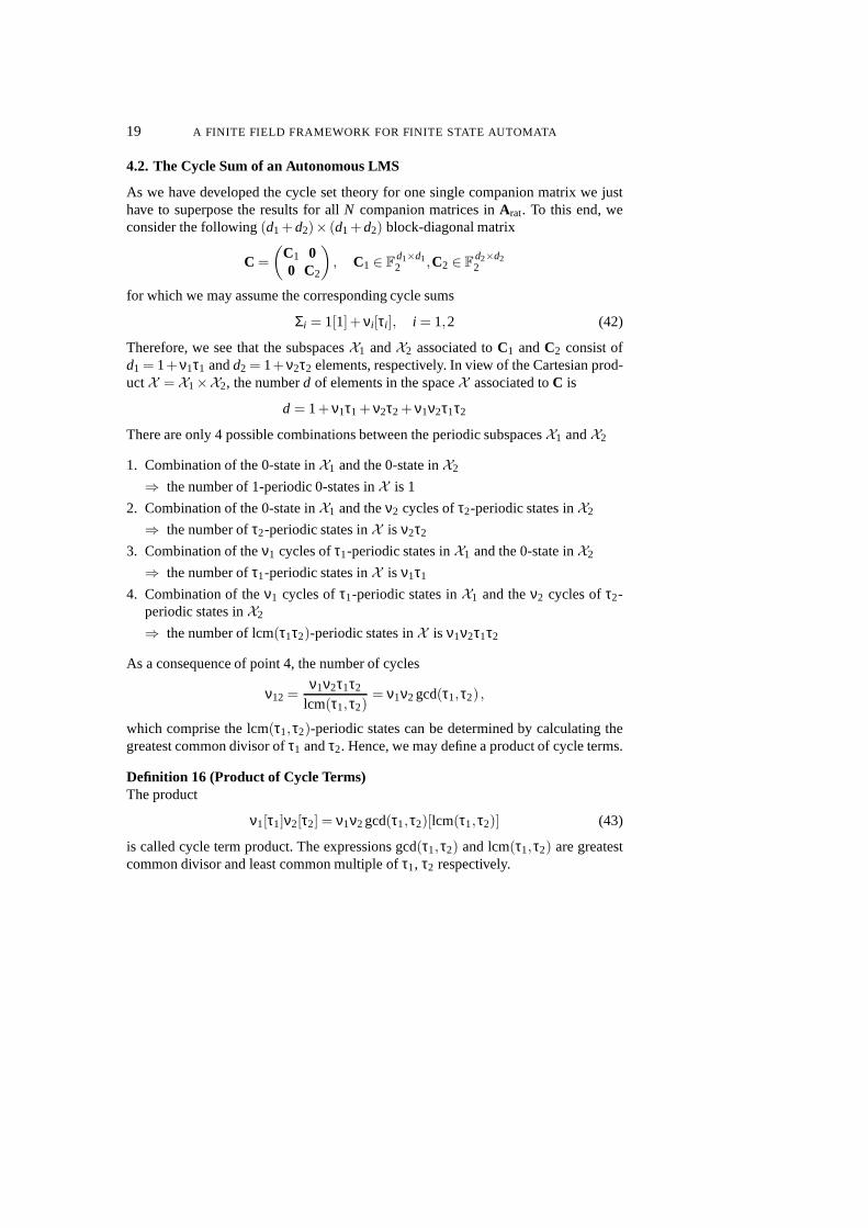
4.2. The Cycle Sum of an Autonomous LMS
As we have developed the cycle set theory for one single companion matrix we justhave to superpose the results for allN companion matrices inArat. To this end, weconsider the following(d1 +d2)× (d1+d2) block-diagonal matrix
C =
(C1 00 C2
)
, C1 ∈ Fd1×d12 ,C2 ∈ F
d2×d22
for which we may assume the corresponding cycle sums
Σi = 1[1]+ νi[τi ], i = 1,2 (42)
Therefore, we see that the subspacesX1 andX2 associated toC1 andC2 consist ofd1 = 1+ν1τ1 andd2 = 1+ν2τ2 elements, respectively. In view of the Cartesian prod-uctX = X1×X2, the numberd of elements in the spaceX associated toC is
d = 1+ ν1τ1 + ν2τ2 + ν1ν2τ1τ2
There are only 4 possible combinations between the periodicsubspacesX1 andX2
1. Combination of the 0-state inX1 and the 0-state inX2
⇒ the number of 1-periodic 0-states inX is 1
2. Combination of the 0-state inX1 and theν2 cycles ofτ2-periodic states inX2
⇒ the number ofτ2-periodic states inX is ν2τ2
3. Combination of theν1 cycles ofτ1-periodic states inX1 and the 0-state inX2
⇒ the number ofτ1-periodic states inX is ν1τ1
4. Combination of theν1 cycles ofτ1-periodic states inX1 and theν2 cycles ofτ2-periodic states inX2
⇒ the number of lcm(τ1τ2)-periodic states inX is ν1ν2τ1τ2
As a consequence of point 4, the number of cycles
ν12 =ν1ν2τ1τ2
lcm(τ1,τ2)= ν1ν2 gcd(τ1,τ2) ,
which comprise the lcm(τ1,τ2)-periodic states can be determined by calculating thegreatest common divisor ofτ1 andτ2. Hence, we may define a product of cycle terms.
Definition 16 (Product of Cycle Terms)The product
ν1[τ1]ν2[τ2] = ν1ν2gcd(τ1,τ2)[lcm(τ1,τ2)] (43)
is called cycle term product. The expressions gcd(τ1,τ2) and lcm(τ1,τ2) are greatestcommon divisor and least common multiple ofτ1, τ2 respectively.

J. REGER AND K. SCHMIDT 20
By means of the denotation of sum and product of cycle terms, from (42) we extendthe notion of product to the superpositionΣ of the cycle sumsΣ1 andΣ2
Σ = Σ1Σ2 = (1[1]u ν1[1])(1[1]u ν2[2]) =
1[1]u ν1[τ1]u ν2[τ2]u ν1ν2gcd(τ1,τ2)[lcm(τ1,τ2)] (44)
The next theorem is an obvious generalization of the latter.
Theorem 8 (Superposition)The cycle sumΣ superposingN cycle sumsΣi , i = 1, . . . ,N can be calculated distribu-tively by the product
Σ = Σ1Σ2 · · ·ΣN . (45)
All together we finally have shown
Theorem 9 (Cycle Sum of an Autonomous LMS)Let the dynamicsA = diag(C1, . . . ,CN) ∈ F
n×n2 of an autonomous LMS(q) be block
diagonally composed ofi = 1, . . . ,N cyclic companion matricesCi , each with respectto one of thei = 1, . . . ,N elementary divisor polynomialspCi ∈ F2[λ] of degreedi .Let each elementary divisor polynomialpCi be given in fully factorized formpCi =(pirr,Ci )
ei subject to its irreducible factor polynomialpirr,Ci of degreeδi such thatdi =ei δi . Then each elementary divisor polynomialpCi contributes the cycle sum
Σi = 1[1]u2δi −1
τ(i)1
[τ(i)
1
]u
22δi −2δi
τ(i)2
[τ(i)
2
]u . . .u
2eiδi −2(ei−1)δi
τ(i)ei
[τ(i)
ei
], (46)
whereτ(i)j denotes the period5 of the polynomial(pirr,Ci )
j . The cycle sumΣ of the au-tonomous LMS follows from Superposition of all cycle sumsΣi as perΣ = Σ1Σ2 · · ·ΣN.
Remark 4As already pointed out in Remark 1, a simple consequence of Theorem 9 is that nilpo-tent elementary divisor polynomials are not related to periodic subspaces.
Subsumingly, the whole cycle sum of a linear modular system over F2 can be calcu-lated along the following algorithm:
1. Calculate the Smith normal formS(λ) of A by unimodular left and right trans-forms onλI + A via polynomial matricesU(λ) andV(λ) (alternatively calculatethe rational canonical formArat of A).
5At least here we are justified to have introduced the same symbol τ for the period of a state although firstlyτ was introduced for the period of polynomials in Definition 7.

21 A FINITE FIELD FRAMEWORK FOR FINITE STATE AUTOMATA
2. Determine theN elementary divisor polynomialspi(λ), i = 1, . . . ,N of A by fac-torizing the system invariants inS(λ).
3. Assign the periodsτ(i)j to each polynomialp j
i,irr(λ), j = 1, . . . ,ei with pi(λ) =
peii,irr(λ) andpi,irr(0) 6= 0 (due to Remark 4 we omit polynomialspi(λ) = λk,k∈N).
4. Compute the cycle sumΣi for each elementary divisor polynomialpi(λ).
5. The cycle sumΣ of the entire automaton then follows by distributively superposingall cycle setsΣi , i = 1, . . . ,N.
4.3. Example
Consider the dynamics matrixA ∈ F5×52 of an LMS with its respective Smith form
S(λ) = U(λ)(λI +A)V(λ) according to
A =
1 0 0 1 11 1 0 0 10 0 1 0 10 0 0 0 11 0 0 0 1
, S(λ) =
(λ2 + λ +1)(λ +1)2 0 0 0 00 λ +1 0 0 00 0 1 0 00 0 0 1 00 0 0 0 1
.
Then the only invariant polynomials of the matrixA which are different from 1 are
c1(λ) = (λ2 + λ +1)(λ +1)2, c2(λ) = λ +1 .
Hence,A has the elementary divisor polynomials
p1(λ) = λ2 + λ +1, p2(λ) = (λ +1)2, p3(λ) = λ +1 ,
the irreducible basis polynomial degrees of which areδ1 = 2, δ2 = 1 andδ3 = 1, re-spectively. In view of Definition 7 and Theorem 3 we calculatethe associated periods:
p1,irr(λ) = p1(λ)|λ3 +1 =⇒ τ(1)1 =3
p2,irr(λ) = λ +1 =⇒ τ(2)1 =1
(p2,irr(λ)
)2= (λ +1)2 = λ2 +1 =⇒ τ(2)
2 =2
p3,irr(λ) = λ +1 =⇒ τ(3)1 =1
Theorem 9 yields
Σ1 = 1[1]u1[3], Σ2 = 2[1]u1[2], Σ3 = 2[1]
and by superposition according to Theorem 8 and using (15) and (43), we get
Σ = Σ1Σ2Σ3 = (1[1]u1[3])(2[1]u1[2])(2[1])=
(2[1]u1[2]u2[3]u1[6])(2[1])= 4[1]u2[2]u4[3]u2[6] .

J. REGER AND K. SCHMIDT 22
Therefore, the considered linear automaton given by the dynamicsA comprises 4cycles of length 1, 2 cycles of length 2, 4 cycles of length 3 and 2 cycles of length 6.
5. PROPERTIES OF LINEAR MODULAR SYSTEMS WITH INPUTS
As the main goal of this paper involves the synthesis of a control for linear discretesystems overF2 the notion of controllability of an LMS has to be taken into account.For this purpose the well-known solution
x[k] = Ak x[0]+k−1
∑i=0
Ak−1−i Bu[i]. (47)
of the state equation (23) of an LMS is recalled from [2]. Owing to this result, con-trollability can be defined for an LMS and a controllability criterion can be specified.
Definition 17 (Controllability)An n-th order LMS isl -controllable iff for all ordered pairs of states(x1,x2) the systemcan be driven from statex1 to statex2 in exactlyl steps. An LMS is controllable iff itis l -controllable for somel .
Theorem 10 (Controllability Criterion)An n-th order LMS isl -controllable iff the matrix(B AB . . . A l−1B) has full rankn.
This theorem will be used for establishing the controllability companion form, whichcan be determined by applying linear transforms on the stateequation.
Using Theorem 10 the reduced controllability matrixL ∈ Fn×n2 of an LMS can be
determined by choosingn linearly independent columns from(B AB . . . A l−1B) withregard to minimal multiples ofA, see [17]. This procedure yields the matrix
L =(b1. . .Ac1−1b1 b2. . .Ac2−1b2 . . . bm . . . Acm−1bm
), (48)
where the vectorsbi , i = 1, . . . ,m, are the respective column vectors of the input matrixB and the numbersci ∈ N are the controllability indices with the properties:
r the set ofci is unique,r the set ofci is invariant with respect to similarity transformations,r ∑m
i=1ci = n,r the listσi := ∑i
j=1c j , i = 1, . . . ,m, implies a structural system decomposition.
Given a controllable LMS, a characteristic companion form of the state equations (23)can be found using a similarity transformation which employs (48) and the set ofcontrollability indicesci [17]. It is called the controllability companion form (CCF),
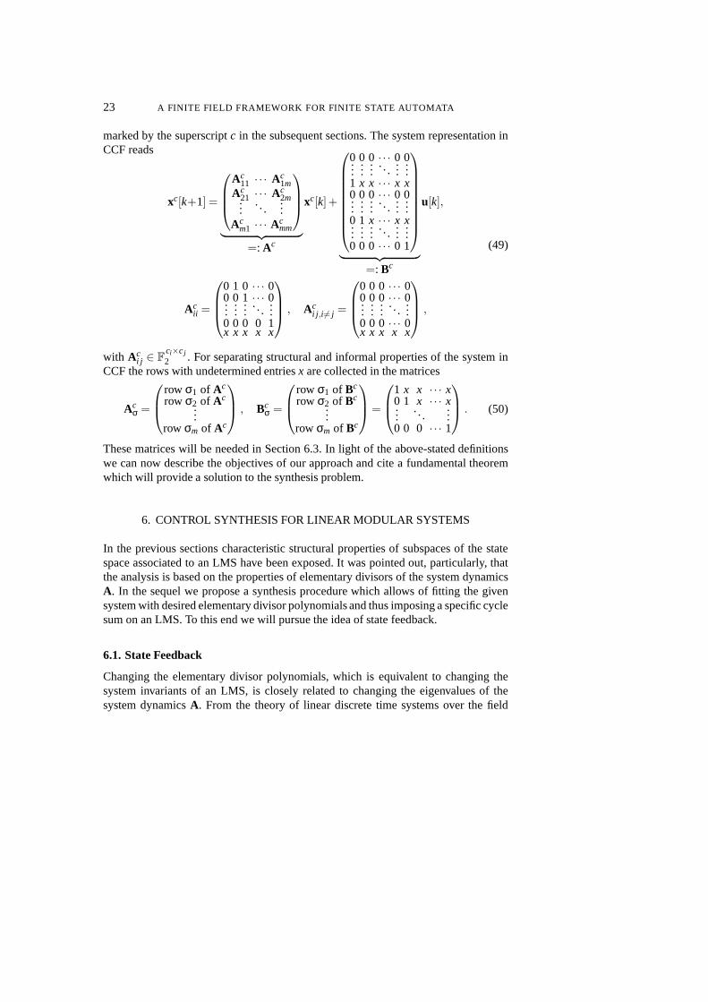
23 A FINITE FIELD FRAMEWORK FOR FINITE STATE AUTOMATA
marked by the superscriptc in the subsequent sections. The system representation inCCF reads
xc[k+1] =
Ac11 · · · Ac
1mAc
21 · · · Ac2m...
. . ....
Acm1 · · · Ac
mm
︸ ︷︷ ︸
=: Ac
xc[k]+
0 0 0 · · · 0 0......
.... . .
......
1 x x · · · x x0 0 0 · · · 0 0...
......
. . ....
...0 1 x · · · x x...
......
. . ....
...0 0 0 · · · 0 1
︸ ︷︷ ︸
=: Bc
u[k],
Acii =
0 1 0 · · · 00 0 1 · · · 0...
......
. . ....
0 0 0 0 1x x x x x
, Aci j ,i6= j =
0 0 0 · · · 00 0 0 · · · 0...
......
. . ....
0 0 0 · · · 0x x x x x
,
(49)
with Aci j ∈ F
ci×cj2 . For separating structural and informal properties of the system in
CCF the rows with undetermined entriesx are collected in the matrices
Acσ =
row σ1 of Ac
row σ2 of Ac...
row σm of Ac
, Bc
σ =
row σ1 of Bc
row σ2 of Bc...
row σm of Bc
=
1 x x · · · x0 1 x · · · x...
. . ....
0 0 0 · · · 1
. (50)
These matrices will be needed in Section 6.3. In light of the above-stated definitionswe can now describe the objectives of our approach and cite a fundamental theoremwhich will provide a solution to the synthesis problem.
6. CONTROL SYNTHESIS FOR LINEAR MODULAR SYSTEMS
In the previous sections characteristic structural properties of subspaces of the statespace associated to an LMS have been exposed. It was pointed out, particularly, thatthe analysis is based on the properties of elementary divisors of the system dynamicsA. In the sequel we propose a synthesis procedure which allowsof fitting the givensystem with desired elementary divisor polynomials and thus imposing a specific cyclesum on an LMS. To this end we will pursue the idea of state feedback.
6.1. State Feedback
Changing the elementary divisor polynomials, which is equivalent to changing thesystem invariants of an LMS, is closely related to changing the eigenvalues of thesystem dynamicsA. From the theory of linear discrete time systems over the field
J. REGER AND K. SCHMIDT 24
of real numbersR it is well-known that changing the eigenvalues ofA can be doneby introducing a (static) linear state feedback of the formu[k] = −Kx [k]+w[k] withthe constant feedback matrixK ∈ F
m×n2 and the reference input vectorw[k] ∈ Fm
2 .Referring to this concept it is intuitive to introduce a linear state feedback
u[k] = Kx [k]+w[k] (51)
for the control of an LMS as well. This leeds to the closed-loop state representation
x[k+1] = (A +BK)x[k]+Bw[k]. (52)
The invariants of the dynamicsA +BK can be specified by the state feedbackK .
6.2. Structural Constraints
The closed-loop system (52) complies with the structure theorem, recalled from [9].
Theorem 11 (Rosenbrock Structure Theorem)Given ann-th order controllable LMS with controllability indicesc1 ≥ . . . ≥ cm anddesired monic invariant polynomialsci,K ∈ F2[λ] with deg(c1,K ) ≥ . . . ≥ deg(cm,K ),ci+1,K |ci,K , i = 1, . . . ,m− 1, and∑m
i=1deg(ci,K ) = n. Then a constant matrixK suchthatA +BK has the invariant polynomialsci,K exists iff fork = 1,2, . . . ,m
k
∑i=1
deg(ci,K ) ≥k
∑i=1
ci . (53)
Rosenbrock’s structure theorem entails a limit when striving for maximal liberalityin specifying invariant polynomials. There are many methods for computing a linearstate feedback, mainly by specifying desired eigenvalues in some “time domain”.
Intuitively, pole placing methods seem to be applicable. But specifying invari-ant polynomials is a stronger requirement than specifying eigenvalues. Consequently,standard pole placing methods can be ruled out. An approach which enables the mod-ification of the eigenstructure of a system is the parametricapproach [15]. However,this approach is not capable of serving the requirements forthe subsequent reasons.
Remark 5Synthesis of state feedback via the parametric approach hasconsiderable drawbacks:
r An assumption in this approach is that the open-loop and the closed-loop eigenval-ues are distinct, which is a very restrictive assumption in the framework of LMS.
r Assigning multiple eigenvalues, which is indispensable for the realization of ratherstandard cycle sums (e. g. cycles of even length), turns out to be very cumbersomeas the computation of generalized eigenvectors is required.
25 A FINITE FIELD FRAMEWORK FOR FINITE STATE AUTOMATA
r As eigenvalues of matrices over a finite fieldFq are roots of a polynomial over afinite field the notion of zeroes is important. These zeroes typically lie in some ex-tension fieldFq that deeply depends on the factors and the degree of the polynomialitself. Moreover, these extension fields have no unique defining element [12]. Thisis a severe difference to the field of real numbers in which anypolynomial inR[λ]can be factorized into quadratic irreducible polynomials overR (see Definition 6).Hence, any zero of a polynomial inR[λ] lies in the corresponding extension field,which is the field of complex numbersC with unique defining elementi =
√−1. In
general, such a factorization is not possible for polynomials in Fq[λ]. Consequently,the computation of eigenvalues in the extension field ofF2 entails enormous sym-bolical computation effort.
r The structural theorem imposes constraints on realizable invariant polynomials inthe closed-loop system. Thus, if the task is to assign invariant polynomials this ismuch more straight-forward in the frequency domain even forcontinuous systems.
In view of these issues we will define an image domain for LMS inthe next section.
6.3. An Image Domain for LMS
Similar to discrete continuous time systems an image domaincan be defined [14].
TheA-Transform
Definition 18 (AAA-Transform)TheA-transform for a causal, discrete functionf : N → F2 is
F(a) := A( f [k]) :=∞
∑k=0
f [k]a−k . (54)
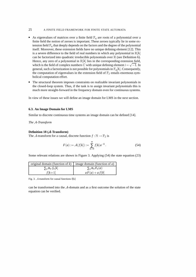
Some relevant relations are shown in Figure 3. Applying (54)the state equation (23)
original domain (function ofk) image domain (function ofa)∑ν αν fν[k] ∑ν αν Fν(a)
f [k+1] aF(a)+a f [0]
Fig. 3. A-transform for causal functions f[k]
can be transformed into theA-domain and as a first outcome the solution of the stateequation can be verified.
J. REGER AND K. SCHMIDT 26
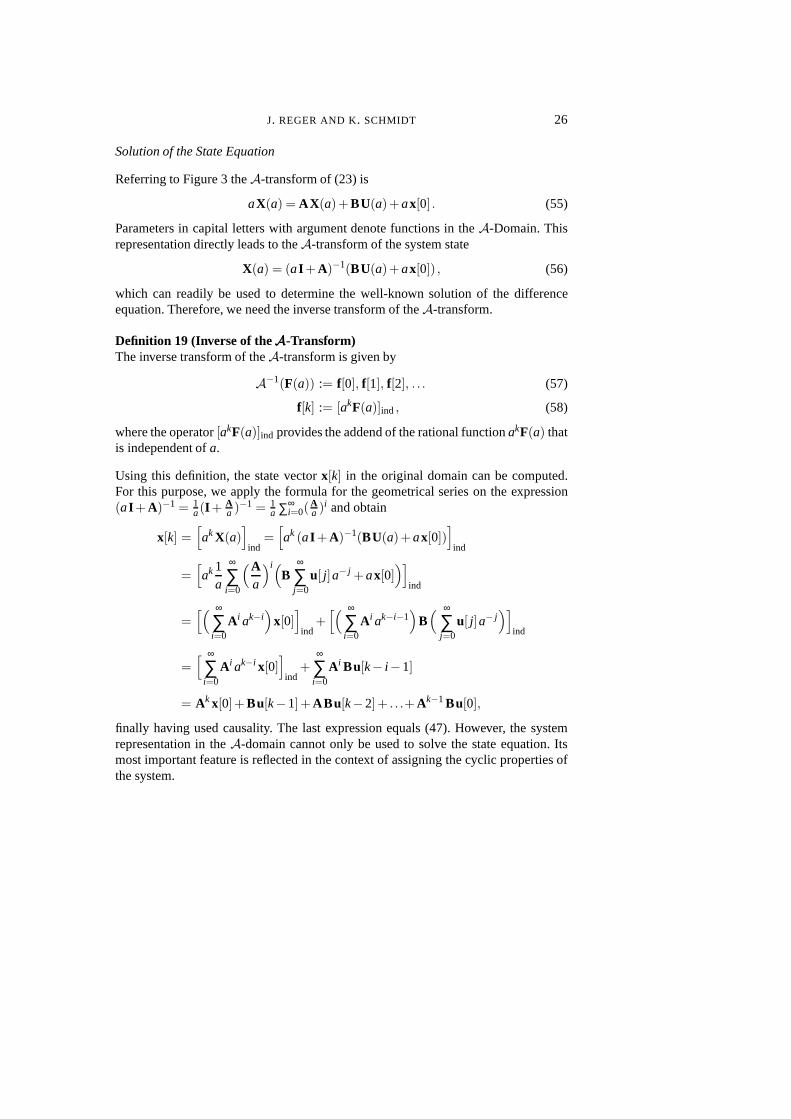
Solution of the State Equation
Referring to Figure 3 theA-transform of (23) is
aX(a) = AX(a)+BU(a)+ax[0] . (55)
Parameters in capital letters with argument denote functions in theA-Domain. Thisrepresentation directly leads to theA-transform of the system state
X(a) = (aI +A)−1(BU(a)+ax[0]) , (56)
which can readily be used to determine the well-known solution of the differenceequation. Therefore, we need the inverse transform of theA-transform.
Definition 19 (Inverse of theAAA-Transform)The inverse transform of theA-transform is given by
A−1(F(a)) := f[0], f[1], f[2], . . . (57)
f[k] := [akF(a)]ind , (58)
where the operator[akF(a)]ind provides the addend of the rational functionakF(a) thatis independent ofa.
Using this definition, the state vectorx[k] in the original domain can be computed.For this purpose, we apply the formula for the geometrical series on the expression(aI +A)−1 = 1
a(I + Aa )−1 = 1
a ∑∞i=0(
Aa )i and obtain
x[k] =[
ak X(a)]
ind=[
ak (aI +A)−1(BU(a)+ax[0])]
ind
=[
ak 1a
∞
∑i=0
(Aa
)i(
B∞
∑j=0
u[ j]a− j +ax[0])]
ind
=[( ∞
∑i=0
A i ak−i)
x[0]]
ind+[( ∞
∑i=0
A i ak−i−1)
B( ∞
∑j=0
u[ j]a− j)]
ind
=[ ∞
∑i=0
A i ak−i x[0]]
ind+
∞
∑i=0
A i Bu[k− i −1]
= Ak x[0]+Bu[k−1]+ABu[k−2]+ . . .+Ak−1Bu[0],
finally having used causality. The last expression equals (47). However, the systemrepresentation in theA-domain cannot only be used to solve the state equation. Itsmost important feature is reflected in the context of assigning the cyclic properties ofthe system.
27 A FINITE FIELD FRAMEWORK FOR FINITE STATE AUTOMATA
Transfer Matrix
In view of (56) we can defineF(a) in
X(a)∣∣∣x[0]=0
= F(a)U(a) = (aI +A)−1BU(a) . (59)
as the system transfer matrix. It is obvious that the cyclic properties of the systemare contained inF(a) as the properties of a periodic system state are described bytheexpression(aI +A), or by(aI +A)−1, alternatively. In the next sections we will com-pute a linear state feedback using (59) by employing the polynomial matrix approach.
Polynomial Matrix Fraction of the Transfer Matrix
For a better understanding, the most important notions and concepts which evolve inthe polynomial matrix approach have to be recalled [17, 11].
Definition 20 (Polynomial Matrix Fraction)A right (left) polynomial matrix fraction RPMF (LPMF) of a rational matrixR(a) isan expression of the following form
R(a) = N(a)D−1(a)(R(a) = D−1(a)N(a)
)(60)
with the polynomial matrices denominator matrixD(a) and numerator matrixN(a).
By means of this definition the following theorem can be stated.
Theorem 12 (Conservation)The product of an arbitrary polynomial matrixR(a) and an arbitrary unimodular poly-nomial matrixU(a) has the same invariant polynomials asR(a).
Due to the fact that the transfer matrix in (59) is a rational matrix, known results onrational matrices can be utilized.
Theorem 13 (Existence)For any rational matrix thereR(a) exists a right (left)-prime polynomial matrix frac-tion representation.
Theorem 14 (Invariant Polynomials)Let R(a) be a rational matrix. Then
r the numerator matrices of arbitrary right- or left-prime polynomial matrix fractionsof R(a) have the same invariant polynomials and
r the denominator matrices of arbitrary right- or left-primepolynomial matrix frac-tions ofR(a) have the same invariant polynomials.
J. REGER AND K. SCHMIDT 28
As the transfer matrix representation in (59) is a left-prime polynomial matrix fraction,Theorem 14 reveals that the invariant polynomials of the denominator matrix of eachpolynomial matrix fraction ofF(a) are equal to the invariant polynomials of the systemdynamicsA. For a system in CCF (see equations (49) and (50)) an analyticexpressionfor a right-prime polynomial matrix fraction can be determined as [17]
F(a) = Q(a)(
(Bcσ)−1(γγγ(a)+Ac
σ Q(a)))−1
, (61)
where the matricesQ(a) andγγγ(a) show the structure
Q(a) =
1 0 · · · 0a 0 · · · 0...
..... .
...ac1−1 0 · · · 0
0 1 · · · 0......
.. ....
0 ac2−1 · · · 0......
.. ....
0 0 · · · 1......
.. ....
0 0 · · · acm−1
, γγγ(a) =
ac1 0 · · · 00 ac2 · · · 0...
..... .
...0 0 · · · acm
. (62)
This means that if the LMS is given in CCF, it is straight-forward to find an expressionfor the polynomial matrix fraction of the system transfer matrix (59). Similarly, for theclosed-system (52) we have the RPMF
F(a) = Q(a)(
(Bcσ)−1(γγγ(a)+
Acσ,K
︷ ︸︸ ︷
(Acσ +Bc
σ K c) Q(a))︸ ︷︷ ︸
DK (a)
)−1(63)
with the following properties:
r The numerator matrixQ(a) of the RPMF is left unchanged by linear state feedback.r The denominator matrixDK (a) and the corresponding closed-loop system dynam-
icsA +BK have the same invariant polynomials.r The controllability indices equal the column degrees6 of the denominator matrix.
Since the feedback matrixK can be uniquely determined ifDK (a) in (63) is known,finding an adequate state feedback for fitting a closed-loop LMS with desired invariantpolynomials amounts to determine a denominator matrixDK (a) with the properties:
1. The invariant polynomials ofDK (a) coincide with the desired polynomialsci,K (a).
6This is the highest polynomial degree in the corresponding column.

29 A FINITE FIELD FRAMEWORK FOR FINITE STATE AUTOMATA
2. The column degrees ofDK (a) equal the controllability indicesci of the LMS.7
With DK (a) = (Bcσ)−1D∗
K (a) it suffices to considerD∗K (a) as(Bc
σ)−1 is unimodularand, thus by Theorem 12,D∗
K (a) has the same invariant polynomials asDK (a).
6.4. Main Theorem
With the results from the previous sections the main theoremfor the synthesis of alinear state feedback can be stated.
Theorem 15 (Synthesis Algorithm)Let a controllable LMS be given in CCF, letci , i = 1, . . . ,m be its controllability in-dices, letci,K ∈ F2[a], i = 1, . . . ,m, be desired invariant polynomials and letD∗(a) =diag(ci,K (a)), i = 1, . . . ,m with deg(c1,K ) ≥ . . . ≥ deg(cm,K ) and ∑m
i=1deg(ci,K ) =
∑mi=1ci = n. The following algorithm is given:8
1. Check the structural theorem forci andci,K (a). If (53) is fulfilled go tostep 2, elsesuch a state feedback matrixK does not exist.
2. ExamineD∗(a).
– if the column degrees ofD∗(a) equal the ordered list of controllability indicesgo tostep 5.
– else detect the first column ofD∗(a) which differs from the ordered listof controllability indices, starting with column 1. Denotethis columncolu.(deg(colu) > cu).
– Do the same beginning with columnm. Denote the specified columncold.(deg(cold) < cd).
3. Adapt the column degrees ofD∗(a) by unimodular transformations.
– Multiply rowd with a and add the result torowu ⇒ D∗(a) → D+(a) .
– if deg(col+u ) = deg(colu)−1
– D+(a) → D++(a) andgo tostep 4.
– else
– define:r := deg(colu)−deg(cold)−1
– multiply col+u with ar and subtract the result fromcol+d .⇒D+(a)→D++(a)
7Controllability indicesci do not change by linear state feedback.8For abbreviation, thei-th matrix columns and rows are denoted bycoli androwi , i = 1, . . . ,m, respectively.

J. REGER AND K. SCHMIDT 30
4. Generate the column pointer matrix9 ΓΓΓ++ of D++(a) ⇒ D∗(a) = (ΓΓΓ++)−1 ·D++(a) andgo tostep 2
5. D∗K (a) := D∗(a) andreturn D ∗
K (a)
If the conditions from above are fulfilled, andD∗K (a) is returned by the algorithm, then
D∗K (a) can be generated by linear state feedbackK .
In Section 6.3 we stated that ifDK (a) is known then it is straightforward to computethe state feedback matrixK . To illustrate this, consider
DK (a) = (Bcσ)−1D∗
K (a)
= (Bcσ)−1(γγγ(a)+Ac
σ,KQ(a))
which leads to
Acσ,KQ(a) = γγγ(a)+Bc
σ DK (a) (64)
and by comparison of coefficients the matrix
Acσ,K = Ac
σ +Bcσ K c (65)
can be determined, which directly providesK c = (Bcσ)−1(Ac
σ,K +Acσ) and thus a feed-
back matrixK c has been derived which fits the given LMS with the desired closed-loop invariant polynomialsci,K , i = 1, . . . ,m. Note that, in general, the solution forD∗
K (a) is not unique.
6.5. Example
In this section we want to illustrate the latter notions by the following state equations
x[k+1] =
0 1 0 0 00 0 1 0 00 0 0 0 00 0 0 0 11 0 0 1 0
x[k]+
0 00 01 00 00 1
u[k] .
9The column pointer matrix is a matrix with elements inF2 consisting of the coefficients of the greatestdegree monomials in each column ofD++(a).
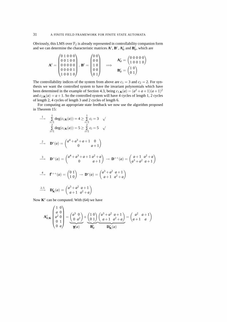
31 A FINITE FIELD FRAMEWORK FOR FINITE STATE AUTOMATA
Obviously, this LMS overF2 is already represented in controllability companion formand we can determine the characteristic matricesAc, Bc, Ac
σ andBcσ, which are
Ac =
0 1 0 0 00 0 1 0 00 0 0 0 00 0 0 0 11 0 0 1 0
, Bc =
0 00 01 00 00 1
=⇒Ac
σ =
(0 0 0 0 01 0 0 1 0
)
Bcσ =
(1 00 1
)
The controllability indices of the system from above arec1 = 3 andc2 = 2. For syn-thesis we want the controlled system to have the invariant polynomials which havebeen determined in the example of Section 4.3, beingc1,K (a) = (a2 +a+1)(a+1)2
andc2,K (a) = a+1. So the controlled system will have 4 cycles of length 1, 2 cyclesof length 2, 4 cycles of length 3 and 2 cycles of length 6.
For computing an appropriate state feedback we now use the algorithm proposedin Theorem 15:
1−→1∑
i=1deg(ci,K (a)) = 4≥
1∑
i=1ci = 3
√
2∑
i=1deg(ci,K (a)) = 5≥
2∑
i=1ci = 5
√
2−→ D∗(a) =
(a4 +a3+a+1 0
0 a+1
)
3−→ D+(a) =
(a4 +a3+a+1 a2 +a
0 a+1
)
→ D++(a) =
(a+1 a2+a
a3 +a2 a+1
)
4−→ ΓΓΓ++(a) =
(0 11 0
)
→ D∗(a) =
(a3 +a2 a+1a+1 a2 +a
)
2,5−→ D∗K (a) =
(a3 +a2 a+1a+1 a2 +a
)
Now K c can be computed. With (64) we have
Acσ,K
1 0a 0a2 00 10 a
=
(a3 00 a2
)
︸ ︷︷ ︸
γγγ(a)
+
(1 00 1
)
︸ ︷︷ ︸
Bcσ
(a3 +a2 a+1a+1 a2+a
)
︸ ︷︷ ︸
D∗K (a)
=
(a2 a+1
a+1 a
)

J. REGER AND K. SCHMIDT 32
and with (65) the feedback matrixK c, which fits the given system with the desiredinvariant polynomials reads
K c =
(1 00 1
)−1
︸ ︷︷ ︸
Bcσ
((0 0 1 1 11 1 0 0 1
)
︸ ︷︷ ︸
Aσ,Kc
+
(0 0 0 0 01 0 0 1 0
)
︸ ︷︷ ︸
Acσ
)
=
(0 0 1 1 10 1 0 1 1
)
.
7. CONCLUSIONS
An algebraic model over the Galois-FieldF2 has been derived for finite state automata.Starting from an exemplary prospect by referring to a graphical representation of anon-deterministic example automaton we have presented a coding scheme for com-puting a transition relation, similar to a state space modelin the continuous world. Twoways for constructing this model have been pointed out: the first method invokes thecalculation of the disjunctive normal form, elimination ofthe negations and using thelaw of DeMorgan. The second method is based on Reed-Muller generator matrices,which proof to be tailored for the problem, implying much less elaborate computa-tions for determining the coefficients of the transition function in view. In the generalprospect, both methods yield a scalar implicit polynomial transition relation over thefinite field F2. In order to examine the power of the model, linear modular systemshave been concerned. For these systems we have deduced a necessary and sufficientcriterion for determining all automaton cycles in length and number. For the applica-tion of this criterion, periods of particular invariant polynomials, i. e. the elementarydivisor polynomials of the system dynamics, have to be calculated. The latter is, usingcomputer algebra systems like Maple or Mathematica, a rather easy task to perform.Since these invariant polynomials of the system dynamics fully determine the cyclicproperties of an LMS we have referred to the notion of feedback, which is known to bean adequate means for specifying the invariants in the closed-loop system. To this end,we have obtained a structured representation of the given system by first introducingthe controllability companion form and then deriving the polynomial matrix fractionof the system transfer function after defining an image domain for finite fields. Basedon the Rosenbrock structure theorem we have presented an algorithm which decidesif a linear feedback exists that fits the system with desired invariant polynomials and,if the decision is positive, computes an appropriate feedback matrix. Further researchwill keep track of the computation of the cyclic state vectors and of the nonlinear case,since almost all practically important cases are multilinear. For these systems, exactmethods for solving nonlinear systems of equations, for instance employing Grobner-bases [5], have to be taken into account.

33 A FINITE FIELD FRAMEWORK FOR FINITE STATE AUTOMATA
ACKNOWLEDGEMENTS
The afore-presented research was partially supported under scholarship granted bythe “Studienstiftung des deutschen Volkes” and by the German Research Council“Deutsche Forschungsgemeinschaft (DFG)” under Grant No. RO 2262/3-1.
REFERENCES
1. D. Bochmann and C. Posthoff, Binare Dynamische Systeme,Oldenbourg, Munich, 1981.2. M. Cohn, Controllability in Linear Sequential Networks,IEEE Transactions on Circuit Theory 9, (1962)
74–783. D. Franke, Modelling Nondeterministic Discrete-Event Behaviour by Descriptor Systems, in: Proc. 3rd
MATHMOD, Vienna, 2000.4. D. Franke, Sequentielle Systeme, Binare und Fuzzy Automatisierung mit arithmetischen Polynomen,
Vieweg, Braunschweig, 1994.5. R. Germundsson, Symbolic Systems — Theory, Computation and Applications, Linkoping, 1995.6. A. Gill, Graphs of Affine Transformations, with Applications to Sequential Circuits, in: Proc. 7th IEEE
International Symposium on Switching and Automata Theory,Berkeley (1966) 127–135.7. A. Gill, Linear modular systems, in: L. A. Zadeh, E. Polak,System Theory, McGraw-Hill, New York,
1969.8. D. Hankerson et al., Coding Theory and Cryptography — The Essentials, Marcel Dekker Inc., New
York, 2000.9. T. Kailath, Linear Systems, Prentice-Hall, Englewood Cliffs, 1980
10. U. Konigorski, Modeling of Linear Systems and Finite Deterministic Automata by means of WalshFunctions, in: Proc. 3rd MATHMOD, Vienna, 2000.
11. V. Kucera, Analysis and Design of Discrete Linear Control Systems, Prentice-Hall, Cambridge, 1991.12. R. Lidl and H. Niederreiter, Introduction to Finite Fields and their Application, Cambridge Univ. Press,
New York, 1994.13. J. Reger, Cycle Analysis for Deterministic Finite StateAutomata, in: Proc. 15th IFAC World Congress,
Barcelona, 2002.14. J. Richalet, Operational Calculus for Finite Rings, IEEE Transactions on Circuits and Systems, 12,
(1965) 558–570.15. G. Roppenecker, On parametric state feedback design, International Journal of Control, 43, (1986)
793–804.16. A. Thayse, Boolean Calculus of Differences, Lecture Notes in Computer Science, Vol. 101, Springer,
1981.17. W. A. Wolovich, Linear Multivariable Systems, Springer, New York, 1974.