A Framework for AdaptiveFeedforward Motor-Control forUnmanned Ground VehiclesMaster-ThesisNicolai Ommer

A Framework for Adaptive Feedforward Motor-Control for Unmanned Ground VehiclesMaster-Thesis

Eingereicht von Nicolai OmmerTag der Einreichung: 15. September 2016

Gutachter: Prof. Dr. Oskar von StrykBetreuer: M.Sc. Alexander StumpfExterner Betreuer:

Technische Universität DarmstadtFachbereich Informatik

Fachgebiet Simulation, Systemoptimierung und Robotik (SIM)Prof. Dr. Oskar von Stryk

Ehrenwörtliche Erklärung

Hiermit versichere ich, die vorliegende Master-Thesis ohne Hilfe Dritter und nur mit den angegebenenQuellen und Hilfsmitteln angefertigt zu haben. Alle Stellen, die aus den Quellen entnommen wurden,sind als solche kenntlich gemacht worden. Diese Arbeit hat in dieser oder ähnlicher Form noch keinerPrüfungsbehörde vorgelegen.

Darmstadt, den 15. September 2016 Nicolai Ommer

i

Abstract

Autonomous robots require precise motion models to interact in their environment. Deviations fromtheir planned path may result in collisions or inefficient motion trajectories. Motion control underliesuncertainties such as unknown ground, contact forces, hardware inaccuracies and hardware wear thatcan be addressed by a learned compensation model to improve accuracy. While there are many proposalsfor learning a motion model offline, in recent years online learning methods became more widespread.These methods enable adaptation during runtime to compensate hardware failures or to adapt to newterrain.In this thesis different online learning methods were integrated into a new framework based on ROS(Robot Operating System) for an online adaptive feedforward controller which is based on an adaptivecompensation model.The framework was applied to an omnidirectional soccer robot and a tracked rescue robot, but is de-signed to be applicable to other systems as well.

Kurzzusammenfassung

Autonome Roboter benötigen präzise Bewegungsmodelle, um in ihrer Umgebung zu navigieren. Abwei-chungen vom geplanten Pfad können zu Kollisionen oder ineffizienten Trajektorien führen. Die Ansteue-rung hängt von unbekannten Faktoren wie Untergrund, unpräziser Hardware und Abnutzung ab, die miteinem erlernten Kompensierungsmodel ausgeglichen werden können, um die Präzision zu verbessern.Während es bereits viele Beispiele zum Erlernen von Bewegungsmodellen auf Basis von aufgezeichnetenDaten gibt, wurden in den letzten Jahren immer mehr online Methoden vorgestellt. Mit diesen Metho-den ist es möglich, zur Ausführungszeit ein Kompensierungsmodel zu erlernen und damit zum Beispielautomatisch auf Defekte oder neue Untergründe zu reagieren.In dieser Arbeit wurden verschiedene Online-Lernmethoden in ein neues Framework auf Basis von ROS(Robot Operating System) integriert, um einen adaptiven vorgesteuerten Regler basierend auf einemKompensierungsmodel zu entwickeln.Das Framework wurde auf einen omnidirektionalen Fußballroboter und einen kettengetriebenen Ret-tungsroboter angewendet, ist aber darauf ausgelegt, auch auf andere Systeme anwendbar zu sein.

iii

Contents

1 Introduction 11.1 Motivation . . . . . . . . . . . . . . . . . . . . . . . . . . . . . . . . . . . . . . . . . . . . . . . . . 11.2 Goals . . . . . . . . . . . . . . . . . . . . . . . . . . . . . . . . . . . . . . . . . . . . . . . . . . . . . 11.3 Contributions . . . . . . . . . . . . . . . . . . . . . . . . . . . . . . . . . . . . . . . . . . . . . . . . 2

2 Fundamentals 32.1 Unmanned Ground Vehicles . . . . . . . . . . . . . . . . . . . . . . . . . . . . . . . . . . . . . . . 3

2.1.1 Omnidirectional Soccer Robot . . . . . . . . . . . . . . . . . . . . . . . . . . . . . . . . . 32.1.2 Tracked Rescue Robot . . . . . . . . . . . . . . . . . . . . . . . . . . . . . . . . . . . . . . 42.1.3 State Estimation . . . . . . . . . . . . . . . . . . . . . . . . . . . . . . . . . . . . . . . . . . 4

2.2 Motion Control . . . . . . . . . . . . . . . . . . . . . . . . . . . . . . . . . . . . . . . . . . . . . . . 52.2.1 Feedback Control . . . . . . . . . . . . . . . . . . . . . . . . . . . . . . . . . . . . . . . . . 52.2.2 Feedforward Control . . . . . . . . . . . . . . . . . . . . . . . . . . . . . . . . . . . . . . . 62.2.3 Controller Types . . . . . . . . . . . . . . . . . . . . . . . . . . . . . . . . . . . . . . . . . . 6

3 Related Work 93.1 Motion Model . . . . . . . . . . . . . . . . . . . . . . . . . . . . . . . . . . . . . . . . . . . . . . . 93.2 Offline Model Training . . . . . . . . . . . . . . . . . . . . . . . . . . . . . . . . . . . . . . . . . . 93.3 Iterative Learning Control . . . . . . . . . . . . . . . . . . . . . . . . . . . . . . . . . . . . . . . . 103.4 Adaptive Control . . . . . . . . . . . . . . . . . . . . . . . . . . . . . . . . . . . . . . . . . . . . . . 10

3.4.1 Model Reference Adaptive Control . . . . . . . . . . . . . . . . . . . . . . . . . . . . . . 103.4.2 Feedback Error Learning . . . . . . . . . . . . . . . . . . . . . . . . . . . . . . . . . . . . . 103.4.3 Adaptive Neural Networks . . . . . . . . . . . . . . . . . . . . . . . . . . . . . . . . . . . 113.4.4 Locally Weighted Learning . . . . . . . . . . . . . . . . . . . . . . . . . . . . . . . . . . . 113.4.5 Online Temporal Learning . . . . . . . . . . . . . . . . . . . . . . . . . . . . . . . . . . . . 11

4 Adaptive Feedforward Controller 134.1 Architecture . . . . . . . . . . . . . . . . . . . . . . . . . . . . . . . . . . . . . . . . . . . . . . . . . 134.2 Inputs and Outputs . . . . . . . . . . . . . . . . . . . . . . . . . . . . . . . . . . . . . . . . . . . . 134.3 Components of the Input . . . . . . . . . . . . . . . . . . . . . . . . . . . . . . . . . . . . . . . . . 144.4 Function Approximation . . . . . . . . . . . . . . . . . . . . . . . . . . . . . . . . . . . . . . . . . 154.5 Mapping from Error to Compensation . . . . . . . . . . . . . . . . . . . . . . . . . . . . . . . . . 164.6 Implemented Methods . . . . . . . . . . . . . . . . . . . . . . . . . . . . . . . . . . . . . . . . . . 16

4.6.1 Locally Weighted Projection Regression . . . . . . . . . . . . . . . . . . . . . . . . . . . 164.6.2 Sparse Online Gaussian Process . . . . . . . . . . . . . . . . . . . . . . . . . . . . . . . . 174.6.3 Spatio-Temporal Online Recursive Kernel Gaussian Process . . . . . . . . . . . . . . . 184.6.4 Recursive Least Squares . . . . . . . . . . . . . . . . . . . . . . . . . . . . . . . . . . . . . 184.6.5 Online Echo State Gaussian Process . . . . . . . . . . . . . . . . . . . . . . . . . . . . . . 194.6.6 Neural Networks . . . . . . . . . . . . . . . . . . . . . . . . . . . . . . . . . . . . . . . . . 19

5 Framework Implementation 215.1 MATLAB . . . . . . . . . . . . . . . . . . . . . . . . . . . . . . . . . . . . . . . . . . . . . . . . . . . 21

v

5.1.1 Generation of Reference Trajectories . . . . . . . . . . . . . . . . . . . . . . . . . . . . . 215.1.2 Evaluation of Recorded Data . . . . . . . . . . . . . . . . . . . . . . . . . . . . . . . . . . 21

5.2 ROS . . . . . . . . . . . . . . . . . . . . . . . . . . . . . . . . . . . . . . . . . . . . . . . . . . . . . . 215.2.1 Package Overview . . . . . . . . . . . . . . . . . . . . . . . . . . . . . . . . . . . . . . . . . 225.2.2 Sampling . . . . . . . . . . . . . . . . . . . . . . . . . . . . . . . . . . . . . . . . . . . . . . 255.2.3 Time Synchronization . . . . . . . . . . . . . . . . . . . . . . . . . . . . . . . . . . . . . . 25

5.3 Gazebo Simulation for Soccer Robot . . . . . . . . . . . . . . . . . . . . . . . . . . . . . . . . . . 26

6 Results and Evaluation 296.1 Soccer Robot . . . . . . . . . . . . . . . . . . . . . . . . . . . . . . . . . . . . . . . . . . . . . . . . 29

6.1.1 Trajectories . . . . . . . . . . . . . . . . . . . . . . . . . . . . . . . . . . . . . . . . . . . . . 296.1.2 Simulated Soccer Robot . . . . . . . . . . . . . . . . . . . . . . . . . . . . . . . . . . . . . 306.1.3 Real Soccer Robot . . . . . . . . . . . . . . . . . . . . . . . . . . . . . . . . . . . . . . . . . 366.1.4 Summary . . . . . . . . . . . . . . . . . . . . . . . . . . . . . . . . . . . . . . . . . . . . . . 41

6.2 Rescue Robot . . . . . . . . . . . . . . . . . . . . . . . . . . . . . . . . . . . . . . . . . . . . . . . . 416.2.1 Trajectories . . . . . . . . . . . . . . . . . . . . . . . . . . . . . . . . . . . . . . . . . . . . . 416.2.2 Comparison of Different Learning Methods . . . . . . . . . . . . . . . . . . . . . . . . . 426.2.3 Simple Rotation . . . . . . . . . . . . . . . . . . . . . . . . . . . . . . . . . . . . . . . . . . 436.2.4 Moving in a Circle . . . . . . . . . . . . . . . . . . . . . . . . . . . . . . . . . . . . . . . . 436.2.5 Rotation on a Ramp . . . . . . . . . . . . . . . . . . . . . . . . . . . . . . . . . . . . . . . 446.2.6 Summary . . . . . . . . . . . . . . . . . . . . . . . . . . . . . . . . . . . . . . . . . . . . . . 46

6.3 Feasibility of the Evaluated Methods . . . . . . . . . . . . . . . . . . . . . . . . . . . . . . . . . . 466.3.1 LWPR . . . . . . . . . . . . . . . . . . . . . . . . . . . . . . . . . . . . . . . . . . . . . . . . 466.3.2 SOGP . . . . . . . . . . . . . . . . . . . . . . . . . . . . . . . . . . . . . . . . . . . . . . . . 476.3.3 RLS . . . . . . . . . . . . . . . . . . . . . . . . . . . . . . . . . . . . . . . . . . . . . . . . . 47

7 Conclusion 49

8 Future Work 51

Bibliography 51

vi Contents

Glossary

AI Artificial IntelligenceCSV Character-separated valuesDOF Degree Of FreedomESN Echo State NetworkFEL Feedback Error LearningGP Gaussian ProcessGPR Gaussian Process RegressionIMU Inertial Measurement UnitLGP Local Gaussian ProcessLWL Locally Weighted LearningLWR Locally Weighted RegressionLWPR Locally Weighted Projection RegressionMPC Model Predictive ControlOESGP Online Echo State Gaussian ProcessOTL Online Temporal LearningRLS Recursive Least SquaresRNN Recurrent Neural NetworkRMSE Root Mean Squared ErrorROS Robot Operating SystemSLAM Simultaneous Localization and MappingSOGP Sparse Online Gaussian ProcessSTORK-GP Spatio-Temporal Online Recursive Kernel Gaussian ProcessSVR Support Vector RegressionUGV Unmanned Ground VehicleURDF Unified Robot Description Format

Contents vii

List of Figures

2.1 Robot platforms that are used for evaluation in this thesis. . . . . . . . . . . . . . . . . . . . . 42.2 Overview of different types of control . . . . . . . . . . . . . . . . . . . . . . . . . . . . . . . . . 52.3 MPC scheme . . . . . . . . . . . . . . . . . . . . . . . . . . . . . . . . . . . . . . . . . . . . . . . . 6

3.1 Application of LWPR on a 30 DOF humanoid robot . . . . . . . . . . . . . . . . . . . . . . . . . 12

5.2 ROS package overview for soccer robot . . . . . . . . . . . . . . . . . . . . . . . . . . . . . . . . 245.4 Gazebo model of the soccer robot . . . . . . . . . . . . . . . . . . . . . . . . . . . . . . . . . . . 26

6.1 Different types of trajectories used for evaluation . . . . . . . . . . . . . . . . . . . . . . . . . . 306.2 Uncompensated sideward movement of the simulated soccer robot . . . . . . . . . . . . . . . 316.3 Comparison of different input types . . . . . . . . . . . . . . . . . . . . . . . . . . . . . . . . . . 326.4 Comparison between input with and without acceleration . . . . . . . . . . . . . . . . . . . . 336.5 Position Tracking for different methods and trajectories with simulated robot . . . . . . . . 346.6 RMSE for different learning methods . . . . . . . . . . . . . . . . . . . . . . . . . . . . . . . . . 356.7 Processing Time for different learning methods . . . . . . . . . . . . . . . . . . . . . . . . . . . 366.8 Uncompensated circle trajectory with the real soccer robot. . . . . . . . . . . . . . . . . . . . 376.9 Circle trajectory with the real soccer robot (LWPR) . . . . . . . . . . . . . . . . . . . . . . . . . 386.10 RMSE for different learning methods for real soccer robot . . . . . . . . . . . . . . . . . . . . 396.11 Position Tracking for different methods and trajectories with real robot . . . . . . . . . . . . 406.12 Behavior with disconnected wheel . . . . . . . . . . . . . . . . . . . . . . . . . . . . . . . . . . . 406.13 Behavior with reconnected wheel . . . . . . . . . . . . . . . . . . . . . . . . . . . . . . . . . . . 416.15 RMSE for different learning methods for the rescue robot . . . . . . . . . . . . . . . . . . . . . 426.16 Position tracking of the circle trajectory . . . . . . . . . . . . . . . . . . . . . . . . . . . . . . . . 436.17 Velocity tracking of the circle trajectory with LWPR . . . . . . . . . . . . . . . . . . . . . . . . . 44

viii

1 Introduction

In recent years an increasing number of unmanned ground vehicles were developed for various purposes.They are used in research, such as in the RoboCup Rescue, Soccer and @Home leagues, but also inindustry, on the consumer market and for the military. While they serve a wide variety of differentpurposes, the motion control is often very similar. A precise control is difficult to achieve due to aninsufficient dynamics model and external influences like unknown terrain and progressing hardwarewear.

The thesis is about the application of learning methods to adaptive feedforward control on UGVs1.Different types of methods are analyzed and the most promising methods were applied to an adaptivefeedforward controller that should reduce execution errors in advance.

In order to test, evaluate and apply the methods to different robot platforms, a framework enabledfor ROS2 was developed. The motivation is to treat the robot platform as a black box and adapt velocitycommands only on the robot-local coordinate frame3, assuming a potentially non-optimal model formapping velocity commands to motor commands.

1.1 Motivation

Precise control of ground-based robots is still a challenge. Building a good motion model requires de-tailed knowledge of the physical properties of the robot such as friction and slippage. Additionally, agood model is usually not sufficient to compensate in unknown environments and changing behavior ofthe robot and the ground. The terrain may change or hardware wears off or even gets damaged.

Robots plan paths and trajectories to navigate in their environment without colliding with obstacles.Diverging from the planned path may cause collisions and may increase the travel time to a destina-tion. Trajectory updates have to be calculated regularly to ensure that the robot will reach the desireddestination.

Feedback control will help to track the desired trajectory, but they will only compensate errors insteadof avoiding them in the first place. Especially if the current state is updated infrequently or is delayed,this can cause high divergences from the target trajectory.

Modern robot platforms have multiple sensors to estimate their current state, such as pose and velocity.Using this state, it is possible to calculate the error between the target and actual state. The aim of thisthesis is to learn from these errors and avoid them on future movements by adapting commanded actions.

1.2 Goals

In this thesis, different methods are evaluated on two different platforms and compared in terms ofapplicability, real-time performance, precision and adaptation time. The adaptation is done withoutknowledge of the underlying velocity to motor model, so that the methods can be applied to any UGV.One advantage of this principle is, that the velocity to motor model is replaceable. An improved modelenhances the overall performance, as the adaptive controller does not need to capture the errors fromthe motion model and can focus on external influences like terrain or hardware wear.

The requirement for an adaptive controller, which can compensate deviations of the velocity for mostplatforms, is a non-linear function approximation that can be done online on a real-time system. Com-putational power on robots as been improved in the last years and enables more demanding methods tobe applied in real-time.1 Unmanned Ground Vehicles2 Robot Operating System3 straight, sideward and rotational movement

1

The results of this thesis should be usable for other robot platforms as well. ROS provides a commonbase for many robot platforms. This motivates for implementation and evaluation of the methods withROS.

1.3 Contributions

Adaptive controllers are still an open research topic. Many methods were proposed[1] [2] [3]. Someproposals focus on certain platforms or tasks. Others require a dynamics model of the robot. Thisreduces the ability to apply the same approach directly to a different platform or task. There are alsomethods based on neural networks. Though, neural networks require a lot of tuning and do not provideincremental learning by default. Many research was done in offline learning, that can not be used foradaptive controllers, because it is computationally too inefficient or requires remembering a high amountof data.

Focusing on the motor model of the robot can provide more flexibility in some cases, but it can notbe directly transferred to robots with another motor configuration without much effort. Using genericlearning methods that can be used by other platforms enables a wider field of application.

It is possible to ignore motion errors of the velocity to motor model and work with feedback controllersand higher layer adaptation, for example with path planning, but this will lower the precision. Addition-ally, feedback controllers are less effective for systems with a high feedback delay, because the reactiontime increases.

2 1 Introduction

2 Fundamentals

This chapter describes the required basics and background knowledge in the field of adaptive controland will introduce the robot platforms that were used for evaluation.

2.1 Unmanned Ground Vehicles

Unmanned Ground Vehicle are used in many fields like in research, industry, military and consumermarket. They can use different types of drives. Some have a differential wheel configuration with twoDOF1, others have an omnidirectional wheel configuration with three DOF. There are many differentconfigurations such as omnidirectional drives, which can consist of three or more wheels. A differentialrobot needs at least two wheels, but could also use tracks.

An Unmanned Ground Vehicle often has odometry sensors attached to the wheels. They give a goodestimate of the wheel speed, but can not capture wheel slippage and are thus not ideal for velocityover ground estimation. Cameras can provide a better (global) state estimation. They can be attachedexternally in the environment to track the robot or locally on the robot to estimate its state in a map. Forlocalizing the robot while building a map of the surrounding, SLAM2 is a common principle. It worksfor example with laser or ultrasonic sensors. The state estimation can be supported by an IMU3 foracceleration and angular rate and by optical flow sensors (e.g. sensors used in computer mice).

This thesis will focus on the evaluation on two platforms, a tracked robot from the RoboCup rescueleague team Hector from TU Darmstadt4 and an omnidirectional robot from the RoboCup Small-Size-League team TIGERs Mannheim5. Both platforms are shown in Figure 2.1.

The framework and methods of this thesis are build as general as possible to be applicable to otherrobot platforms as well. This is possible under the assumption that the robot can be controlled withforward, sideward and rotational velocity commands (e.g., (x , y,ω) in robot-local frame). A model formapping velocities to motor commands is left to the robot. The mapping does not need to be optimal,but it should consider motor and wheel constraints, like pointless or harmful actions. This is especiallyimportant for robots with more than two wheels, because wheels can work against each other. Underthe assumption that a good state estimation can be used as a reference, the adaptive controller can aimfor reaching such a reference signal.

2.1.1 Omnidirectional Soccer Robot

The soccer robot from team TIGERs Mannheim consists of an omnidirectional wheel configuration withfour wheels. The robots can move with up to 5m/s and require precise movement to make sure to avoidany collision with one of the other 11 robots on the 6x9m soccer field.

The robots are tracked by four cameras above the field and receive global position coordinates througha wireless link. While autonomous low level behavior such as drive commands are processed on-board,high level decisions are taken by computers off-board. In any case no human interaction is allowed.

The wheels are not attached symmetrically in 90 degree displacement, but with 120 degree betweenthe front wheels and 90 degrees between the back wheels due to limited space. The robot can move inall directions, but there is a high slippage between wheel and ground which depends on the direction

1 Degree Of Freedom2 Simultaneous Localization and Mapping3 Inertial Measurement Unit4 http://www.teamhector.de/5 https://tigers-mannheim.de/

3

(a) Soccer robot from team TIGERs Mannheim (b) Rescue robot from Team Hector

Figure 2.1: Robot platforms that are used for evaluation in this thesis.

and acceleration. Using a simple kinematic model for the robot is thus not sufficient and building adynamics model requires complex modeling of friction and slip coefficients and estimating their valuesexperimentally. [4].

Dynamic models are not sufficient due to not standardized carpet and progressive wear of the robot.That make the platform a good choose for testing the methods in this thesis.

2.1.2 Tracked Rescue Robot

Team Hector has a tracked robot platform with differential tracked drive type. Tracks induce high fric-tions to the ground and naturally slip, especially when rotating. They operate in rough, uneven terrainand may tackle different terrain types. The robot moves rather slow compared to the soccer robot, butcopes with sloping floor. The space around the robot is limited, thus divergence from the planned pathmay result in collisions with the environment and slows down operation speed. The robot uses SLAM incombination with an IMU for state estimation.

The different type of drive and approach of state estimation provides a good evaluation platform todemonstrate the versatility of the presented approach.

2.1.3 State Estimation

In order to navigate through the surrounding environment, the robot has to estimate the current poseand velocity. This can be achieved by different types of sensors. Cameras or distance-based sensors givefeedback about the global state, while odometry and IMU senors report an estimate of the local state.Feedback from different sensors can be fused, to get a consistent overall estimated state consisting ofposition, velocity and acceleration.

The quality of the feedback signal depends on the accuracy of the sensor. Odometry measures rotationof a wheel, but wheel speed has to be converted to local robot velocity, consisting of forward, sidewardand rotational velocity. This induces errors due to slip on the ground and from modeling errors. For thisreason, the odometry sensor is considered inaccurate for measuring the real velocity.

4 2 Fundamentals

Obviously, if the state estimation is bad, the robot is not able to reduce the movement errors beyondthe errors made by the state estimation itself. A good state estimation is thus crucial for the evaluationin this thesis.

If there is no sensor for accurate state estimation, odometry can be used as an alternative approach.In [5] a terrain adaptive odometry for mobile skid-steer robots is presented. It uses information aboutthe current terrain and learns compensation coefficients to correct the odometry state. This is done bycollecting training data offline and using regression methods to estimate those coefficients. The resultingperformance depends on a good selection of training data. Unknown terrain is not covered by the model.This method only estimates the odometry state, but not the motion model. A feedback controller can beused to compensate motion errors, but the disadvantages of feedback controllers, described in section2.2.1 apply here.

2.2 Motion Control

There are different approaches to react on deviations between target and actual state. The followingsection will state the difference between feedback and feedforward controllers, which signals can becontrolled under which circumstances and will finally lead to adaptive control.

2.2.1 Feedback Control

A common way to compensate motion deviation is to use a feedback controller. A feedback controllerfeeds the resulting state difference back into the next input command.

Figure 2.2: Overview of different types of control. The layers are sorted from easy to hard compensation anderrors will propagate from one layer to the next. Depending on how the robot is controlled, differentlayers are relevant for control.

Figure 2.2 visualizes different types of feedback control in a layered overview. Depending on howthe robot is controlled, there are different types of feedback that can be used for compensation. Amanual controlled robot may not need any compensation, as the human is the only feedback source,but if odometry sensors are available, motor speeds can be controlled. This is also possible for allfollowing layers. A robot may also have a reactive behavior. A well known example is a robotic vacuumcleaner which has distance and/or haptic sensors to avoid obstacles. When the robot plans its motion

2.2 Motion Control 5

autonomously, it receives a target velocity or reference trajectory to be tracked. Given an appropriatesensor and a state estimation, the actual velocity can be compared to the reference velocity and theresulting error can be compensated by considering the error in execution in the next command. Trackinga trajectory on position level may require planning with a trajectory as e.g. differentially driven robotsonly have two DOF for motion control and can thus not compensate all position errors directly.

The compensation becomes harder from layer to layer and uncompensated errors will propagate to thenext layer. This thesis will focus on the robot velocity. A good feedback controller for motor control usingodometry sensors can improve the reproducibility of local velocity commands and will thus improve theoverall performance.

2.2.2 Feedforward Control

Feedback Control can only react on errors that were already done, leading to an accumulating errorregarding the reference trajectory. A feedforward controller can avoid this by feeding a compensationterm into the command using a known model. This way, the robot will avoid errors in advance. However,this controller requires a known model for predicting the compensation term. If an optimal (or at leastgood) model of the robot is known, it can be used to optimally compensate for unexpected motion errors.This will reduce the reaction time to errors.

2.2.3 Controller Types

Both, feedback and feedforward controllers depend on good parameter selection for good performance.An adaptive controller can estimate a selection of parameters of a given model to improve the per-formance of the controller during runtime. Here, the performance is limited by the accuracy of theused model. The first adaptive controllers were based on a small set of parameters to ensure stableconvergence to an optimal parameter, but advanced methods also enable an increased complexity.

Figure 2.3: Model Predictive Control scheme for a time discrete model. Source: Martin Behrendt - own creation,CC BY-SA 3.0, https://commons.wikimedia.org/w/index.php?curid=7963069

Controllers that are based on advanced machine learning algorithms are also called intelligent con-trollers. They include for example neural networks, Bayesian control, fuzzy control and genetic control[6]. Some of these methods bring their own model representation and do not rely on a fixed model.

6 2 Fundamentals

Examples for adaptive controllers are Iterative Learning Control (ILC) [7], [8], [9], Model ReferenceAdaptive Control[10] and Gain Scheduling [11]. Neural networks have also been demonstrated to be asuitable approach for adaptive control [12].

Optimal control, in contrast to adaptive control, focuses on finding a control policy given an optimalitycriterion. It uses mathematical optimization methods to find an optimal solution, given differentialequations and a cost function [13]. With a well-defined model, the system can be simulated offline andprocessing time gets less relevant. The optimization can be done on a sequence of actions by using anexploration mechanism. An adaptive controller only optimizes the currently executed commands andhas no notion of exploration, because this would disturb the currently executed trajectory.

Real systems have a delay between commanding an action and the actual execution of the action. Inaddition, there is a delay in the feedback. If the control loop has a significant phase shift, predictivecontrol can be used to compute a command sequence that bypasses the delay. For example, MPC6 usesa known model of the system to find the optimal command sequence to reach the desired output bysimulating the reaction of the system. Figure 2.3 illustrates the behavior of a MPC, given a referencetrajectory to track and a prediction horizon that has to be bypassed. Predictive Control is especially usefulfor systems with low update rates and large delays. Additionally, a precise model must be available toaccurately predict the command sequence.

6 Model Predictive Control

2.2 Motion Control 7

3 Related Work

The following chapter gives an overview of related work that is relevant for this thesis. It will startwith work on building motion models for UGV and sum up the disadvantages of simply creating a staticmotion model. The next section outlines some work on training models offline by collecting some datafrom the robot and processing it afterwards. The well known concept of Iterative Learning Control willlead towards online learning and finally to adaptive control and some applications.

3.1 Motion Model

The most straight forward solution for improving motion errors is to improve the motion model. Thiscan be achieved by building an accurate dynamics model of the robot and by estimating or measuringthe parameters of such a model.

In the context of UGVs there are proposals about building a motion model. In [14], Martinez et al. useda kinematic model for a tracked vehicle and identified parameters experimentally. The model is basedon a wheeled differential drive vehicle and contact points between tracks and ground are estimated. Theterrain is assumed to be uniform and flat. External sensors are used as reference and a genetic algorithmis used to perform parameter identification offline. This method benefits from the kinematic modelwhich is rather simple compared to a dynamics model and can thus be evaluated faster on runtime. Themotion control accuracy could be improved significantly, but was only tested on one platform and withone even terrain.

In [15], Conceicao et al. created a non-linear dynamics model for an omnidirectional robot and esti-mated the parameters using least squares regression. Parameters of the model are viscous and coulombcoefficients and the moment of inertia. The model is trained using measured velocity and motor currentand can thus be applied to any robot that can provide logs of current and velocity. A major issue in thiswork was the quality of the sensors, especially the noise. This method was only evaluated on one typeof floor.

A more detailed analysis of a dynamics model for an omnidirectional robot, especially in terms ofsliding dynamics, was addressed in [4]. Williams et al. developed a dynamics model that covers slippagebetween wheel and ground. The model was evaluated in simulation and compared to experimental dataand showed promising results. Due to the complexity of the dynamics model, they have not implementeda real-time model. While they do not state that it is impossible to implement this model in real-time,it shows that there is a trade-off between model complexity and computation time that has to be con-sidered. Also, the paper states that even more work has to be done towards estimation of the frictionparameters and further understanding of the dynamics which shows the complexity of the overall model.

3.2 Offline Model Training

In the last section a more or less complex motion model was developed or used and only parameterswere estimated. This requires knowledge about the physical robot behavior. The overall performancedepends on the choice of the model. Instead of using a motion model specifically designed for the robotplatform, it is also possible to use a machine learning method to approximate a (non-linear) function.

In [16], Gloye et al. used a neural network to correct the motion errors of soccer robots from the SmallSize League of the RoboCup. Their work was based on [17], where they also trained a neural network.Their aim was to predict the behavior of the robots based on the state and action command to overcomethe system delay. The model predicted the next velocity over ground based on past measurements andaction commands. This prediction model was then used to find the action that produces the desired

9

behavior and the result was encoded in another neural Network. Both methods required offline trainingand uniformly distributed data to cover the whole function space.They showed that even with a disconnected motor, the neural networks were able to learn a correctivemodel that allowed the robot to compensate the motion errors.

A similar approach was developed by Wu et al. in [18]. They used two neural networks, one fortranslational velocity and one for rotation. The NNs mapped measured velocity to an action command.This approach also required very dense training data for offline training.

Both methods show that learning a motion model for a soccer robot is possible given sufficient dataand supervised offline training.

3.3 Iterative Learning Control

All of the previously mentioned work was based on offline training. On the way towards online train-ing, Iterative Learning Control (ILC) is a well known approach to iteratively improve control over time[8]. The main focus of ILC is to improve the execution of a trajectory that is executed over and overagain. This is especially useful for systems like manipulators that do the same action repeatedly. Recentexamples are given in [19], [20], [21], [22] and [23]. ILC can also be applied to omnidirectional mobilerobots in the context of path following as shown in [24]. However, this only works for fixed trajectories.

Instead of optimizing a trajectory that is based on time, it is also possible to implement a spatial basedILC system [25] that considers the position in space instead of the time. This way, the method can alsobe applied to path following problems where position tracking is prioritized over elapsed time.

ILC is a very simple concept for iterative update and studied well. It is mainly designed for problemswith repeated movements, but can be combined with different methods. The concept of ILC does notinclude a way of storing the learned adaptations. In its simplest form, it operates on discrete time stepsand stores the gains in a simple array.

3.4 Adaptive Control

The following sections cover different approaches of adaptive control.

3.4.1 Model Reference Adaptive Control

Model Reference Adaptive Control (MRAC), sometimes also referred to as Model Reference AdaptiveSystem (MRAS), is a concept for closed-loop systems with some few parameters that can be adaptedwithin the control cycle. The assumption is, that those parameters can converge to an optimal value.MRAC uses the error between the output of the reference model and the actual output and to adaptthe parameters. There are different adaptation mechanisms to adapt the parameters. In [10], Pankajcompared the MIT rule and the Lyapunov rule in terms of stability of the control system and convergenceof the tracking error to zero. MRAC is a well known concept for adaptive control of systems withlimited parameters. It is designed with a focus on stability and robustness. This method only works ifconvergence to a perfect parameter set is guaranteed as it would become unstable otherwise. This makesit less attractive to more complex systems where the behavior of the system is not known.

3.4.2 Feedback Error Learning

Feedback Error Learning (FEL) uses the feedback of a feedback controller as input to an adaptive con-troller. The advantage of this method is that feedback controllers are well known and often already usedin existing systems. Furthermore optimization of feedback controllers is a well studied topic. It is an

10 3 Related Work

intuitive approach, especially if the feedback controller is a simple proportional controller, and is thusnot always referenced as FEL. In [3], Nakanishi and Schaal investigated FEL in conjunction with nonlin-ear adaptive control. They developed a stability constraint for the feedback parameters under which thesystem will converge to a set of parameters.

3.4.3 Adaptive Neural Networks

Passold and Stemmer showed in [26] that neural networks can be applied to adaptive control. Theyused the concept of Feedback Error Learning (FEL) which uses the output of a feedback controller, suchas PD-controller, as input for the adaptive controller. An artificial neural network was trained onlineusing an expanded version of the traditional back-propagation algorithm. Application to a Scara Robotarm showed improved performance over a simple PD controller. However, manual tuning of the learningrate was required. The feedback controller is still used to capture irregularities, but the neural networkcompensates general deviations.

3.4.4 Locally Weighted Learning

Locally Weighted Learning (LWL) is a category for function approximation methods where multiplesimple local models are combined to approximate a more complex function. In [27], Atkeson et al.describe the application of LWL to robot control. The article elaborates ways to improve robot controlby learning inverse and forward models of the robot and successfully tested it on increasingly complexexamples.

In [28], Ting et al. describe Locally Weighted Regression (LWR) and present improved versions. LWRis memory-based, meaning that it needs to remember all training data explicitly. Schaal, Atkeson andVijayakumar published several work about LWL and LWR [29], [30], [2]. One of the major outcomes wasLocally Weighted Projection Regression (LWPR), which does not require to remember all training data.This is achieved by keeping a set of receptive fields with activation terms. Training data is only added, ifthey provide sufficient activation. Additionally, they used Partial Least Squares (PLS) for dimensionalityreduction to enable efficient handling of large dimensional inputs by detecting the relevant dimensions.

LWPR is an incremental online learning method that builds multiple locally linear models to approx-imate non-linear functions. As the method works incremental by design, it is well suited for onlineapplication. The authors of this method tested their method on some examples, especially on a 30 DOFhumanoid robot shown in Figure 3.1. LWPR learned the inverse dynamics of the robot online while run-ning on a 366MHz PowerPC processor and reached an update rate of 70Hz. Given the high dimensionof the input vector, this should guaranty online application on other systems as well.

3.4.5 Online Temporal Learning

Soh and Demiris published a library for online temporal learning (OTL) which contains two proposedhigh level methods, published in [31] and [32]. The aim of online temporal learning is to learn fromtime series data for continuous online improvement, especially in the context of robot systems.

Spatio-Temporal Online Recursive Kernel Gaussian Process (STORK-GP) uses a windowing approachto build the input vector based on the current and a fixed number of past states. This should improve themodeling of non-linear dynamics in the system. The input vector is put into a Sparse Online GaussianProcess based on the work of [33]. The window size is an open parameter and has to be chosen manually.

Online Echo State Gaussian Process is a similar approach with the same SOGP1 method. The inputis based on an Echo State Network [34]. Echo State Networks provide a dynamic reservoir of features.

1 Sparse Online Gaussian Process

3.4 Adaptive Control 11

Figure 3.1: Application of LWPR on a 30 DOF humanoid robot. LWPR learned the inverse dynamics while execut-ing a desired trajectory repeatedly [30].

It consist of a randomly build recurrent neural network that projects the input to a fixed, larger inputdimension. The resulting output from the reservoir is used as input for SOGP.

Both methods increase the input space by increasing the number of features and thus potentiallyimprove prediction. This is useful, if the system can not be modeled with a single input due to itsdynamic behavior. However, it increases the problem size, causing a higher complexity which may leadto slower learning speed and higher processing time.

12 3 Related Work

4 Adaptive Feedforward Controller

In this chapter, the theoretical background of the developed adaptive feedforward controller is presented.It will start with some considerations that were taken during the development, like model representationand input and output data. The chapter will then continue with the architecture of the controller andconclude with summaries of the methods that were implemented.

4.1 Architecture

Figure 4.1 shows the basic structure of the adaptive feedforward controller. The input to the compen-sation learner consists of multiple components, described in section 4.3. The controller will query theinternal model for an action compensation and return it. The action compensation and target velocityare summed up and send to the robot. The robot uses its own internal dynamics or kinematics model tomap the velocity commands to motor commands. It is treated as a black box. The measured velocity isback-propagated to the controller and used to update the compensation model asynchronically.

Figure 4.1: Basic schema of the adaptive feedforward controller

4.2 Inputs and Outputs

There are different possibilities to represent the motion model. They differ in their input and outputparameters and have different properties for learning and execution.

The simplest approach is a forward model that maps the current state and given action to the resultingstate:

f f orward : [state, act ion]→ [nex tState] (4.1)

This way, the behaviour of the system can be predicted and updating the model is straight forward.State, action and nextState can be measured and directly used for the update. However, the aim of themotion model is to get an action. The model will not derive a required action as it only predicts thebehaviour of the system. Given that the model is complete, namely valid for all possible state/actionpairs, an optimizer can be used to find the optimal action to reach the desired goal state. The input stateis given and the nextState is the target state. The action input can be adapted until the model returnsthe desired target state. Depending on the non-linearity of the model and the availability of a gradient,this can require much computational resources. Additionally, the initial assumption of a model is usuallynot given for an adaptive model, because it is not necessarily complete. It can only model behavior for

13

which data has been seen. One option to tackle this problem is to use an existing model to prepare themodel by training it with uniformly distributed input/output data from the existing model, which mayresult in a long initialisation phase. Another drawback is that the model must reflect the existing modelas well as the adaptive compensations, which may require more sophisticated methods than learningonly compensating actions.

Instead of learning the forward model, the inverse model could be used. It will map the current stateand the target state to an action:

finv erse : [state, tar getState]→ [act ion] (4.2)

This motion model can directly be used to retrieve an action, given the current state and target.However, if the motion model was trained with insufficient data, the input space is partially undefined.Basically, the robot can only execute actions, that has been executed before, which is not suitable foronline adaption methods.

The third type of model only learns a compensating action given the current state and a target state:

fcomp : [state, tar getState]→ [compensatingAct ion] (4.3)

This compensation model can be used in combination with an existing model. The existing modelprovides initial forward kinematics/dynamic and thus only remaining model errors have to be coveredby the learned compensation model which significantly simplifies the learned model complexity and maythus enable more complex representations of the compensating action. The learner can be initializedsuch that it returns zero if no data was previously given. This will enable stable movements in situationswhere no data has been collected yet. The major issue of the compensation model is that the actioncompensation is unknown. It can not be directly read from the sample data. The solution is to use amapping function that produces a compensation term based on the difference of the current state andtarget state. The mapping function could be for instance a PID-controller. Multiple iterations over thesame state may be required to converge to the optimal action compensation but it cannot be guaranteedthat the mapping function updates are stable as for instance oscillations can occur. However, this typeof model was selected for the adaptive controller, because it suits the purpose of an adaptive controllerbest.

4.3 Components of the Input

The input of the model can consist of multiple components. Application of different learning methodsshowed that the input has major influence on the stability and accuracy of the overall controller. If thetarget function is not injective, the learner can not distinguish the outputs and will do at most a besteffort to approximate an average output over all possible outcomes.

The first possible component of the input is the target velocity for each dimension. It is possible tolearn a model, given only this target velocity. This will ignore any dynamic behaviour which is based onthe current velocity or acceleration of the robot.

The dynamical behavior can be covered as well. First, the target acceleration can be used as additionalinput as well. The acceleration can be calculated from the last two target velocities. The dynamicbehavior depends on the current acceleration and velocity of the robot which must not be equal to thetarget velocity, especially if no compensation term was learned. Considering the current velocity canthus improve the overall input. In [35], Behnke et al. propose an alternative approach which providesthe acceleration indirectly by the use of a history of velocities that can provide more information aboutthe current situation of the robot, because the derived acceleration from multiple velocity measurements

14 4 Adaptive Feedforward Controller

must not be necessarily constant. In the case of noisy acceleration estimates, using multiple velocitymeasurements avoids the use of the acceleration estimates in the first place. The acceleration can beindirectly derived by the learner using the history of velocities. The disadvantage of this approach is theincrease in the input dimensionality.

Each dynamic system has a phase shift between commanding an action and receiving the resultingreaction. At the time of the action generation, only a velocity from past is known. If the phase shift isgetting too large, the current velocity may not be appropriate to determine the next action anymore. Anadaptive controller is particular suitable for systems with large phase shifts, because the time until thecontroller can react on errors increases and the importance of an optimal command increases. If thephase shift is small, a feedback controller could be sufficient.

State prediction is another suitable approach to tackle high phase shift systems, e.g. by using a Kalmanfilter[36] or a Smith Predictor [37]. A good state prediction requires a well-known system behavior,especially in case of large phase shifts, but if the system behavior would be known, there would not be aneed for an adaptive controller, so a good prediction can not be provided.

Furthermore, the current state is also prone to noise. The learner will propagate noise from the inputto the output, so the commanded actions will not be smooth. In contrast, if commanded actions arebased on smooth trajectories and the input only contains target velocities and accelerations, the outputsof the learner will also be smooth, because there is no noise that could be propagated to the outputvector.

4.4 Function Approximation

There are different ways of representing the model internally. The model can be seen as a function withinputs and outputs that has to be approximated. Different machine learning methods can be used forthis function approximation.

First, there are some assumptions to the representing function. The function should return a compen-sation term. The initial assumption is, that no compensation is required. Given no data, the functionshould thus always return zero. If data is available, but does not cover the current input, the functionshould still return approximately zero.

A naive way of representing the function is a look-up table. The input space is uniformly split intodiscrete chunks. Accessing and updating the table has constant complexity. The disadvantage is, thatthe table requires a lot of memory and does not scale for higher dimensional problems. Additionally, itdoes not generalize to neighboring inputs by default. This could be solved by interpolation methods, likelinear interpolation or multidimensional Hermite interpolation [38]. In the classical Iterative LearningControl principle, a discrete model is used. Given a low dimensional input space and a small task that isrepeated multiple times like executing a fixed trajectory, the look-up table is sufficient.

A more efficient way to represent the model is using a mathematical function with parameters. Thiscan be a simple polynomial or even a dynamics model of the robot. Training samples are used to updatethe parameters to fit the function through the training data. This can be done by applying optimizationmethods.

Advanced machine learning methods bring their own model. There are for example neural networks,which consist of multiple connected neurons. Gaussian Process uses all training data to build a kernelwhich is basically a large N x N matrix where N is the number of training samples. LWPR creates receptivefields that are added and pruned based on their activation. The individual receptive fields are simplylinear functions.

Most methods are Multiple Input Single Output (MISO) methods. They can deal with multivariateinput, but only with one dimensional outputs. In this case, one model is needed for each dimension.

4.4 Function Approximation 15

4.5 Mapping from Error to Compensation

For the update of the compensation model a set of input and output is required where the output is thedesired compensation value which needs to be approximated. The initial compensation value does notneed to be optimal. The learning methods can adapt the compensation term continually. It is sufficient ifthe compensation term converges towards the optimal value. The framework is designed to use differentmethods of determining the compensation term, but only one methods was implemented.

When an action request is received, the input vector is generated and a compensation term is queriedfrom the learned model. The input vector, target velocity vtar get and compensation term clast is queuedfor synchronization with the reference velocity vre f erence and the requested action is returned immedi-ately. As soon as the corresponding reference state is received, the compensation model can be updatedwith a new compensation value:

cnew = clast + k(vtar get − vre f erence) (4.4)

where vtar get and vre f erence are the before mentioned synchronized velocity vectors, k is an optionalparameter for controlling the adaptation speed defaulting to 1 and clast is the compensation value men-tioned above. The new compensation term cnew is used in conjunction with the stored input vector toupdate the compensation model. To avoid harmful compensating actions, a configurable limit is appliedto the compensation term.

This update scheme is similar to a P-controller where k is the proportional gain, but the major dif-ference is the recursive formulation that can be compared to the update formula of Iterative LearningControl. Further formulations of a steady linear controller could be added to Equation 4.4, such as aderivative and integral ratio. However, it is difficult to determine a good set of parameters, because theunderlying system behaviour is unknown. Additionally, a steady linear controller depends on time, butthe compensation update depends on the input vector. Calculating a derivative or integral would requirethe compensation model to depend on time as well, which is not possible without further investigations.

4.6 Implemented Methods

The following sections will describe the methods that were implemented for the adaptive feedforwardcontroller and explain the theory behind the individual methods.

4.6.1 Locally Weighted Projection Regression

LWPR is an incremental online learning method and was already covered in section 3.4.4. The mainidea behind LWPR is to use multiple locally linear models to approximate a nonlinear function. Usingstatistically sound stochastic cross validation, it can automatically update the receptive fields of the localmodels which determine the corresponding local model for an input vector.

The authors of LWPR have published their reference implementation, written in C. It comes withwrappers for C++ as well as Matlab that were maintained and improved over the last years. This librarywas used for the adaptive controller as a compensation model. The documentation provides a list ofproperties to determine if LWPR is suited for a given problem (emphasized in italic): [39]

The problem must be non-linear, otherwise, linear regression would be more efficient. However, alinear problem is obviously covered as well. For the adaptive controller the compensation model isassumed to be possibly non-linear, thus this property suits the controller well.

A large amount of data is required to achieve reasonable performance. Duplicate data entries supportthe learning process because the internal confidence measures can be updated. Regarding the docu-

16 4 Adaptive Feedforward Controller

mentation a huge dataset with at least 2000 samples is required. For this reason the first robust modelapproximations can be estimated after 20 seconds when the controllers runs with 100Hz.

The problem must be incremental and online as for not time critical problems better suited batchtraining approaches exists. Incremental update means data entries are added one by one, not in batchchunks. In an online problem new data is added continually during runtime and predictions can be doneon the current state of the learned model. Those properties are one of the main reasons for using LWPRwith the adaptive controller.

Although the input space may be high-dimensional, many dimensions can be ignored. LWPR generateslocal models for relevant dimensions only. For the adaptive controller, the dimension depends on whichinputs are chosen, as described in 4.3. The controller is designed in a way that custom states can beadded to the input, i.e. the robot pose or terrain properties.

Finally, LWPR can deal with models that require adaptation over time. It has a build-in forgettingfactor and can adapt regression parameters without rebuilding the local models. This is a very importantproperty for the adaptive controller. Due to the nature of the model, the action compensation will not beperfectly match the model after the first samples, but will change over time and converge to an optimalvalue.

The library of LWPR is designed to estimate as many hyperparameters as possible automatically, butproviding good initial values can help improve the performance. Many default parameters could be leftuntouched, because normalized data is used for training. One of the most important parameters is theinitial distance metric which influences the amount of receptive fields that are generated. A receptivefield is one linear model that covers a certain area of the input space. A small value generates lessreceptive fields at the cost of possible local minima, a large value generates more fields but tends tooverfitting. Experiments showed good performance with values of 50 and 100. The build-in updatemechanism optimized these hyperparameters further based on these initial values.

Another important set of hyperparameters are the forgetting factors for which an initial and a finalvalue can be specified. New receptive fields will be initialized with a lower value, so it can be adaptedmore quickly for better fine tuning. With more data, the factor will be increased up to the final value.With the default parameters, the adaptive controller reacted very slowly to changes in behavior, sosmaller values were chosen.

The other parameters showed no measurable effect as the internal optimization mechanism alreadyoptimized them well.

4.6.2 Sparse Online Gaussian Process

Gaussian Process Regression (GPR) is a non-parametric regression method that can approximate (multi-variate) non-linear functions [40]. It is based on probability distributions, which has the advantage thatthe uncertainty can be given for any prediction. GPR uses all training data and puts them into a kernel.This makes the complexity of the prediction cubic in the number of training samples [41]. The method isthus not feasible for large amounts of data and in general not applicable to online learning approaches.

There are different approaches to improve efficiency of Gaussian Processes. In [33], Csato and Opperdeveloped a Sparse Online Gaussian Process (SOGP). Using a Bayesian online algorithm and by sub-sampling relevant data from sequentially arriving training data, they build a sparse kernel with relevantbasis vectors that only cover relevant data. It is updated incrementally and can thus be used for onlinelearning. Due to the sparsity of the kernel, the processing time is reduced significantly compared tostandard GPR.

A slightly different approach was introduced by Nguyen-Tuong et al. [42]. They present a methodcalled Local Gaussian Process (LGP). LGP uses multiple local GPs instead of a single large one as calcu-lating the inverse of the covariance matrix is expensive for large datasets due to cubic complexity. Havingsmall local models with limited samples reduces the computational cost significantly. Old data can beremoved by its entropy, similar to the SOGP method.

4.6 Implemented Methods 17

The article also compares LGP with standard GPR, SVR1, OGP and LWPR on common test datasets.The results show that LGP outperforms LWPR and OGP in accuracy. The computational cost is lower thanfor GPR, but significantly higher than for LWPR. Unfortunately, the article does not give any comparisonsabout online learning between LGP and LWPR. The results for online learning for LGP look promising,though.

A third approach with example applications is introduced in [43]. Ranganathan et al. exploit the fact,that the Gram matrix within a GP model is typically sparse. Using an efficient algorithm for updating theCholesky factor of the Gram matrix, the update time can be reduced to linear complexity with respectto the size of the Gram matrix. The method was successfully tested with a 3-D head pose estimationsystem. However, the method is designed to use all training data for each update iteration and will thusnot work for unlimited numbers of updates and therefore the processing time will steadily rise with thenumber of recorded data samples.

Local Gaussian Process and Sparse Online Gaussian Process, suite the purpose of the adaptive con-troller. Soh published a library called Online Temporal Learning 2 which includes an implementation ofSOGP based on [33] from Csato and Opper. The implementation of SOGP was written in C++ with astrong focus on code efficiency, so it was selected for use in the adaptive feedforward controller.

4.6.3 Spatio-Temporal Online Recursive Kernel Gaussian Process

Soh also published an advanced method based on SOGP, the Spatio-Temporal Online Recursive KernelGaussian Process (STORK-GP) method [32]. STORK-GP uses a temporal window that is filled with themost recent inputs. This increases the input space and enables improved coverage of temporal dynamics,but in cost of the increased dimensionality. The approach is basically the same as discussed in section4.3, where past states or targets were added to the state.

Experiments showed, that a larger input space does not decrease the RMSE significantly, but perfor-mance and stability decreases. The STORK-GP method was thus not considered for detailed evaluation.

4.6.4 Recursive Least Squares

Recursive Least Squares (RLS) is an iterative version of linear least squares regression [44]. The problemstatement is

y(x) =N∑

i=0

wi x i (4.5)

where N is the input dimension, w is a weight vector that has to be optimized, x is the input vector andy the output scalar. The RLS algorithm minimizes the squared error of incrementally arriving samples byupdating the weight vector. Incremental update of only one sample vector makes the optimization fastercompared to linear least squares, because a matrix inversion drops to a simple division. A forgettingfactor (λ) is used for robustness against noise.

The advantage of this method is its simplicity and efficiency. It has constant prediction and update timeand can be implemented in a few lines of code. However, the model can only cover linear dependenciesbetween inputs and outputs and will thus not work well for non-linear models.

The OTL library used for the SOGP method contains an implementation of RLS which is also used formore advanced methods and is thus used in the adaptive controller. This ensures better comparison withthe other methods.1 Support Vector Regression2 https://bitbucket.org/haroldsoh/otl

18 4 Adaptive Feedforward Controller

4.6.5 Online Echo State Gaussian Process

Online Echo State Gaussian Process (OESGP) is another approach by Soh and Demiris that is based onSOGP [31]. While STORK-GP increases the input dimension using a window of past states, OESGP usesan Echo State Networks (ESN) based on the proposal of Jaeger [45].

An Echo State Network uses a randomly build recurrent neural network, forming a dynamical reservoirof states. Instead of training all weights, only the output weights are trained. This can be achieved usinglinear regression, making the training fast.

OESGP is an online learning method. Instead of simple linear regression, it uses Recursive LeastSquares Regression to train the output weights. The dynamic reservoir serves as a model for non-linearapproximation which enables approximation of non-linear functions.

One of the disadvantages of OESGP is the performance dependence on the random initialization ofthe ESN3, leading to non-deterministic results which can either be good or bad. This makes the methodimpractical at the moment, until a way is found to determine a good initial RNN4 automatically.

4.6.6 Neural Networks

Neural networks are originally not designed for online application. In section 3.4.3 some references werepresented that show that neural networks can be applied to adaptive controllers.

Neural networks are very powerful, but they have to be configured manually before. A neural networkconsists of an input, output and multiple hidden layers. The number of neurons in the input and outputlayers is determined by the input and output dimensions, but the hidden layers can have arbitrarily manyneurons. The number of connections between neurons and the schema that is used for connections isbasically also flexible, but depends on the training algorithm.

Neural networks are usually trained with a batch data set, but iterative update algorithms have beeninvestigated in recent years. In order to test the performance of neural networks for the adaptive con-troller, a small neural network was created using the FANN library5, a fast library for artificial neuralnetworks written in C that also provided iterative training algorithms.

Evaluation of the FANN learner showed, that it could adapt to recent updates, but it was not able tobuild a model that captured individual situations, because with each training step, it adapted all weightswithout any respect to old data. It basically acted as an improved feedback controller, but missed anotion of remembering training data.

A small neural network roughly corresponds to RLS6 and with increasing size, it tends to be similar toOESGP7. However, the standard neural network turned out to be impractical for the adaptive controller.

3 Echo State Network4 Recurrent Neural Network5 http://leenissen.dk/fann/wp/6 Recursive Least Squares7 Online Echo State Gaussian Process

4.6 Implemented Methods 19

5 Framework Implementation

The main framework is based on ROS and written in C++. Additionally, an independent framework wasimplemented in Matlab to evaluate the methods first. It also includes methods for preparing input dataand evaluating sample data from experiments. The following sections describe those frameworks, theircomponents and compare their advantages and disadvantages.

5.1 MATLAB

In the first phase of this thesis, Matlab was used to evaluate some first ideas and test methods. Matlab hasthe advantage, that testing and debugging is much simpler and tools for data processing and visualizationare available.

A simulator was written that simulates an omnidirectional and a differential robot step by step. Thesimulator was then used to test some methods like Iterative Learning Control and LWPR, which wasavailable as a Matlab binding. There is also a wrapper that connects to the adaptive controller library toexecute the learning methods that were developed later in C++.

5.1.1 Generation of Reference Trajectories

Matlab was also used for generating trajectories for the evaluation. The comparison of different meth-ods required a repeatable experiment. Additionally, the controller will only work well, if the velocitycommands are physically executable.

The first approach were bang bang trajectories that work with constant accelerations, but analysis ofthe robots behavior showed that discontinuities in the acceleration can not be executed. For this reason,trajectories were generated that have a smooth acceleration, either by using jerk-limited trajectories orby using trigonometric functions that are differentiable infinite times.

The results can be seen in chapter 6.

5.1.2 Evaluation of Recorded Data

The evaluation of the adaptive controller was a very important part of the thesis, so much effort wasspent to capture as much data as possible and to create a tool that visualizes all data.

In the ROS framework, there is a node for exporting all relevant data into text files. This includesthe current state and action commands as well as debugging data of the adaptive controller, like actioncompensation, processing time and specific data from individual methods.

All data can be loaded into Matlab structs for easy processing. Additionally, scripts were developed tovisualize all data in different plots. This made it much easier to understand the behavior of the controllerand to compare the performance of different methods.

5.2 ROS

The Robot Operating System is a robot middleware that provides an infrastructure and tools for use withrobots. As a common platform, it also helps in sharing common modules and reusing already existingcode. The code is split into packages and a common build system ensures that dependencies are resolved.

Communication between components is done by communicating via network sockets. Each componentis a node which can advertise topics where it will publish data and other nodes can subscribe to this

21

topics. The data is encapsulated into messages that are created using simple text files and generated intocode for different programming languages (LISP, C++, Python).

5.2.1 Package Overview

The following sections give an overview of the package structure of the framework and the communica-tion between the packages and nodes. Afterwards, some details about the packages are outlined.

Adaptive Feedforward Control

Figure 5.1: ROS package overview for the adaptive feedforward controller. The green (prefixed with affw_) nodesare part of the controller, while the packages in Affw-Wrapper include the platform specific part of thecontroller.

The package structure of the adaptive feedforward controller, abbreviated “affw” (adaptive feed-forward), is shown in Figure 5.1. The packages prefixed with “affw_” and highlighted in green belongto the controller project and are independent of the robot platform. Each platform needs an additionalnode for calling the controller with the desired input. Those nodes are included in the packages withinthe Affw-Wrapper box, namely for the robot soccer robot (ssl_robot) and for the tracked rescue robot(hector).

The connections between the packages show the communication among the nodes of each package.The text at each arrow indicates the topic name followed by the message type. The message types fromgeometry_msgs and nav_msgs are part of the ROS library. This should make it much simpler to integratethe controller in different platforms.

Input SourceThe data flow is initiated at the input source. For testing and evaluation of the controller, two input

sources were developed. The affw_joy package connects with a gamepad and sends a stamped velocityto the wrapper nodes. The joy package, provided by ROS, only sends simple twist messages, but theaffw wrapper nodes require a twist with timestamp. Additionally, the node uses given velocity andacceleration limits to produce a smooth output velocity without jumps in the target velocity which could

22 5 Framework Implementation

not be executed by the robot and would not be ideal for the adaptive controller.The affw_traj package includes a node that reads a trajectory from a CSV1 file and executes it. Thetrajectory can be generated using several Matlab scripts, as described in section 5.1.1. It can do multipleiterations and can turn off the update of the controller model to evaluate the current performance of thelearned model to ensure that the model remembers a certain timespan. In real world experiments thespace where the robot can operate is limited. For this reason, the node can also let the robot drive to aninitial starting position before each trajectory execution. Driving to the goal position is outsourced to themove_base package which is also part of the ROS library

Affw-WrapperThe affw-wrapper nodes have to convert the current state of the robot into an affw-format, as the state

can contain arbitrary information. The affw-state is divided into the current velocity which is used bythe controller as reference to the target velocity and into some optional data fields with fixed dimensionwhich can be used for example for pose or terrain. The dimension of the target and reference velocityhas to be the same, but can have an arbitrary dimension. In the case of the two given robot platforms,the state is acquired through the /odom and /state topic which publish robot velocities in the robot localframe.

The affw controller provides a service call for getting the action compensation. An action request takesas input the affw-state type described above, filled with the target velocity and custom state data. Thecurrent state is transferred to the controller asynchronously.

Affw-ControllerThe affw_ctrl package is the heart of the controller. The corresponding node receives the action

request, generates the input for the model based on the current robot velocity, target velocity and targetacceleration or a subset of these. The input is used to determine the action compensation from thelearned model and returned to the caller.

Before the action compensation is returned, the target request is put into another message, consistingof the input and output data and is send to a synchronization node. Due to asynchronous messages foraction request and state and a possible delay between those two messages, it is necessary to synchronizeboth messages according to their timestamps. This ensures that corresponding measured and targetvelocities are compared. The synchronization node returns the pair of state and target back to the affwcontroller. The data is then used to update the learned model.

Data ExportFor debugging purposes, the target request is updated after updating the model. It also includes the

new action compensation that was used to update the model and the reference velocity (the synchronizedstate) afterwards. This message is send to an export node that collects all message data and exports ittogether with current global and local robot position and velocity.

The affw controller also measures the time for getting a compensation from the model and for updatingthe model and exports the processing time to the export node as well. The exported data is stored insimple text files in the CSV format and can be plotted using any common plotting tool. For this thesis,several Matlab scripts were developed to further analyze the data. This is described in more detail insection 5.1.2.

SSL Soccer Robot

The SSL soccer robot was not integrated into ROS before. The robots from the Small Size League of theRoboCup are not designed to operate autonomously, but are controlled by a central AI2 software running

1 Character-separated values2 Artificial Intelligence

5.2 ROS 23

(a) Packages for simulated SSL Gazebo robot (b) Packages for real SSL robot

Figure 5.2: ROS package overview for soccer robot

on a regular computer. The real robot was integrated into ROS and a simulation model was developedfor testing purposes.

Real RobotFigure 5.2b gives an overview of the packages that were developed to integrate the robot into ROS. The

position of the robot is tracked by cameras above the field. An external software called SSL vision3 pro-cesses the images and sends unfiltered coordinates via multicast into the network. The ssl_robot_visionpackage includes a node that receives the raw position data and transforms it into an Odometry mes-sage. As the data is noisy, especially when differentiating the position to get the velocity, there is anotherpackage, ssl_robot_vision_sumatra, that receives the vision data from the AI software (called Sumatra)from TIGERs Mannheim which applies an extended kalman filter and uses the rotation reported by therobot that is based on an onboard gyro.

The target velocity is send to the robot using the standardized shared radio protocol4 of the SmallSize League. This protocol is also implemented within the AI software Sumatra which includes a simplesimulation that was also used for evaluating the methods in a controlled environment.

Simulated Gazebo RobotDuring this thesis, a SSL robot model for the simulator Gazebo was developed, which is described

in more detail in section 5.3. Gazebo is the standard simulator for ROS and integrates well into ROS.Figure 5.2a shows the packages for integrating this robot into ROS. The package ssl_robot_descriptionincludes the URDF5 definition of the robot and ssl_robot_gazebo provides scripts for creating a Gazeboworld and spawn the robot into this world.

The p3d plugin provides ground truth data of an object in Gazebo and publishes it as an Odometrymessage. Finally, the robot is controlled using ros_control which provides interfaces to the joints ofthe robot model and implements PID controllers to control the wheel speeds. The ssl_robot_controlpackage also includes a node that transforms velocity commands into motor speeds and sends them toros_control.

Common Packages for Soccer RobotIn Figure 5.3 two packages are illustrated that are used for the real robot as well as for the Gazebo

robot. The 2dnav package uses move_base6 to move the robot to a goal.The transformation package is used to transform the global state from the vision system to a robot local

velocity which is required by the learner. Additionally, it publishes transformations that are required bysome other packages.

3 https://github.com/RoboCup-SSL/ssl-vision4 https://github.com/RoboCup-SSL/ssl-radio-protocol5 Unified Robot Description Format6 http://wiki.ros.org/move_base

24 5 Framework Implementation

Figure 5.3: Common ROS packages for the soccer robot

5.2.2 Sampling

Multiple methods should be compared against each other in this thesis. Adaptive controllers can not beapplied to offline data, because they work iteratively and require that intermediate results are directlyapplied to the robot platform. In order to compare different methods, each evaluation has to be compa-rable. For this reason, trajectories were developed that can be executed repeatedly using the affw_trajnode, introduced before.

All iterations are recorded with the affw_export node. Matlab scripts allow detailed analysis of theevaluations, like comparison between trajectory and actual velocity and position, improvement overiterations, processing time of the learning methods and comparison of different methods by RMSE7.

5.2.3 Time Synchronization

The controller runs asynchronically. It receives action requests and returns the action compensationimmediately without waiting for the current state to keep the roundtrip between action request andaction response low. The current state of the robot is received separately and needs to be synchronizedwith the action state. Different approaches were implemented.

The input of the action compensation model can consist of multiple components. The target velocityis a parameter of the request and can directly be used as input. Additionally, the target acceleration canbe computed from the last two target velocities. Custom states like robot pose are also passed directly.

The robot state is just the reference velocity and serves for two purposes. First, it can be used asadditional input, as described in section 4.3. In this case, the state must be synchronized with the actiontime. There are multiple ways to do this. The aim is to have a constant time offset between state andaction timestamp to ensure a consistent input. So the first approach was to detect and remember themaximum time offset between action and state. This offset is used to perform linear interpolation basedon a state history. This approach has a fixed delay, but the state may be delayed significantly and maythus not be relevant as input anymore. An alternative approach is to calculate the average time offset.This is not constant, but is more robust against delay peaks. However, the delay can still be too high. Toreduce the delay, the state can be interpolated into the future up to the time when the next action mustbe generated. The state may be more relevant as input, but is not guaranteed to be correct. Especiallyfor states with high delays, such as 200ms for the soccer robot, the predicted state can be significantlydiffer from the real state.

As pointed out in section 4.3, using the current state as input is not very promising anyway, mostlybecause of the before mentioned synchronization and delay problems.

The state is also required to calculated the deviation between target and reference velocity for adaptingthe action compensation. A correct synchronization is even more important for the reference state.There are two cases to be considered when comparing reference and target state having a significanttime offset. If the reference state is too old, it can never match the target causing in worse case the

7 Root Mean Squared Error

5.2 ROS 25

action compensation to wind-up continuously leading to unstable behavior. If the reference state is inthe future, the system will be artificially delayed through the action compensation.

To ensure correct synchronization, two steps can be performed. First, each action request and refer-ence state can be synchronized by their timestamp. This ensures, that target and reference state haveapproximately the same timestamp. Unfortunately, the timestamp of the reference state is not necessar-ily correct. For the soccer robot, the timestamp represents the time, when the state is received, not theactual time when the state was captured. Thus, a custom offset needs to be added to the timestamp toensure that the state fits exactly the target.

An automatic estimation of the time offset is possible such as cross correlation which is used in signalprocessing to determine lag between two signals. Experiments with offline data showed that the timeoffset can be correctly detected using cross correlation. However, the success depends on the currentlyavailable data. For online detection, cross correlation could be done on a sliding window of the latestdata. The window needs to include a trajectory with sufficient features to detect the delay correctly.Additionally, before the compensation model has corrected the reference state, target and referencemust not match. Dynamical behavior like inertia may even delay the reaction of the robot, which canbe compensated too, causing the delay detector to find a larger time offest and the compensation modelwould not be able to compensate this type of behavior anymore.

5.3 Gazebo Simulation for Soccer Robot

A simulation of the robot is useful for evaluation, if the robot is not available and for quick and savetests without damaging the real robot. While the rescue robot was already fully integrated into ROS andGazebo, there were no packages for any omnidirectional robot. For this reason, a model of the soccerrobot was developed for Gazebo. The robot model is shown is shown in Figure 5.4. It consists of fouromnidirectional wheels with 20 cross wheels each. The cross wheels can roll freely, the main wheels areactuated joints that can be controlled using ros_control.

(a) Omnidirectional wheels (b) Full Gazebo robot

Figure 5.4: Gazebo model of the soccer robot

A Gazebo model requires some physical parameters. The mass and inertia matrix was determinedfrom the CAD model of the soccer robot. Due to its light weight of only about 3.4kg, the inertia matrixterms where rather small (in the order of 1e-7), which caused some instabilities letting the model crashsometimes. Scaling the terms improved stability.

26 5 Framework Implementation

The robot model touches the ground with its cross wheels. Translation of wheel rotation to movementover ground, requires friction between cross wheels and ground. Here, the major issue are the contactpoints. The cross wheels are modeled as flat cylinders to simplify collision handling and thus improveperformance. The contact can not be modeled completely stiff, otherwise, wheels would loose contactas soon as the robot accelerates and thus tilting due to its inertia. The physics engine provides stiffnessand damping parameters for contacts, but they have to be tuned manually.

To sum up, the omnidirectional robot model can be used to test dynamical movement. It shows similarbehavior to the real robot, like rotating while moving sidewards. However, the movement is still unstableand the robot can tilt over easily or other unexpected behaviors occur such as rolling forward just beforestopping. A more detailed look in inertia and mass configuration is necessary and the contact modelingneeds to be improved. Additionally, the simulation does not run in real time on a notebook with 2.6GHzCPU.

Experiments thus focused on the real robot, as it was available and easy to use anyway. Some exper-iments were done with a simple simulator that also enabled systematic manipulation of the simulationmodel of the robot. This is explained in section 6.1.2.

5.3 Gazebo Simulation for Soccer Robot 27

6 Results and Evaluation

The goal of the evaluation is to measure the learning performance and to compare different meth-ods. The methods can not be executed in parallel or on offline data, because the calculation of actioncompensations depend on the current model and will thus influence the data that is fed into the model.

For this reason, the movement should be repeatable for each method to enable comparability. Forthis purpose, several scripts were developed in Matlab that generate different types of trajectories. Thetrajectories encode set points for each action dimension over time and are executed without feedbackcontrollers. Both robot platforms had separate controllers based on odometry for individual wheels,though.

The trajectories can be executed multiple times to see the improvement over time and updating themodel can be switched off to test the prediction only, as explained in section 5.2.1.

6.1 Soccer Robot

The soccer robot has an omnidirectional drive train with four wheels, thus movements in three di-mensions can be commanded. The following section will introduce the trajectories that were used forevaluations. Afterwards, detailed results from simulation and from the real robot are shown.

6.1.1 Trajectories

A smooth trajectory is important to ensure that the robot can execute the commands. For this reason,all trajectories are build such that the velocity and acceleration are continuous and within reasonablelimits. The wheel axes all cross the center point of the robot. If the robot rotates in place, there is onlyfew slippage between wheels and ground and thus odometry can be computed accurately. The motorcontrollers use odometry sensors to ensure that the wheels will rotate with a given velocity. Therefore theexperiments will focus on evaluation of movements in the x-y-plane. Due to the asymmetric installationof the wheels, the robot requires rotational compensations on side movements, so compensation on allthree dimensions is still required. In all experiments no rotation of the robot is commanded thus therobot is facing the same direction all time.

Circle

The circle shape shown in Figure 6.1a moves the robot on a circle while keeping the orientation constant.This movement covers all movement directions in the x and y direction. As the robot needs to accelerateto a constant speed, before entering the circle movement, the whole trajectory consists of an accelerationand decelerating half circle and a full circle.

Curved Rectangle

A circular movement does not include any straight movements. Therefore a curved rectangle (see Figure6.1b) was chosen that moves the robot straight in 90° steps with smooth curves. This way, straight andside movement is covered as well as curves.

29

0 5 10 15

time [s]

-2

0

2

acc [m

/s²]

Acceleration

0 5 10 15

time [s]

-1

0

1

vel [m

/s]

Velocity

x

y

w

-0.5 0 0.5 1 1.5

x [m]

0

0.5

1

1.5

y [m

]

XY-Position

0 5 10 15

time [s]

-0.5

0

0.5

1

1.5pos [m

]

Position

(a) Circle (b) Curved rectangle

(c) Star

Figure 6.1: Different types of trajectories used for evaluation

Star

The star shape shown in Figure 6.1c is useful to cover straight movement in many movement directions.It consists of 16 straight trajectories with forth and back movement. This trajectory composition coversa large input space. It is used to evaluate the complexity of different methods.

One star shape takes about 63 seconds, so it is also a good evaluation of the runtime performance ofthe methods.

6.1.2 Simulated Soccer Robot

Evaluation was first done in simulation. There was no simulator available for omnidirectional robots thatintegrate into ROS by default, so in order to test the integration of the framework into ROS, a Gazebomodel was developed. This has already been described in detail in section 5.3. The Gazebo model wasdesigned to simulate the physics of the omnidirectional wheels and their cross wheels. Unfortunately,the simulation did not work well as unexpected movements made the robot unstable. Additionally, thesimulation did not run in real time due to computational complexity.

For the evaluation of the framework, a more predictable and more controllable simulation was re-quired. The team TIGERs Mannheim has an integrated simulator for their robots in their softwareframework. The simulation is not based on a physical model of the robots, but is rather considered ideal.

30 6 Results and Evaluation

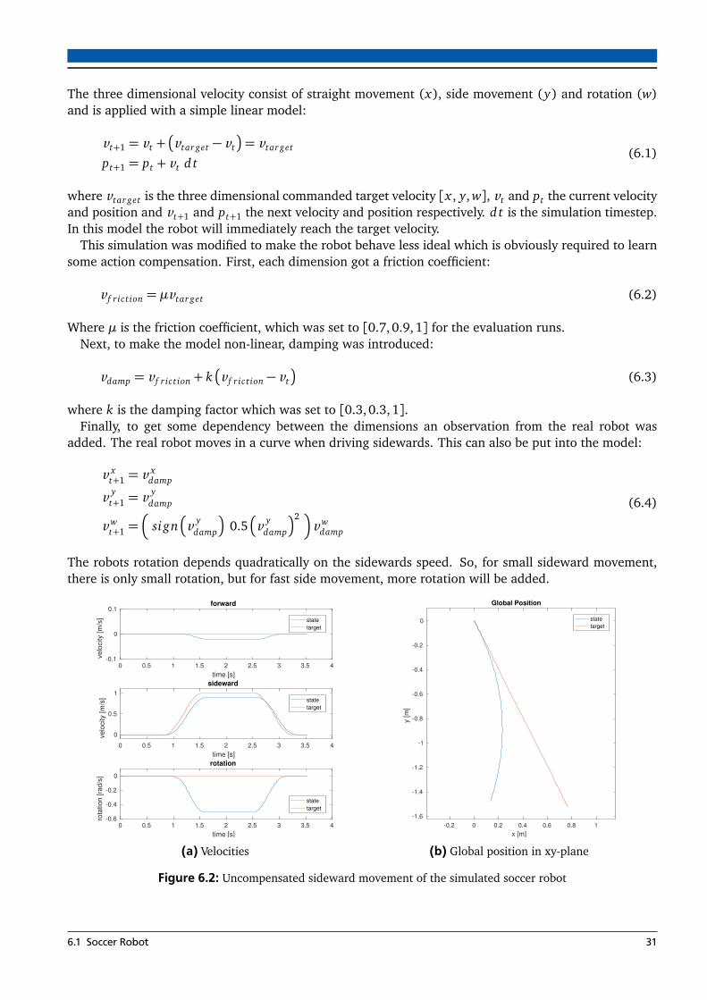
The three dimensional velocity consist of straight movement (x), side movement (y) and rotation (w)and is applied with a simple linear model:

vt+1 = vt +�

vtar get − vt

�

= vtar get

pt+1 = pt + vt d t(6.1)

where vtar get is the three dimensional commanded target velocity [x , y, w], vt and pt the current velocityand position and vt+1 and pt+1 the next velocity and position respectively. d t is the simulation timestep.In this model the robot will immediately reach the target velocity.

This simulation was modified to make the robot behave less ideal which is obviously required to learnsome action compensation. First, each dimension got a friction coefficient:

v f r ic t ion = µvtar get (6.2)

Where µ is the friction coefficient, which was set to [0.7, 0.9,1] for the evaluation runs.Next, to make the model non-linear, damping was introduced:

vdamp = v f r ic t ion + k�

v f r ic t ion − vt

�

(6.3)

where k is the damping factor which was set to [0.3, 0.3,1].Finally, to get some dependency between the dimensions an observation from the real robot was

added. The real robot moves in a curve when driving sidewards. This can also be put into the model:

v xt+1 = v x

damp

v yt+1 = v y

damp

v wt+1 =

�

si gn�

v ydamp

�

0.5�

v ydamp

�2 �

v wdamp

(6.4)

The robots rotation depends quadratically on the sidewards speed. So, for small sideward movement,there is only small rotation, but for fast side movement, more rotation will be added.

0 0.5 1 1.5 2 2.5 3 3.5 4

time [s]

-0.1

0

0.1

ve

locity [

m/s

]

forward

state

target

0 0.5 1 1.5 2 2.5 3 3.5 4

time [s]

0

0.5

1

ve

locity [

m/s

]

sideward

state

target

0 0.5 1 1.5 2 2.5 3 3.5 4

time [s]

-0.6

-0.4

-0.2

0

rota

tio

n [

rad

/s]

rotation

state

target

(a) Velocities

-0.2 0 0.2 0.4 0.6 0.8 1

x [m]

-1.6

-1.4

-1.2

-1

-0.8

-0.6

-0.4

-0.2

0

y [m

]

Global Position

state

target

(b) Global position in xy-plane

Figure 6.2: Uncompensated sideward movement of the simulated soccer robot

6.1 Soccer Robot 31

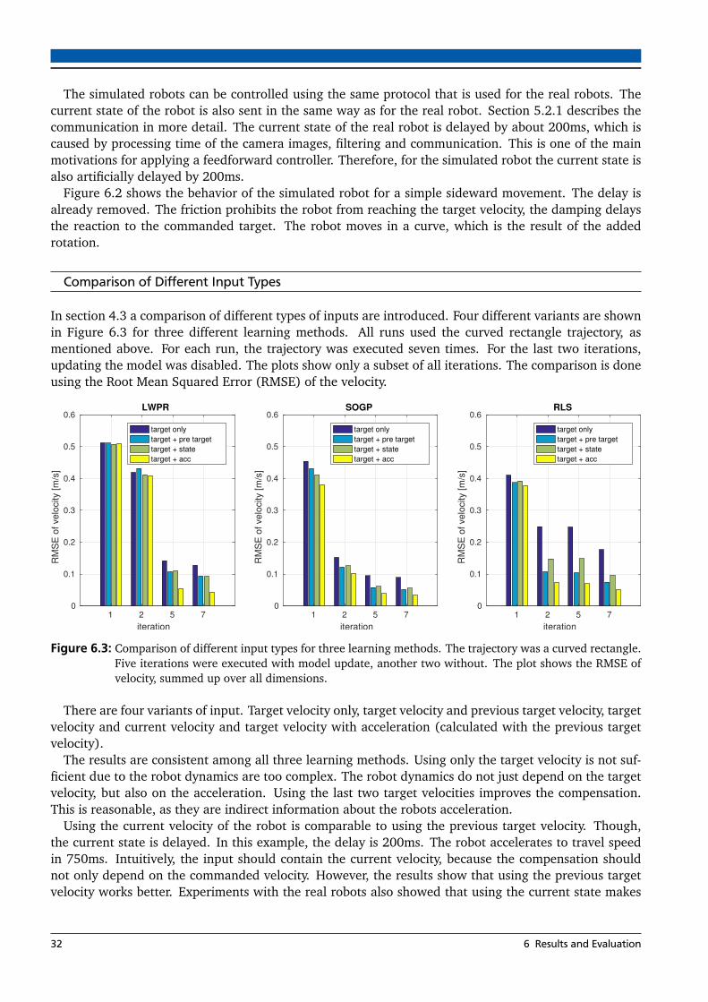
The simulated robots can be controlled using the same protocol that is used for the real robots. Thecurrent state of the robot is also sent in the same way as for the real robot. Section 5.2.1 describes thecommunication in more detail. The current state of the real robot is delayed by about 200ms, which iscaused by processing time of the camera images, filtering and communication. This is one of the mainmotivations for applying a feedforward controller. Therefore, for the simulated robot the current state isalso artificially delayed by 200ms.

Figure 6.2 shows the behavior of the simulated robot for a simple sideward movement. The delay isalready removed. The friction prohibits the robot from reaching the target velocity, the damping delaysthe reaction to the commanded target. The robot moves in a curve, which is the result of the addedrotation.

Comparison of Different Input Types

In section 4.3 a comparison of different types of inputs are introduced. Four different variants are shownin Figure 6.3 for three different learning methods. All runs used the curved rectangle trajectory, asmentioned above. For each run, the trajectory was executed seven times. For the last two iterations,updating the model was disabled. The plots show only a subset of all iterations. The comparison is doneusing the Root Mean Squared Error (RMSE) of the velocity.

1 2 5 7

iteration

0

0.1

0.2

0.3

0.4

0.5

0.6

RM

SE

of

ve

locity [

m/s

]

LWPR

target only

target + pre target

target + state

target + acc

1 2 5 7

iteration

0

0.1

0.2

0.3

0.4

0.5

0.6

RM

SE

of

ve

locity [

m/s

]

SOGP

target only

target + pre target

target + state

target + acc

1 2 5 7

iteration

0

0.1

0.2

0.3

0.4

0.5

0.6

RM

SE

of

ve

locity [

m/s

]

RLS

target only

target + pre target

target + state

target + acc

Figure 6.3: Comparison of different input types for three learning methods. The trajectory was a curved rectangle.Five iterations were executed with model update, another two without. The plot shows the RMSE ofvelocity, summed up over all dimensions.

There are four variants of input. Target velocity only, target velocity and previous target velocity, targetvelocity and current velocity and target velocity with acceleration (calculated with the previous targetvelocity).

The results are consistent among all three learning methods. Using only the target velocity is not suf-ficient due to the robot dynamics are too complex. The robot dynamics do not just depend on the targetvelocity, but also on the acceleration. Using the last two target velocities improves the compensation.This is reasonable, as they are indirect information about the robots acceleration.

Using the current velocity of the robot is comparable to using the previous target velocity. Though,the current state is delayed. In this example, the delay is 200ms. The robot accelerates to travel speedin 750ms. Intuitively, the input should contain the current velocity, because the compensation shouldnot only depend on the commanded velocity. However, the results show that using the previous targetvelocity works better. Experiments with the real robots also showed that using the current state makes

32 6 Results and Evaluation

the prediction less smooth. The current velocity will always contain some noise. The noise will bepropagated through the model to the action command, resulting in noisy commands.

Finally, the input was complemented by the current acceleration. It can be easily calculated using thecurrent and previous target velocity and the time difference. The timestamp is provided by the actioncommand, so the calculated acceleration will match exactly the commanded one and should be smoothas long as the original action was smooth as well. Thus, there is no noise that could be propagated tothe compensation. Providing the acceleration reduces the RMSE significantly compared to only usingthe target velocity and outperforms the other methods as well.

Figure 6.4 shows an excerpt of the trajectory from the last iteration of the LWPR run, shown before.On the left, the input only includes the target velocity, on the right, it also includes the acceleration. Thecompensation, that is returned by the learning method, is also included in the plot.

The plots show the observations, that were mentioned before. Without acceleration, the velocity can becompensated such that it reaches the desired value in a plateau. But during acceleration, the simulateddamping can not be compensated. With acceleration in the input, the damping component can also becompensated.

1.5 2 2.5 3 3.5 4 4.5

time [s]

-1

0

1

ve

locity [

m/s

]

forward - target only

state

target

comp.

1.5 2 2.5 3 3.5 4 4.5

time [s]

0

0.5

1

ve

locity [

m/s

]

sideward - target only

state

target

comp.

1.5 2 2.5 3 3.5 4 4.5

time [s]

0

0.2

0.4

0.6

rota

tio

n [

rad

/s]

rotation - target only

state

target

comp.

1 1.5 2 2.5 3 3.5 4

time [s]

-1

0

1

ve

locity [

m/s

]

forward - target + acc

state

target

comp.

1 1.5 2 2.5 3 3.5 4

time [s]

0

0.5

1

ve

locity [

m/s

]

sideward - target + acc

state

target

comp.

1 1.5 2 2.5 3 3.5 4

time [s]

0

0.2

0.4

0.6

rota

tio

n [

rad

/s]

rotation - target + acc

state

target

comp.

Figure 6.4: Comparison between input with and without acceleration. The left plots show an excerpt of thetrajectory from the last iteration of a LWPR run with the curved rectangle trajectory with only thetarget velocity in the input. The right plots show the same setup, except with acceleration in the input.The individual plots show the target velocity, the actual state and the compensation that is returnedfrom the compensation model.

Comparison of Learning Methods

The trajectories introduced above were applied to three different learning methods, LWPR, SOGP andRLS. Figure 6.5 shows the compensated movement after five iterations for each method. For reference,the uncompensated behavior is also shown.

The best tracking is achieved by SOGP, followed by LWPR which had difficulties to track the startrajectory. RLS, the method with the simplest model, compensates errors significantly, but still has majordivergences compared to the other two methods. This is due to the simple linear model, which can not

6.1 Soccer Robot 33

Figure 6.5: The plots show the movement result for different methods for the three introduced trajectories. Resultsfrom the fifth iteration for each method was chosen.

cover any non-linearity’s. Especially the additional rotation that is based on the sideward speed in thesimulation cannot be handled and will thus result in insufficient rotational compensation.

LWPR uses linear models internally, but can combine them to approximate any non-linear function,while SOGP is based on a Gaussian kernel. The results show, that the kernel is slightly better.

Figure 6.6 shows the full results of the evaluations described before. The Root Mean Squared Erroris used to compare the methods over multiple iterations. A simple proportional feedback controller wasadditionally added for reference. The evaluation setup is the same as in the previous figures, with fiveiterations each with one using model update and two without. The RMSE is calculated per dimensionand summed up.

The results for different trajectories are similar. A major difference between them is the duration, thecurved rectangle takes 8 seconds, the circle 14 seconds and the star 63 seconds.

As already shown in the previous figure, SOGP is the best method followed by LWPR and RLS. Thisis already true for the second iteration. RLS is slightly better in the beginning, as can be seen in theshortest trajectory. LWPR is even worse than the feedback controller in the beginning. It does not workwell for few seen data samples and generates some unproductive compensation in the beginning, butworks with more data.

It can also be seen, that the feedback controller has still a significantly higher error compared to allthree methods.

The last two iterations in the figure were done without updating the model to force the controllers toonly work with their current model. LWPR and SOGP have approximately the same error in iteration sixand seven as in iteration five. RLS has a simple model that is updated continually. This results in a worseresult in the last two iterations than in iteration five.

Processing Time

The processing time is an important criterion for practical application of the method. It can be splitinto two components, the time for updating the model and the time for predicting a compensation. Theupdate time is not as important as the prediction time, because updates are done asynchronically, butthe prediction delays the execution of commands and should thus be low.

34 6 Results and Evaluation

1 2 3 4 5 6 7

iteration

0

0.2

0.4

0.6R

MS

E

Curved Rectangle

none

feedback

LWPR

SOGP

RLS

1 2 3 4 5 6 7

iteration

0

0.2

0.4

0.6

RM

SE

Circle

none

feedback

LWPR

SOGP

RLS

1 2 3 4 5 6 7

iteration

0

0.2

0.4

0.6

RM

SE

Star

none

feedback

LWPR

SOGP

RLS

Figure 6.6: The figures show the RMSE for different learning methods and for different trajectories from simu-lation. Additionally, the RMSE for uncompensated execution and for a simple feedback controller isshown for reference. In all runs, the last two iterations were executed without model update.

Figure 6.7 shows processing time for different learning methods and different trajectories. The testswere run in simulation on a computer with a mobile Intel i7 CPU with 2.6 GHz. The timings for the realsoccer robot are comparable, though there were some results missing for RLS due to unstable behaviors,so the simulated results were used instead.

It can be seen, that the processing time depends on the type of trajectory. The more complex thetrajectory, the more has to be covered by the compensation model and thus, complexity and processingtime increases. The processing time does not depend on the runtime. After the first iteration, it is alreadyat a constant level.

The update time of SOGP is significantly larger than for the other methods. Gaussian Process is knownto be rather small, because of the internal matrix inversion. SOGP keeps the processing time low byremoving data samples that do not add sufficient information, but it is still not fast. The prediction timeis much faster. It only requires a matrix multiplication, no inversion. Still, it slower than LWPR and RLS.

LWPR is the fastest of all three methods with an average prediction time of 65µs and update time of100µs for the star trajectory.

All methods can be considered sufficiently fast. If the control cycle has a frequency of 1kHz, onecontrol step may not take more than 1ms. The highest prediction time of all methods was about 0.5ms.The update is done asynchronically and with an update rate that is based on state updates. A fast sensor,like a gyroscope, can have an update rate of about 1kHz which would be too fast for SOGP, but stilltractable for LWPR and RLS. The evaluated robots had states based on vision and laser scanners whichhave an update rate of about 30 to 100 fps, giving 10 to 33ms processing time. This would be enougheven for SOGP.

6.1 Soccer Robot 35

Figure 6.7: Processing Time for different learning methods in simulation. Processing time is split into update andprediction time. The last two iterations were done without updating the model.

6.1.3 Real Soccer Robot

The real soccer robot was controlled in the same way as the simulated one. The robot receives velocitycommands and uses an internal kinematics model to calculate wheel velocities. Feedback controllerswere turned off. The velocity was directly applied to the wheels without any filtering except for an uppervelocity limit for safety reasons. The wheels itself where controlled with odometry feedback.

The evaluation was done with the trajectories introduced above. Additionally, the robot was driven toan initial pose on the field after each iteration using move_base. This was necessary, because the testfield had limited space and the trajectories ignore any field boundaries. The affw controller was not usedfor driving back to the initial pose, to ensure comparability of individual iterations.

Issues with the Real Robot

During the development process, there were some issues with the real robot, that influenced the perfor-mance of the adaptive controller.

First, it turned out that there was an error in the transformation from the global velocity as receivedfrom the cameras to robot local velocity. When the robot performed a curve movement with a constantforward and rotation velocity, a sideward movement was detected. The adaptive controller tried to com-pensate this sideward movement, but as there was no real side movement, the robot moved sidewardsafterwards. The controller can obviously not work correctly, if the given state is wrong. For this reason,it is very important to verify that the reference state is reasonable.

Also, the detection of the orientation of the robot from the cameras was not very accurate and differ-entiation to velocity produced a very noise signal. In order to detect more fine grained rotations, the

36 6 Results and Evaluation

gyroscope on the robot was used for rotation velocity. This improved the quality of the rotation inputsignificantly.

Another important parameter is the delay of the state. The soccer robot has a very high delay of about200ms. Due to the distributed system that is not part of ROS, there are no timestamps available thatcould be used to detect the delay automatically. Setting the delay wrong can have major influence tothe performance of the controller. Without setting a delay, the adaptive controller would compare targetand measured state at a wrong time, resulting in unpredictable and unwanted behavior. Section 5.2.3describes this issue in detail.

Real Robot Behavior with and without Compensation

The behavior of the real robot is obviously a little bit different compared to the simulation. Figure 6.8shows the circle trajectory without compensation. During one iteration, the robot rotates 90° due to theslippage of the wheels that occur during the circular movement. The velocity plot shows that the robotrotates especially during sidewards movement.

Figure 6.9 illustrates the same trajectory after five iterations of LWPR. It should be noted, that as thereis no feedback controller on position level, thus all control errors are accumulating over time. Althoughthe position error is not used as reference, if the measured velocity is incorrect as well, the robot will notlearn the correct compensation for exactly tracking the desired trajectory.

It can be seen from velocity and position plot that during this experiment the orientation is close tothe target with exception for some noise. The forward and sideward velocity fits the target velocity welland on position layer, there is a final error of about 20cm.

Comparison of Learning Methods

In section 6.1.2 the methods were already compared for the simulation. Experiments with the real robotshowed similar results, but also some major differences. The results are shown in Figure 6.10.

First, the feedback controller did not work well. It showed no improvement over uncompensatedcontrol and resulted in even worse results for the circle trajectory. It turned out that this is mainly dueto differences in the rotation. While it can improve tracking on the x and y dimensions, it producesoscillations on the rotation dimension. The rotation is prone to high noise and has sudden non-linear

0 2 4 6 8 10 12 14

time [s]

-1

0

1

ve

locity [

m/s

]

forward

state

target

0 2 4 6 8 10 12 14

time [s]

-1

0

1

ve

locity [

m/s

]

sideward

state

target

0 2 4 6 8 10 12 14

time [s]

-0.2

0

0.2

0.4

0.6

rota

tio

n [

rad

/s]

rotation

state

target

(a) Velocities

-0.2 0 0.2 0.4 0.6 0.8 1 1.2 1.4

x [m]

0

0.2

0.4

0.6

0.8

1

1.2

1.4

1.6

1.8

y [m

]

Global Position

state

target

(b) Global position in xy-plane

Figure 6.8: Uncompensated circle trajectory with the real soccer robot.

6.1 Soccer Robot 37

0 2 4 6 8 10 12 14

time [s]

-2

-1

0

1

ve

locity [

m/s

]forward

state

target

comp.

0 2 4 6 8 10 12 14

time [s]

-2

-1

0

1

ve

locity [

m/s

]

sideward

state

target

comp.

0 2 4 6 8 10 12 14

time [s]

-1

-0.5

0

rota

tio

n [

rad

/s]

rotation

state

target

comp.

(a) Velocities

0 0.2 0.4 0.6 0.8 1 1.2 1.4 1.6

x [m]

-0.4

-0.2

0

0.2

0.4

0.6

0.8

1

1.2

1.4

y [m

]

Global Position

state

target

(b) Global position in xy-plane

Figure 6.9: Circle trajectory with the real soccer robot after five iterations with LWPR. The velocity plots also showthe compensation term that is calculated by LWPR to compensate the movement.

changes, while x and y dimensions are smoother. The delay of 200ms causes a high reaction time.Rotation compensations are thus usually too late and can cause undesired behavior.

The feedback controller is designed to be similar to the learning methods. It uses the same delay andthe same compensation terms that would be used for the learning methods. A well designed feedbackcontroller would rather work on a predicted current state than on the true delayed state. However, thefeedback controller helps understanding the results of RLS.

While LWPR and SOGP show comparable results to the simulation, RLS does not work well. For thecurved rectangle, the best results are achieved in the last two iterations, when model updates weredisabled. The previous iterations and all iterations from the circle trajectory are worse than withoutcompensation.

Previous experiments in simulation showed, that the RLS model is too simple to model the rotationcompensation and needs to adapt continually. A forgetting factor is used for setting the adaption speed.A higher value may improve the results, but setting the factor too high will slow down convergence toothe optimal compensation term. Additionally, the model needs to continually adapt due to its simplicity,so a low forgetting rate would be inappropriate.

In the experiment, a forgetting factor λ = 0.99 was used. Detailed analysis of the RLS runs showed,that it reacted similar to the feedback controller. It was not able to build a model that captures thecompensation terms correctly, resulting in continual adaption that degenerates the behavior similar tothe feedback controller.

RLS was thus not applied to the star shape, as this has resulted in unstable behavior and therefore nopromising results were expected given the results of the simpler trajectories.

LWPR and SOGP performed indeed well. Figure 6.11 shows the results of all methods after fiveiterations.

LWPR did not work well with few data samples. The prediction of compensation terms can get veryspiky causing the robot to move uncontrollable. SOGP is better at dealing with few data, but in general,it is better for all methods to start prediction after they have seen a reasonable amount of data, so theycan not generate harmful compensation predictions. For this reason, the controller has a parametermax_nData = 800 that can be used to skip prediction for the first 800 samples. As the controller shouldbe used online over a longer period of time, this is no drawback in terms of the applicability of thecontroller.

38 6 Results and Evaluation

1 2 3 4 5 6 7

iteration

0

0.2

0.4

0.6

0.8

RM

SE

Curved Rectangle

none

feedback

LWPR

SOGP

RLS

1 2 3 4 5 6 7

iteration

0

0.5

1

1.5

2

RM

SE

Circle

none

feedback

LWPR

SOGP

RLS

1 2 3 4 5 6 7

iteration

0

0.2

0.4

0.6

0.8

1

RM

SE

Star

none

feedback

LWPR

SOGP

Figure 6.10: The plots show the RMSE for different learning methods and for different trajectories for the real soc-cer robot. Additionally, the RMSE for uncompensated execution and for a simple feedback controlleris shown for reference. In all runs, the last two iterations were executed without model update.

Evaluation of Performance on a Major Malfunction

The biggest motivation to use an adaptive controller is that it can react automatically to malfunctions.In order to test this, the motor of the rear right wheel was electrically disconnected, so that the wheelcould still move freely. This simulated malfunction causes the robot to drive in a curve, when forwardmovement is commanded.

The first task was to drive in a straight line back and forth, starting with an empty model. Figure 6.12shows the continuous improvement, using LWPR and SOGP. The first plot shows the uncompensated trialwhere the robot performs an expected curved movement. The wheels are not attached symmetrically,so the backwards movement differs from the forward movement. This is why the robot will not arriveon its initial position, though the trajectory of the backwards movement is simply the negative forwardtrajectory.

The experiments show, that SOGP is not able to fully compensate the movement. LWPR with defaultparameters showed similar results to SOGP, but it has a build in forgetting factor that can be tuned.It turned out, that the forgetting factor was too large. The compensation model requires adaptation,because the action compensation is iteratively approximated. If the compensation term is not achievedwithin some samples, the learning methods need to forget the previous ones. LWPR achieves this bysetting an initial forgetting factor λ to each receptive field. This factor is further increased over time, if

6.1 Soccer Robot 39

Figure 6.11: The plots show the movement result for different methods for the three introduced trajectories. Re-sults from the fifth iteration for each method was chosen.

0 1 2

x [m]

-0.5

0

0.5

1

y [

m]

no compensation

LWPR

0 1 2

x [m]

-1

-0.5

0

0.5

y [

m]

1st iteration

0 1 2

x [m]

-0.5

0

0.5

1

y [

m]

2nd iteration

0 1 2

x [m]

-0.5

0

0.5

1

y [

m]

3rd iteration

0 1 2

x [m]

-0.5

0

0.5

1

y [

m]

4th iteration

state

target

0 1 2

x [m]

-0.5

0

0.5

1

y [

m]

SOGP

0 1 2

x [m]

-1

-0.5

0

0.5

y [

m]

0 1 2

x [m]

-0.5

0

0.5

1

y [

m]

0 1 2

x [m]

-0.5

0

0.5

1

y [

m]

0 1 2

x [m]

-0.5

0

0.5

1

y [

m]

Figure 6.12: Robot behavior, when rear right wheel is disconnected.

more data is associated with the receptive field. For the experiment, the factor was changed to λini t =0.99, λ f inal = 0.999.

SOGP has no notion of forgetting. The model is based on data samples that causes compensationterms that have not converged to the correct value will stay within the model until sufficient new datawas inserted into the model to remove the old data sample. The model will slowly adapt, but theadaptation speed can not easily be influenced.

The assumption, that the missing notion of forgetting caused insufficient compensation, was provedby continuing the experiment. The learned models for LWPR and SOGP were reused, but the motor wasreconnected again, so that the robot would move straight again without compensation.

Figure 6.13 shows the result of this experiment. The compensation within the models cause the robotto turn towards the opposite direction now, because there is still a compensation within the model. LWPRadapted after the first iteration, but SOGP could not recover even after the fifth iteration. It can be seenthough, that it converges slowly towards straight movement. This supports the previously explainedassumption, that the model can only slowly forget data, because it is only based on data samples.

40 6 Results and Evaluation

0 1 2

x [m]

-1

-0.5

0

0.5

y [

m]

1st iteration

LWPR

0 1 2

x [m]

-1

-0.5

0

0.5

y [

m]

2nd iteration

0 1 2

x [m]

-1

0

1

y [

m]

3rd iteration

0 1 2

x [m]

-1

0

1

y [

m]

4th iteration

0 1 2

x [m]

-1

0

1

y [

m]

5th iteration

state

target

0 1 2

x [m]

-1.5

-1

-0.5

0

y [

m]

SOGP

0 1 2

x [m]

-1.5

-1

-0.5

0y [

m]

0 1 2

x [m]

-1.5

-1

-0.5

0

y [

m]

0 1 2

x [m]

-1.5

-1

-0.5

0

y [

m]

0 1 2

x [m]

-1.5

-1

-0.5

0

0.5

y [

m]

Figure 6.13: Robot behavior, when rear right wheel is reconnected after model has learned compensation of dis-connected wheel.

6.1.4 Summary

The adaptive controller improves the movement of the soccer robot significantly. The robot showedmotion errors on all three action dimensions. Especially the rotation dimension has major deviationsfrom the target command that depends on multiple input dimensions.

While all three learning methods showed improvements in simulation, it turned out that on the realrobot, RLS was too simplistic to improve movement. Further analysis of LWPR and SOGP with a simu-lated malfunction showed, that SOGP suffers from its sample based model. A forgetting mechanism ismissing that would control how fast the model can be adapted to new situations. LWPR can be tuned toreact very fast to a system change.

In terms of processing time, all methods were fast enough to be applicable in a high speed controller.Though, SOGP is significantly slower compared to LWPR.

6.2 Rescue Robot

The second robot platform that was evaluated differs significantly from the omnidirectional soccer robot.It has a tracked differential drive. This means, it can drive forward and backward on the first actiondimension and rotate on the second one. Those dimensions are also the only dimensions where errorscan be compensated. The robot is larger and much heavier and interacts in a completely differentenvironment.

The tracked vehicles is actuated by two tracks with odometry sensors for controlling rotation speed.Driving forward on an even floor does not produce noticeable slippage and the motion model will thusbe accurate, but rotation in place or driving curves induces significant slippage between ground andtracks. The robot will also operate in uneven terrain. It has an IMU that measures the pose of the robot,which can be used as additional input to the adaptive controller.

This section is structured similar to the previous one. First, trajectories for evaluation are introduced.Afterwards, results for the real robot are shown. There was also a simulation for the robot, but it wasnot used for evaluation, because the methods were already evaluated in detail for the soccer robot andspecial behavior like sloping position was not available in the simulation.

6.2.1 Trajectories

There are three trajectories that were used for the evaluation that are shown in Figure 6.14. The firsttrajectory is a simple 360° rotation in place. The rotation speed was constant with a smooth acceler-

6.2 Rescue Robot 41

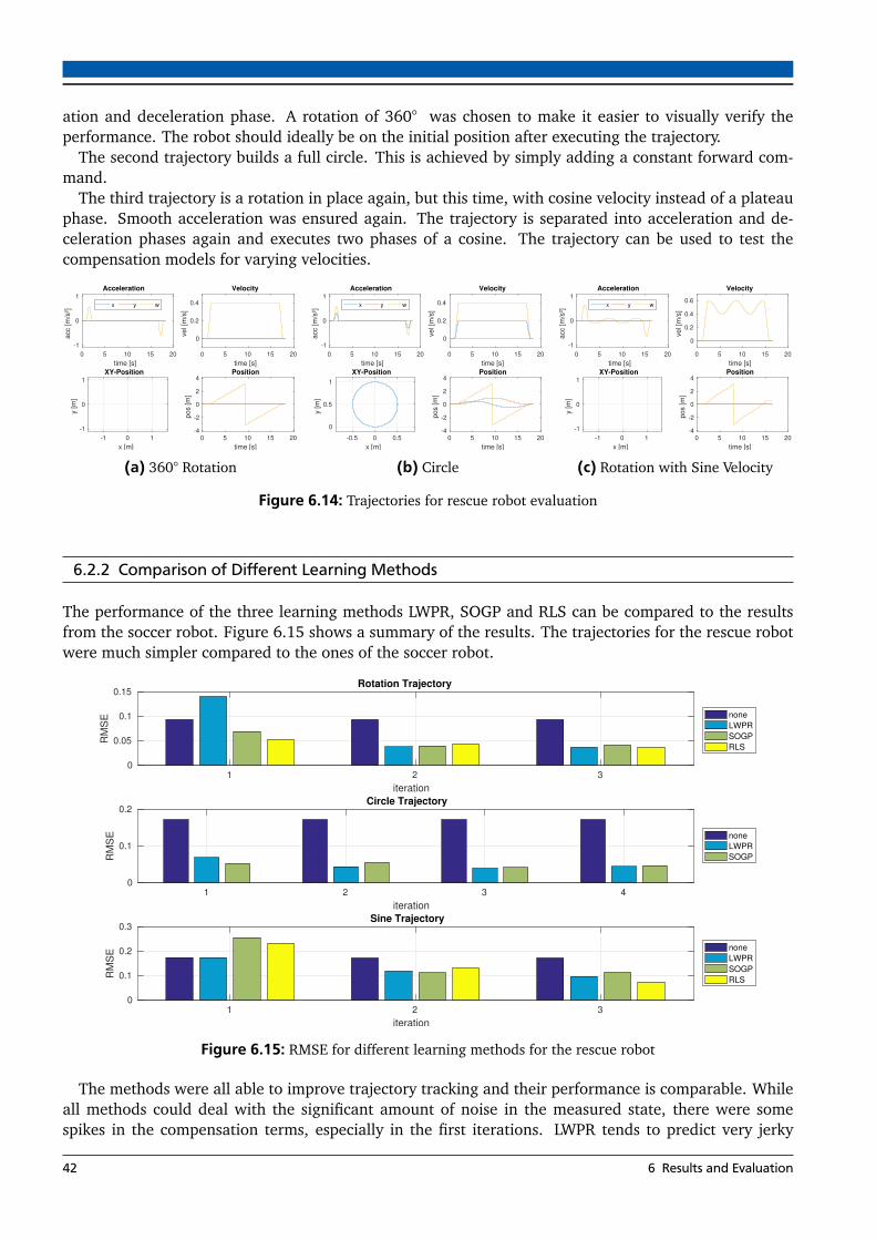
ation and deceleration phase. A rotation of 360° was chosen to make it easier to visually verify theperformance. The robot should ideally be on the initial position after executing the trajectory.

The second trajectory builds a full circle. This is achieved by simply adding a constant forward com-mand.

The third trajectory is a rotation in place again, but this time, with cosine velocity instead of a plateauphase. Smooth acceleration was ensured again. The trajectory is separated into acceleration and de-celeration phases again and executes two phases of a cosine. The trajectory can be used to test thecompensation models for varying velocities.

0 5 10 15 20

time [s]

-1

0

1

acc [

m/s

²]

Acceleration

x y w

0 5 10 15 20

time [s]

0

0.2

0.4

ve

l [m

/s]

Velocity

-1 0 1

x [m]

-1

0

1

y [

m]

XY-Position

0 5 10 15 20

time [s]

-4

-2

0

2

4

po

s [

m]

Position

(a) 360° Rotation

0 5 10 15 20

time [s]

-1

0

1

acc [

m/s

²]

Acceleration

x y w

0 5 10 15 20

time [s]

0

0.2

0.4

ve

l [m

/s]

Velocity

-0.5 0 0.5

x [m]

0

0.5

1

y [

m]

XY-Position

0 5 10 15 20

time [s]

-4

-2

0

2

4

po

s [

m]

Position

(b) Circle

0 5 10 15 20

time [s]

-1

0

1

acc [

m/s

²]

Acceleration

x y w

0 5 10 15 20

time [s]

0

0.2

0.4

0.6

ve

l [m

/s]

Velocity

-1 0 1

x [m]

-1

0

1

y [

m]

XY-Position

0 5 10 15 20

time [s]

-4

-2

0

2

4

po

s [

m]

Position

(c) Rotation with Sine Velocity

Figure 6.14: Trajectories for rescue robot evaluation

6.2.2 Comparison of Different Learning Methods

The performance of the three learning methods LWPR, SOGP and RLS can be compared to the resultsfrom the soccer robot. Figure 6.15 shows a summary of the results. The trajectories for the rescue robotwere much simpler compared to the ones of the soccer robot.

1 2 3

iteration

0

0.05

0.1

0.15

RM

SE

Rotation Trajectory

none

LWPR

SOGP

RLS

1 2 3 4

iteration

0

0.1

0.2

RM

SE

Circle Trajectory

none

LWPR

SOGP

1 2 3

iteration

0

0.1

0.2

0.3

RM

SE

Sine Trajectory

none

LWPR

SOGP

RLS

Figure 6.15: RMSE for different learning methods for the rescue robot

The methods were all able to improve trajectory tracking and their performance is comparable. Whileall methods could deal with the significant amount of noise in the measured state, there were somespikes in the compensation terms, especially in the first iterations. LWPR tends to predict very jerky

42 6 Results and Evaluation

output, if it does not have enough data, so prediction was delayed until about 800 data samples hadarrived.

SOGP turned out to rely on good hyperparameters. The bandwidth of the kernel has an impact on thestability of the kernel and can cause singularities which result in NaN values in the prediction output,destroying the whole model.

The performance of RLS mainly depends on the forgetting factor. Setting it too low (high forgettingrate) lets the model react too much on noisy data, while setting it too low will delay the reaction onchanges.

Using more complex trajectories would have been more complicated than for the soccer robot, be-cause the large robot requires more space and can be damaged or damage its environment more easily.Complex trajectories were thus only tested with the soccer robot. Instead, there is an experiment thatuses additional custom states for the learning methods, described below. Results of this experiment areskipped here.

6.2.3 Simple Rotation

The experiments with the rotation trajectory on flat ground showed that the compensation can beadapted after the first iteration, even in the presence of noise. SOGP and RLS predicted first reason-able adaptations before the end of the first iteration. The prediction of LWPR with few data samples isunreliable, thus the first iteration was worse than without compensation. In later experiments, predictionwas blocked until a sufficient amount of data was recorded.

Spikes in the forward dimension can cause sudden jumps forward or backward. The longer the adap-tive controller runs, the less likely this happens, because sufficient data supports the certainty, that thespike is a measurement error.

The measured global position of the rotation is not constant, but builds a small circle of about 10cmdiameter. Further experiments showed that this depends on the flipper positions, which influence thearea of the tracks that touch the ground. Lowering the flippers, so that they are horizontal, lets the robotturn in a large circle of about half a meter diameter. Raising the flippers resulted in bad sensor data,because the flippers handicapped the laser sensor.

The circle movement during a rotation can not be compensated, because it is a result of sidewardsslippage.

6.2.4 Moving in a Circle

The circle trajectory, introduced before, should show the ability of the controller to compensate on bothaction dimensions. It was executed on an even floor. Figure 6.16 shows the position tracking of thetrajectory for uncompensated movement and for compensated movement with SOGP and LWPR afterfour iterations.

-0.5 0 0.50

0.2

0.4

0.6

0.8

1no comp.

-0.5 0 0.50

0.2

0.4

0.6

0.8

1

LWPR

-0.5 0 0.5

0

0.2

0.4

0.6

0.8

1

SOGP

target

measured

start

Figure 6.16: Position tracking of the circle trajectory with LWPR and SOGP.

6.2 Rescue Robot 43

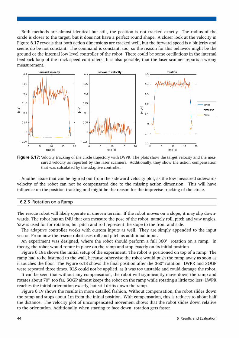
Both methods are almost identical but still, the position is not tracked exactly. The radius of thecircle is closer to the target, but it does not have a perfect round shape. A closer look at the velocity inFigure 6.17 reveals that both action dimensions are tracked well, but the forward speed is a bit jerky andseems do be not constant. The command is constant, too, so the reason for this behavior might be theground or the internal low level controller of the robot. There could be some oscillations in the internalfeedback loop of the track speed controllers. It is also possible, that the laser scanner reports a wrongmeasurement.

Figure 6.17: Velocity tracking of the circle trajectory with LWPR. The plots show the target velocity and the mea-sured velocity as reported by the laser scanners. Additionally, they show the action compensationthat was calculated by the adaptive controller.

Another issue that can be figured out from the sideward velocity plot, as the low measured sidewardsvelocity of the robot can not be compensated due to the missing action dimension. This will haveinfluence on the position tracking and might be the reason for the imprecise tracking of the circle.

6.2.5 Rotation on a Ramp

The rescue robot will likely operate in uneven terrain. If the robot moves on a slope, it may slip down-wards. The robot has an IMU that can measure the pose of the robot, namely roll, pitch and yaw angles.Yaw is used for for rotation, but pitch and roll represent the slope to the front and side.

The adaptive controller works with custom inputs as well. They are simply appended to the inputvector. From now the rescue robot uses roll and pitch as additional input.

An experiment was designed, where the robot should perform a full 360° rotation on a ramp. Intheory, the robot would rotate in place on the ramp and stop exactly on its initial position.

Figure 6.18a shows the initial setup of the experiment. The robot is positioned on top of a ramp. Theramp had to be fastened to the wall, because otherwise the robot would push the ramp away as soon asit touches the floor. The Figure 6.18 shows the final position after the 360° rotation. LWPR and SOGPwere repeated three times. RLS could not be applied, as it was too unstable and could damage the robot.

It can be seen that without any compensation, the robot will significantly move down the ramp androtates about 70° too far. SOGP almost keeps the robot on the ramp while rotating a little too less. LWPRreaches the initial orientation exactly, but still drifts down the ramp.

Figure 6.19 shows the results in more detailed fashion. Without compensation, the robot slides downthe ramp and stops about 1m from the initial position. With compensation, this is reduces to about halfthe distance. The velocity plot of uncompensated movement shows that the robot slides down relativeto the orientation. Additionally, when starting to face down, rotation gets faster.

44 6 Results and Evaluation

(a) Init (b) no comp. (c) LWPR (d) SOGP

Figure 6.18: Initial and final position on a 360° Rotation on a ramp with LWPR and SOGP.

-0.4 -0.2 0

y [m]

-1

-0.9

-0.8

-0.7

-0.6

-0.5

-0.4

-0.3

-0.2

-0.1

0

0.1

x [m

]

Global Position

none

LWPR

SOGP

target

action comp.

(a) Global position

0 5 10 15 20

time [s]

-0.2

0

0.2

[m/s

]

forward

0 5 10 15 20

time [s]

-0.2

0

0.2

[m/s

]

sideward

0 5 10 15 20

time [s]

-0.5

0

0.5

1

[rad/s

]

rotation

(b) Uncompensated velocity

0 5 10 15 20

time [s]

-0.2

0

0.2

[m/s

]

forward

0 5 10 15 20

time [s]

-0.2

0

0.2

[m/s

]

sideward

0 5 10 15 20

time [s]

-0.5

0

0.5

1

[rad/s

]

rotation

(c) LWPR velocity

0 5 10 15 20

time [s]

-0.2

0

0.2

[m/s

]

forward

0 5 10 15 20

time [s]

-0.2

0

0.2

[m/s

]

sideward

0 5 10 15 20

time [s]

-0.5

0

0.5

1

[rad/s

]

rotation

(d) SOGP velocity

Figure 6.19: 360° rotation on a ramp with LWPR, SOGP and without compensation.

6.2 Rescue Robot 45

The velocity plots of the learning methods demonstrate that forward and rotational velocity is com-pensated correctly, so that both actions fit to the commanded target. The magenta colored line showsthe used action compensation from the individual models.

The reason for the large distance that the robot still slides down is the occurring sidewards movement.The robot can obviously also slide sidewards, but there is no possibility to compensate this with theadaptive controller.

6.2.6 Summary

All three methods performed well during the evaluations. They showed similar issues as with the soccerrobot. LWPR requires sufficient data to predict smooth compensations and performance of SOGP andRLS depend on the selection of certain parameters.

Even though the measured velocities were very jerky and noisy, this did not influence the performanceof the adaptive controller, given that the controller has seen sufficient data in past.

In contrast to the soccer robot, the rescue robot only used two instead of three action dimensions, butadditionally got two custom inputs, the roll and pitch angles from IMU. Those additional states wereused to compensate slippage on a ramp. Experiments showed that those inputs supported successfullyto track the reference rotation speed correctly and to reduce slippage down the ramp by about 50%.

Having only two dimensions for compensation turned out to be insufficient to track the desired globalposition. As soon as the robot rotates, there is also a sidewards movement part that is not compensableand adds to the position error. Experiments showed, that the amount of sidewards movement dependson the flipper position and could be reduced by tuning the position of the flipper. The flipper position canbe added as a custom input to the learner so that the compensation can depend on the flipper positionas well, but it can not be used as an additional action command as there is no suitable reference signalthat could be measured. Alternatively, this behavior could be compensated on a higher level of control.

All experiments were done under controlled conditions. As soon as there are external influences thatthe robot can not measure yet, like rough or moving terrain, the controller has no reference on whichit can learn individual behavior and has to adapt continually. In this case, a carefully tuned forgettingfactor is important. LWPR has a good mechanism for this, while SOGP has no notion of forgetting at alland will thus require a lot of data, before adapting. RLS requires fast adaptation due to a very simplelinear model, thus a well tuned forgetting factor is required anyway.

Given a good choice of forgetting capability, the methods should be robust against situations likehitting obstacles, but further tests are required to prove this assumption. It may reasonable to activatethe model update only under controlled conditions, for example during setup, or if bad tracking ofvelocity is detected by the operator.

6.3 Feasibility of the Evaluated Methods

In the previous sections, all three methods (LWPR, SOGP and RLS) were tested on two different robotplatforms in terms of compensation performance and computational complexity. In order to use themethods in practice, their models should also be memory efficient and persistent to avoid relearningeverything after each robot startup. The following subsections describe the memory usage and storageof each method.

6.3.1 LWPR

LWPR is written in C with a strong focus on performance and memory efficiency. It uses batch allocationof memory to avoid frequent calls to malloc. So called receptive fields store the local linear models andare added and pruned in the learning process. If more receptive fields are required than their is memory

46 6 Results and Evaluation

available, a new chunk of memory is allocated. The number of receptive fields depend on the complexityof the model and some hyperparameters such as the distance metric.

The authors of LWPR also implemented their method on a micro controller. The soccer robot has anSTM32F746ZG with 216MHz and 320kB static RAM. During this thesis, the LWPR implementation wasadapted to run on this microcontroller. To save memory, all double variables where converted to float.About 160kB of memory where available. The porting was successful. Model updates and predictionswhere possible, but as soon as the model got more complex, the system ran out of memory. The upperlimit for receptive fields was 16. However, this experiment showed that LWPR can basically run on alow-level system.

LWPR can store the whole model in a binary or XML file. The experiment with the soccer robot and thestar shape required 37 receptive fields for each of the three action dimensions after the seventh iteration,resulting in a binary file size of 241kb.

6.3.2 SOGP

Gaussian Process builds its model on the training data. SOGP is an extension to standard GP, where datais pruned to maintain a maximum amount of data. The maximum capacity was set to 100 during allexperiments. SOGP maintains three matrices: alpha (N x Dout), C (N xN) and Q (N xN) where N is thecapacity and Dout the output dimension. Additionally, it maintains up to N basis vectors (1x Din, whereDin is the input dimension) for checking the novelty of new data. Due to the fixed capacity, the maximummemory usage is limited.

The experiment with the soccer robot and the star shape required 100 basis vectors. The model isstored in a simple text format and required 353kB on disk. In memory, the usage is about 170kB for 6input fields and 3 output fields.

6.3.3 RLS

RLS is based on a linear model and does not need to remember any training data. It uses two matricesto maintain its state: w (1x Din) and P (Din x Din). The memory usage is thus fixed. For 6 input fields,about 450B are required per output dimension. The model is stored in the same text format as SOGPand requires about 2kB per output dimension.

6.3 Feasibility of the Evaluated Methods 47

7 Conclusion

During this thesis, a framework for an adaptive feedforward controller was developed. A ROS-independent library with multiple online learning methods was created and integrated into ROS. Ituses standard messages and is thus easily applicable to new systems. The evaluation was successfullydone on a small omnidirectional soccer robot and a large tracked rescue robot.

The developed adaptive controller is based on a compensation model that is used in conjunction withan existing motion model of the given system. Compared to approaches, which learn the whole motionmodel, the compensation model benefits from being used without any setup phase. As long as there isno data available, the compensation is zero and the default motion model controls the robot.

Multiple methods were analyzed in terms of applicability in the controller and three methods werechosen for further evaluation. All three methods were able to improve the tracking of a given trajectoryand processing time was fast enough to be usable for high speed control.

Recursive Least Squares was the simplest of the three methods. Due to its simple internal model, itcan only store linear dependencies between input and output. While it worked well as long as actioncompensations were almost linear, it showed poor results on more difficult scenarios.

Sparse Online Gaussian Process uses the approximation power of Gaussian Process Regression to fitnon-linear dependencies as well and performed very well especially in simulation. However, it was notable to change the existing model within a reasonable time when the system behavior changed, due tothe purely data-based model. The method can thus not adapt to a major malfunction or a significantchange in terrain.

Locally Weighted Projection Regression turned out to be a very powerful method for online learning.It is fast and achieves good approximation. The build-in forgetting mechanism is important for continualadaption, even if the system behavior changes. One of the major disadvantages of LWPR is its behaviorwhen only few data samples are available, but this is only relevant for newly created models.

The adaptive controller successfully improved the tracking of a reference trajectory for both, the soccerrobot and the rescue robot. The default motion model of the soccer robot produced major rotationdivergences that depended on translational velocity and acceleration when moving. The controller wasable to almost eliminate this divergences after a few repetitions of the same trajectories. Problems wereencountered, when the robot was moved fast and lost contact to ground. However, this can be consideredas a physical limitation of the robot platform.

Evaluations on the rescue robot additionally showed successful usage of additional input dimensions.Using the roll and pitch angles of the robot pose, the robot was able to compensate rotational velocityon a ramp and reduced translational slippage within the robots capabilities. The controller worked welleven in the presence of noisy measurements. One of the major problems on the differential robot wasthe missing third action dimension. Sideward movement due to slippage could be measured, but can notbe compensated directly. This resulted in imprecise position tracking.

49

8 Future Work

The adaptive feedforward controller was applied to two robot platforms. The concept of this controlleris not limited to ground vehicles, but could also be applied to any other system like humanoid robots.Given a model that uses for example a forward velocity command as input and provides sensors formeasuring the resulting velocity, the adaptive controller can be applied as well. In case of a humanoidrobot, the model could calculate the step size based on the commanded velocity.

The input dimension of the controller in the experiments was rather low. More states of the robotplatform could be used. With more information, the compensation model could adapt more specificallyto individual states, such as terrain properties. On large robots, the joint positions may also be relevant.The rescue robot has flippers attached to the tracks that have a major influence on the rotation speedand in uneven terrain, the position of the arm that is attached on top of the robot, may also have aninfluence.

When the controller is initialized with an empty model, prediction of the compensation term can bejerky until sufficient data has been seen. If the prediction is blocked in the beginning, there will be a largejump in the action compensation as soon as the prediction becomes unblocked again. If the robot appliesthe command directly, this can damage the robot in the worst case, but will at least result in short jerkymovement. This does not happen often, but a mechanism to avoid such behavior would be desirable inthe long term. A possible solution could be to add an additional layer that smooths intermediate actioncompensations.

The adaptive controller for the soccer robot had been executed on a remote computer, because therobot only provides a micro-controller at the moment. First attempts to implement LWPR on the micro-controller were successful and showed practical performance even in a control cycle of 1kHz, but thememory size was not sufficient to store the whole model. In the future, a more powerful computer, likea raspberry pi could be added which provides enough computational resources. In the mean time, alook-up table could be used to store a previously learned model.

51

Bibliography

[1] M. C. Choy, D. Srinivasan, and R. L. Cheu, “Neural networks for continuous online learning andcontrol.,” IEEE transactions on neural networks / a publication of the IEEE Neural Networks Council,vol. 17, no. 6, pp. 1511–1531, 2006.

[2] J. Nakanishi, J. A. Farrell, and S. Schaal, “Composite adaptive control with locally weighted statis-tical learning,” Neural Networks, vol. 18, no. 1, pp. 71–90, 2005.

[3] J. Nakanishi and S. Schaal, “Feedback error learning and nonlinear adaptive control,” Neural Net-works, vol. 17, no. 10, pp. 1453–1465, 2004.

[4] R. L. Williams, B. E. Carter, P. Gallina, and G. Rosati, “Dynamic model with slip for wheeled om-nidirectional robots,” IEEE Transactions on Robotics and Automation, vol. 18, no. 3, pp. 285–293,2002.

[5] M. Reinstein, V. Kubelka, and K. Zimmermann, “Terrain adaptive odometry for mobile skid-steerrobots,” Proceedings - IEEE International Conference on Robotics and Automation, pp. 4706–4711,2013.

[6] K. M. Passino, “Intelligent control: an overview of techniques,” Perspectives in Control Engineering:Technologies, Applications, and New Directions, pp. 104–133, 2001.

[7] D. A. Bristow, M. Tharayil, and A. G. Alleyne, “A survey of iterative learning control,” IEEE ControlSystems Magazine, vol. 26, no. June, pp. 96–114, 2006.

[8] K. L. Moore, “Iterative learning control,” 1993.

[9] K. L. Moore, “An Introduction to Iterative Learning Control,” Csm Eges, 2006.

[10] S. Pankaj, “Comparative Analysis of MIT Rule and Lyapunov Rule in Model Reference AdaptiveControl Scheme,” Engineering, vol. 2, no. 4, pp. 154–163, 2011.

[11] D. J. Leith and W. E. Leithead, “Survey of gain-scheduling analysis and design,” International Jour-nal of Control, vol. 73, pp. 1001–1025, 2000.

[12] E. Lavretsky, “Adaptive control: Introduction, overview, and applications,” NASA Adaptive ControlWorkshop. NASA Marshall Space Center, Huntsville, AL, vol. 24, 2009.

[13] D. E. Kirk, Optimal Control Theory: An Introduction. Dover Books on Electrical Engineering, DoverPublications, 2012.

[14] J. L. Martinez, A. Mandow, J. Morales, A. Garcia-Cerezo, and S. Pedraza, “Kinematic modellingof tracked vehicles by experimental identification,” The International Journal of Robotics Research,vol. 24, no. 10, pp. 867–878, 2004.

[15] A. Conceicao, A. Moreira, and P. Costa, “Practical approach of modeling and parameters estima-tion for omnidirectional mobile robots,” Mechatronics, IEEE/ASME Transactions on, vol. 14, no. 3,pp. 377–381, 2009.

[16] A. Gloye, F. Wiesel, O. Tenchio, M. Simon, and R. Rojas, “Robot Heal Thyself - Precise and Fault-Tolerant Control of Imprecise or Malfunctioning Robots,” RoboCup 2005. International Symposium,Osaka, Japan, 2005.

53

[17] A. Gloye, S. Behnke, A. Egorova, F. Wiesel, O. Tenchio, M. Schreiber, and R. Rojas, “Predicting awayrobot control latency,” 2004.

[18] Y. Wu and Z. Yuan, “Motion compensation of omnidirectional wheel robot using neural networks,”pp. 1–5, 2006.

[19] A. Gams, B. Nemec, A. J. Ijspeert, and A. Ude, “Coupling Movement Primitives: Interaction Withthe Environment and Bimanual Tasks,” IEEE Transactions on Robotics, vol. 30, no. 4, pp. 816–830,2014.

[20] A. Gams, M. Denisa, and A. Ude, “Learning of Parametric Coupling Terms for Robot-EnvironmentInteraction,” pp. 304–309, 2015.

[21] L. C. Kwek, E. K. Wong, C. K. Loo, and M. V. C. Rao, “Application of active force control anditerative learning in a 5-link biped robot,” Journal of Intelligent & Robotic Systems, vol. 37, no. 2,pp. 143–162, 2003.

[22] M. Norrlöf, “An adaptive iterative learning control algorithm with experiments on an industrialrobot,” IEEE Transactions on Robotics and Automation, vol. 18, no. 2, pp. 245–251, 2002.

[23] M. Mailah, J. Chong, and W. U. N. Shiung, “Control of a robot arm using iterative learning algorithmwith a stopping criterion,” vol. 37, pp. 55–71, 2007.

[24] Y. Chen and K. L. Moore, “Improved Path Following for an Omni-Directional Vehicle Via Practi-cal Iterative Learning Control Using Local Symmetrical Double-Integration,” Asian Control Conf.,no. November, pp. 1878–1883, 2000.

[25] K. L. Moore, M. Ghosh, and Y. Q. Chen, “Spatial-based iterative learning control for motion controlapplications,” Meccanica, vol. 42, no. 2, pp. 167–175, 2007.

[26] F. Passold and M. R. Stemmer, “Feedback Error Learning Neural Network Applied to a Scara Robot,”Fourth International Workshop on Robot Motion and Control (RoMoCo’ 04), pp. 197–202, 2004.

[27] C. G. Atkeson, A. W. Moore, and S. Schaal, “Locally Weighted Learning for Control,” ArtificialIntelligence Review, vol. 11, no. 1, pp. 75–113, 1997.

[28] J.-A. Ting, S. Vijayakumar, and S. Schaal, “Locally Weighted Regression for Control,” no. 3, pp. 613–624, 2010.

[29] S. Schaal, C. G. Atkeson, and S. Vijayakumar, “Scalable techniques from nonparameteric statisticsfor real-time robot learning,” Applied Intelligence, vol. 17, no. 1, pp. 49–60, 2002.

[30] S. Vijayakumar, A. D’Souza, and S. Schaal, “Incremental Online Learning in High Dimensions,”Neural Computation, vol. 17, no. 12, pp. 2602–2634, 2005.

[31] H. Soh and Y. Demiris, “Iterative temporal learning and prediction with the sparse online echostate gaussian process,” Proceedings of the International Joint Conference on Neural Networks, pp. 1–8, 2012.

[32] H. Soh, Y. Su, and Y. Demiris, “Online spatio-temporal Gaussian process experts with applicationto tactile classification,” IEEE International Conference on Intelligent Robots and Systems, pp. 4489–4496, 2012.

[33] L. Csató and M. Opper, “Sparse on-line gaussian processes.,” Neural computation, vol. 14, pp. 641–668, 2002.

54 Bibliography

[34] H. Jaeger, “The “ echo state ” approach to analysing and training recurrent neural networks,” GMDReport, no. 148, pp. 1–47, 2010.

[35] S. Behnke, A. Egorova, A. Gloye, and M. Simon, “Predicting away the Delay,” Science, 2003.

[36] G. Welch and G. Bishop, “An Introduction to the Kalman Filter,” In Practice, vol. 7, no. 1, pp. 1–16,2006.

[37] K. Warwick and D. Rees, Industrial Digital Control Systems. 1988.

[38] C. L. Bajaj, “Multi-dimensional Hermite Interpolation and Approximation for Modelling and Visu-alization,” Purdue university report, 1993.

[39] S. Klanke, S. Vijayakumar, and S. Schaal, “A Library for Locally Weighted Projection Regression,”Journal of Machine Learning Research, vol. 9, no. 1, pp. 623–626, 2008.

[40] C. E. Rasmussen and C. K. I. Williams, “Regression,” Gaussian Processes for Machine Learning,p. Chapter 2, 2006.

[41] D. Barber, Bayesian Reasoning and Machine Learning. Cambridge University Press, 2012.

[42] D. Nguyen-Tuong, M. Seeger, and J. Peters, “Local Gaussian Process Regression for Real TimeOnline Model Learning and Control,” Advanced Robotics, vol. 23, no. 15, pp. 2015–2034, 2009.

[43] A. Ranganathan, M. H. Yang, and J. Ho, “Online sparse gaussian process regression and its appli-cations,” IEEE Transactions on Image Processing, vol. 20, no. 2, pp. 391–404, 2011.

[44] J. Benesty, C. Paleologu, T. Gänsler, and S. Ciochina, Recursive Least-Squares Algorithms, pp. 63–69.Springer Berlin Heidelberg, 2011.

[45] H. Jaeger, “Adaptive Nonlinear System Identification with Echo State Networks,” Advances in neuralinformation processing systems, vol. 4, pp. 593–600, 2002.

Bibliography 55