A framework to evaluate the performance of bias correction to vehicle counts 1 

for freeway traffic surveillance 2 

3 

4  5 

6 Kwangho Kim (corresponding author) 7 Department of Civil and Environmental Engineering and the Institute of Transportation Studies, 8 University of California, Berkeley, CA 94720, U.S.A. 9 416F MaLaughlin Hall 10 Phone: 510-642-9907 11 E-mail: khkim@berkeley.edu 12  13  14 

15  16  17 

18 Submitted on: November 15, 2013 19 Word count: 4,295+6figures=5,795 20 

21 

1  

  

1 

ABSTRACT 2 This paper proposes a new framework to evaluate the performance of correcting systematic biases 3 commonly latent in vehicle counts measured at freeway loop detectors. Through the proposed framework, 4 one can evaluate the performance of bias-correction by evaluating the legitimacy of density estimates 5 generated with bias-corrected counts. To test this framework, traffic data for a 1.2km-long freeway site 6 (on Interstate 5 Northbound in Sacramento) were collected over 30 weekdays both from its loop detectors 7 and from probe vehicles traversing it. These heterogeneous traffic data in combination were processed to 8 construct speed-density as well as speed-occupancy plots for individual freeway segments constituting the 9 study site. The test outcome turns out quite promising if we consider that probe data used for this study 10 show low average penetration rates, amounting to only three or four vehicle trajectories per hour. A 11 secondary purpose of this study is to develop and test a heuristic method to correct count biases based on 12 the conservation-of-vehicles principle. This bias-correction approach is designed to distribute total count-13 biases, accumulated at erroneous detectors, over all the intervening 30-second time intervals in proportion 14 to the counts newly added at the problematic detectors during each time interval. This approach can be 15 refined by grouping time intervals as needed to make the proportional bias-correction formula tailored for 16 each time-interval group. This refined bias-correction turns out to perform properly in most cases. 17  18 Keywords: loop detector errors, vehicle count biases, bias correction, density estimation, speed-density 19 plot 20 

21 

2  

  

1 

1. INTRODUCTION 2 Freeway loop detectors widely used for freeway traffic surveillance can be largely categorized into two 3 types: single- and double-loop detectors. Both types of detectors can be used either to count vehicles or to 4 measure occupancy (i.e. time ratio indicating the extent of individual vehicles’ presence over a detector). 5 A double-loop detector can collect the times spent for individual vehicles to traverse between the 6 detector’s two component loops, so that the vehicle speed can be directly measured. On the other hand, a 7 single-loop detector can be used to indirectly estimate the speed from the simultaneous measurement of 8 counts and occupancy. 9  Vehicle counts can be used to estimate density. More specifically, vehicle counts in and out of a 10 certain freeway segment can be measured from its boundary detector stations. Time series in the 11 cumulative sum of net in-counts (i.e., input counts minus output counts) of a segment can be translated 12 into time series in density if both the segment’s initial density and physical length are known a priori (1). 13 Note that density is one of segment-based performance measures, which are more useful for system-wide 14 traffic controls (e.g., a coordinated ramp metering) than point-based performance measures such as the 15 occupancy extracted from each isolated detector station. Directly measuring density over time is, however, 16 typically both costly and time-consuming. In light of the above, it must be worthwhile to make efforts to 17 secure accurate vehicle counts from loop detectors. 18 

Previous studies report that chronic or intermittent count biases commonly arise at typical loop 19 detectors (e.g., 2,3,4). In this vein, most research efforts have centered on identifying or correcting such 20 count biases by means of either the conservation-of-vehicles principle or certain threshold criteria for 21 traffic volume, speed, or occupancy. However, few studies systematically evaluated the performance of 22 bias-correction to vehicle counts. In this regard, the present study was intended to propose and then to test 23 a novel framework to evaluate the extent to which the correction for count-biases produces legitimate 24 density estimates. For this purpose, traffic data archived from loop detectors were processed in 25 combination with those from probe vehicles equipped with Global Positioning Systems (GPS). Aside 26 from the development of proposed framework, the present study attempts to advance existing methods for 27 correcting count-biases based on the conservation-of-vehicles principle. 28 

This paper is organized as follows. As background, the subsequent section 2 reviews the literature 29 related to the identification and correction of count errors. Section 3 explains each of procedures that 30 constitute the proposed framework; and presents a newly developed approach to compensate systematic 31 count biases. Then, section 4 furnishes descriptions of both the site and the data chosen to test the 32 proposed framework. The outcomes from testing the framework are discussed in section 5. Finally, this 33 paper is concluded in section 6 with the discussions on this study’s practical implications and potential 34 extensions. 35 

36 

2. BACKGROUND 37 Count errors commonly happen at freeway loop detectors due to limited detection capabilities, large 38 sampling intervals, tailgating or lane-straddling by vehicles (5). Most prevalent count errors in a typical 39 U.S. freeway (I-880) are attributed to either the undercounting caused by communication errors or a 40 sensor’s reporting of zero count over an extended time period (6). In addition, undercounting can arise 41 when loops may not be sensitive enough to suitably detect all the occasions that individual vehicles are 42 present over the corresponding loops (7). 43  Count errors can be microscopically identified and corrected based on the inspections of 44 individual electronic pulses recorded by each loop detector. For example, Chen and May (8) found that 45 individual detectors occasionally show pulse breakups; and showed that this type of detector error can be 46 compensated by a suitable algorithm. Recently, Lee and Coiffman (9) identified the occurrences of 47 splash-over (i.e., spurious detection that arises when individual vehicles’ presence on a specific travel 48 lane inadvertently activates its adjacent lane’s detector) by comparing lane-by-lane pulses. Such 49 microscopic approaches usually require calibrations of problematic detector devices themselves. 50 

3  

  

On the contrary, macroscopic correction methods are usually intended to remove biases latent in 1 the count data aggregated per certain time interval (e.g., 30 seconds). Some researchers developed 2 screening procedures to check if aggregated counts fall within a predefined feasible range (e.g., 2,10). In 3 these studies, detector errors have been identified through the combined use of thresholds for occupancy, 4 speed, and flow. 5  Another notable macroscopic approach entails the comparison of data collected from adjacent 6 detectors. For example, Nihan (1) proposed to inspect time series in cumulative sum of net in-counts into 7 a segment to determine the presence of systematic biases in counts measured at the multiple detector 8 stations that enclose the segment. Chen el al. (11) developed linear regression models to impute missing 9 counts of bad loop detectors by using as reference, valid counts obtained from good detectors adjacent to 10 each bad detector. 11  In line with the above studies, Wall and Dailey (12) identified the total amount of miscounts 12 accrued to a certain poorly calibrated detector station and then adjusted such total miscounts over every 13 time interval with a certain correction factor. In their study, correction factors were determined by 14 statistical analyses on vehicle counts measured over multiple days. Vanajakshi and Rilett (13) developed 15 an optimization algorithm to minimize discrepancies among cumulative sums of vehicle counts measured 16 at three successive detector stations with the constraints specifying that the vehicle accumulation in each 17 freeway segment should fall within a certain feasible range. Kurada et al. (14) imposed proportional 18 correction to erroneous total counts over all the time intervals. They determined the correction factor 19 based on the assumption that count biases latent in either input or output flows of a segment may be 20 proportional to counts measured at the intervening on- or off-ramps in the segment. 21  22 3. FRAMEWORK 23 Figure 1 presents the framework to evaluate the performance of correcting systematic biases commonly 24 latent in vehicle counts measured at freeway loop detector. Each component procedure within the 25 framework can be grouped into four modules, as highlighted by dotted boxes in the same figure. 26 Descriptions of each module are furnished below. 27  28 Module A: Data Extraction 29  30 This initial module extracts traffic data from two separate database systems. One of them is the database f 31 or loop detectors, from which vehicle counts and occupancies have been archived in real time. Then, 32 these detector data are arranged in groups based on each detector station’s association with the 33 corresponding freeway segment. This segment-based grouping of detector data is intended to ease the 34 subsequent procedure such as the calculation of vehicle density in each segment. The other database 35 system deals with traffic data obtained from probe vehicles. From this latter database, relevant data fields 36 such as GPS coordinates (i.e., longitudes and latitudes) and their accompanying time stamps are extracted, 37 so that each vehicle’s trajectory can be reconstructed in later modules. 38  39 Module B: Processing of Loop Detector Data 40  41 This module is intended to produce density estimates for each freeway segment using both relevant count 42 measurement and a bias-correction procedure. If systematic count biases turn out to be present, they need 43 to be compensated over every time interval, so that each segment’s density estimates can fall within a 44 certain legitimate range. To begin with, one needs to construct time series in the cumulative net in-counts 45 into each segment. Such time series in the cumulative net in-counts, in combination with each segment’s 46 initial density and physical length, can be translated into time series in density of the corresponding 47 segment; refer to Nihan (1) for details. Formulas to obtain corrected density estimates are furnished in a 48 moment. 49 

50 51 

4  

  

  1  2 

Figure 1 Framework to evaluate the bias-correction to vehicle counts 3 

4 

5  

  

Let us consider a time period composed of K intervals. We shall denote an estimate of the density 1 

corresponding to a freeway segment by )(ˆ ktD at time interval k K)2,1,k ,( . In addition, let )( jtVIN 2 

and )( jtVOUT be the segment’s total input and output counts, respectively, measured during time interval 3 

j. Then, time series in density can be estimated by equation (1). 4 

K)2,1,kL

1j

k

1jj0k ,()]()([)(ˆ)(ˆ

tVtVtDtD OUTIN (1) 5 

Where L is the segment length. 6 

The initial density )(ˆ 0tD can be estimated using an initial occupancy )( 0tO in combination with 7 

an average effective vehicle length el (meter) as shown in equation (2). 8 

eltOtD

100000 )()(ˆ (2) 9 

The time period chosen for the present analysis should have a sufficiently long duration so that 10 both time intervals 1 and K should fall at certain off-peak times, which are usually many minutes (e.g. 60 11 minutes) before the start of the peak period and after its end, respectively. For the select time period, the 12 conservation-of-vehicles principle implies the relationship shown in equation (3). 13 

14 

)(ˆ)(ˆ K0 tDtD (3) 15 

16 

From equations (1) and (3), we can infer that )]()([ j

K

jj tVtV OUTIN

1

(i.e. the cumulative net in-17 

counts up to the time interval K) can be used as an indicator to check if systematic biases are present in 18 the midst of the study period. 19 

As a naive approach, count biases can be compensated by distributing the total miscounts 20 

uniformly over every time interval. For the sake of simplicity, let us denote )]()([ j

K

jj tVtV OUTIN

1

by 21 

tsnet_incounCumsum . Then, the naive approach shall dictate that vehicle counts amounting to 22 

Ktsnet_incoun /Cumsum should be uniformly compensated for every time interval. This approach, however, 23 

sometimes produces negative density; see the examples in Kurada (14). 24 

For simplicity, consider only the situation that biases are known to arise only in )( jtVIN , but not 25 

in )( jtVOut ; and that count biases are ascribed by the undercounting in )( jtVIN . To deal with this 26 

situation, we may assume that count biases latent in time interval j may be proportional to newly added 27 

counts measured at erroneous detectors over that specific time interval; i.e., )( jtVIN for the present case. 28 

For more quantitative presentation, let us additionally denote the correction factor for time 29 

interval j by )( 0j . Then, under the chosen situation, time series in density can be naively corrected by 30 

the formula shown in equation (4). 31 32 

6  

  

1 

)]()()[()(ˆ)(ˆ j

k

jjj0k 1

L

1tVtVtDtD OUTIN

1

K)2,1,k ,( (4) 2 

3 

Where

K

jjjtsnet_incounj

1

)(/)( tVtVCumsum ININ 4 

One can further refine formula (4) to make the proportional bias-correction formula tailored for a 5 few distinct groups, each of which is composed of multiple time intervals. Note, however, that such 6 

grouping of time intervals should be carefully performed by reasonably inferring the way j might vary 7 

over time interval j K)2,1,j ,( ; see Figure 2 and note the hypothetical grouping of time intervals. 8 

Note that such a profile of j may be roughly inferred from examining which portion of the study 9 

period shows severely illegitimate density estimates when formula (4) is employed. Based on a 10 

reasonable profile of j , formula for )(ˆ ktD and j can be specified distinctively for each interval-group 11 

as seen in equation (5). 12  13 

14 

n),2,1,s;KkK1L

1 (s)1)-(sj

k

Kj

jjKk(s)

1)-(s

()]()()[()(ˆ)(ˆ tVtVtDtD OUTIN

1

(5) 15 

Where

)(

)(

)(/)()(

s

stsnet_incoun

K

Kj

jjs

j

11

tVtVCumsum ININ ; 16 

)]()([

)(

)(

)(j

K

Kj

js

s

1-stsnet_incoun

tVtVCumsum OUTIN

1

17 

 18 

 19  20 

Figure 2 Grouping of time intervals based on the profile of j 21 

22 

7  

  

Empirical analyses reveal that equation (4) (i.e., the formula for the proportional bias-correction 1 without any additional grouping of time intervals) sometimes produces severe discrepancies between 2 density and occupancy. On such occasions, equation (5) turns out to significantly mitigate such 3 discrepancies as discussed in section 5. 4 

5 Module C: Processing of Probe Vehicle Data 6  7 This module starts with extracting relevant probe trajectories based on freeway boundaries and travel 8 direction. To this end, probe vehicle data should have already been sorted according to each vehicle’s 9 identification code, so that each vehicle’s trajectory can be distinguished from one another. From each 10 trajectory, corresponding journey information (i.e. journey time, distance, and speed) as well as the 11 median time stamps of individual segments should be recorded as distinct data points. Such sampled 12 journey times and distances are aggregated in the subsequent module D according to traffic conditions of 13 each freeway segment to produce estimates of corresponding space-mean-speed. Each sampled journey 14 speed shall be used to identify if there are corresponding data points that include any severe measurement 15 errors. The sampled median time stamps are used for data-matching performed in module D. 16  17 Module D: Matching, Filtering, and Aggregation 18  19 This final module begins with matching traffic data obtained from loop detectors with those from probe 20 vehicles using corresponding median time stamps as reference key. Note that each of matched data points 21 thereby includes density, occupancy, and journey information corresponding to individual segments. 22 Some of these matched data points are filtered out if they coincided with time periods that are 23 characterized by the transitions between freely-flowing and congested states within the segments of 24 interest. This filtering procedure is intended to use data points pertaining only to nearly steady-state traffic 25 conditions in constructing empirical relationships among key traffic variables (i.e., density, occupancy, 26 and speed). Further filtering is required to secure data points whose journey speeds are consistent with 27 their corresponding occupancies. For an example, we need to filter out a data point if it shows extremely 28 low journey speed when corresponding detector occupancies are very high. Data analyses in the present 29 study reveal that such inconsistent data points are rarely detected. 30  Matched data points for each freeway segment are aggregated based on the consideration that 31 traffic conditions of a segment may be well represented by the pair of occupancies measured at the 32 segment’s upstream and downstream ends. For example, if we use 0.04 for occupancy aggregation-unit 33 both for upstream and downstream detector stations, occupancy cells amounting to 625 (=25*25) shall be 34 used to aggregate each of key traffic variables. To smooth out temporary fluctuations, both occupancy 35 and density need to be averaged over a short-duration (e.g. 2 minutes) time bracket, whose center is set at 36 each data point’s representative time instance (i.e. the median time stamp within the corresponding 37 segment). This aggregation approach enables averaging each traffic variable according to traffic 38 conditions that might be reproduced at different days or even at different time periods of any day. 39 

The aggregation of data points is followed by averaging densities and occupancies that 40 correspond to each occupancy cell. In addition, sampled journey times and distances are used to produce 41 the estimate of space-mean-speed of each corresponding occupancy cell. Note that this procedure of 42 speed estimation adopts the formula shown in Edie (15). In this way, final data set, composed of averages 43 for each of key traffic variables, are prepared to construct speed-occupancy and speed-density plots for 44 individual freeway segments. 45  46  47  48  49  50 

51 

8  

  

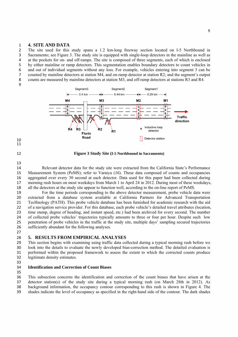
4. SITE AND DATA 1 The site used for this study spans a 1.2 km-long freeway section located on I-5 Northbound in 2 Sacramento; see Figure 3. The study site is equipped with single-loop detectors in the mainline as well as 3 at the pockets for on- and off-ramps. The site is composed of three segments, each of which is enclosed 4 by either mainline or ramp detectors. This segmentation enables boundary detectors to count vehicles in 5 and out of individual segments without any loss. For example, vehicles entering into segment 3 can be 6 counted by mainline detectors at station M4, and on-ramp detector at station R2; and the segment’s output 7 counts are measured by mainline detectors at station M3, and off-ramp detectors at stations R3 and R4. 8  9 

 10  11 

Figure 3 Study Site (I-5 Northbound in Sacramento) 12 

13 Relevant detector data for the study site were extracted from the California State’s Performance 14 

Measurement System (PeMS); refer to Varaiya (16). These data composed of counts and occupancies 15 aggregated over every 30 second at each detector. Data used for this paper had been collected during 16 morning rush hours on most weekdays from March 1 to April 24 in 2012. During most of these weekdays, 17 all the detectors at the study site appear to function well, according to the on-line report of PeMS. 18 

For the time periods corresponding to the above detector measurement, probe vehicle data were 19 extracted from a database system available at California Partners for Advanced Transportation 20 TecHnology (PATH). This probe vehicle database has been furnished for academic research with the aid 21 of a navigation service provider. For this database, each probe vehicle’s detailed travel attributes (location, 22 time stamp, degree of heading, and instant speed, etc.) had been archived for every second. The number 23 of collected probe vehicles’ trajectories typically amounts to three or four per hour. Despite such low 24 penetration of probe vehicles in the traffic at the study site, multiple days’ sampling secured trajectories 25 sufficiently abundant for the following analyses. 26  27 

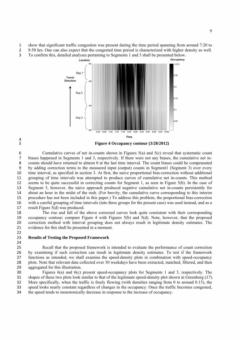
5. RESULTS FROM EMPIRICAL ANALYSES 28 This section begins with examining using traffic data collected during a typical morning rush before we 29 look into the details to evaluate the newly developed bias-correction method. The detailed evaluation is 30 performed within the proposed framework to assess the extent to which the corrected counts produce 31 legitimate density estimates. 32  33 Identification and Correction of Count Biases 34  35 This subsection concerns the identification and correction of the count biases that have arisen at the 36 detector station(s) of the study site during a typical morning rush (on March 28th in 2012). As 37 background information, the occupancy contour corresponding to this rush is shown in Figure 4. The 38 shades indicate the level of occupancy as specified in the right-hand side of the contour. The dark shades 39 

9  

  

show that significant traffic congestion was present during the time period spanning from around 7:20 to 1 8:50 hrs. One can also expect that the congested time period is characterized with higher density as well. 2 To confirm this, detailed analyses pertaining to Segments 1 and 3 shall be presented below. 3 

4  Figure 4 Occupancy contour (3/28/2012) 5 

Cumulative curves of net in-counts shown in Figures 5(a) and 5(c) reveal that systematic count 6 biases happened in Segments 1 and 3, respectively. If there were not any biases, the cumulative net in-7 counts should have returned to almost 0 at the last time interval. The count biases could be compensated 8 by adding correction terms to the measured input (output) counts in Segment1 (Segment 3) over every 9 time interval, as specified in section 3. At first, the naive proportional bias-correction without additional 10 grouping of time intervals was attempted to produce curves of cumulative net in-counts. This method 11 seems to be quite successful in correcting counts for Segment 1, as seen in Figure 5(b). In the case of 12 Segment 3, however, the naive approach produced negative cumulative net in-counts persistently for 13 about an hour in the midst of the rush. (For brevity, the cumulative curve corresponding to this interim 14 procedure has not been included in this paper.) To address this problem, the proportional bias-correction 15 with a careful grouping of time intervals (into three groups for the present case) was used instead, and as a 16 result Figure 5(d) was produced. 17  The rise and fall of the above corrected curves look quite consistent with their corresponding 18 occupancy contour; compare Figure 4 with Figures 5(b) and 5(d). Note, however, that the proposed 19 correction method with interval grouping does not always result in legitimate density estimates. The 20 evidence for this shall be presented in a moment. 21  22 Results of Testing the Proposed Framework 23  24  Recall that the proposed framework is intended to evaluate the performance of count correction 25 by examining if such correction can result in legitimate density estimates. To test if the framework 26 functions as intended, we shall examine the speed-density plots in combination with speed-occupancy 27 plots. Note that relevant data collected over 30 weekdays have been extracted, matched, filtered, and then 28 aggregated for this illustration. 29  Figures 6(a) and 6(c) present speed-occupancy plots for Segments 1 and 3, respectively. The 30 shapes of these two plots look similar to that of the legitimate speed-density plot shown in Greenberg (17). 31 More specifically, when the traffic is freely flowing (with densities ranging from 0 to around 0.15), the 32 speed looks nearly constant regardless of changes in the occupancy. Once the traffic becomes congested, 33 the speed tends to monotonically decrease in response to the increase of occupancy. 34 

10  

  

1  2 

(a) Cumulative curve of net in-counts into Segment 1 (uncorrected)

(b) Cumulative curve of net in-counts into Segment 1 (corrected)

(c) Cumulative curve of net in-counts into Segment 3 (uncorrected)

(d) Cumulative curve of net in-counts into Segment 3 (corrected)

(a) (b)

(c) (d)

Time Time

TimeTime

3  4 

5  Figure 5 Cumulative curves of net in-counts (3/28/2012) 6 

7 

11  

  

1 

Figure 6 Speed-Occupancy and Speed-Density plots 2 

3 

4 

12  

  

On the other hand, speed-density plots for Segments 1 and 3 are shown in Figures 6(b) and 6(d), 1 respectively. Recall that these two plots were constructed using density estimates corrected by the 2 proposed bias-correction approach. Figures 6(b) and 6(d) should have been well matched with Figures 6 3 (a) and 6 (c), respectively, considering that occupancy is the dimensionless measure of density, and that 4 measurement of occupancy and speed look quite reliable as seen in Figures 6 (a) and 6 (c). The data 5 points shown in Figures 6(b) and 6(d), however, reveal some illegitimate density values, as highlighted by 6 the three dotted ovals in the figures. 7  The above case study confirms the feasibility of applying the proposed framework to determine 8 qualitatively whether a bias-correction method performs well or not. In addition, we find that the tested 9 bias-correction approach in general appears to perform properly but it can produce spurious density 10 estimates on certain occasions. Note that applications of the proposed framework need not be confined to 11 the bias-correction approach tested here. 12 

13 

6. CONCLUSION 14 This paper proposes a new framework to evaluate the performance of bias-correction to vehicle counts 15 measured at freeway loop detectors. The evaluation of correcting count-biases has been performed by 16 inspecting the legitimacy of the density estimates obtained with corrected counts. The test outcome turns 17 out quite encouraging if we consider that the average penetration rate of probe vehicles used for the 18 present evaluation was quite low. 19 

A newly developed approach to correct count-biases in general performs properly. A detailed 20 investigation, however, reveals that the proposed bias-correction approach produces somewhat spurious 21 density estimates on certain occasions. We may suspect that such problematic occasions might happen 22 when some unknown factors play a role in significantly distorting the way count biases accumulates over 23 certain portion of the study period. Further investigations into such factors would be worthwhile. 24  For simplicity, this paper focused on the proposed bias-correction approach. As a further study, 25 however, other bias-correction methods can be tested using the proposed framework. Further, we may 26 consider testing the feasibility of employing the proposed framework for other applications such as 27 filtering out illegitimate density estimates on the hourly basis. Such a higher-resolution application would 28 be realized only when much more probe vehicles are penetrated into the traffic. 29  30 

ACKNOWLEDGMENTS 31  32 Thanks should be due to both Mr. Joseph Butler (California PATH) and Professor Alexandre Bayen 33 (University of California, Berkeley) for approving the access to the database of probe vehicles. 34  35 

36 REFERENCES 37 1. Nihan, N.L., 1997. Aid to determining freeway metering rates and detecting loop errors. Journal of 38 

Transportation Engineering 123, 454-458. 39 2. Jacobson, L.N., Nihan, N.L., Bender, J.D., 1990. Detecting erroneous loop detector data in a freeway 40 

traffic management system. Transportation Research Record 1287, 151-166. 41 3. Jia, Z., Chen, C., Coiffman, B., Varaiya, P., 2001. The PeMS algorithms for accurate, real-time 42 

estimates of g-factors and speeds from single-loop detectors, IEEE Intelligent Transportation Systems 43 Conference Proceedings, Oakland. 44 

4. Lee, H., Coiffman, B., 2012. Quantifying loop detector sensitivity and correcting detection problems 45 on freeways. Journal of Transportation Engineering 138, 871-881. 46 

5. Courage, K.G., Bauer, C.S., Ross, D.W., 1976. Operating parameters for main line sensors in freeway 47 surveillance systems. Transportation Research Record 601, 19-28. 48 

6. Payne, H.J., Thompson, S., 1997. Malfunction detection and data repair for induction-loop sensors 49 using I-880 data base. Transportation Research Record 1570, 191-201. 50 

13  

  

7. Petty, K., Noeimi, H., Sanwal, K., Rydzewski, D., Skabardonis, A., Varaiya, P., Al-deek, H., 1996. The 1 freeway service patrol evaluation project: Database support programs, and accessibility. 2 Transportation Research C 4, 71-85. 3 

8. Chen, L., May, A.D., 1987. Traffic detector errors and diagnostics. Transportation Research Record 4 1132, 82-93. 5 

9. Lee, H., Coiffman, B., 2012. Identifying chronic splashover errors at freeway loop detectors. 6 Transportation Research Part C 24, 141-156. 7 

10. Turochy, R.E., Smith, B.L., 2000. New procedure for detector data screening in traffic management 8 systems. Transportation Research Record 1727, 127-131. 9 

11. Chen, C., Kwon, J., Rice, J., Skabardonis, A., Varaiya, P., 2003. Detecting errors and imputing 10 missing data for single-loop surveillance systems. Transportation Research Record 1855, 160-167. 11 

12. Wall, Z.R., Dailey, D.J., 2003. Algorithm for detecting and correcting errors in archived traffic data. 12 Transportation Research Record 1855, 183-190. 13 

13. Vanajakshi, L., Rilett, L.R., 2004. Loop detector data diagnostics based on conservation-of-vehicles 14 principle. Transportation Research Record 1870, 162-169. 15 

14. Kurada, L., Öğüt, K.S., Banks, J.H., 2007. Evaluation of N-curve methodology for analysis of 16 complex bottlenecks. Transportation Research Record 1999, 54-61. 17 

15. Edie, L.C. 1965. Discussion of traffic stream measurements and definitions. Proceedings of the 18 Second International Symposium on the Theory of Traffic Flow. J. Almond (Editor), Paris, OECD: 19 139-154 20 

16. Varaiya, P., 2009. The Freeway Performance Measurement System (PeMS), PeMS 9.0: Final Report. 21 Institute of Transportation Studies, Berkeley. 22 

17. Greenberg, H., 1959. An analysis of traffic flow. Operations Research 7, 79-85. 23