A General Procedure to Assess the Internal Structure of a Noncognitive Measure— The Student360 Insight Program (S360) Time Management Scale

Guangming Ling

Frank Rijmen

October 2011

Research Report ETS RR–11-42

October 2011

A General Procedure to Assess the Internal Structure of a Noncognitive Measure—

The Student360 Insight Program (S360) Time Management Scale

Guangming Ling and Frank Rijmen

ETS, Princeton, New Jersey

Technical Review Editor: Dan Eignor

Technical Reviewers: Don Powers and Yigal Attali

Copyright © 2011 by Educational Testing Service. All rights reserved.

ETS, the ETS logo, and LISTENING. LEARNING. LEADING., are registered trademarks of Educational Testing Service (ETS).

As part of its nonprofit mission, ETS conducts and disseminates the results of research to advance

quality and equity in education and assessment for the benefit of ETS’s constituents and the field.

To obtain a PDF or a print copy of a report, please visit:

http://www.ets.org/research/contact.html

i

Abstract

The factorial structure of the Time Management (TM) scale of the Student 360: Insight Program

(S360) was evaluated based on a national sample. A general procedure with a variety of methods

was introduced and implemented, including the computation of descriptive statistics, exploratory

factor analysis (EFA), and confirmatory factor analysis (CFA). Overall, the results indicated that

the TM scale measured multidimensional constructs of TM with 5 factors. The paper concludes

with a discussion of several issues concerning the wording of items and residual dependencies,

as well as future directions for research.

Key words: factorial structure, time management exploratory factor analysis, confirmatory factor

analysis, residual dependence

ii

Acknowledgments

This paper benefited from discussions with Ou (Lydia) Liu, Richard Roberts, and Brent

Bridgeman. The authors thank Jonathan Steinberg for his support in preparing the data.

iii

Table of Contents

Page

Background ..................................................................................................................................... 1

Method ............................................................................................................................................ 2

Results ............................................................................................................................................. 3

Descriptive Analyses ............................................................................................................... 3

Exploratory Factor Analysis .................................................................................................. 10

Confirmatory Factor Analysis (CFA) .................................................................................... 16

Summary and Discussion .............................................................................................................. 20

References ..................................................................................................................................... 24

List of Appendices ........................................................................................................................ 27

iv

List of Tables

Page

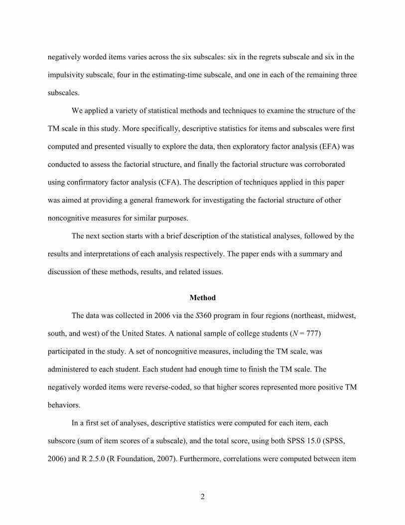
Table 1. Descriptive Statistics for Each of the Six Subscales ..................................................... 5

Table 2. Average Inter-Item Correlations Within Each Subscale and the Total Test ................. 8

Table 3. Correlations Among Subscale Scores ......................................................................... 10

Table 4. Factor Loadings of the 36 Items (4-, 5-, and 6-Factor Based on Polychoric

Correlations) ........................................................................................................... 12

Table 5. Exploratory Factor Analysis (EFA) of the Factorial Structure of the Six Subscale

Scores ..................................................................................................................... 16

Table 6. Model Fit Indices for the Measurement Model of Each Subscale (Polychoric and

Weighted Least Square [WLS]) ............................................................................. 19

v

List of Figures

Page

Figure 1. Bar plots of the 36 items. Each row represents one subscale. An * indicates that the

item was negatively worded and reverse-coded. .......................................................... 5

Figure 2. Colored correlation matrices for Pearson (below the diagonal) and polychoric (above

the diagonal) correlations. ............................................................................................. 7

Figure 3. Screeplot of the eigenvalues of the polychoric correlation matrix of the 36 items. ...... 11

1

Background

The Student360: Insight Program (S360) is a Web-based source of self-help tools

intended to assist students—particularly those who are attending or preparing to attend

community college—in planning and meeting their college objectives. The program includes a

set of surveys and assessments, focused feedback, interventions, and tutorials. A set of

noncognitive constructs are assessed by the S360, including study skills, time management (TM),

test anxiety, interests, and teamwork. The current study focuses on the TM scale.

Over the last three decades, quite a few TM scales have been developed, such as the time

management behavior scale (TMBS; Macan, Shahani, Dipboye, & Philips, 1990), the time

structure questionnaire (TSQ; Bond & Feather, 1988), and the time management questionnaire

(TMQ; Britton & Tesser, 1991). These scales were typically developed and investigated in the

areas of industrial and organizational psychology and management. These scales carry the

following concern: When the factorial structure of each of these TM scales was studied, the

sample size employed was small. The current version of the TM scale comes from an extension

of the Australian time organization management scale (ATOMS; Roberts, Krause, & Suk-Lee,

2001), adopting a definition of TM suggested by Lankein (1973). Six subscales were originally

developed: the persistence subscale (perseverance to finish tasks and schedules), the estimating-

time subscale (time estimation related to completing tasks), the calendar subscale (mechanism of

TM), the regrets subscale (coping with time), the impulsivity subscale (preference for planning),

and the clean-desk subscale (effective organization). Each subscale is measured by six items

about specific TM behaviors. The test-takers are required to rate how well the description in the

item matches his or her behavior on a Likert scale from 1 (disagree) to 4 (strongly agree).

Nineteen items are negatively worded, meaning that negatively connoted or inefficient TM

behaviors are described (see Appendix A for the six subscales and items). The number of

2

negatively worded items varies across the six subscales: six in the regrets subscale and six in the

impulsivity subscale, four in the estimating-time subscale, and one in each of the remaining three

subscales.

We applied a variety of statistical methods and techniques to examine the structure of the

TM scale in this study. More specifically, descriptive statistics for items and subscales were first

computed and presented visually to explore the data, then exploratory factor analysis (EFA) was

conducted to assess the factorial structure, and finally the factorial structure was corroborated

using confirmatory factor analysis (CFA). The description of techniques applied in this paper

was aimed at providing a general framework for investigating the factorial structure of other

noncognitive measures for similar purposes.

The next section starts with a brief description of the statistical analyses, followed by the

results and interpretations of each analysis respectively. The paper ends with a summary and

discussion of these methods, results, and related issues.

Method

The data was collected in 2006 via the S360 program in four regions (northeast, midwest,

south, and west) of the United States. A national sample of college students (N = 777)

participated in the study. A set of noncognitive measures, including the TM scale, was

administered to each student. Each student had enough time to finish the TM scale. The

negatively worded items were reverse-coded, so that higher scores represented more positive TM

behaviors.

In a first set of analyses, descriptive statistics were computed for each item, each

subscore (sum of item scores of a subscale), and the total score, using both SPSS 15.0 (SPSS,

2006) and R 2.5.0 (R Foundation, 2007). Furthermore, correlations were computed between item

3

scores, between subscores, and between each subscore and the total score. An interitem

correlation matrix was created based on the data, as well as an intersubscale correlation matrix.

The interitem correlation matrix was represented visually in a chart. More specifically, darker

colors were assigned to greater values of correlation in the matrix. Reliability analyses for each

subscale and the total test were also performed.

In a second set of analyses, exploratory factor analyses were conducted based on the

interitem correlation matrix and intersubscore correlation matrix separately. Parallel analysis was

applied to determine the number of factors using both SPSS 15.0 and SAS 9.1 (Fabrigar, Wegener,

MacCallum, & Strahan, 1999; Horn, 1965; SAS, 2004; SPSS, 2006).

Finally, several waves of CFA were conducted using LISREL 8.8 (Jöreskog & Sörbom,

2001) to test whether the identified underlying factorial structure represented the data

adequately. The confirmatory models were inspired by the internal structure defined by the test

developers, as well as by the results of the exploratory factor analysis. In addition, several other

structural equation models with higher-order factors were tested and compared.

Results

Descriptive Analyses

Among all the participants, 443 (57%) were female students and 334 were male

students; about 46% were Caucasian, 18% were African American, 21% were Hispanic, 7%

were Asian American, and the remaining were students from other ethnic groups. The average

age of the sample was 23.62 years (SD = 8.84), and 90% of the students were in the range of 16

to 40 years old.

The number of missing responses per item ranged from 0 to 3 (0% to 0.4% in terms of

percentage) across the 36 items; the average percentage of missing responses across items was

4

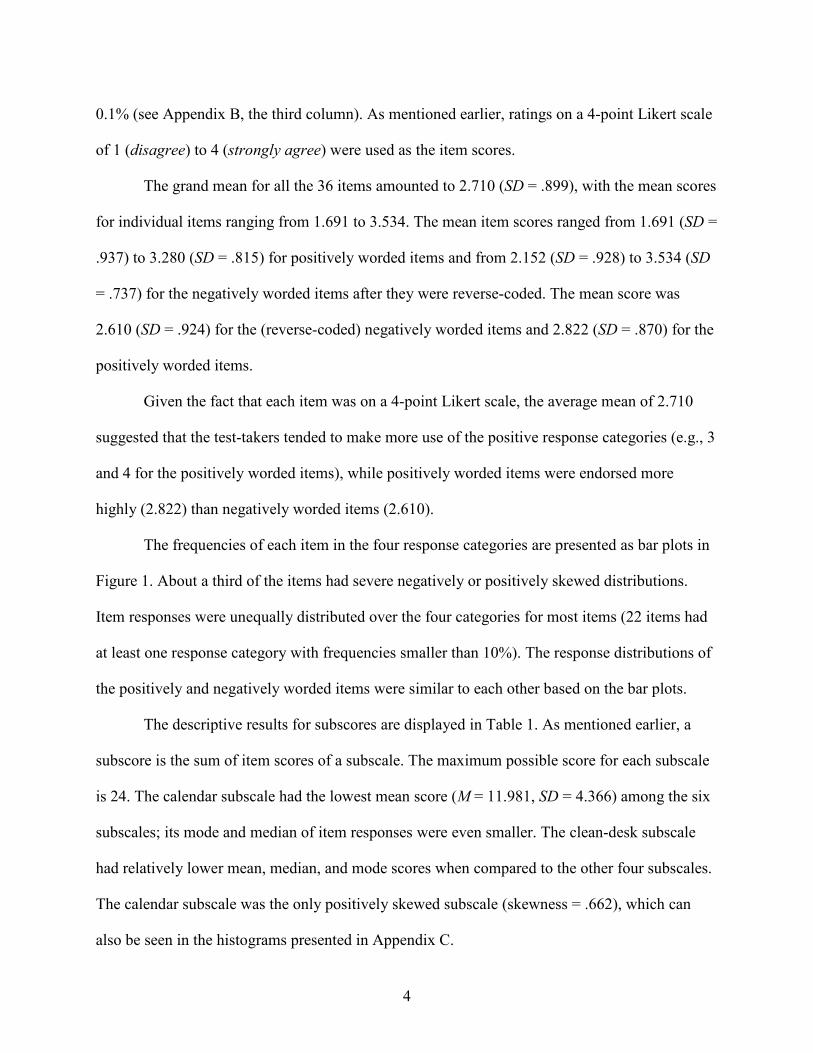
0.1% (see Appendix B, the third column). As mentioned earlier, ratings on a 4-point Likert scale

of 1 (disagree) to 4 (strongly agree) were used as the item scores.

The grand mean for all the 36 items amounted to 2.710 (SD = .899), with the mean scores

for individual items ranging from 1.691 to 3.534. The mean item scores ranged from 1.691 (SD =

.937) to 3.280 (SD = .815) for positively worded items and from 2.152 (SD = .928) to 3.534 (SD

= .737) for the negatively worded items after they were reverse-coded. The mean score was

2.610 (SD = .924) for the (reverse-coded) negatively worded items and 2.822 (SD = .870) for the

positively worded items.

Given the fact that each item was on a 4-point Likert scale, the average mean of 2.710

suggested that the test-takers tended to make more use of the positive response categories (e.g., 3

and 4 for the positively worded items), while positively worded items were endorsed more

highly (2.822) than negatively worded items (2.610).

The frequencies of each item in the four response categories are presented as bar plots in

Figure 1. About a third of the items had severe negatively or positively skewed distributions.

Item responses were unequally distributed over the four categories for most items (22 items had

at least one response category with frequencies smaller than 10%). The response distributions of

the positively and negatively worded items were similar to each other based on the bar plots.

The descriptive results for subscores are displayed in Table 1. As mentioned earlier, a

subscore is the sum of item scores of a subscale. The maximum possible score for each subscale

is 24. The calendar subscale had the lowest mean score (M = 11.981, SD = 4.366) among the six

subscales; its mode and median of item responses were even smaller. The clean-desk subscale

had relatively lower mean, median, and mode scores when compared to the other four subscales.

The calendar subscale was the only positively skewed subscale (skewness = .662), which can

also be seen in the histograms presented in Appendix C.

5

Figure 1. Bar plots of the 36 items. Each row represents one subscale. An * indicates that

the item was negatively worded and reverse-coded.

Table 1

Descriptive Statistics for Each of the Six Subscales

Subscales N # missing M Median Mode SD Skewness Kurtosis

Persistence 772 5 18.488 19 20 3.171 -.289 -.491 Estimating-time 775 2 16.861 17 17 3.283 -.120 -.383 Calendar 774 3 11.981 11 7 4.366 .662 -.217 Regrets 773 4 17.157 18 18 3.279 -.653 .481 Impulsivity 766 11 16.841 17 17 3.543 -.443 030 Clean-desk 770 7 16.222 16 14 4.076 -.005 -.542

S1

S2

S3

S4

S5

S6

6

For exploratory purposes, both Pearson correlations and polychoric correlations between

item scores were computed and compared. Researchers in social science and psychological

science often treat the Likert-scaled item responses or ratings (with the TM scale where 1 to 4

represents disagree to strongly agree) as if it were on an interval scale, assuming a normally

distributed latent variable underlies it (Olsson, 1979; Wainer & Thissen, 1976). The Pearson

correlations among these item scores/ratings are then obtained as the estimates of correlations

among these underlying variables. However, the Pearson correlations of ordinal/Likert-scaled

responses may underestimate the correlations between the latent variables underlying them

(Jöreskog & Sörbom, 1988, p.10–12; Olsson, 1979). In such cases, the polychoric correlations

are typically preferred over the Pearson correlations, especially when the items have heavily

skewed distributions. When the Likert-scaled responses to individual items are not too severely

deviated from a normal distribution, the Pearson correlation estimation is acceptably robust

(Olsson, 1979). Given the fact that a third of items of the TM scale had severely skewed

distributions, we decided to use the polychoric correlation as the measure of association in this

study in addition to the Pearson correlation.

The Pearson and polychoric correlation matrices were computed in PRELIS 2 (Jöreskog

& Sörbom, 1988) and are visually represented in Figure 2. The Pearson correlations were

computed over all cases that had valid values on both variables (i.e., pairwise deletion was

employed). The lower triangle of this matrix (below the diagonal) presents the Pearson

correlations, and the upper triangle (above the diagonal) presents the polychoric correlations. The

cells with a darker color represent a stronger interitem association in Figure 2.

In general, the two types of correlations shared similar patterns of interitem associations,

except that the polychoric correlations were slightly higher (in darker colors in Figure 2) than the

Pearson correlations in general, as was suggested by Olsson (1979) and Jöreskog & Sörbom

7

(1988). The correlations between items within the same subscale were generally higher (cells in

darker colors in Figure 2) than the correlations of items from different subscales. However,

moderate levels of correlations were also found between some items from different subscales

(e.g., between items from the persistence subscale and the estimating-time subscale, and between

items from the regrets subscale and the impulsivity subscale; see Figure 2). These cross-subscale

interitem correlations indicated that a certain level of association exists among the subscales.

Figure 2. Colored correlation matrices for Pearson (below the diagonal) and polychoric

(above the diagonal) correlations.

8

The average value of the interitem polychoric correlations of all 36 items was .16, and the

average within-subscale interitem polychoric correlations ranged from .33 (the estimating-time

subscale) to .53 (the calendar subscale, see Table 2). The within-subscale interitem correlation on

average was higher than the overall average interitem correlations.

Further inspection revealed that the higher within-subscale average interitem correlation

was not due to extreme values of single item pairs. For example, the 15 interitem polychoric

correlations for the calendar subscale were all greater than .40, which was much higher than .16

(the average interitem polychoric correlations over all items). Similar results were found for the

other subscales except for the estimating-time subscale, where there were two interitem polychoric

correlations lower than .16. Similar results were found based on the Pearson correlations.

In summary, the patterns found in the colored correlation matrix suggest that several

dimensions might be present in the current data. The calendar subscale and the clean-desk

subscale seem to be distinct from the other subscales, while the persistence subscale and the

estimating-time subscale seem to mix with each other and measure a common factor. The regrets

subscale and the impulsivity subscale also seem to measure something in common, but to a

Table 2

Average Inter-Item Correlations Within Each Subscale and the Total Test

Subscale Range of interitem polychoric correlations

Average interitem polychoric correlation

Cronbach’s Alpha

Persistence .09 ~ .44 .37 .715 Estimating-time .06 ~ .54 .33 .698 Calendar .31 ~ .62 .53 .828 Regrets .15 ~ .65 .35 .716 Impulsivity .17 ~ .47 .39 .750 Clean-desk .17 ~ .59 .44 .782 Total test -.24 ~ .65 .16 .842

9

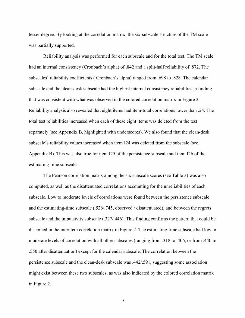
lesser degree. By looking at the correlation matrix, the six-subscale structure of the TM scale

was partially supported.

Reliability analysis was performed for each subscale and for the total test. The TM scale

had an internal consistency (Cronbach’s alpha) of .842 and a split-half reliability of .872. The

subscales’ reliability coefficients ( Cronbach’s alpha) ranged from .698 to .828. The calendar

subscale and the clean-desk subscale had the highest internal consistency reliabilities, a finding

that was consistent with what was observed in the colored correlation matrix in Figure 2.

Reliability analysis also revealed that eight items had item-total correlations lower than .24. The

total test reliabilities increased when each of these eight items was deleted from the test

separately (see Appendix B, highlighted with underscores). We also found that the clean-desk

subscale’s reliability values increased when item I24 was deleted from the subscale (see

Appendix B). This was also true for item I25 of the persistence subscale and item I26 of the

estimating-time subscale.

The Pearson correlation matrix among the six subscale scores (see Table 3) was also

computed, as well as the disattenuated correlations accounting for the unreliabilities of each

subscale. Low to moderate levels of correlations were found between the persistence subscale

and the estimating-time subscale (.526/.745, observed / disattenuated), and between the regrets

subscale and the impulsivity subscale (.327/.446). This finding confirms the pattern that could be

discerned in the interitem correlation matrix in Figure 2. The estimating-time subscale had low to

moderate levels of correlation with all other subscales (ranging from .318 to .406, or from .440 to

.550 after disattenuation) except for the calendar subscale. The correlation between the

persistence subscale and the clean-desk subscale was .442/.591, suggesting some association

might exist between these two subscales, as was also indicated by the colored correlation matrix

in Figure 2.

10

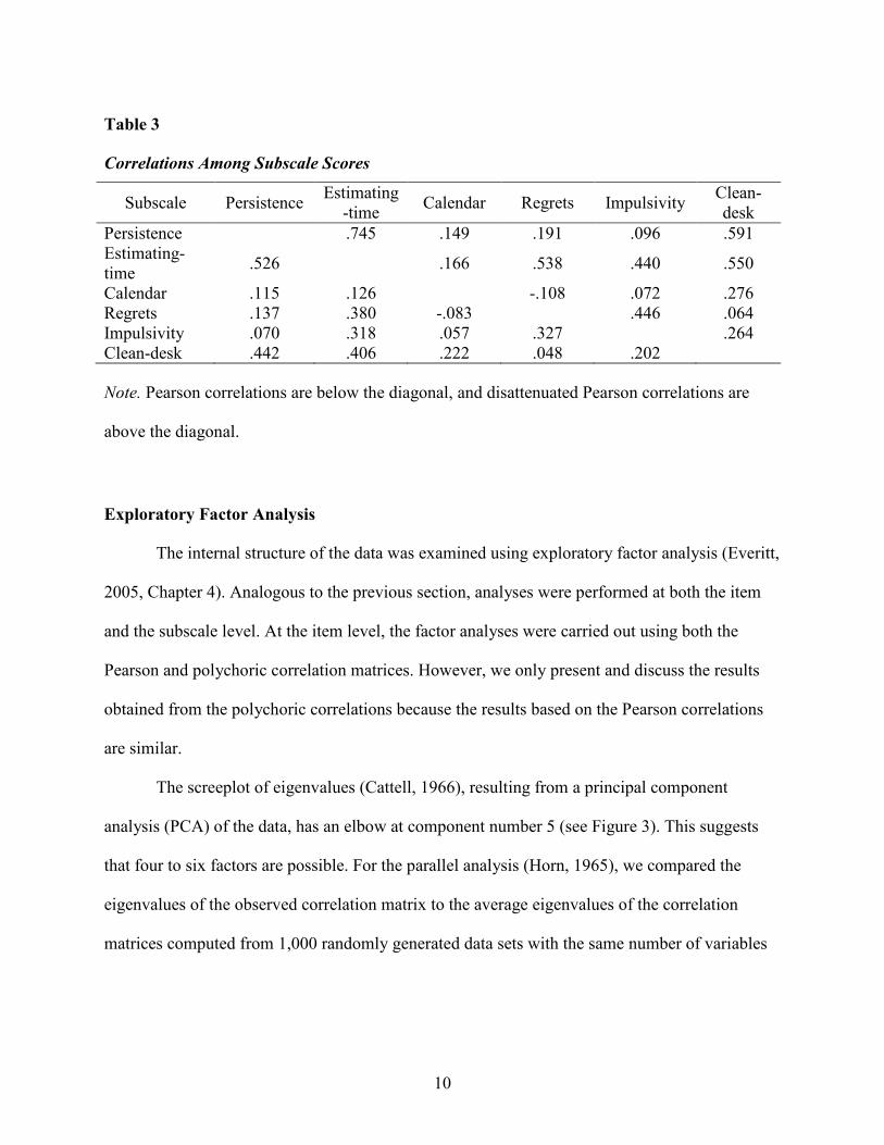
Table 3

Correlations Among Subscale Scores

Subscale Persistence Estimating-time Calendar Regrets Impulsivity Clean-

desk Persistence .745 .149 .191 .096 .591 Estimating-time .526 .166 .538 .440 .550

Calendar .115 .126 -.108 .072 .276 Regrets .137 .380 -.083 .446 .064 Impulsivity .070 .318 .057 .327 .264 Clean-desk .442 .406 .222 .048 .202

Note. Pearson correlations are below the diagonal, and disattenuated Pearson correlations are

above the diagonal.

Exploratory Factor Analysis

The internal structure of the data was examined using exploratory factor analysis (Everitt,

2005, Chapter 4). Analogous to the previous section, analyses were performed at both the item

and the subscale level. At the item level, the factor analyses were carried out using both the

Pearson and polychoric correlation matrices. However, we only present and discuss the results

obtained from the polychoric correlations because the results based on the Pearson correlations

are similar.

The screeplot of eigenvalues (Cattell, 1966), resulting from a principal component

analysis (PCA) of the data, has an elbow at component number 5 (see Figure 3). This suggests

that four to six factors are possible. For the parallel analysis (Horn, 1965), we compared the

eigenvalues of the observed correlation matrix to the average eigenvalues of the correlation

matrices computed from 1,000 randomly generated data sets with the same number of variables

11

Figure 3. Screeplot of the eigenvalues of the polychoric correlation matrix of the 36 items.

Note. The squares are results of the average eigenvalues determined from the parallel analysis.

and the same sample size. It was found that the two sets of eigenvalues overlapped between the

factor numbers of 4 and 5. We decided to analyze the 4- and 5-factor models in the next step, as

was recommended by O’Connor (2000). In addition, we also examined a 6-factor structure since

it was prespecified by the test developers.

The exploratory factor analyses were carried out using the maximum likelihood

estimation method and Promax rotation (Hendrickson & White, 1964). As noted above, solutions

were obtained for four, five, and six factors. The factor loadings of the 36 items for the 4-, 5-,

and 6-factor solution based on the polychoric correlations are displayed in Table 4, where

loadings less than .3 are omitted (Comrey & Lee, 1992; Costello & Osborne, 2005) and items

belonging to the same subscale predefined by assessment developers are presented together in a

block. Negatively worded items are marked in Table 4.

12

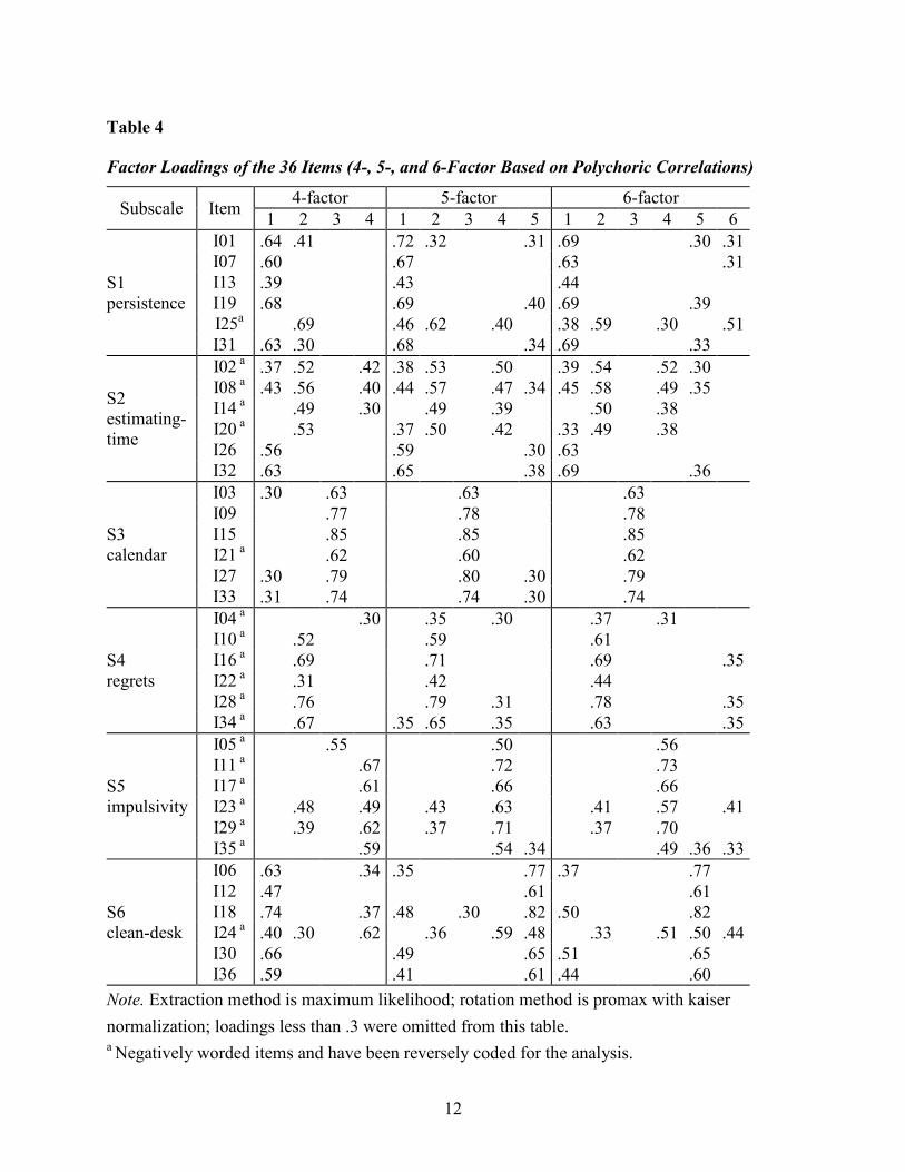
Table 4

Factor Loadings of the 36 Items (4-, 5-, and 6-Factor Based on Polychoric Correlations)

Subscale Item 4-factor 5-factor 6-factor 1 2 3 4 1 2 3 4 5 1 2 3 4 5 6

S1 persistence

I01 .64 .41 .72 .32 .31 .69 .30 .31 I07 .60 .67 .63 .31 I13 .39 .43 .44 I19 .68 .69 .40 .69 .39

I25a .69 .46 .62 .40 .38 .59 .30 .51 I31 .63 .30 .68 .34 .69 .33

S2 estimating- time

I02 a .37 .52 .42 .38 .53 .50 .39 .54 .52 .30 I08 a .43 .56 .40 .44 .57 .47 .34 .45 .58 .49 .35 I14 a .49 .30 .49 .39 .50 .38 I20 a .53 .37 .50 .42 .33 .49 .38 I26 .56 .59 .30 .63 I32 .63 .65 .38 .69 .36

S3 calendar

I03 .30 .63 .63 .63 I09 .77 .78 .78 I15 .85 .85 .85

I21 a .62 .60 .62 I27 .30 .79 .80 .30 .79 I33 .31 .74 .74 .30 .74

S4 regrets

I04 a .30 .35 .30 .37 .31 I10 a .52 .59 .61 I16 a .69 .71 .69 .35 I22 a .31 .42 .44 I28 a .76 .79 .31 .78 .35 I34 a .67 .35 .65 .35 .63 .35

S5 impulsivity

I05 a .55 .50 .56 I11 a .67 .72 .73 I17 a .61 .66 .66 I23 a .48 .49 .43 .63 .41 .57 .41 I29 a .39 .62 .37 .71 .37 .70 I35 a .59 .54 .34 .49 .36 .33

S6 clean-desk

I06 .63 .34 .35 .77 .37 .77 I12 .47 .61 .61 I18 .74 .37 .48 .30 .82 .50 .82

I24 a .40 .30 .62 .36 .59 .48 .33 .51 .50 .44 I30 .66 .49 .65 .51 .65 I36 .59 .41 .61 .44 .60

Note. Extraction method is maximum likelihood; rotation method is promax with kaiser normalization; loadings less than .3 were omitted from this table. a Negatively worded items and have been reversely coded for the analysis.

13

In the 4-factor structure, the first factor had 18 items with substantial loadings. More

specifically, six items were from the clean-desk subscale; five items were from the persistence

subscale; and four items were from the estimating-time subscale (see Table 4). All items loading

on this factor were positively worded items, except for item I24 from the clean-desk subscale and

items I02 and I08 from the estimating-time subscale. The second factor had 15 items with

substantial loadings, mainly from the estimating-time subscale (4 items) and the regrets subscale

(5 items). All of the items with substantial loadings on the second factor were negatively worded

items, except for two items from the persistence subscale (I01 and I31).

The third factor seemed to be very unique among the other factors. The items with

substantial loadings on this factor were exclusively from the calendar subscale except for item

I05 (see Table 4). It should be noted that three items of the calendar subscale also had substantial

loadings on the first factor. The fourth factor had 12 items with a substantial loading on it,

predominantly from the impulsivity subscale (5 items), the estimating-time subscale (3 items),

and the clean-desk subscale (3 items). Most of these items were negatively worded.

The six items of the estimating-time subscale loaded on multiple factors. The four

negatively worded items substantially loaded on the second factor, while the two positively

worded items only loaded on the first factor. Among the four negatively worded items, three of

them also had substantial loadings on the fourth factor, and two also loaded on the first factor

substantially (see Table 4).

In the 5-factor solution, the item-factor loading pattern was similar to that of the 4-factor

solution, except that all six items from the clean-desk subscale now loaded substantially on the

fifth factor, with four items loading substantially on the first fact as well.

14

The exploratory results for the 6-factor solution were not so different from the results of

the 5-factor solution. Nine items had substantial loadings on the sixth factor, but all of them had

substantial loadings on one or more of the other factors.

Some items did not have a substantial loading on the same factor that was loaded on by

the other items from the same subscale. For example, item I04 in the regrets subscale loaded

lower than .3 on the second factor while the other items of this subscale had loadings higher than

.3 on the same factor (see the 4-factor solution in Table 4). This pattern was the same for the 4-,

5-, and 6-factor solution. Item I04 asks, “I think about the road not taken,” which might not

necessarily be related to regret in the context of TM behaviors, and hence may be different from

the other items of that subscale. In the persistence subscale, item I25 did not load on the same

factor as the other items did (in the 4- and 6-factor structure) and had a cross-loading on other

factors (in the 5-factor structure). The item describes: “I give up when the ‘going gets tough.’”

The colloquial term “going gets tough” may have been unclear to some of the participants.

The exploratory factor analysis results partially supported the structure predefined by the

test developers. The calendar subscale and the regrets subscale appeared in the exploratory

analysis as each loaded on a separate factor very well. The impulsivity subscale, the clean-desk

subscale, and the persistence subscale also showed up as distinctive factors in the EFA.

However, some items of these subscales had different loadings than the other items of the

subscale on a particular factor or had a substantial loading on factors different from the other

items of the subscale. The estimating-time subscale did not emerge with a clear loading pattern.

The six items loaded on different factors, with the two positively worded items always loading

on a factor different from the negatively worded items. Furthermore, the persistence subscale and

the clean-desk subscale primarily loaded on the same factor.

15

In summary, two models were obtained from the item level EFA: the 4-factor model and

the 5-factor model. In the 4-factor solution, the predefined calendar subscale and the impulsivity

subscale each constituted a separate factor. A combination of the estimating-time subscale and

the regrets subscale formed the third factor. And a combination of the persistence subscale and

the clean-desk subscale formed the fourth factor. In the 5-factor structure, the regrets subscale

and the estimating-time subscale were combined into one factor, and the other four subscales

each appeared as a separate factor. The 6-factor model found in the EFA was not considered

given that the items with substantial loadings on the sixth factor was scattered around the six

subscales and made it hard to interpret.

An EFA was also performed based on the correlation matrix among the six subscale

scores. Mardia’s statistic was computed using PRELIS 2, the coefficient was .9266 (<3),

indicating an acceptable multivariate normality condition was met for the six subscale scores

(Jöreskog & Sörbom, 1988; Mardia, 1970). Parallel analysis indicated that there were two or

three factors underlying the six subscale scores. (See Appendix H for the screeplot.) Table 5

presented the subscale-factor loadings after Promax rotation based on an exploratory factor

analysis using the maximum likelihood estimation method. In both 2-factor and 3-factor models,

the persistence, the estimating-time, and the clean-desk subscales loaded on the first factor, while

the regrets and the impulsivity subscales, together with the persistence and the estimating-time

subscales, loaded on the second factor. The calendar subscale loaded on the third factor in the

3-factor model, together with the persistence, estimating-time, and clean-desk subscales. The

loading patterns between subscales and factors were not clear for both models and were difficult

to interpret. We decided not to employ CFA on these two factor models. However, the low

between-factor correlations (e.g., .22 for the 2-factor model) indicated that a multidimensional

structure is present in the TM scale.

16

Table 5

Exploratory Factor Analysis (EFA) of the Factorial Structure of the Six Subscale Scores

Subscale Factor 1 of 2 Factor 2 of 2 Factor 1 of 3 Factor 2 of 3 Factor 3 of 3

Persistence .70 .35 .99 .31 .49 Estimating-time .73 .66 .59 .63 .51 Calendar .35 Regrets .74 .73 Impulsivity .44 .50 Clean-desk .63 .48 .69

Note. Extraction method is maximum likelihood; rotation method is promax with kaiser

normalization. Factor loadings lower than .3 are omitted.

Confirmatory Factor Analysis (CFA)

Since the TM scale consisted of six subscales defined by the assessment developers, a

CFA was performed to evaluate whether a measurement model fit the data for each subscale

before fitting the models resulted from the EFA. A measurement model is a single factor model

where all indicators (items) load on the single factor and all the indicators’ residuals are

independent from each other (residuals’ covariances were all set as zero; see Raykov &

Marcoulidies, 2000). The measurement model was fitted to the polychoric correlation matrix of

items for each subscale separately (see Appendix E). The polychoric correlation was considered

instead of the Pearson correlations because more than a third of the items were heavily skewed

and the Pearson correlations might lead to a biased estimation of the interitem associations, as

mentioned in the previous section.

The polychoric correlations were estimated based on the asymptotically distribution free

(ADF) method (Browne, 1984), where a large sample size is generally required to estimate the

asymptotic covariance matrix for the polychoric correlations (Jöreskog & Sörbom, 2001, p. 59;

Bentler & Chou, 1987, p. 173). The asymptotic covariance matrix is typically analyzed with the

17

(diagonal) weighted least square estimation method. A weight matrix is obtained as the inverse

of the asymptotic covariance matrix, which then is used in the weighted least square (WLS,

using the full weight matrix), and the diagonal weighted least square (DWLS) estimation method

(using only the diagonal elements of the weight matrix). The DWLS is preferred when the

sample size is small or medium (Aish & Jöreskog, 1990; Jöreskog & Sörbom, 2001; Muthén,

1983) relative to the number of items and parameters.

In this study, the WLS estimation method was used to fit the factor models for individual

subscales and the DWLS estimation method was used to fit the factor models of the total test.

For each subscale, a measurement model with one latent trait measured by the six items

was fitted to the data using the WLS) estimation method. According to Browne & Cudeck (1993;

see also Hu & Bentler, 1999; Raykov & Marcoulidies, 2000; Yu & Muthén, 2001), a model with

the root mean square error approximate (RMSEA) value below .08 and the Tucker-Lewis index

(TLI, or comparative fit index [CFI]) value above .90 can be considered an acceptable fit; a

model with the RMSEA value below .05 and the TLI (and CFI) value above .95 can be

considered a good fit. Following these suggestions, four of the six subscales each had a good or

acceptable fit with the measurement model, the RMSEA values ranging from .009 to .068, and

the TLI values ranging from .94 to .99 (see Table 6). These good fit indices suggest that a

measurement model fitted the data well for these four subscales and a unidimensional latent

construct was measured by each of these four subscales.

The measurement model for the estimating-time subscale fitted poorly (RMSEA=.108,

TLI =.79, and CFI=.88; see Appendix E). The impulsivity subscale also had a poor model-data

fit (RMSEA=.118, TLI=.84, and CFI=.90). The modification indices (Raykov & Marcoulidies,

2000) for the covariances between errors for several items from these two subscales were found

to be very high. For the estimating-time subscale, the model fit would be improved with a Chi-

18

square change of 78.61 if releasing the error covariance between items I26 and I32 (all the error

covariances were fixed as zero in the measurement model). For the impulsivity subscale, the Chi-

square would change by 81.95 upon releasing the residual covariances between items I16 and

I28, and between items I22 and I34 (see Appendix E). The poor fit indices of these two

subscales, as well as the large Chi-square change indicated by the modification indices,

suggested that a measurement model did not fit the data well and some modifications might be

made to account for the non-zero residual covariances.

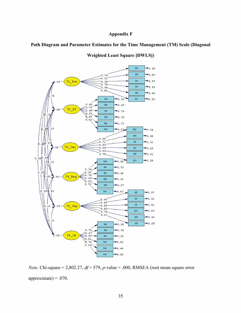
A more complete structural equation model with six hypothetical factors was then fit to

the polychoric correlation matrix of all 36 items, with a latent factor specified to be measured by

each subscale. No restrictions were imposed on the correlations between factors. (See Appendix

F for the path diagram of the model.) The model was estimated using DWLS. The fit statistics

were acceptable, with the RMSEA value of .070, the CFI value of .92, and the TLI value of .91

(see Table 6).

Furthermore, two confirmatory models based on the exploratory analysis results (the 4-

and 5-factor models in Table 4) were fit to the data. Recall that the 4-factor model was formed

by combining items of the estimating-time subscale and the regrets subscale to measure a single

factor, combining items of the persistence subscale and the clean-desk subscale to measure

another single factor, and keeping the remaining two subscales as two single factors. The 4-

factor model fit the data marginally well using the DWLS estimation method, with the RMSEA

value of .081, the TLI value of .88, and the CFI value of .89 (see Table 6 and Appendix G).

Better fit indices were obtained for the 5-factor model (combining items of the estimating-time

subscale and the regrets subscale to measure one single factor, with the remaining four subscales

as four single factors), with the RMSEA value of .062, the TLI value of .93, and the CFI value of

19

Table 6

Model Fit Indices for the Measurement Model of Each Subscale (Polychoric and Weighted

Least Square [WLS])

Subscale RMSEA TLI(NNFI) CFI Chi-square

Persistence .060 .94 .96 34.06 (df = 9)

Estimating-time .108 .79 .88 90.75 (df = 9)

Calendar .068 .96 .98 41.53 (df = 9)

Regrets .118 .84 .90 106.81 (df = 9)

Impulsivity .058 .94 .96 32.18 (df = 9)

Clean-desk 009 1.00 1.00 9.51 (df = 9)

Total test 6f (DWLS estimation) .070 .91 .92 2802.27 (df = 579)

Total test 4f (DWLS estimation) .081 .88 .89 3595.72 (df = 588)

Total test 5f (DWLS estimation) 062 .93 .94 2335.49 (df = 584)

Note. RMSEA = root mean square error approximate, TLI = Tucker-Lewis index, CFI =

comparative fit index, DWLS = diagonal weighted least square.

.94 (see Table 6 and Appendix H). The fit indices suggested that the 5-factor solution provided a

better balance between model-fit and model-complexity than the 6-factor model.

In addition to these models, a measurement model for all 36 items was also tested against

the data to examine whether a single factor underlies the 36 items. Two higher-order factor

models, one based on the 5-factor model and the other on the 6-factor model, were also tested

given the data. The higher-order factor models were tested to see whether a common latent

variable was present underlying the five or six factors, which could provide useful information

for the decisions of score reporting.

The measurement model did not converge, while the two higher-order factor models both

had poor model fit indices. The nonconvergence and poorly fitted higher-order models suggested

20

that the TM scale was not unidimensional, and it might not be a legitimate practice to report a

single total score for the TM scale. These results also confirmed the multidimensionality of the

TM scale inferred from the subscore-based EFA.

In summary, the CFA suggested that four of the six subscales each measured a

unidimensional construct separately. The other two subscales (the estimating-time subscale and

the impulsivity subscale) resulted in lack of fit due to the local dependencies among items. The

measurement model with all 36 items of the TM scale did not converge given the data. The two

higher-order factor models did not fit the data well. The 6-factor structure defined by scale

developers fit the data at a marginally acceptable level. However, the 5-factor structure (by

combining items of the estimating-time subscale and the regrets subscale to measure a single

factor) suggested by the EFA had a better model-data fit.

Summary and Discussion

The TM scale of the S360 program assesses individuals’ TM style and profile. It is aimed

to help students know more about how their noncognitive abilities and/or styles might positively

affect their academic achievement. The scale consists of six subscales, each measured by six

items.

In this study, we analyzed a national sample of student responses to evaluate whether the

predefined six-subscale structure was empirically present in the data. Analyses were performed

at both the item and the subscale level, including purely descriptive analyses (descriptive

statistics and correlations), EFA, and CFA. This sequence of analyses provided a general

framework we recommend for investigating the structure of other scales used for similar

purposes. Starting from a purely descriptive analysis not only gave us a useful impression of the

data, but also led to a better understanding of the results from the subsequent, statistically more

21

complex analyses. In addition, it may lead to tentative hypotheses that can be tested rigorously in

the latter analyses.

Descriptive analyses suggested that the proportion of missing observations was very

small and negligible. Items were endorsed at the upper-middle level on the Likert scale, where

negatively worded items were rated slightly lower (after reverse coding) than positively worded

items in general. The item response distributions were similar for the two types of items. The

calendar subscale had the lowest mean scores, while the persistence subscale had the highest.

The subscale scores, when looked together, did not severely deviate from a multivariate normal

distribution.

A convenient way to represent correlations visually is the colored correlation matrix used

in this study. Such a representation presents easily discerned patterns among the correlations.

The colored correlation matrix for the 36 items revealed that the correlations between items from

the same subscale were higher than the overall average interitem correlations (see the darker

colored blocks along the diagonal in Figure 2). It also revealed a moderate level of association

between some subscales, as was confirmed by the correlations between the subscale scores (see

Table 3). For example, the items of the persistence subscale correlated to a substantial degree

with the items of the estimating-time subscale. The internal consistency reliabilities were

moderate to high. The scores on the estimating-time subscale were the least reliable, and the

scores on the calendar subscale were the most reliable.

The EFA suggested that a 4- or 5-factor model could well represent the data. In the 4-

factor structure, the persistence subscale and the impulsivity subscale each appeared as a separate

factor, the third factor was a combination of the persistence subscale and the clean-desk subscale,

and the fourth factor was a combination of the regrets subscale and the estimating-time subscale.

22

The 5-factor structure was similar to the 4-factor solution, except that the persistence and clean-

desk subscales appeared as two distinct factors.

The CFA of each subscale supported the claim that four of the six subscales each

measured a single construct separately. For the other two subscales, model fit indices were not

acceptable. This was possibly due to residual covariances between some items within these two

subscales. The confirmatory analysis for the total test suggested that the 6-factor structure

predefined by the test developers fit the data at a marginally acceptable level. However, the 5-

factor models suggested by the EFA results had a better fit to the data. Further fitting of higher-

order factor models were not successful.

In summary, the current study found that the TM scale was a measure of a

multidimensional construct related to TM behaviors. The results from a variety of analytical

approaches and procedures used in this study were generally consistent with each other and led

to a well-supported result for the factorial structure of the TM scale. A 5-factor solution was

recommended based on empirical fit indices.

There were several issues that may need further investigation. First, eight items were

found to threaten the total test reliability when they were included in the test score, and three

items were found to threaten the subscales’ reliability. It is worthwhile to have a closer look at

those items.

Second, several items of the estimating-time subscale had very low correlations with one

another. These correlations were even lower than the overall average interitem correlation of the

test. Such a low correlation between items within a subscale indicates that these items might

measure different constructs.

Third, the evaluation of the measurement models for each subscale using CFA revealed

that residual dependencies might exist between several items in two of the subscales, which may

23

also require further investigation. Factors like vocabulary, language style, format, and the

behaviors described by these items may need to be re-examined to ensure the items can be easily

and accurately understood as intended.

For example, items I26 and I32 were both from the estimating-time subscale and were the

only two positively worded items in that subscale. Both items used the term “realistic,” and

described very similar TM behaviors (see Appendix A). This type of similarity might lead to

dependence issues between these two items. A similar pattern was found for items I16 and I28,

where both described behaviors related to past TM behaviors. Removing one item from each pair

(suspected of dependency issues) from the full model and replacing each with an unrelated item

might be a solution, and these replacement items could be either modified from the original items

or recreated by the scale developers.

In the literature on social behavioral measures, it has been found that negatively worded

items may be affected by a social desirability factor (Bartholomew & Schuessler, 1991;

DeVellis, 1991; Motl & DiStefano, 2002). In this study, we found that most of the negatively

worded items tended to load on two common factors, while most positively worded items tended

to load on one factor. Future research is recommended to examine whether a social desirability

factor exists that could jeopardize the reliability and construct validity of the assessment. If so, a

revision of the scale might be necessary.

Finally, the internal structure suggested by this study may need further replication. We

recommend cross-validating the construct structure in other studies with samples from similar

and/or different populations.

24

References

Aish, A.-M., & Jöreskog, K. (1990). A panel model for political efficacy and responsiveness: An

application of LISREL 7 with weighted least squares. Quality and Quantity, 24, 405–426.

Bartholomew, D. J., & Schuessler, K. F. (1991). Reliability of attitude scores based on a latent

trait model. In P. V. Marsden (Ed.), Sociological methodology (pp. 97-123). Washington,

DC: American Sociological Association.

Bentler, P. M., & Chou, C. (1987). Practical issues in structural modeling. In J. S. Long (Ed.),

Common problems/proper solutions (pp. 161-192). Chicago, IL: Sage Publications.

Bond, M., & Feather, N. (1988). Some correlates of structure and purpose in the use of time.

Journal of Personality and Social Psychology, 55, 321–329.

Britton, B. K., & Tesser, A. (1991). Effects of time-management practices on college grades.

Journal of Educational Psychology, 83, 405–410.

Browne, M. W. (1984). Asymptotically distribution-free methods for the analysis of covariance

structures. British Journal of Mathematical and Statistical Psychology, 37(1), 62–83.

Browne, M. W., & Cudeck, R. (1993). Alternative ways of assessing model fit. In K. A. Bollen

& J. S. Long (Eds.), Testing structural equation models (pp. 136–162). Newbury Park,

CA: Sage.

Cattell, R. B. (1966). The scree test for the number of factors. Multivariate Behavioral Research,

1, 245–276.

Comrey, A. L., & Lee, H. B. (1992). A first course in factor analysis (2nd ed.). Hillsdale, NJ:

Lawrence Erlbaum Associates.

Costello, A. B., & Osborne, J. (2005). Best practices in exploratory factor analysis: four

recommendations for getting the most from your analysis. Practical Assessment Research

& Evaluation, 10(7). Retrieved from http://pareonline.net/getvn.asp?v=10&n=7

25

DeVellis, R. F. (1991). Scale development: Theory and applications. Newbury Park, CA: Sage.

Everitt, B. (2005). An R and S-PLUS® companion to multivariate analysis. London, UK:

Springer-Verlag.

Fabrigar, L. R., Wegener, D. T., MacCallum, R.C., & Strahan, E. J. (1999). Evaluating the use of

factor analysis in psychological research. Psychological Methods, 4, 272–299.

Hendrickson, A. E., & White, P. O. (1964). Promax: A quick method for rotation to oblique

simple structure. British Journal of Statistical Psychology, 17, 65–70.

Horn, J. L. (1965). A rationale and test for the number of factors in factor analysis.

Psychometrika, 32, 179–185.

Hu, L., & Bentler, P. M. (1999). Cutoff criteria for fit indexes in covariance structure analysis:

Conventional criteria versus new alternatives. Structural Equation Modeling, 6, 1–55.

Jöreskog, K. G., & Sörbom, D. (1988). PRELIS. A program for multivariate data screening and

data summarization. User’s guide (2nd ed.). Chicago, IL: Scientific Software

International.

Jöreskog, K. G., & Sörbom, D. (2001). LISREL8: User’s guide. Chicago, IL: Scientific Software

International.

Lakein, A. (1973). How to get control of your time and life. New York, NY: NAL Penguin.

Macan, T. H., Shahani, C., Dipboye, R. L., & Philips, A. P. (1990). College students’ time

management: Correlations with academic performance and stress. Journal of Educational

Psychology, 82, 760–768.

Mardia, K. V. (1970). Measures of multivariate skewness and kurtosis with applications.

Biometrika, 36, 519–530.

Motl, R. W., & DiStefano, C. (2002). Longitudinal invariance of self-esteem and method effects

associated with negatively worded items. Structural equation modeling, 9(4), 562–578.

26

Muthén, B. (1983). Latent variable structural equation modeling with categorical data. Journal of

Econometrics, 22, 43–65.

O’Connor, B. P. (2000). SPSS and SAS programs for determining the number of components

using parallel analysis and Velicer's MAP test. Behavior Research Methods,

Instrumentation, and Computers, 32, 396–402.

Olsson, U. (1979). Maximum likelihood estimation of the polychoric correlation coefficient.

Psychometrika, 44(4), 443-460.

R Foundation. (2007). R 2.5.0. Retrieved from http://www.r-project.org/

Raykov, T., & Marcoulidies, G. A. (2000). A first course in structural equation modeling.

Mahwah, NJ: Lawrence Erlbaum Associates.

Roberts, R. D., Krause, H., & Suk-Lee, L. (2001). Australian time organization and management

scales. Unpublished manuscript, University of Sydney.

SAS Institute. (2004). SAS online doc 9.1.3. Cary, NC: SAS Institute.

SPSS. (2006). SPSS Base 15.0 system user's guide. Chicago, IL: SPSS.

Wainer, H., & Thissen, D. (1976). Three steps toward robust regression. Psychometrika, 41(1),

9–34.

Yu, C. Y., & Muthén, B. (2001). Evaluation for model fit indices for latent variable models with

categorical and continuous outcomes. Retrieved from

http://www.statmodel.com/download/Yudissertation.pdf

27

List of Appendices

Page

Appendix A. Items and Subscales Layout .................................................................................. 28

Appendix B. Descriptive Statistics by Items .............................................................................. 29

Appendix C. Histogram of the Six Subscales ............................................................................ 31

Appendix D. Scree Plot for the Six Subscales Principal Component Analysis ......................... 32

Appendix E. Measurement Models for Each of the Six Subscales ............................................ 33

Appendix F. Path Diagram and Parameter Estimates for the Time Management (TM) Scale

(Diagonal Weighted Least Square [DWLS]) ................................................... 35

Appendix G. Path Diagram and Parameter Estimates for the Time Management (TM) Scale

(4-Factor, Diagonal Weighted Least Square [DWLS]) .................................... 36

Appendix H. Path Diagram and Parameter Estimates for the Time Management (TM) scale (5-

factor, Diagonal Weighted Least Square [DWL)]) .......................................... 37

28

Appendix A

Items and Subscales Layout

Subscale Item no. Item

Persistence

I01 I am driven to achieve my goals. I07 I am future-directed. I13 I persevere with difficult tasks. I19 I make my goals specific.

I25a I give up when the "going gets tough." I31 I focus on what really matters.

Estimating- time

I02a I leave things to the last minute. I08a I am a bad time manager. I14a I underestimate the time required to complete a task.

I20a At the end of the day, I still haven’t completed the important task I intended to do.

I26 I am realistic about what I can achieve in a given period of time. I32 I set realistic time estimates on each task.

Calendar

I03 I write a daily to-do list. I09 Without my appointment calendar I am lost. I15 My appointment calendar is my lifeline.

I21a I rely on my memory to keep appointments. I27 I check my appointment calendar on instinct. I33 I use a personal organizer.

Regrets

I04a I think about the road not taken. I10a I worry about what the future holds. I16a I live in the past. I22a I spend time thinking about what my future will be like. I28a I find myself dwelling on the past. I34a I regret decisions as soon as I make them.

Impulsivity

I05a I enjoy being spontaneous. I11a I like to "live on the edge." I17a I do things on impulse. I23a I like to leave things to chance, I29a I fly by the seat of my pants. I35a I have creative ideas when I am disorganized.

Clean-desk

I06 I keep my desk uncluttered. I12 I like a bare minimum of things on my desk. I18 I organize my desk so I know exactly where things are.

I24a I feel relaxed surrounded by a mess. I30 At the end of a workday, I leave a clear, well-organized work space. I36 I believe there is "a place for everything and everything in its place."

Note. The four responses for each question were rarely/never, sometimes, often, and usually/always, corresponding to 1 to 4, respectively. a Negatively worded items were reversely coded for analysis.

29

Appendix B

Descriptive Statistics by Items

Item N Missing M Median Mode SD Skewness Kurtosis Item

deleted reliability

Item deleted subscale reliability

I01 775 2 3.280 3 4 .815 -.770 -.449 0.837 0.633 I02a 777 - 2.616 3 3 .916 -.256 -.735 0.835 0.623 I03 776 1 2.050 2 1 1.031 .623 -.786 0.840 0.815 I04a 777 - 2.614 3 3 .887 -.309 -.613 0.845 0.715 I05a 775 2 2.152 2 3 .928 .170 -1.051 0.846 0.739 I06 776 1 2.455 2 2 1.035 .166 -1.133 0.837 0.724 I07 777 - 3.045 3 4 .895 -.424 -.926 0.839 0.654 I08a 777 - 2.997 3 3 .915 -.713 -.240 0.834 0.610 I09 777 - 1.766 1 1 .944 1.072 .139 0.846 0.798 I10a 777 - 2.539 3 3 .950 -.185 -.893 0.843 0.656 I11a 777 - 2.828 3 3 .988 -.462 -.802 0.840 0.676 I12 776 1 2.403 2 2 .972 .269 -.908 0.842 0.762 I13 776 1 2.644 3 2 .845 .210 -.816 0.843 0.710 I14a 776 1 2.706 3 3 .867 -.393 -.445 0.839 0.665 I15 776 1 1.691 1 1 .937 1.209 .393 0.843 0.786 I16a 777 - 3.326 3 4 .767 -1.024 .671 0.840 0.666 I17a 774 3 2.722 3 3 .835 -.390 -.327 0.839 0.696 I18 774 3 2.571 2 2 1.046 .049 -1.214 0.833 0.704 I19 776 1 2.841 3 3 .860 -.080 -.957 0.838 0.657 I20a 777 - 2.987 3 3 .795 -.642 .223 0.839 0.673 I21a 777 - 2.447 3 3 .992 -.066 -1.063 0.841 0.824 I22a 776 1 2.195 2 2 .885 .102 -.931 0.846 0.695 I23a 775 2 3.071 3 3 .825 -.644 -.096 0.839 0.723 I24a 776 1 3.347 4 4 .859 -1.208 .645 0.837 0.790 I25a 777 - 3.534 4 4 .737 -1.707 2.661 0.840 0.728 I26 777 - 2.835 3 3 .849 -.060 -.934 0.840 0.703 I27 776 1 1.981 2 1 .978 .695 -.554 0.839 0.786 I28a 775 2 3.178 3 3 .841 -.908 .320 0.839 0.637 I29a 776 1 3.090 3 3 .822 -.755 .193 0.838 0.699 I30 776 1 2.669 3 2 .999 -.047 -1.127 0.836 0.743 I31 776 1 3.142 3 3 .777 -.417 -.758 0.838 0.664 I32 776 1 2.715 3 2 .853 .081 -.872 0.837 0.662 I33 777 - 2.064 2 1 1.071 .615 -.905 0.839 0.792 I34a 776 1 3.289 3 3 .761 -1.066 1.104 0.840 0.687 I35a 774 3 2.972 3 3 .905 -.636 -.329 0.840 0.747 I36 776 1 2.796 3 2 .965 -.136 -1.117 0.838 0.760

30

Item N Missing M Median Mode SD Skewness Kurtosis Item

deleted reliability

Item deleted subscale reliability

Mean of all items 2.710 .899 -.223 -.406

Mean (positively worded items) 2.822 .870 -.329 -.403

Mean (negatively worded items) 2.610 .924 -.129 -.410

Note. Item-deleted reliabilities that are greater than the total scale reliability are highlighted with

bold and underscored; similarly, in the last column, the item-deleted subscale reliabilities that are

greater than the cooresponding subscale reliability are also highlighted with bold and underscored.

a These are the items where the responses were recoded so that higher scores means more

positive time management behaviors.

31

Appendix C

Histogram of the Six Subscales

32

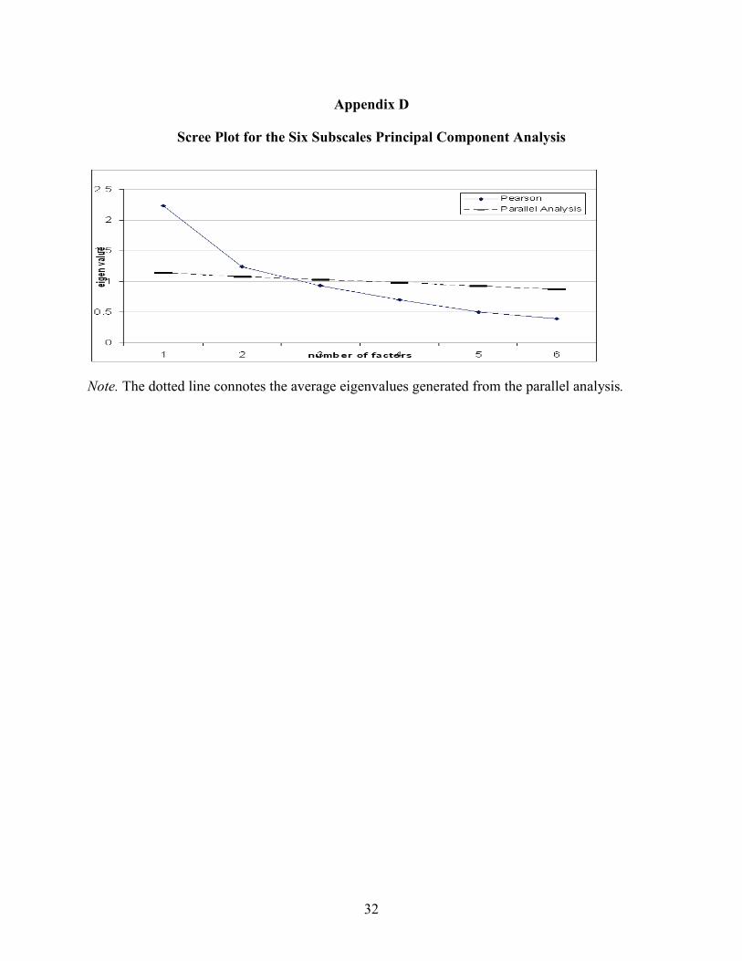
Appendix D

Scree Plot for the Six Subscales Principal Component Analysis

Note. The dotted line connotes the average eigenvalues generated from the parallel analysis.

33

Appendix E

Measurement Models for Each of the Six Subscales

34

Note. T1–T6 represents the six subscales respectively: persistence; estimating-time; calendar;

regrets; impulsivity; clean-desk. The shaded two-way arrows are the modification indices

suggested by the LIEREL program, which might indicate the dependency between the

measurement errors connected.

35

Appendix F

Path Diagram and Parameter Estimates for the Time Management (TM) Scale (Diagonal

Weighted Least Square [DWLS])

Note. Chi-square = 2,802.27, df = 579, p-value = .000, RMSEA (root mean square error

approximate) = .070.

36

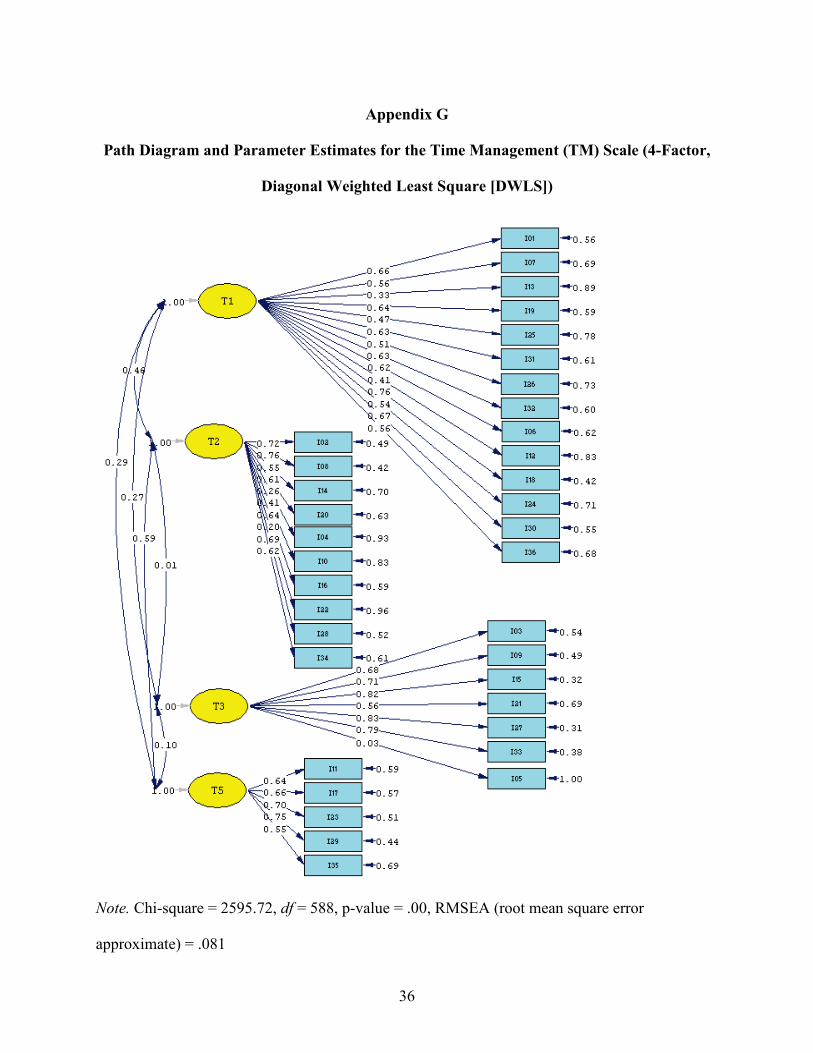
Appendix G

Path Diagram and Parameter Estimates for the Time Management (TM) Scale (4-Factor,

Diagonal Weighted Least Square [DWLS])

Note. Chi-square = 2595.72, df = 588, p-value = .00, RMSEA (root mean square error

approximate) = .081

37

Appendix H

Path Diagram and Parameter Estimates for the Time Management (TM) scale (5-factor,

Diagonal Weighted Least Square [DWL)])

Note. Chi-square = 2335.49; df = 584, p-value = .00, (root mean square error approximate)

RMSEA = .062.