a generic multi-agent reinforcement learning approach … · a generic multi-agent reinforcement...
TRANSCRIPT

Faculty of Science and Bio-Engineering SciencesDepartment of Computer ScienceComputational Modeling Lab
A Generic Multi-Agent ReinforcementLearning Approach for SchedulingProblems
Yailen Martínez Jiménez
Dissertation Submitted for the degree of Doctor of Philosophy in Sciences
Supervisors: Prof. Dr. Ann NowéProf. Dr. Rafael Bello

Print: Silhouet, Maldegem
©2012 Yailen Martínez Jiménez
2012 Uitgeverij VUBPRESS Brussels University PressVUBPRESS is an imprint of ASP nv (Academic and Scientific Publishers nv)Ravensteingalerij 28B-1000 BrusselsTel. +32 (0)2 289 26 50Fax +32 (0)2 289 26 59E-mail: [email protected]
ISBN 978 90 5718 220 4NUR 984Legal deposit D/2012/11.161/156
All rights reserved. No parts of this book may be reproduced or transmitted in any formor by any means, electronic, mechanical, photocopying, recording, or otherwise, withoutthe prior written permission of the author.

To my family and my friendsA mi familia y mis amigos

Committee members:
Supervisors:Prof. Dr. Ann NowéVrije Universiteit Brussel
Prof. Dr. Rafael Bello PérezUniversidad Central “Marta Abreu” de Las Villas
Internal members:Prof. Dr. Viviane JonckersVrije Universiteit Brussel
Prof. Dr. Bernard ManderickVrije Universiteit Brussel
Prof. Dr. Bart JansenVrije Universiteit Brussel
External members:Prof. Dr. Ir. Greet Vanden BergheKAHO Sint-Lieven
Prof. Dr. El-Houssaine AghezzafGhent University

Abstract
Scheduling is a decision making process that is used on a regular basis in manyreal life situations. It takes care of the allocation of resources to tasks over time,and its goal is to optimize one or more objectives. Depending on the problembeing solved, tasks and resources can take many forms, and the objectives can alsovary. In this dissertation we are interested in manufacturing scheduling, which isan optimization process that allocates limited manufacturing resources over timeamong parallel and sequential manufacturing activities. Customer orders have tobe executed, and each order is composed by a number of operations that have tobe processed on the resources or machines available. Each order can have releaseand due dates associated, and typical objectives functions involve minimizing thetardiness or the makespan.
In real world scheduling problems the environment is so dynamic that all thisinformation is usually not known beforehand. For example, manufacturing schedul-ing is subject to constant uncertainty, machines break down, orders take longer thanexpected, and these unexpected events make the original schedule fail. That is thereason why companies prefer to have robust schedules rather than optimal ones. Akey issue is to find a proper balance between these two performance measures.
Scheduling problems can be interpreted as a distributed sequential decision-making task, which makes the use of multi-agent reinforcement learning algorithmspossible. These algorithms are of high relevance to various real-world problems, asthey allow the agents to learn good overall solutions through repeated interactionswith the environment.
Our main contribution is a generic multi-agent reinforcement learning approachthat can easily be adapted to different scheduling settings, such as the job shopscheduling with parallel machines, online problems or the hybrid flow shop schedul-ing. It is possible to increase the robustness of the solutions and to look at differentobjective functions, like the tardiness or the makespan. Furthermore, the proposedapproach allows the user to define certain parameters involved in the solution con-struction process, in order to define the balance between robustness and optimality.
v


Acknowledgements
First of all, I would like to express my sincere gratitude to my supervisors Ann Nowéand Rafael Bello, for accepting me as a PhD student and for all the guidance andthe help during the past years.
I would like to thank the members of the examination committee: Bart Jansen,Viviane Jonckers, Bernard Manderick, El-Houssaine Aghezzaf and Greet VandenBergue, for finding the time to read this dissertation and also for the insightfulcomments and suggestions.
The colleagues and friends from the CoMo lab also deserve a big acknowledge-ment. Thank you, Abdel, Allan, Bert, Cosmin, David C., David S., Joke, Jonatan,Katja, Kevin, Kris, Kristof, Maarten D., Maarten P., Madalina, Marjon, Matteo,Mike, Nyree, Peter, Ruben, Pasquale, Saba, Stijn, Sven, Steven, Tim, Yann-Aël andYann-Michaël, for making CoMo such a nice working environment. Either talkingabout research, playing with the wii, ping pong, or enjoying the BBQs, I hope youwill manage to prepare the mojitos next year ;-) Also thanks to the colleagues fromthe ARTI side: Frederik, Lara, Katrien, Pieter and Luc.
During the PhD I had the opportunity to collaborate with great researchers fromdifferent institutions: Tony, Katja, Greet, Elsy, Dmitriy, Patrick, Stefan, Tommyand all the colleagues from the DiCoMAS project. Thank you for the opportunityof working together and also for spending time together either attending conferencesor summer schools.
Sports were also part of my activities in Brussels, especially badminton and beachvolley (when the weather allowed it). This, together with some other special occa-sions, gave me the opportunity to meet people from other labs and other countries.I would like to thank Elisa, Christophe, Jorge, Engineer, Nicolas, Stefan, Andoni,Lode, Beat, Edgar, Wolf, Theo, Simonne, Anna, Magda, Kasia, Lina, Sebastian,Frank, Anne-Sonia, Kimberly, Eve, Marilyn, Ioana, Virginia and Raül, for makingBrussels a more sporty and friendly environment :)
vii

viii
It was thanks to the support of many people that I was able to get used toBelgium and somehow feel like at home. I want to thank Gabriella, Andrea andthe whole family in Hungary. Borys, Françoise and also many cubans who live inBelgium and who helped me and supported me in many different ways during mystay in Brussels. Muchísimas gracias a Gilberto, Lellani, Abelito, Olga y familia,Francisco y Paola.
I also had the opportunity to meet wonderful people from the Cuban Embassyin Brussels: Maiza, Eduardo, Yurielkys, Michel, Martica, Michel Rodríguez, Arturo,Elvira, Patricia, Niurka, Puig, Yamile, Jorge, Elio y Gilma, Jorge Alfonso, Mirta yOriol, Lourdes, Baby, Elizabeth y Alfredo.
A mis colegas y amigos de la Universidad Central “Marta Abreu” de Las Villas,tanto de la Facultad de Matemática, Física y Computación como de otras facultadesy departamentos. Igualmente a los amigos y vecinos que son casi parte de la familia.Son muchos para mencionarlos a todos, pero dentro de poco tendré la oportunidadde agradecerles en persona!
I am also grateful to the Vrije Universiteit Brussel for providing the funding forthe PhD scholarship and to the VLIR project for the support.
Last but not least, I want to thank my family for their endless support. A todami familia un agradecimiento immenso por siempre creer en mi y por apoyarmeincondicionalmente. Un beso grande a todos.
Thank you all!!Muchas Gracias!!
Brussels, October 2012Yailen

Contents
List of Figures xiii
List of Tables xvii
1 Introduction 11.1 Manufacturing Scheduling . . . . . . . . . . . . . . . . . . . . . . . . 21.2 Operations Research and Artificial Intelligence . . . . . . . . . . . . . 31.3 Our Approach . . . . . . . . . . . . . . . . . . . . . . . . . . . . . . . 51.4 Outline of the Dissertation . . . . . . . . . . . . . . . . . . . . . . . . 6
2 Scheduling Problems 112.1 Introduction to Scheduling . . . . . . . . . . . . . . . . . . . . . . . . 112.2 Notation . . . . . . . . . . . . . . . . . . . . . . . . . . . . . . . . . . 162.3 Classification of Scheduling Problems . . . . . . . . . . . . . . . . . . 17
2.3.1 Machine Environment . . . . . . . . . . . . . . . . . . . . . . 172.3.2 Job Characteristics . . . . . . . . . . . . . . . . . . . . . . . . 182.3.3 Objective Functions . . . . . . . . . . . . . . . . . . . . . . . . 192.3.4 Other Criteria . . . . . . . . . . . . . . . . . . . . . . . . . . . 192.3.5 Types of Schedules . . . . . . . . . . . . . . . . . . . . . . . . 20
2.4 Job Shop Scheduling Problem . . . . . . . . . . . . . . . . . . . . . . 242.4.1 Problem Definition . . . . . . . . . . . . . . . . . . . . . . . . 242.4.2 JSSP Instances . . . . . . . . . . . . . . . . . . . . . . . . . . 26
2.5 Parallel Machines Job Shop Scheduling . . . . . . . . . . . . . . . . . 282.5.1 Problem Description . . . . . . . . . . . . . . . . . . . . . . . 282.5.2 Problem Instances . . . . . . . . . . . . . . . . . . . . . . . . 29
2.6 Flexible Job Shop Scheduling . . . . . . . . . . . . . . . . . . . . . . 302.6.1 Flexible Job Shop Instances . . . . . . . . . . . . . . . . . . . 30
ix

x CONTENTS
2.7 Stochastic Flexible Job Shop Scheduling . . . . . . . . . . . . . . . . 322.8 Online Scheduling . . . . . . . . . . . . . . . . . . . . . . . . . . . . . 332.9 Hybrid Flow Shop Scheduling . . . . . . . . . . . . . . . . . . . . . . 342.10 Solution Methods for Scheduling Problems . . . . . . . . . . . . . . . 37
2.10.1 Dispatching Rules . . . . . . . . . . . . . . . . . . . . . . . . . 372.10.2 Reinforcement Learning approaches . . . . . . . . . . . . . . . 38
2.11 Summary . . . . . . . . . . . . . . . . . . . . . . . . . . . . . . . . . 39
3 Multi-Agent Reinforcement Learning 413.1 Intelligent Agents . . . . . . . . . . . . . . . . . . . . . . . . . . . . . 413.2 Reinforcement Learning . . . . . . . . . . . . . . . . . . . . . . . . . 433.3 Markov Decision Processes . . . . . . . . . . . . . . . . . . . . . . . . 463.4 Solution Methods . . . . . . . . . . . . . . . . . . . . . . . . . . . . . 47
3.4.1 Dynamic Programming . . . . . . . . . . . . . . . . . . . . . . 483.4.2 Q-Learning . . . . . . . . . . . . . . . . . . . . . . . . . . . . 503.4.3 Learning Automata . . . . . . . . . . . . . . . . . . . . . . . . 51
3.5 Action Selection Mechanisms . . . . . . . . . . . . . . . . . . . . . . . 523.6 Multi-Agent Systems . . . . . . . . . . . . . . . . . . . . . . . . . . . 543.7 Reinforcement Learning for Scheduling . . . . . . . . . . . . . . . . . 623.8 Summary . . . . . . . . . . . . . . . . . . . . . . . . . . . . . . . . . 65
4 A Generic MARL Approach for Scheduling Problems 674.1 Applying QL to solve the JSSP . . . . . . . . . . . . . . . . . . . . . 67
4.1.1 Feedback Signals . . . . . . . . . . . . . . . . . . . . . . . . . 704.1.2 Example . . . . . . . . . . . . . . . . . . . . . . . . . . . . . . 714.1.3 Experimental Results QL-JSSP . . . . . . . . . . . . . . . . . 74
4.2 Reinforcement Learning for the JSSP-PM . . . . . . . . . . . . . . . 794.2.1 Experimental Results JSSP-PM . . . . . . . . . . . . . . . . . 80
4.3 Reinforcement Learning for the FJSSP . . . . . . . . . . . . . . . . . 834.3.1 The Proposed Approach: Learning / Optimization . . . . . . 834.3.2 Example . . . . . . . . . . . . . . . . . . . . . . . . . . . . . . 854.3.3 Mode Optimization Procedure . . . . . . . . . . . . . . . . . . 874.3.4 Experimental Results FJSSP . . . . . . . . . . . . . . . . . . . 904.3.5 Comparative Study . . . . . . . . . . . . . . . . . . . . . . . . 91
4.4 Reinforcement Learning for Online Scheduling . . . . . . . . . . . . . 92

CONTENTS xi
4.4.1 Learning Automata for Stochastic Online Scheduling . . . . . 924.4.2 WSEPT Heuristic for Stochastic Online Scheduling . . . . . . 934.4.3 Experimental Results . . . . . . . . . . . . . . . . . . . . . . . 944.4.4 Discussion . . . . . . . . . . . . . . . . . . . . . . . . . . . . . 100
4.5 Summary . . . . . . . . . . . . . . . . . . . . . . . . . . . . . . . . . 100
5 Uncertainty and Robustness in Scheduling 1035.1 Uncertainty in Scheduling . . . . . . . . . . . . . . . . . . . . . . . . 1045.2 Robustness . . . . . . . . . . . . . . . . . . . . . . . . . . . . . . . . 106
5.2.1 Measuring Robustness . . . . . . . . . . . . . . . . . . . . . . 1065.3 Proactive vs. Reactive Approaches . . . . . . . . . . . . . . . . . . . 107
5.3.1 Reactive Approaches . . . . . . . . . . . . . . . . . . . . . . . 1095.3.2 Proactive Approaches . . . . . . . . . . . . . . . . . . . . . . . 110
5.4 Slack Based Techniques . . . . . . . . . . . . . . . . . . . . . . . . . . 1115.4.1 Temporal Protection . . . . . . . . . . . . . . . . . . . . . . . 1115.4.2 Time Window Slack . . . . . . . . . . . . . . . . . . . . . . . 1135.4.3 Focused Time Window Slack . . . . . . . . . . . . . . . . . . . 1155.4.4 Discussion about the slack-based techniques . . . . . . . . . . 116
5.5 Summary . . . . . . . . . . . . . . . . . . . . . . . . . . . . . . . . . 116
6 Scheduling under Uncertainty 1176.1 Deterministic Case with Known Disruptions . . . . . . . . . . . . . . 1186.2 Stochastic Flexible Job Shop Scheduling . . . . . . . . . . . . . . . . 119
6.2.1 Stochastic Flexible Job Shop Instances . . . . . . . . . . . . . 1196.2.2 Online Forward Optimization . . . . . . . . . . . . . . . . . . 1206.2.3 SaFlexS . . . . . . . . . . . . . . . . . . . . . . . . . . . . . . 1216.2.4 Learning / Optimization . . . . . . . . . . . . . . . . . . . . . 1226.2.5 Experimental Results . . . . . . . . . . . . . . . . . . . . . . . 122
6.3 The Proposed Slack-based Approach . . . . . . . . . . . . . . . . . . 1256.3.1 ‘Criticality’ . . . . . . . . . . . . . . . . . . . . . . . . . . . . 125
6.4 The Proposed Approach . . . . . . . . . . . . . . . . . . . . . . . . . 1276.4.1 Measuring Robustness . . . . . . . . . . . . . . . . . . . . . . 134
6.5 Hybrid Flow Shop Scheduling . . . . . . . . . . . . . . . . . . . . . . 1386.5.1 Experimental Results . . . . . . . . . . . . . . . . . . . . . . . 1406.5.2 Conclusions about the Hybrid Flow Shop Experiments . . . . 143

xii CONTENTS
6.6 Summary . . . . . . . . . . . . . . . . . . . . . . . . . . . . . . . . . 143
7 Conclusions 1457.1 Contributions . . . . . . . . . . . . . . . . . . . . . . . . . . . . . . . 1467.2 Future Work . . . . . . . . . . . . . . . . . . . . . . . . . . . . . . . . 148
Curriculum Vitae 151
Bibliography 155
Index 167

List of Figures
1.1 Integration of Artificial Intelligence and Operations Research tech-niques. . . . . . . . . . . . . . . . . . . . . . . . . . . . . . . . . . . . 4
1.2 Graphical representation of the outline of this dissertation. . . . . . . 9
2.1 Information flow diagram in a manufacturing system. . . . . . . . . . 132.2 Several factors that can influence a scheduling problem. . . . . . . . . 142.3 Different types of Scheduling Problems . . . . . . . . . . . . . . . . . 152.4 Timing diagram of one operation. . . . . . . . . . . . . . . . . . . . . 172.5 Three different feasible solutions to the instance presented in Table 2.1. 212.6 Different types of schedules. The optimal solutions can be found
within the active schedules, but not necessarily in the non-delay class. 222.7 Left: Optimal schedule. Right: Non-delay schedule . . . . . . . . . . 232.8 Example of a JSSP instance (ft06) from the OR-Library. . . . . . . . 262.9 Job description in the JSSP environment. . . . . . . . . . . . . . . . . 272.10 Optimal schedule for the instance ft06. Each color represents a dif-
ferent job. . . . . . . . . . . . . . . . . . . . . . . . . . . . . . . . . . 272.11 Example of a JSSP-PM instance with k=2. . . . . . . . . . . . . . . . 292.12 Flexible Job Shop Scheduling Instance . . . . . . . . . . . . . . . . . 312.13 Job description in the Flexible Job Shop environment . . . . . . . . . 312.14 A two-stage chemical production plant. For both product types P1
and P2, there are two parallel machines at the first stage. At thesecond stage of the process, there are also two parallel machines. . . . 33
2.15 Hybrid Flow Shop Scheduling environment . . . . . . . . . . . . . . . 352.16 Production process stages . . . . . . . . . . . . . . . . . . . . . . . . 36
3.1 The standard reinforcement learning model. . . . . . . . . . . . . . . 443.2 Robot navigation example. . . . . . . . . . . . . . . . . . . . . . . . . 46
xiii

xiv LIST OF FIGURES
3.3 Learning Automaton in its environment. . . . . . . . . . . . . . . . . 523.4 Multiple agents acting in the same environment. . . . . . . . . . . . . 563.5 Relationship between the different MDP models. . . . . . . . . . . . . 583.6 Two agents with their corresponding set of actions, which constitute
their current state. . . . . . . . . . . . . . . . . . . . . . . . . . . . . 613.7 Agents in a scheduling environment. . . . . . . . . . . . . . . . . . . . 623.8 Different approaches relating to the problem space . . . . . . . . . . . 63
4.1 JSSP Instance ft06, composed by 6 jobs and 6 machines. . . . . . . . 684.2 Agents choosing from their corresponding sets of currently selectable
operations. . . . . . . . . . . . . . . . . . . . . . . . . . . . . . . . . . 724.3 Updating the states of the agents after one action selection step. . . . 724.4 Left: Optimal schedule. Right: Non-delay schedule . . . . . . . . . . 734.5 Agents acting in an environment where only non-delay schedules are
obtained. . . . . . . . . . . . . . . . . . . . . . . . . . . . . . . . . . . 734.6 Agents acting in an environment where delay schedules can be obtained. 744.7 Learning - Instance ft06 - optimal solution Cmax = 55 . . . . . . . . . 764.8 Learning process instance la01 - optimal solution Cmax = 666 . . . . . 764.9 Queue per agent, and one agent per resource . . . . . . . . . . . . . . 804.10 Queue per type of resource, agent per resource. . . . . . . . . . . . . 814.11 Schedule for the operation - machine assignments using the fastest
machine. . . . . . . . . . . . . . . . . . . . . . . . . . . . . . . . . . . 874.12 Optimal schedule for the example. . . . . . . . . . . . . . . . . . . . . 874.13 Feasible schedule obtained by the learning step. . . . . . . . . . . . . 884.14 Backward schedule. . . . . . . . . . . . . . . . . . . . . . . . . . . . . 894.15 Forward schedule. . . . . . . . . . . . . . . . . . . . . . . . . . . . . . 904.16 A two-stage chemical production plant. For both product types P1
and P2, there are two parallel machines at the first stage. At thesecond stage of the process, there are also two parallel machines. . . . 92
4.17 Queues of the machines when following the random strategy. . . . . . 954.18 Queues of the machines when using Linear Reward-Inaction. . . . . . 964.19 Queues of the machines when using LR−εP . . . . . . . . . . . . . . . . 964.20 Queued jobs at the end of the process. . . . . . . . . . . . . . . . . . 974.21 Total number of jobs executed at the end of the 25000 iterations. . . 97
5.1 Scheduling Environment . . . . . . . . . . . . . . . . . . . . . . . . . 104

LIST OF FIGURES xv
5.2 Predictive vs. Reactive Scheduling . . . . . . . . . . . . . . . . . . . 1085.3 Increasing robustness by adding redundancy. Schedule b) is consid-
ered more robust than schedule a). . . . . . . . . . . . . . . . . . . . 1105.4 Example of two consecutive operations which are executed on a break-
able resource. The white part of each box represents the original pro-cessing time of the operation and the gray part represents the extratime added by the temporal protection technique. . . . . . . . . . . . 112
5.5 Example of schedule where a breakable resource has three operationsscheduled. . . . . . . . . . . . . . . . . . . . . . . . . . . . . . . . . . 113
5.6 Example where the slack time added by the temporal protectionmethod can not be used by the next activity on the same machinedue to ordering constraints. . . . . . . . . . . . . . . . . . . . . . . . 114
5.7 Adding slack time under the Time Windows Slack method. . . . . . . 1145.8 Adding slack time using the Focused Time Windows Slack approach. 115
6.1 Adding scheduled maintenances to the instances. . . . . . . . . . . . . 1196.2 Stochastic Flexible Job Shop instance. . . . . . . . . . . . . . . . . . 1216.3 Instances Mk01 and Mk10 - No Perturbations . . . . . . . . . . . . . 1236.4 Instances Mk04 and Mk06 - With Perturbations . . . . . . . . . . . . 1246.5 Instances Mk01 and Mk04 - With Perturbations and using tardiness
as objective function. . . . . . . . . . . . . . . . . . . . . . . . . . . . 1256.6 Optimal solution for the instance ft06, Cmax = 55 . . . . . . . . . . . 1266.7 Optimal schedule affected by several perturbations, Cmax = 64. . . . . 1296.8 Schedule created using the temporal-protection technique. . . . . . . 1306.9 Schedule obtained by adding slack times on the critical machines after
the scheduling process. . . . . . . . . . . . . . . . . . . . . . . . . . . 1326.10 Schedule obtained by adding slack times on the critical machines dur-
ing the scheduling process . . . . . . . . . . . . . . . . . . . . . . . . 1336.11 Comparing the execution of non-protected schedules and solutions
constructed using our approach based on criticality, in terms of thedeviation from the original schedules. . . . . . . . . . . . . . . . . . . 134
6.12 Measuring the deviation from the original schedules. . . . . . . . . . . 1366.13 Comparison between the approaches according to their deviation from
their own original schedule using six levels of perturbations. . . . . . 137

xvi LIST OF FIGURES
6.14 Comparison of the different approaches in terms of both makespanand deviation from their originally proposed schedule. . . . . . . . . . 138
6.15 Example of a possible solution for the hybrid flow shop problem. . . . 141
7.1 Graphical representation of the contributions of this dissertation. . . 148

List of Tables
2.1 Scheduling instance with 2 resources and 2 jobs. . . . . . . . . . . . . 212.2 Instance with 3 resources and 2 jobs. Job 1 consists of 3 operations,
operation 1 (Op1) has to be executed on machine M1 during 1 timestep, Op2 on machine M2 for 3 times steps and so on. . . . . . . . . . 23
3.1 Interaction between one agent and its environment . . . . . . . . . . 453.2 Comparison between different representations of agents systems. . . . 60
4.1 Instance with 3 resources and 2 jobs. . . . . . . . . . . . . . . . . . . 734.2 Job Shop Scheduling instances and their optimal solutions, in terms
of makespan. . . . . . . . . . . . . . . . . . . . . . . . . . . . . . . . 754.3 Comparison between the different variants of the algorithm. . . . . . 774.4 Comparative study for the JSSP. . . . . . . . . . . . . . . . . . . . . 784.5 MRE per group of instances . . . . . . . . . . . . . . . . . . . . . . . 794.6 Comparison of both points of view for duplicated instances . . . . . . 824.7 Comparison of both points of view for triplicated instances. . . . . . . 824.8 Comparative study for the JSSP-PM. . . . . . . . . . . . . . . . . . . 844.9 Experimental Results FJSSP. . . . . . . . . . . . . . . . . . . . . . . 914.10 MRE: Mean relative errors . . . . . . . . . . . . . . . . . . . . . . . . 924.11 Processing speeds of all machines for two different settings. . . . . . . 954.12 Average probabilities of all agents through an entire simulation. . . . 99
6.1 Set of perturbations . . . . . . . . . . . . . . . . . . . . . . . . . . . . 1276.2 Processing times of the six types of products in the different phases
of the process. . . . . . . . . . . . . . . . . . . . . . . . . . . . . . . . 1396.3 Overall comparison table in terms of tardiness. . . . . . . . . . . . . . 142
xvii


Chapter 1
Introduction
A schedule is commonly defined as ‘a plan for performing work or achieving anobjective, specifying the order and allotted time for each part’. With this definitionin mind, if we think about scheduling, which is the action of making a schedule,it is easy to notice that it is a type of task that we have all performed at somepoint, maybe without noticing it. Let us start with a simple example: how manytimes have you decided beforehand the tasks you want to do in one day? and eventhe order in which you want to accomplish them? Yes, that is scheduling. And ofcourse, you prepare your schedule with one objective in mind, maybe you have tofinish a report by 4pm, which means that you have a deadline to meet, or maybeyou just want to go home early, meaning that you want to finish with everything assoon as possible.
But even this simple scenario can get a bit more complicated. For example, whensome types of tasks start to repeat, because there are specific things you have toperform every day, then you start to evaluate how good the schedule you made theprevious day was (again, maybe without noticing it). You might change the orderin which you perform the tasks, because you think there is a slight chance of finish-ing earlier if you make some changes in your daily actions, which means that youadjust your decisions depending on the outcome you were able to obtain, then wecan say that you are learning from experience. Now imagine a system composed byseveral persons like you, performing tasks in specific orders, but now you have to usecommon resources to accomplish the tasks. As you can notice, a good coordinationis needed in order to make sure that all the tasks are executed and the objective ofthe whole system is optimized.
1

2 Chapter 1. Introduction
Scheduling is a decision making process that is used on a regular basis in ev-ery situation where a specific set of tasks has to be performed on a specific set ofresources. Some examples are: airport gate scheduling, crew scheduling, processorscheduling and manufacturing scheduling. In this dissertation we will focus on man-ufacturing scheduling, where the schedule construction process plays an importantrole, as it can have a major impact on the productivity of the company. In thecurrent competitive environment, effective scheduling has become a necessity forsurvival in the market place, as companies have to meet the due dates and use theresources in an efficient manner [Pinedo (2008)].
1.1 Manufacturing SchedulingManufacturing scheduling is defined as an optimization process that allocates lim-ited manufacturing resources over time among parallel and sequential manufacturingactivities. This allocation must obey a set of constraints that reflect the temporalrelationships between activities and the capacity limitations of a set of shared re-sources [Wang & Shen (2007)].
In other words, the problem can be defined as a set of jobs that has to beprocessed on a set of machines, with the objective of finding the best schedule, thatis, an allocation of the jobs to time intervals on the machines that minimizes thechosen objective. Each job consists of a set of operations that have to be scheduledin a predetermined order, and each of these operations needs a certain amount oftime (processing time) to be executed. This time depends on the machine wherethe operation will be processed. The jobs can have release and due dates associated,which means that they are expected to be finished in a specific amount of time.
If we are solving a deterministic scheduling problem, then all the informationis assumed to be known beforehand: the number of jobs, the number of machines,the number of operations per job, the processing times of the operations, the prece-dence constraints and problem constraints (which can change depending on the typeof scheduling problem being solved). If, on the other hand, the scheduling problembeing solved is stochastic, then the information is not complete, because the process-ing times of the operations belonging to the different jobs are modeled as randomvariables. This means that the processing time of an entire job is not known untilit is fully executed.

Chapter 1. Introduction 3
The problems can be classified according to different characteristics, for example,the number of machines (one machine, parallel machines), the job characteristics(preemption allowed or not, equal processing times) and so on. In this dissertationwe will assume the classification scheme proposed in [Graham et al. (1979)], wherethe scheduling problems are specified using a classification in terms of three fieldsα|β|γ, where α specifies the machine environment, β the operation characteristics,and γ the criteria to optimize.
The combination of all these features makes the scheduling problem a challeng-ing task, that is why it has captured the interest of many researchers from differentresearch communities, for example, Operations Research (OR) and Artificial Intel-ligence (AI).
1.2 Operations Research and Artificial IntelligenceManufacturing scheduling problems have been addressed using combinatorial op-timization techniques, both approximate methods and exact methods. Accordingto [Billaut et al. (2008)], solving a particular problem may require the use of mod-eling tools for complex systems (simulation, Petri nets, etc.), thus leading to thedefinition of matchings between these methods.
Different OR techniques (Linear Programming, Mixed-Integer Programming,etc) have been applied to scheduling problems. These approaches usually involvethe definition of a model, which contains an objective function, a set of variables anda set of constraints. OR based techniques have demonstrated the ability to obtainoptimal solutions for well-defined problems, but OR solutions are restricted to staticmodels. AI approaches, on the other hand, provide more flexible representations ofreal-world problems, allowing human expertise to be present in the loop [Gomes(2000)].
The vast majority of the research in scheduling has focused on the development ofexact and suboptimal procedures for the generation of a baseline schedule assumingcomplete information and a deterministic environment [Herroelen & Leus (2005)].However, the real world is not so stable, projects may be subject to unexpectedevents during execution, which may lead to numerous schedule disruptions, for ex-ample, resources can become unavailable (breakdowns or scheduled maintenances),new orders can arrive, operations could take longer than expected, etc.

4 Chapter 1. Introduction
One approach to deal with such disruptions is to generate robust schedules,where robustness refers to the performance of an algorithm under uncertainties[Davenport et al. (2001)]. The objective is to generate schedules that are ableto absorb some level of uncertainty without having to reschedule. There are sometechniques that can deal with such problems, in this dissertation we will considerslack-based techniques, where the main idea is to provide each activity with someextra execution time (slack time) in such a way that part of the uncertainty can beabsorbed. The slack time that will be added to each activity or task is proportionalto its duration and the resource where it will be processed.
A very important issue is to focus the slack time on areas where it will be reallyneeded. For example, let us assume that a new machine arrives in the system, whichcan work for long periods before breaking, then it is not wise to make the schedulemore robust at the beginning of the scheduling period. The key point is then toidentify these areas that are more likely to need slack time in order to deal with amachine breakdown or other unexpected events.
In order to summarize all the features that have been described, Figure 1.1 showsa perspective of integration between AI and OR techniques.
Figure 1.1: Integration of Artificial Intelligence and Operations Researchtechniques, taken from [Gomes (2000)].
This idea was presented in [Gomes (2000)], where the author explains how ORmethods have focused on tractable representations, which have demonstrated theability to identify optimal and locally optimal solutions, but they are restricted to

Chapter 1. Introduction 5
rigid models with limited expressive power. AI methods, on the other hand, providericher and more flexible representations, which can lead to intractable problems.The challenge is to achieve some sort of unification between the approaches in orderto come up with good representations of the problem and at the same time dealwith uncertainty, scalability issues and increase the robustness.
1.3 Our ApproachMany scheduling problems suggest a natural formulation as distributed decision-making tasks. Hence, the employment of multi-agent systems represents an evidentapproach. Furthermore, given the well-known inherent intricacy of solving schedul-ing problems, decentralized approaches for solving them may yield a promising op-tion [Gabel (2009)]. The research presented in this dissertation is based on this idea.We propose a generic multi-agent reinforcement learning approach for schedulingproblems, which attempts to solve some of the issues mentioned in the previous sec-tion by focusing on finding robust solutions to different scheduling problems usinga combination of different techniques, mainly reinforcement learning, optimization,and slack-based approaches.
Reinforcement Learning (RL) is learning what to do (how to map situationsto actions) so as to maximize a numerical reward signal [Sutton & Barto (1998)].It allows an agent to learn optimal behavior through trial-and-error interactionswith its environment. By repeatedly trying actions in different situations the agentcan discover the consequences of its actions and identify the best action for eachsituation. For example, when dealing with unexpected events, learning methodscan play an important role, as they could ‘learn’ from previous results and changespecific parameters for the next iterations, allowing not only to find good solutions,but more robust ones.
A common approach to solve scheduling problems is to use dispatching priorityrules, which work by assigning priorities to the tasks that can be executed on aresource depending on a specific criteria. The learning algorithms could benefitfrom this idea, by associating the priorities with the feedback signal the agentsreceive when executing the actions, and this is something that will be studied inthis dissertation.

6 Chapter 1. Introduction
Another problem that has been identified in the scheduling community is thefact that most of the research concentrates on optimization problems that are asimplified version of reality. As the author points out in [Urlings (2010)]: “this allowsfor the use of sophisticated approaches and guarantees in many cases that optimalsolutions are obtained. However, the exclusion of real-world restrictions harms theapplicability of those methods. What the industry needs are systems for optimizedproduction scheduling that adjust exactly to the conditions in the production plantand that generate good solutions in very little time”.
It is well known that companies prefer to have robust schedules, even thoughrobustness implies extra time in the schedule. The inclusion of extra time meansthat you lose in optimality, but the real world is so dynamic that you have to expectthe unexpected.
In this thesis we help to close the gap between literature and practice. Thegeneric multi-agent reinforcement learning approach being proposed allows to sim-ulate, for example, what will happen if a resource is not available during a specificamount of time, or to estimate the probable end time of an extra order that arrivesto the system after some hours of work, having a very high priority. This helps toidentify the ‘critical’ parts of the schedule and based on that incorporate differentlevels of robustness to the solution in those places where it will be needed.
In the next section we give an overview of the structure of this dissertation.
1.4 Outline of the DissertationThe research presented in this dissertation is divided in seven chapters.
In Chapter 2 we present an overview of the different scheduling problems thatwill be addressed in this dissertation. We start explaining the Job Shop SchedulingProblem, then we gradually move towards more challenging problems, like the Par-allel Machines Job Shop Scheduling, where identical parallel machines can executethe same type of tasks, and the Flexible Job Shop Scheduling Problem, where thereare also multiple machines that can execute the same type of tasks, but in this casethe machines are not identical, for example, they can differ in speed, and this givesan extra level of complexity to the sequencing process.
Then we switch to more stochastic scenarios. We introduce a version of theFlexible Job Shop Scheduling Problem where release dates and due dates are added

Chapter 1. Introduction 7
to the jobs. Some perturbations are also introduced in the system, mainly repre-sented by machine breakdowns, which gives the possibility of looking at differentobjective functions, as there is more information involved. We also present an onlinescheduling problem, which is based on a chemical production plant with two decisionlevels. Each level has four machines which differ in speed and jobs enter the systemaccording to specific stochastic distributions.
Finally, we describe a scheduling scenario that is based on a real-world case,which according to its specifications belong to the category of the hybrid flow-shopscheduling problems (jobs have to be processed following the same production flowin a series of stages). It is an enzyme production process with four different stages:1) seed fermentation, 2) main fermentation, 3) broth preparation and 4) recovery.Each of these stages has multiple machines, except the recovery line. The ordersfrom the customers can involve the production of different types of enzymes, and allof them have to follow the production path in the same order (stages 1 to 4). Toconclude the chapter, some related work is presented.
Chapter 3 provides the main ideas behind Reinforcement Learning and the the-ory on Multi-Agent Reinforcement Learning. The concepts of agent and multi-agentsystems are introduced, as well as different representations of agents systems. Weexplain how the agents interact with the environment in order to learn how to solvea specific task, and how multiple agents can act in a cooperative or competitive way.Different solution methods are introduced, together with three possible action selec-tion strategies. The last section of the chapter defines the main concepts that haveto be taken into account when solving a scheduling problem using a Multi-AgentReinforcement Learning Approach.
In Chapter 4 we summarize the main results of the application of ReinforcementLearning in the solution of the different scheduling problems introduced in Chapter2. We start by introducing a basic approach, which is modeled for the JSSP, andthen we explain how to adapt this model in order to deal with the extra constraintsthat gradually appear in the other scheduling scenarios. Each section of the chapterpresents the approach corresponding to one of the scheduling problems and someof the results obtained by experimenting and comparing with other approaches re-ported in literature.
8 Chapter 1. Introduction
As discussed before, there are several unexpected events that can affect thescheduling process. In the real-world things are constantly changing and this issomething inevitable, machines can break down, customers can show up with neworders, jobs can take longer than expected, and these events can occur at any time,making the original schedule fail. In Chapter 5 we give some details about the dif-ferent sources of uncertainty that can affect the scheduling process. We introducethe concept of robustness and how to incorporate it in the solutions. We presentsome existing techniques in this area and discuss how each of them introduces theslack time (extra time assigned to the activities) that can be used for the algorithmto deal with unexpected events.
As was mentioned before, it is important to take unexpected events into account.This is the sole focus of the research presented in Chapter 6: how to schedule un-der uncertainty. This chapter is divided in two parts. First, we present the resultsobtained when solving a stochastic scheduling problem. This study was developedin collaboration with Elsy Kaddoum, from the Systèmes Multi-Agents Coopératifs(SMAC) lab - IRIT, Université Paul Sabatier, Toulouse, France, and Tony Wauters,from the Combinatorial Optimisation and Decision Support (CODeS) ResearchGroup, KAHO Sint-Lieven, Gent. The results of this collaboration were presentedin [Kaddoum et al. (2010)]. In the second part of the chapter, a new slack-based ap-proach which aims at incorporating robustness in the solution construction processis introduced. Our idea is based on the methods introduced in the previous chapter,but it changes the way the slack time is added. The term ‘criticality’ is introducedand its influence in the way of providing the activities with extra time is explained.It is important to mention that this approach allows the user to define the level ofrobustness that will be included in the solution. Of course this is more useful whenthe user has domain knowledge, and it could be achieved by letting him tune the pa-rameters that define when a specific part of the schedule can be considered as critical.
Finally, we conclude in Chapter 7 with a summary of the presented research, to-gether with some ideas for future work, including a potential real-world applicationin the Cuban industry.
Figure 1.2 provides a graphical representation of this outline. The arrows repre-sent the dependency between the different chapters.

Chapter 1. Introduction 9
Figure 1.2: Graphical representation of the outline of this dissertation.


Chapter 2
Scheduling Problems
Scheduling concerns the allocation of limited resources to tasks over time.It is a decision-making process that has as a goal the optimization of one
or more objectives- [Pinedo (2008)] -
Scheduling problems are present in every situation where a given set of tasks hasto be performed and these tasks require the allocation of resources to time slots.This is a common procedure that we usually perform in our daily life, but whenthe constraints that have to be met increase and the number of tasks and resourcesgrow, then we realize that constructing a schedule that satisfies all the requirementsis not so straightforward. This chapter starts by giving an introduction to schedulingand some of the factors that can influence this kind of problem. The different typesof schedules that can be obtained are defined, as well as the different schedulingproblems that will be addressed by the research presented in this dissertation.
2.1 Introduction to Scheduling
Scheduling is a decision making process that is used on a regular basis in manyreal life situations. It deals with the allocation of resources to tasks over time,and its goal is to optimize one or more objectives [Pinedo (2008)]. For example,
11

12 Chapter 2. Scheduling Problems
scheduling problems occur routinely in publishing houses, universities, hospitals,airports, transportation companies, manufacturing and services industries, and soon. The resources and tasks can take many forms, depending on the problem beingsolved, and the objectives can also vary, for example, one of the most common goalsis to minimize the makespan, which is the completion time of the last task.
The problem of scheduling has captured the interest of many researchers froma number of research communities: management science, industrial engineering,operations research (OR) and artificial intelligence (AI). The growing complexity ofmanufacturing processes and fierce competition in the market place drive enterprisesto optimize their operations as much as possible. In particular, optimal schedulingof production orders on limited resources is an important issue and this type ofoptimization problem has fascinated researchers for years [Grossmann (2005)].
Manufacturing scheduling, in short, is an optimization process that allocates lim-ited manufacturing resources over time among parallel and sequential manufacturingactivities. This allocation must obey a set of constraints that reflect the temporalrelationships between activities and the capacity limitations of a set of shared re-sources. The allocation also affects the optimality of a schedule with respect todifferent criteria.
Figure 2.1 shows a typical diagram of the information flow in a manufactur-ing/production system.
In general, in a manufacturing system, the scheduling function has to interactwith other decision making functions. It is affected by the middle-range planning,which examines the stock levels, the demand forecasting and the requirements plan,in order to achieve the optimization of the combination ‘Production-Allocation ofResources’. In this context, the construction of a feasible, optimized productionschedule, without the support of an advanced decision support tool, is a very difficultand time consuming procedure that requires not only deep knowledge of all thedata and parameters of the production system, but also specific knowledge in theparticular field [Metaxiotis et al. (2005)].
These type of problems are typically NP-hard [Garey et al. (1976), Brucker(2007)] and the computational time increases exponentially with the problem size,being manufacturing scheduling one of the most difficult scheduling problems [Shen(2002)].

Chapter 2. Scheduling Problems 13
Figure 2.1: Information flow diagram in a manufacturing system, takenfrom [Pinedo (2008)].
Research in this field has made an impressive progress, from simple models thatare only useful from an academic point of view to approaches that can be used incomplex realistic settings like batch production, where groups of items (batches)move through the production process together, a stage at a time, and the next stagecan not start until the previous one is completed1. Batch processes are widely usedin the pharmaceutical, chemical, food, paint, and agrichemical industries, becausethey provide the flexibility to produce various products using the same processingfacility [Charnprasitphon (2007)].
Figure 2.2 shows several factors that can influence a scheduling problem, of coursethese factors do not necessarily appear at the same time.
Every real-life production process has its own specific characteristics and con-straints which are hard to generalize into a one-size-fits-all mathematical problem
1 the order of the stages is fixed

14 Chapter 2. Scheduling Problems
Figure 2.2: Several factors that can influence a scheduling problem.
formulation, so effective optimization approaches remain in high demand.The classical approach to solve scheduling problems consists of setting up a math-
ematical model, often based on a Mixed Integer Linear Programming formulation,and then applying a search algorithm like Branch and Bound to calculate the (guar-anteed) optimal solution [Méndez et al. (2006)]. However, as the problem grows inthe number of available resources, operations to be scheduled, and other constraintsto be taken into account, this approach will no longer yield an optimal solution ina reasonable time span. In this situation, researchers often relax constraints thatactually exist in the real-life problem. This makes the problem solvable, but it is nolonger of practical use. As a consequence, only a fraction of published schedulingresearch deals with actual real-world problems [Ruiz et al. (2008)].
Figure 2.3 summarizes the different types of scheduling problems that will beaddressed in this dissertation. The left side of the picture shows the deterministicproblems and the right side groups the stochastic ones and a real-world case. It isworth to mention that the online scheduling problem addressed in this dissertationis based on a real scenario, although it is a simplified version of the original problem.

Chapter 2. Scheduling Problems 15
Figure 2.3: Different types of Scheduling Problems
All these scheduling problems will be explained in detail in the next sections ofthe chapter (from section 2.4 to 2.9). But first we introduce some basic notationand properties (sections 2.2 and 2.3) that will be used in the rest of the dissertation.

16 Chapter 2. Scheduling Problems
2.2 NotationThe definition of a scheduling problem includes several variables and properties, inthis section we provide a list of the ones that will be used in this dissertation:
m Number of machines
n Number of jobs
Mi Machine i, where i = 1, ...,m
Jj Job j, where j = i, ..., n
Cj The completion time of job j
Pj Processing time of job j
oij The ith operation of job j
sij Start time of the operation i, job j
cij Completion time of the operation i, job j
pij Processing time of operation i, job j
rj Release date of job j
dj The due date of job j
Cmax The makespan, maximum Cj over all jobs, max(C1, ..., Cn)
Lj Lateness of job j
Ej Earliness of job j
Tj Tardiness of job j
wj The weight associated with job j
Figure 2.4 shows an example of a timing diagram for operation oij, where someof the properties mentioned before are summarized. The rest of the properties willbe described in the next section.

Chapter 2. Scheduling Problems 17
Figure 2.4: Timing diagram of one operation.
2.3 Classification of Scheduling Problems
Scheduling problems are commonly classified according to the machine environment,the job characteristics and the objective function [Herrmann et al. (1993)]. Thisclassification is commonly referred to as the triplet α|β|γ, proposed in [Graham et al.(1979)], where:
• α describes the machine environment (single machine, multiple machines), seesubection 2.3.1.
• β denotes the constraints that have to be met (subsection 2.3.2).
• γ refers to the objective function, for example, the makespan, which is the morecommonly used in literature, for more explanation about possible objectivesfunctions see subsection 2.3.3.
2.3.1 Machine Environment
The first element of the problem description is the machine environment. The caseof a single machine is the simplest of all possible machine environments, as jobshave only one operation to be performed and there is only one machine that canexecute it. But when there are multiple machines that can process the operations,the environments get more complicated, as parallel machines could be identical,but they could also differ in speed. The possible environments are summarized asfollows:

18 Chapter 2. Scheduling Problems
• Identical Parallel Machines: process jobs with the same speed.
• Non-Identical Machines: have machine-dependent speeds.
• Unrelated Parallel Machines: have machine and job dependent speeds.
When each job has a fixed number of operations requiring different machines weare dealing with a shop problem, and depending on the constraints it presents, canbe included in one of the following categories:
• Open Shop: There are m machines and each job has to be processed on eachof them. There are no ordering constraints between the operations of each job,which means that jobs can follow different routes.
• Job Shop: In a job shop with m machines, jobs have to visit each machineonce, but in this case the operations of a job are totally ordered. This orderis not the same for all the jobs.
• Flow Shop: In a Flow Shop with m machines, all jobs go through all themachines in the same order.
• Flexible Job Shop: A generalization of the job shop and the unrelated parallelmachines environment. Each operation can be processed by any among a setof possible machines, and these machines differ in speed.
2.3.2 Job Characteristics
Each problem has a set of job characteristics, which may occur in any combination.A list of the more commonly used is given below:
• Preemption: refers to environments where the processing of a job may beinterrupted and resumed later (possibly on another machine).
• Precedence Constraints: The jobs can have precedence constraints, that is,some jobs can not start until others are completed.
• Release Dates: A job can not start to be processed before its release date.
• Due Dates: Time by which a job is expected to be finished.
• Setup Times: There might be a setup time involved between the execution oftwo different jobs on the same machine, which means that the machine needssome time to get ready for the execution of the next job.
Chapter 2. Scheduling Problems 19
2.3.3 Objective Functions
The objective function to be minimized or maximized is the third element of aproblem description. This may be a sum of variables or the maximum or mini-mum of some variable function. Typical objective functions include the followingperformance measures:
• Flowtime: sum of the completion times of the jobs, ∑j Cj.
• Makespan: maximum completion time, which is equivalent to the time whenthe last job leaves the system (also known as Cmax).
• Lateness: difference between the due date and the completion time. Thismeasure can be positive (tardiness) or negative (earliness), Lj = Cj − dj.Tardiness measures the difference if the job is late, otherwise it takes valuezero. Similarly, earliness measures the difference if the job is finished early,otherwise it is zero.
– Earliness: ∑nj=1 Ej, where Ej = max(dj − Cj, 0)
– Tardiness: ∑nj=1 Tj, where Tj = max(Cj − dj, 0) = max(Lj, 0)
• Earliness-Tardiness: This measure has been the focus of some studies whereit is desirable that jobs finish close to their due dates, ∑n
j=1 Ej + ∑nj=1 Tj,
penalties could also be associated when jobs are either too early or too late.
• Total weighted tardiness: Similar to the tardiness but this time the weight ofthe jobs is taken into account: ∑j wjTj.
2.3.4 Other Criteria
Another distinction to be made is between deterministic and stochastic schedulingproblems. In the deterministic class, all parameters are known without uncertainty,whereas this is not the case in the latter. Stochastic scheduling is concerned withscheduling problems in which the processing times of tasks are modeled as randomvariables.
Finally, scheduling methodologies can also be classified according to the waythe schedule is obtained. The methods can obtain the solutions in a constructiveway or by iteratively repairing a complete schedule. The constructive methodsincrementally extend a partial schedule until every task has been scheduled. The

20 Chapter 2. Scheduling Problems
repair methods iteratively modify a complete schedule to remove conflicts or tofurther optimize the solution. Most optimization methods and constraint-directedsearch methods follow the constructive approach.
2.3.5 Types of Schedules
According to the schedule properties, any feasible schedule (i.e. a solution to thescheduling problem) can be categorized into three major kinds: non-delay, semi-active and active. The definitions of these categories are adapted from [Conway et al.(1967)] and [Pinedo (2008)]. We first present the three definitions and afterwardssummarize the main differences between them with one general example.
Definition 1 (Non-Delay Schedule). A feasible schedule is called non-delay, if noresource is kept idle, while there is at least one operation waiting for further pro-cessing on that resource.
The non-delay category is probably one of the most used in literature whensolving a scheduling problem where the objective is to minimize the makespan.However, at the end of the section we will show that keeping the resources workingdoes not always lead to optimal solutions.
Definition 2 (Semi-Active Schedule). A feasible schedule is called semi-active, if anearlier completion of any operation could only be achieved by changing the processingorder on at least one resource.
This means that the operations start to be executed as early as possible, whichimplies that the only way to execute them earlier is by changing the processing orderon the resources. A semi-active schedule can be obtained from any arbitrary scheduleby moving each operation to the left, until it gets blocked either by the precedingoperation on that machine or the preceding operation of that job (procedure called‘limited-left-shift’). The ordering of the operations cannot be altered.
Definition 3 (Active Schedule). A feasible schedule is called active if it is notpossible to construct another schedule, through changes in the order of processing onthe resources, with at least one operation finishing earlier and no operation finishinglater.
In other words, a feasible schedule is said to be active if no operation can bemoved into an empty time slot earlier in the schedule without violating the ordering

Chapter 2. Scheduling Problems 21
constraints. Active schedules can be obtained by performing what is called a ‘left-shift’ operation, which is any decrease in the time at which the operation starts thatdoes not require an increase in the starting time of any other operation [Conwayet al. (1967)]. In this case an operation is allowed to ‘jump over’ another operationinto an interval of idle time, if that interval is large enough to accommodate theshifted operation.
The following example helps to understand the differences between the threedefinitions. It shows three possible solutions to the same scheduling instance, andwe will analyze to which of the categories defined above they belong.
Example 1: Let us assume that we are solving a scheduling problem with two jobsand two resources. Each job has two operations and the information about whichmachine can execute them is given in the following table:
Table 2.1: Scheduling instance with 2 resources and 2 jobs.
Job Op1 Op2
1 M2,2 M1,12 M1,2 M2,1
Figure 2.5: Three different feasible solutions to the instance presentedin Table 2.1.
Analyzing the schedules presented in Figure 2.5, it is possible to see that schedule1 (left hand side) is a feasible schedule, because the ordering constraints of theproblem are satisfied, but it does not belong to any of the categories describedbefore. If we look at machine M2 we will see that it remains idle while there are

22 Chapter 2. Scheduling Problems
operations it can execute (for example from time 3 to 4), which means it is not anon-delay schedule.
It is not a semi-active schedule either, as a limited-left-shift can be performed onthe first operation of J1. This operation is being executed on M2 at time 4, when itcould start its processing at time 3. If we perform limited-left shifts on schedule 1,then we will obtain schedule 2 (middle), which means that schedule 2 is semi-active.
But neither schedule 1 or schedule 2 are active, because a left-shift can be per-formed on both of them on the first operation of J1. This operation can be movedinto the initial idle time on M2 without modifying the start of the second operationof job 2 (jumping over it), as the idle time of the machine is exactly the amount oftime it needs to be executed.
If we perform this, then the second operation of J1 could be subject of a limited-left shift, resulting in schedule 3 (right hand side), which is an active schedule andcoincidentally, the only non-delay schedule in the example.
If we look again at Figure 2.5, we will see that the non-delay schedule results inbetter makespan, which makes sense as there is a higher utilization of the resources.But if we also analyze Figure 2.6, which shows the hierarchy of the different typesof schedules, we will see that the optimal schedules can be found in the set of activeschedules, but not necessarily in the non-delay class, which will be demonstratedthrough the next example:
Figure 2.6: Different types of schedules. The optimal solutions can befound within the active schedules, but not necessarily in the non-delayclass.

Chapter 2. Scheduling Problems 23
Example 2: Given an instance with three machines and two jobs (data for theoperations is given in table 2.2), where the goal is to minimize the makespan, figure2.7 illustrates that looking at non-delay schedules is not sufficient for finding theoptimum. The operations of the jobs need to be processed in numerical order.Machines and processing times are specified for each operation. From the tablebelow we can infer that Job1 should be processed in M1 first for one time step, thengo to M2 for three time steps and finally go to M3 for being successfully processedafter five time steps (the same for Job2).
Table 2.2: Instance with 3 resources and 2 jobs. Job 1 consists of 3operations, operation 1 (Op1) has to be executed on machine M1 during1 time step, Op2 on machine M2 for 3 times steps and so on.
Job Op1 Op2 Op3
1 M1,1 M2,3 M3,52 M2,3 M1,2 M3,1
Figure 2.7 shows the optimal schedule together with the best (and in fact theonly) non-delay one. Job1 is represented in white and Job2 in black.
Figure 2.7: Left: Optimal schedule. Right: Non-delay schedule
In this case the optimal schedule, with Cmax = 10, is not a non-delay one. Ifwe look for a non-delay schedule, that is, a schedule with no idle times betweenoperations, then our best result would be Cmax =11.
If we decide to obtain the non-delay solution, it means that machines keep work-ing if there are operations to execute. That is the reason why in the first timestep M1 immediately starts with the first operation of Job1 and M2 with the firstoperation of Job2 (right hand side schedule).

24 Chapter 2. Scheduling Problems
But if we analyze the optimal solution (left hand side schedule) it is possible tonotice that it is better if M2 waits instead of immediately start executing the firstoperation of Job2. This introduces idle times in the schedule, but in the long termleads to a better solution. This illustrates that looking at non-delay schedules is notsufficient for finding the optimum.
After introducing the terminology and the different properties that must be takeninto account when solving a scheduling problem, the next sections will describe thedifferent scheduling scenarios that will be addressed in this dissertation.
2.4 Job Shop Scheduling Problem
A well-known manufacturing scheduling problem is the classical job shop scheduling(JSSP), which involves a set of jobs and a set of machines with the purpose of findingthe best schedule, that is, an allocation of the operations to time intervals on themachines that has the minimum duration required to complete all jobs (in this casethe objective is to minimize the makespan). The total number of possible solutionsfor a problem with n jobs and m machines is m(n!). In this case, exact optimizationmethods fail to provide timely solutions. Therefore, we must turn our attention tofind methods that can efficiently produce satisfactory (but not necessarily optimal)solutions.
The general job shop problem is an interesting challenge. In many cases it iseasy to visualize what is required, but even for small problem instances it couldbe extremely difficult to make progress towards a solution. Classical approaches tosolve job shop scheduling problems are, for example, branch-and-bound algorithms.Besides, there are also several local search procedures that have been applied in thisfield, for instance, simulated annealing and tabu search.
2.4.1 Problem Definition
The terminology of job-shop scheduling arose in the manufacturing industries. Inthe fundamental theory of scheduling (for example [Baker (1974)] and [Garey &Johnson (1979)]) job-shop scheduling defines a set of scheduling problems in thefollowing mathematical formulation. Given a set M of m machines that can pro-

Chapter 2. Scheduling Problems 25
cess only one job at a time, and given a set J of n jobs that must be processed oneach of these machines in a prescribed, job-dependent order, find a feasible schedulethat minimizes the total processing time. Each job Jj consists of m chained oper-ations o1j, o2j, ..., omj that have to be scheduled in a predetermined given order(precedence constraints) [Zhang (1996)].
There is a total of N = n ∗m operations where oij is the ith operation of job Jjand has to be executed during an uninterrupted processing time pij. The workflowof each job throughout the machines is independent of the other jobs’. At anygiven time, each machine is able to carry out a single job and each job can only beprocessed by a single machine.
The objective is to determine the starting time (sij ≥ 0) for each operation so asto entail a minimization of the makespan in such a way that all of the constraintsare met:
C∗max = min(Cmax) = minfeasible−schedules(Cj,∀Jj ∈ J) (2.1)
Some of the restrictions inherent in the definition of the JSSP are the following:
• Only one operation from each job can be processed simultaneously.
• No preemption (i.e. process interruption) of operations is allowed.
• No job is processed twice on the same machine.
• Each job must be processed to completion.
• Jobs may be started at any time, i.e., no release times exist.
• Jobs may be finished at any time, i.e., no due dates exist.
• Machines can not process more than one operation at a time.
• There is only one machine of each type.
• Machines may be idle within the schedule period.
• Jobs must wait for the next machine in the processing order to become avail-able.
• The machine processing order of each job is known in advance and it is im-mutable.

26 Chapter 2. Scheduling Problems
The JSSP is widely accepted as one of the most difficult NP-hard problems[Garey et al. (1976)] and consequently, as noted in [Garrido et al. (2000)], presentsa constant intellectual challenge: despite over 40 years of effort, resulting in hundredsof published journal articles and dozens of dissertations, even state-of-the-art algo-rithms often fail to consistently locate optimal solutions to relatively small probleminstances.
2.4.2 JSSP Instances
There are multiple benchmark problems for the JSSP available in the OR-Library[Beasley (1990)], which is a library of operations research problems available on theinternet. Some of these well-known instances will be used in this work to measurethe performance of the algorithms we will introduce in this dissertation. Figure 2.8shows an example of a JSSP instance from this library.
Figure 2.8: Example of a JSSP instance (ft06) from the OR-Library.
As it can be seen in Figure 2.8, the data is given in a specific format, which canbe summarized in the following way:
Each instance consists of a line of description, which contains the number of jobsand the number of machines, and then one line for each job, listing the machinenumber and processing time for each operation of the job. The machines are num-bered starting with 0.

Chapter 2. Scheduling Problems 27
In this case, the first line stands for 6 jobs and 6 machines, and then, for example,job 1 (third line) must be processed in resource 1 for 8 time units, then go to resource2 for 5 time units, and so on. What is important here is to remember (from therestrictions of the problem mentioned above) that the processing order (the orderin which each job has to be processed by the machines) cannot be violated. Forexample, from the data shown in Figure 2.8 we can infer that Job 5 has to beprocessed in the following order: M1, M3, M5, M0, M4, M2 for 3, 3, 9, 10, 4, 1time units respectively.
Each line of the instance can be summarized as depicted in Figure 2.9.
Figure 2.9: Job description in the JSSP environment.
The Gantt Chart representation in Figure 2.10 shows an optimal solution for thepreviously shown 6x6 instance ft06.
Figure 2.10: Optimal schedule for the instance ft06. Each color repre-sents a different job.
In this solution the makespan is 55 time units (Cmax=55). It is important tonotice that the optimal solution is actually a delayed schedule: After 6 time steps,

28 Chapter 2. Scheduling Problems
resource 3 (M3) remains idle and waits until it can process the second operation ofjob 2 (green) at t = 8, although it could have immediately continued to process thefirst operation of job 5 (yellow), which had been waiting at resource M3 since thebeginning of the scheduling process.
In the next section we will increase the complexity of the scheduling problem,by incorporating parallel machines that can execute the same type of operations.
2.5 Parallel Machines Job Shop Scheduling
The job-shop scheduling problem with parallel machines (JSSP-PM) represents animportant problem encountered in current practice of manufacturing scheduling sys-tems. It consists of assigning any operation for each job to a resource of a candidateset of identical parallel machines, in addition to the classic job shop scheduling prob-lem (JSSP) where the operations must be arranged on each (assigned) resource inorder to minimize a certain objective [Rossi & Boschi (2009)].
Different terms are used to name the candidate set of identical parallel machines,it can be termed a machine type, a workcenter or also a flexible manufacturingcell. The difference with the classical Job Shop is that instead of having a singleresource for each machine type, in flexible manufacturing systems a number of par-allel machines are available in order to both increase the throughput rate and avoidproduction stop when, for example, machines fail or maintenance occurs.
2.5.1 Problem Description
In the JSSP-PM, operations of n jobs have to be scheduled on m pools of machinesGj(j = 1, ...,m), each including certain number of identical parallel machines. Eachjob has a total number of O operations. These operations should be processed in agiven order and each of them has to be executed by a specific machine. The problemwith equal-size pools, i.e. k machines for each pool Gj, is also referred to as theJSSP-kPM problem. Job-shop scheduling is a particular case of JSSP-kPM wherethe number of machines in each pool is one (k=1). The assignment of operations toa machine of a pool gives a sort of further flexibility, as there are multiple machinesthat can execute the same type of tasks, but this also increases the complexity ofthe problem [Rossi & Boschi (2009)]. The objective function in this case is theminimization of the makespan.

Chapter 2. Scheduling Problems 29
Basically the restrictions for the JSP-kPM are the following:
• No two operations of one job may be processed simultaneously.
• No job is processed twice on the same machine or workcenter.
• Each job must be processed to completion.
• Jobs must wait for the next machine in the processing order to become avail-able.
• No machine may process more than one operation at a time.
• Machines may be idle within the schedule period.
• Preemption is not allowed.
• The machine processing orders of each job is known in advance and is im-mutable.
2.5.2 Problem Instances
Figure 2.11 shows an example of an instance in the JSSP-PM environment.
Figure 2.11: Example of a JSSP-PM instance with k=2.
In this case the instances are generated by taking a basic JSSP instance andreplicating the jobs based on the number k. For example, let us assume that wehave the 6x6 instance shown before, if k=2 it means that the new instance will have

30 Chapter 2. Scheduling Problems
12 jobs, 6 types of machines, and each of these 6 groups will have 2 identical parallelmachines.
2.6 Flexible Job Shop Scheduling
The flexible job shop scheduling problem (FJSSP) consists of performing a set of njobs J = (J1, J2, ..., Jn) on a set of m machines M = (M1,M2, ...,Mm). A job Jj
has an ordered set of oj operations oj = (o1j, o2j, ..., oojj). Each operation oi,j canbe performed on any among a subset of available machines (Mij ⊆ M). The maindifference between this problem and the version with parallel machines describedin the previous subsection is that in this case the machines are not identical, theymight differ in speed and this gives an extra level of complexity to the sequencing.Executing operation oi,j on machine Mk takes pi,j,k processing time. Operations ofthe same job have to respect the finish-start precedence constraints given by theoperation sequence. A machine can only execute one operation at a time. Anoperation can only be executed on one machine and can not leave it before thetreatment is finished.
2.6.1 Flexible Job Shop Instances
There is also a set of instances available for tests for the case of the Flexible JobShop, in this case in the FJSPLIB (http://www.idsia.ch/~monaldo/fjsp.html).
Figure 2.12 shows the structure of the FJSSP instances. In the first line thereare (at least) 2 numbers: the first is the number of jobs and the second the numberof machines. The third number is not necessary, which means that it is not alwayspresent, and it represents the average number of machines per operation.
Every row represents one job: the first number is the number of operations ofthat job, the second number (for example k ≥ 1) is the number of machines thatcan process the first operation; then according to k, there are k pairs of numbers(machine, processing time) that specify which are the machines and the processingtimes; then the data for the second operation and so on.
For example, the second line in Figure 2.12 indicates that job 1 has 3 operations.The first operation can be executed in 2 machines, M1 for 20 time units or M3 for25 time units, and so on. Figure 2.13 shows how each line (representing a job) canbe read.

Chapter 2. Scheduling Problems 31
Figure 2.12: Flexible Job Shop Scheduling Instance
Figure 2.13: Job description in the Flexible Job Shop environment
Different heuristic procedures have been developed in the last years for theFJSSP, for example, tabu search, dispatching rules, simulated annealing and ge-netic algorithms. All these methods can be classified into two main categories:hierarchical approaches and integrated approaches.
The hierarchical approaches are based on the idea of decomposing the originalproblem in order to reduce its complexity. A typical decomposition is ‘assign thensequence’, meaning that the assignment of operations to machines and the sequenc-ing of the operations on the resources are treated separately. Once the assignment isdone (each operation has a machine assigned to execute it), the resulting sequencingproblem is a classical JSSP.
Integrated approaches consider assignment and sequencing at the same time.The methods following this type of approach usually give better results but they arealso more difficult to implement.

32 Chapter 2. Scheduling Problems
2.7 Stochastic Flexible Job Shop Scheduling
The stochastic flexible job shop scheduling problem addressed in this work is anextension of the previously described FJSSP. It consists of performing a set of njobs J = J1, J2, ..., Jn on a set of m machines M = M1,M2, ...,Mm. A job Jjhas an ordered set of oj operations oj = o1j, o2j, ..., oojj. Each operation oi,j can beperformed on any among a subset of available of machines (Mi,j ⊆ M). Executingoperation oi,j on machine Mk takes pi,j,k processing time. Operations of the samejob have to respect the finish-start precedence constraints given by the operationsequence. A machine can only execute one operation at a time. An operationcan only be executed on one machine and can not leave it before the treatment isfinished.
A job Jj is released at time rj and is due at time dj. A machine Mk can haveperturbations (e.g. breakdowns) which cause already started operations to suspendtheir execution. The interrupted operation can continue when the perturbation isfinished. Once an operation has started on a machine it can not move to anothermachine.
We denote the scheduled start and completion time of an operation oi,j as si,jand ci,j. The completion time of a job Cj is equal to the completion time of its lastoperation cojj. The tardiness of a job Jj is Tj = max(Cj − dj, 0). If a job Jj hasa tardiness larger than zero (Tj > 0), then we say that it is tardy and Uj = 1 elseUj = 0. The following objectives are used:
• Cmax = maxCj|1 ≤ j ≤ n: makespan or completion time of the last jobthat leaves the system,
• Tmax = maxTj|1 ≤ j ≤ n: maximum tardiness,
• T = (1/n)∑nj=1 Tj: mean tardiness, and
• Tn = ∑nj=1 Uj: the number of tardy jobs.
In this case besides the makespan, we will also take into account the tardinessas objective function, measuring the total tardiness, the mean tardiness and thenumber of tardy jobs.

Chapter 2. Scheduling Problems 33
2.8 Online Scheduling
In an online scheduling problem the decision-maker does not know in advance howmany jobs have to be processed and what the processing times are. The decision-maker becomes aware of the existence of a job only when the job is released andthe processing time of a job becomes known only when the job has been completed[Pinedo (2008)]. In this section we introduce a scheduling problem which is inspiredby a real world scenario, and which is an example of an online scheduling problem.
Batch chemical plants usually consist of a series of one or more processing stageswith parallel processing units at each stage. A new trend in production processes isto operate flexible, adaptive multi-purpose plants. We look at an application basedon the chemical production plant of Castillo and Roberts [Castillo & Roberts (2001),Peeters (2008)]. It is a two-stage process with four times two parallel machines, seeFigure 2.14 for a graphical representation.
Figure 2.14: A two-stage chemical production plant. For both producttypes P1 and P2, there are two parallel machines at the first stage. At thesecond stage of the process, there are also two parallel machines.
Each order (created at P1 and P2) must be handled first by a ‘stage-1’ machineM1− and afterwards by a ‘stage-2’ machine M2−. At each stage, a scheduler mustchoose between two parallel machines. Parallel machines can handle the same typeof tasks, but may differ in speed. The possible choice in parallel machines is depictedby the arrows in the figure. All machines have a FIFO-queue and execute jobs non-preemptively.
The length of the jobs varies according to an exponential distribution. Only theaverage joblength is known by the schedulers. Also, the speeds of the machines areunknown. Even the expected processing time of the jobs is unknown. However,when a job is finished, the scheduler has access to its exact processing time.

34 Chapter 2. Scheduling Problems
Moreover, it is not known in advance when a new order will arrive, i.e. we havean online scheduling problem. In an offline problem, all product orders are knownin advance. An optimal algorithm will find the best feasible schedule if time andmemory restrictions allow it to be computed. In an online scheduling problem, analgorithm has to make decisions based on the history (i.e. information of alreadyreleased or finished jobs) and the current product request. It is obvious this makesfor a more challenging problem.
This problem is particularly hard since it is stochastic, online and multi-stage atthe same time. There exist heuristics for online stochastic scheduling in the single-stage scenario. But these cannot be easily mapped to a multi-stage problem, in thiscase we do not only need the information about the immediate available machines,but also the information about the machines of the coming stages and this, of course,increases the complexity. In Chapter 4 we propose a solution for such a problem.
2.9 Hybrid Flow Shop Scheduling
The Hybrid Flow Shop problem studied in this section is based on the schedulingof a chemical batch process. The production process is also analyzed in [Gicquelet al. (2012)] and [Borodin et al. (2011)] and it arises from a bio-process industry(real-world case).
Compared to the previous scheduling problems, this case presents several addi-tional constraints and assumptions to be taken into account, in particular:
• it is a batch production process, meaning that a job may be processed by morethan one machine and a machine can process more than one job at a time.
• it belongs to the flow shop category, which means that all the jobs movethrough the system following the same order (see Figure 2.15).
• machines have setup times
The optimization problem consists in scheduling production for a bio-process inwhich fermentation techniques are used. Bio-processes are processes that use liv-ing cells or microorganisms (bacteria, yeasts, fungi etc.) to obtain products suchas antibiotics, antibodies or enzymes. Bio-processes often involve a processing stepcalled fermentation. Fermentation consists in placing the living organisms together

Chapter 2. Scheduling Problems 35
Figure 2.15: Hybrid Flow Shop Scheduling environment
with nutrients in an appropriate environment where temperature, pressure and oxy-gen content are controlled so that their metabolism produces the expected material.Once the fermentation is completed, the mixture of cells, nutrients and enzymes,called the broth, is transferred into a buffer tank where it is prepared for the recov-ery operations. This is an important phase because the biochemical reactions resultin the formation of many undesired by-products. Therefore, after the fermentationis completed, it is necessary to carry out recovery operations to separate the desiredend product from the other residues and isolate it in its pure form [Gicquel et al.(2012)]. The enzyme production process being addressed can be summarized in fourmain steps:
• seed fermentation;
• main fermentation;
• broth preparation;
• recovery.
In order to perform these operations, the following resources are available:
• two identical seed fermenters, S = 2;
• five identical main fermenters, M = 5;
• four buffer tanks: three identical small, Bs = 3, and one large, Bl = 1(Bs +Bl = 4);

36 Chapter 2. Scheduling Problems
• one recovery line, R = 1.
Figure 2.16 provides a graphical overview of these production stages.
Figure 2.16: Production process stages
Several enzyme types are produced, denoted z ∈ 1...Z. αz is the number ofbatches per enzyme type that have to be produced, the size is given by qz. Eachbatch is indexed by (z, j) consequently, where z ∈ 1...Z and j ∈ 1...αz.
Both seed and main fermentation phases include three operations: 1) the setupor preparation of the fermenters; 2) the fermentation itself (duration is denoted asπSz and πMz respectively); 3) the tear down or cleaning of the fermenters. Thus, thetotal time required for a batch to be processed either in a seed or in a main fermenteris given by the sums of the times necessary to perform these three operations. Theoperational constraints are:
• a batch should be transferred without any delay to a main fermenter (whichmust be already setup or prepared) once the seed fermentation is finished (i.e.before starting the tear down or cleaning operations on the seed fermenter);
• a batch should be transferred to the buffer tanks without any delay, once themain fermentation is finished (i.e. before starting the tear down or cleaningoperations on the main fermenter);
• the setup of a main fermenter requires a number of difficult manual operations,and because of the manpower restrictions at most one batch can be setup inmain fermentation within a production shift.

Chapter 2. Scheduling Problems 37
Once a big or a small batch has been transferred into a buffer tank, it has to beprocessed in δRz amount of time. The duration of the recovery phase is denoted δRz .During the recovery phase, a batch is progressively transferred from a buffer tank(s)to the filtration unit. That is why the buffer tank(s) in which the batch is storedremains occupied until the filtration of the entire batch is finished.
This is the last of the problems that will be addressed in this dissertation. Toconclude the chapter, some related work in scheduling will be presented.
2.10 Solution Methods for Scheduling Problems
Operations Research offers different mathematical approaches in order to solvescheduling problems, for example Linear Programming (LP) , Dynamic Program-ming (DP) and Branch and Bound (BB) methods. When the size of the problem isnot too big, these methods can provide optimal solutions in a reasonable amount oftime.
Most real world scheduling problems are NP-hard, and the size is usually notsmall, that is why optimization methods fail to provide optimal solutions in a reason-able time span. This is where heuristic methods become the focus of attention, thesemethods can obtain good solutions in an efficient way. Artificial Intelligence becamean important tool to solve real world scheduling problems in the early 80s [Zhang(1996)]. Some of the methods that have been used are Simulated Annealing (SA),Tabu Search (TS), Genetic Algorithms (GA), etc.
In the next subsections we will describe some of the related work that inspiredthe approach we are proposing in this dissertation.
2.10.1 Dispatching Rules
As discussed before, the complexity of scheduling problems gives raise to the searchof heuristic algorithms able to provide good solutions. Dispatching rules are amongthe more frequently applied heuristics due to their ease of implementation and lowtime complexity.
A dispatching rule is a sequencing strategy by which a priority is assigned to eachjob waiting to be executed on a specific machine. Whenever a machine is available,a priority-based dispatching rule inspects the waiting jobs and the one with thehighest priority is selected to be processed next [Nhu Binh HO (2005)].

38 Chapter 2. Scheduling Problems
Some of the most used dispatching rules are:
• Shortest Processing Time (SPT): The highest priority is given to the waitingoperation with the shortest processing time.
• First In First Out (FIFO): The operation that arrived to the queue first re-ceives the highest priority.
• Most Work Remaining (MWKR): Highest priority is given to the operationbelonging to the job with the most total processing time remaining to be done.
• Earliest Due Date (EDD): The job due out first is processed first.
There are also some composite dispatching rules (CDR), which combine singledispatching rules and results have shown that a careful combination can performbetter in terms of quality.
2.10.2 Reinforcement Learning approaches
One of the existing works on the application of reinforcement learning to solve thejob shop scheduling problem was presented in 1995 [Zhang & Dietterich (1995)] andthen extended one year later [Zhang (1996)]. This work focused on the applicationdomain of space shuttle payload processing (SSPP) for NASA. The problem is toschedule the various tasks that must be performed to install and test the payloadsthat are placed in the cargo bay of the space shuttle. This study concerns a typicalspecification of the task, which takes the form of a job shop scheduling problem.Each shuttle mission is a job which is tied to a fixed launch date. Each job consistsof a partially-ordered set of tasks with resource requirements. The goal is to sched-ule the set of tasks to satisfy a set of temporal and resource constraints while alsoseeking to minimize the makespan of the schedule.
In [Gabel & Riedmiller (2007)] and [Gabel (2009)], the authors suggested and an-alyzed the application of reinforcement learning techniques to solve job shop schedul-ing problems. They demonstrated that interpreting and solving this kind of scenariosas a multi-agent learning problem is beneficial for obtaining near-optimal solutionsand can very well compete with alternative solution approaches.

Chapter 2. Scheduling Problems 39
Our objective is to take into account these ideas and based on that propose ageneric multi-agent reinforcement learning approach that can be adapted to solvedifferent scheduling scenarios, obtaining near-optimal solutions, but also giving thepossibility to deal with unexpected events, without loosing too much in optimality.
2.11 SummaryIn this chapter we presented the different scheduling problems that will be addressedin this dissertation using the approach that will be introduced in Chapter 4. Westarted by giving an explanation about the Job Shop Scheduling Problem and thengradually increased the number of constraints present in the problem, first by intro-ducing the concept of Parallel Machines, then the Flexible Job Shop, and then morestochastic versions, like the online and the real-world scenarios. The different typesof schedules that can be obtained were defined, and we demonstrated that lookingat non-delay schedules does not always lead to optimal solutions.


Chapter 3
Multi-Agent Reinforcement Learning
Learning is any process by which a system improves performance fromexperience
-Herbert Simon-
Learning denotes changes in a system that enable it to do the same task ortasks drawn from the same population more efficiently and more effectively the nexttime [Simon & Lea (1973)]. In this chapter we start by introducing ReinforcementLearning (RL), a popular framework for designing agents that interact with theirenvironment by executing actions and receiving feedback signals indicating howgood the actions are, learning how to solve a specific task through these repeatedinteractions. Different solution methods are described, as well as different actionselection strategies which can be used by the agents during the learning process.The last sections explain how to model a scheduling problem in order to solve itusing RL methods.
3.1 Intelligent Agents
Even though agents are being used in a wide variety of applications nowadays, thereis still no agreement on the definition of the term agent. For example, one generaldefinition is given by Russell and Norvig in [Russell & Norvig (2003)], they define anagent as ‘anything that can be viewed as perceiving its environment through sensors
41

42 Chapter 3. Multi-Agent Reinforcement Learning
and acting upon that environment through actuators’.Among several other definitions reported in the literature over the years, we can
distinguish the one proposed in [Jennings et al. (1998)], this is a very open definitionbut it still summarizes the requirements that an agent needs to satisfy in the contextof our work, therefore this is the one that is adopted in this dissertation.
Definition 4 (Agent). An agent is a computer system, situated in some environ-ment, that is capable of flexible autonomous action in this environment in order tomeet its design objectives [Jennings et al. (1998)].
From this definition it is possible to notice that no specific environment is defined,and neither are the design objectives or how the agents can achieve them. Intelligentagents are defined in [Wooldridge (1999)] as agents that must operate robustly inrapidly changing, unpredictable, or open environments, where there is a significantpossibility that actions can fail. According to [Wooldridge & Jennings (1995)], thereare three characteristics that an intelligent agent needs to posses in order to meetits design objectives:
• reactivity: intelligent agents are able to perceive their environment, and re-spond in a timely fashion to changes that occur in it;
• pro-activeness: intelligent agents are able to exhibit goal-directed behaviourby taking the initiative;
• social ability: intelligent agents are capable of interacting with other agents(and possibly humans).
If it is possible to guarantee that a specific environment is fixed, then it isrelatively easy to design a goal-directed agent to operate in it. But the real world isnot static, things are constantly changing, information is usually not complete, thatis why the possibility of failure must be taken into account. A reactive system isone that keeps a constant interaction with its environment, and responds to changesthat occur in it (in time for the response to be useful).
We want our agents to be reactive, but also to work towards long-term goals,therefore, it is important to have a good balance between reactivity and proactivity.However, some goals can only be achieved with the cooperation of other agents, andhere social ability comes into play. Agents should be able to interact with otheragents situated in the same environment in order to meet their design objectives.

Chapter 3. Multi-Agent Reinforcement Learning 43
In order to learn from experience, agents could be trained, for example, throughsupervised learning. In supervised learning, the agent is presented with examplesof state-action pairs, along with an indication that the action was either correct orincorrect. The goal in supervised learning is to induce a general policy from thetraining examples, which is sufficiently general to deal with unseen examples. Thus,supervised learning requires a ‘teacher’ that can supply correctly labeled examples.In contrast, reinforcement learning can be applied to problems for which domainknowledge is either unavailable or costly to obtain [Moriarty et al. (1999)]. It doesnot require prior knowledge of correct and incorrect decisions, consequently, an agentmust actively explore its environment in order to observe the effects of its actions,where for each taken action it receives a numerical signal indicating how good itwas. This trial-and-error interaction with the environment is more suitable for thekind of problem we are solving in this dissertation, the next section gives a moredetailed explanation about Reinforcement Learning.
3.2 Reinforcement LearningReinforcement learning (RL), as noted in [Kaelbling et al. (1996)], dates back tothe early days of cybernetics and work in statistics, psychology, neuroscience andcomputer science. During the last decades it also attracted increasing interest fromthe machine learning and artificial intelligence communities.
RL is learning what to do (how to map situations to actions) so as to maximizea numerical reward signal. The learner is not told which actions to take, as inmost forms of machine learning, but instead must discover which actions yield thehighest reward by trying them. In the most interesting and challenging cases, actionsmay affect not only the immediate reward but also the next situation and, throughthat, all subsequent rewards. These two characteristics, trial-and-error search anddelayed reward, are the two most important distinguishing features of ReinforcementLearning [Sutton & Barto (1998)].
In the standard RL model, an agent is connected to its environment via per-ception and action, as depicted in Figure 3.1. In each interaction step, the agentperceives the current state s of its environment, and then selects an action a tochange this state. This transition generates a reinforcement signal r, which is re-ceived by the agent. The task of the agent is to learn a policy for choosing actionsin each state to receive the maximal long-run cumulative reward. Reinforcement

44 Chapter 3. Multi-Agent Reinforcement Learning
Learning methods explore the environment over time to come up with a desiredpolicy [Zhang (1996)].
Figure 3.1: The standard reinforcement learning model.
Formally, the basic reinforcement learning model consists of:
• a set of environment states S;
• a set of actions A;
• a set of scalar ‘rewards’ in R;
• a transition function T .
At each time t, the agent perceives its state st ∈ S and the set of possible actionsA(st). It chooses an action a ∈ A(st) and receives from the environment the newstate st+1 and a reward rt+1, this means that the agent implements a mapping fromstates to probabilities of selecting each possible action. This mapping is called theagent’s policy and is denoted πt, where πt(s, a) is the probability that at = a ifst = s. In words, it is the probability of selecting action a in state s at time t.
The reward function defines the goal in a reinforcement learning problem. Itmaps each perceived state (or state-action pair) of the environment to a singlenumerical value, a reward, indicating the intrinsic desirability of that action in thatstate. The objective of a reinforcement learning agent is to maximize the totalreward it receives in the long run. The reward function defines what the good andbad events are for the agent.
In the same way that the reward function indicates what is ‘immediately’ good,a value function specifies what is good in the long run. In other words, the value of

Chapter 3. Multi-Agent Reinforcement Learning 45
a state is the total amount of discounted reward an agent can expect to accumulateover the future, starting from that state. For example, a state could always yieldlow immediate rewards, but still have a high value because it is regularly followedby other states that yield high rewards.
In order to give more details about how this works, Table 3.1 shows an exampleof the interaction between one agent and its environment, taken from [Kaelblinget al. (1996)].
Table 3.1: Interaction between one agent and its environment
Environment: You are in state 65. You have 4 possible actions.Agent: I’ll take action 2.Environment: You received a reinforcement of 7 units. You are now in state 15.
You have 2 possible actions.Agent: I’ll take action 1.Environment: You received a reinforcement of -4 units. You are now in state 65.
You have 4 possible actions.Agent: I’ll take action 2.Environment: You received a reinforcement of 5 units. You are now in state 44.
You have 5 possible actions....
This process of sequential decision making can be formalized by a Markov Deci-sion Process (MDP) [Puterman (1994)]. MDPs provide a mathematical frameworkfor modeling decision-making in situations where outcomes are partly random andpartly under the control of a decision maker. This framework is described in detailin Section 3.3.
In summary, RL provides a flexible approach to the design of intelligent agentsin situations for which, for example, supervised learning is impractical. RL can beapplied to problems for which significant domain knowledge is either unavailableor costly to obtain. For example, a common RL task is robot control. Designersof autonomous robots often lack sufficient knowledge of the intended operationalenvironment to use either the planning or the supervised learning regime to designa control policy for the robot. In this case, the goal of RL would be to enable therobot to generate effective decision policies as it explores its environment [Moriartyet al. (1999)].

46 Chapter 3. Multi-Agent Reinforcement Learning
3.3 Markov Decision Processes
A Markov Decision Process (MDP) is a model for sequential decision making whenoutcomes are uncertain. Emerging from operations research roots in the 1950s, MDPmodels have gained recognition in diverse fields like learning theory, economics andcommunications engineering [Goldsmith et al. (1996)]. A Markov Decision Processcan be formally defined as follows:
Definition 5 (Markov Decission Process). A Markov Decision Process (MDP) is a4-tuple [S, A, T, R] where:
• S = s1, ..., sn denotes a finite set of states;
• A = ∪s∈SA(s), where A(s) is the finite set of available actions in state s ∈ S;
• T : S × A × S → [0, 1] is the transition function, T (s, a, s′) specifies theprobability of ending up in state s′ when performing action a in state s;
• R : S × A × S → R is the reward function, R(s, a, s′) denotes the expectedreward for the transition from state s to state s′ after taking action a.
For MDPs, the Markov property assures that the transition from s to s′ and thecorresponding reward R(s, a, s′) depend only on the state s and the action a, andnot on the history of previous states and actions.
Example 3: Let us assume we have a robot in an environment as depicted in Figure3.2.
Figure 3.2: Robot navigation example.

Chapter 3. Multi-Agent Reinforcement Learning 47
This robot needs to get to the goal (yellow star) avoiding the stairwell (circularred sign). The possible actions are: go forward, turn left, turn right. The statesare given by the specific location of the robot and its heading, it means there are65 possible states. The rewards could be defined as follows: 1 if it reaches the goal,-1 if it ends up in the stairwell, and 0 everywhere else. The transitions are specifiedusing probabilistic rules.
In the real world, an agent may not be able to accurately observe the current stateof its environment. This may be caused by faulty or noisy sensors that disturb thetrue observation according to some probability distribution. Another reason may bethat the observation capabilities of the agent are restricted to certain features of theworld. In order to deal with such problems (uncertain observations), the model ofpartially observable Markov decision processes was introduced. It can be seen as anextension of the MDP model (Section 3.3), in this case observations are consideredalong with their probabilities of occurrence depending on the current state. Thismodel can be formally defined as follows:
Definition 6 (Partially Observable Markov Decision Process). A Partially Observ-able Markov Decision Process (POMDP) is a tuple (S,A,O, T,Ω, R), where:
• S,A, T,R are the same as in the definition of MDP (Definition 5);
• Ω is a finite set of observations;
• O is a table of observation probabilities. O(s, a, s′, o) represents the probabilityof observing o when taking action a in state s and transitioning to state s′ asa result. Here s, s′ ∈ S, a ∈ A, and o ∈ Ω.
POMDPs offer a challenging problem for RL, because the environment the agentexperiences is not longer obeying the Markov property. Some more in depth studyabout POMDPs can be found in [Littman et al. (1995)] and in [Cassandra (1998)].
3.4 Solution MethodsIn this section we will present some of the solution methods that can be used whendealing with a RL problem. The existing techniques can be classified in two maincategories:
48 Chapter 3. Multi-Agent Reinforcement Learning
- Model based approaches: use an explicit model of the environment to derive theoptimal policy.
- Model free approaches: derive the optimal policy without explicitly having themodel.
In the next section we will introduce Dynamic Programming, which requires acomplete and accurate model of the environment, and therefore belongs to the classof model-based approaches. Then we will present two model-free RL-algorithms,Q-Learning and Learning Automata. It is important to mention that these twomodel-free methods belong to different categories. Q-Learning works by learningthe estimates for the values of the actions and then derives a policy, which meansthat it is value iteration, while Learning Automata is policy iteration, meaning thatit updates the policy directly.
3.4.1 Dynamic Programming
The term Dynamic Programming (DP) refers to a collection of algorithms thatcan be used to compute optimal policies given a perfect model of the environmentas a Markov Decision Process [Sutton & Barto (1998)]. DP techniques are basedon the principle of optimality, name due to Richard Bellman, who contributed tothe popularization of this kind of techniques [Bertsekas (1995)]. The principle ofoptimality states that:
An optimal policy has the property that whatever the initial state and initialdecision are, the remaining decisions must constitute an optimal policy with regardto the state resulting from the first decision. [Bellman (1957)].
The main idea behind DP is to search for optimal policies making use of thevalue functions of the states. As it was mentioned before, the value of a state s,given a policy π, is the total amount of reward an agent can expect to accumulateover the future, starting from that state and following the given policy.
V π(s) = EπRt|st = s
= Eπ
∞∑k=0
γkrt+k+1|st = s (3.1)
Where Eπ denotes the expectation with regard to the policy π. Similarly, thevalue of taking action a in state s can be defined as follows:

Chapter 3. Multi-Agent Reinforcement Learning 49
Qπ(s, a) = EπRt|st = s, at = a
= Eπ
∞∑k=0
γkrt+k+1|st = s, at = a (3.2)
Once the optimal value functions have been found, it is easy to obtain optimalpolicies which satisfy the Bellman optimality equations:
Bellman optimality equation for V ∗:
V ∗(s) = maxa
Eπrt+1 + γV ∗(st+1)|st = s, at = a
= maxa
∑s′T (s, a, s′)[R(s, a, s′) + γV ∗(s′)]
(3.3)
Bellman optimality equation for Q∗:
Q∗(s, a) =∑s′T (s, a, s′)[R(s, a, s′) + γmax
a′Q∗(s′, a′)] (3.4)
for all s, s′ ∈ S, a ∈ A(s), and given the transition function T and the rewardfunction R. γ is the discount factor which determines the present value of futurerewards. It is possible to see that DP algorithms are obtained by turning Bell-man equations into update rules for iteratively improving the approximations of theoptimal value functions.
The two most used dynamic programming algorithms are value iteration andpolicy iteration. The policy iteration approach has two main steps, policy evaluationand policy improvement. During policy evaluation, the algorithm uses the state-value function in order to evaluate the policy by calculating the value of all thestates. While in the policy improvement step, the objective is to find those statesin which the policy can be improved. For a more detailed explanation we referto [Puterman (1994)].
The value iteration approach does not need a policy evaluation step, which makesit a less computationally expensive approach. It works by using a simple backupoperation to iteratively calculate the optimal value function, which has been shownto converge in [Bellman (1957)].
Dynamic Programming algorithms are known for their assumption of a perfectmodel of the environment and also because of their computational cost, but it isimportant to say that they provide an essential foundation for the understanding of

50 Chapter 3. Multi-Agent Reinforcement Learning
the RL-methods that will be explained in the next subsections. These methods canbe seen as attempts to achieve the same effect as DP, but with less computationand without assuming a perfect model of the environment [Sutton & Barto (1998)].
3.4.2 Q-Learning
A well-known reinforcement learning algorithm is Q-Learning (QL), which is basedon learning an action-value function that gives the expected utility of taking a givenaction in a given state. The core of the algorithm is a simple value iteration update,each pair (s, a) has a Q-value associated. When the action a is selected by the agentlocated in state s, the Q-value for that state-action pair is updated based on theimmediate reward received when selecting that action, and the best Q-value for thesubsequent state s′. The update rule for the state action pair (s, a) is the following:
Q(s, a)← Q(s, a) + α[r + γ maxa′
Q(s′, a′)−Q(s, a)] (3.5)
3.4.2.1 Learning rate and discount factor
In this expression, α ∈]0, 1] is the learning rate and r the reward or penalty resultingfrom taking action a in state s. The learning rate α determines ‘the degree’ by whichthe old value is updated. For example if the learning rate α = 0, then nothing isupdated at all. If, on the other hand, α = 1, then the old value is replaced bythe new estimate. Usually a small value is used for the learning rate, for example,α = 0.1. The discount factor (parameter γ) has range value of 0 to 1 (0 ≤ γ ≤ 1).If γ is closer to zero, the agent will tend to consider only immediate reward. If it iscloser to one, the agent will consider future reward to be more important.
Q-Learning has the advantage that it is proven to converge to the optimal policyin MDPs under some restrictions [Tsitsiklis (1994)]. The QL algorithm can besummarized as follows:
Algorithm 1 is used by the agents to learn from experience or training. Eachepisode is equivalent to one training session. In each training session, the agentexplores the environment and gets the rewards until it reaches the goal state. Thepurpose of the training is to enhance the knowledge of the agent represented by theQ-values. More training will give better values that can be used by the agent tomove in a more optimal way.

Chapter 3. Multi-Agent Reinforcement Learning 51
Algorithm 1 Q-LearningInitialize Q-values arbitrarilyfor each episode doInitialize sfor each episode step doChoose a from s
Take action a, observe state s′ and rUpdate Q-value, Q(s, a)← Q(s, a) + α[r + γmaxa′Q(s′, a′)−Q(s, a)]s← s′
end forend for
3.4.3 Learning Automata
Learning Automata (LA) represent a policy iteration approach that was introducedin the 1950s in the mathematical psychology domain [Bush & Mosteller (1955)].Some years later, in the 1960s, it started to be used in engineering research [Tsetlin(1962)].
A Learning Automaton is an adaptive decision maker that keeps track of a prob-ability distribution over its actions [Narendra & Thathachar (1974)]. Formally, itcan be described as a quadruple (A,B, p, U), where A = a1, ..., ar is the set ofpossible actions the automaton can perform, p is the probability distribution overthese actions, B is the response set of the environment (values between 0 and 1),and U is the learning scheme used to update p.
Figure 3.3 shows a Learning Automaton in its environment. At each timestep itselects one of its actions according to its probability distribution. After taking thechosen action i, its probability pi is updated based on the reward r ∈ 0, 1, seeEquation 3.6. The other probabilities pj (for all actions j 6= i) are adjusted in a waythat keeps the sum of all probabilities equal to 1 (∑i pi = 1), see Equation 3.7. Thisalgorithm is based on the simple idea that whenever the selected action results in afavorable response, the action probability is increased; otherwise it is decreased.
pi ← pi + αr(1− pi)− β(1− r)pi (3.6)
pj ← pj − αrpj + β(1− r)(
1n−1 − pj
), ∀j 6= i. (3.7)

52 Chapter 3. Multi-Agent Reinforcement Learning
Figure 3.3: Learning Automaton in its environment.
The parameters α and β (α, β ∈ [0, 1]) are the reward and penalty learning rate.In literature, three common update schemes are defined based on the values of αand β:
• Linear Reward-Inaction (LR−I) for β = 0,
• Linear Reward-Penalty (LR−P ) for α = β,
• Linear Reward-ε-Penalty (LR−εP ) for β α.
3.5 Action Selection Mechanisms
One of the challenges that arises in reinforcement learning is the trade-off betweenexploration and exploitation. To obtain a high reward, a reinforcement learningagent must prefer actions that it has tried in the past and found to be effective inproducing reward. But to discover such actions, it has to try actions that it has notselected before. The agent has to exploit what it already knows in order to obtainreward, but it also has to explore in order to make better action selections in thefuture. The dilemma is that neither exploration nor exploitation can be pursuedexclusively without failing at the task [Sutton & Barto (1998)]. The agent must trya variety of actions and progressively favor those that appear to be best. Propercontrol of the tradeoff between exploration and exploitation is important in orderto construct an efficient learning method. We will briefly explain three commonlyused action selection methods, greedy, ε-greedy and softmax.

Chapter 3. Multi-Agent Reinforcement Learning 53
If the agent decides to choose the best among the possible actions, then we cansay that it is following a greedy action selection strategy. However, always choosingthe best action may lead to suboptimal performance, depending on the variance ofthe action rewards.
An alternative to this greedy behavior is to follow the ε-greedy selection strategy.This action selection method instructs the agent to choose its best action most ofthe time, but sometimes, to choose an action at random (with equal probability foreach possible action a in the current state s). The ε value determines the probabilityof choosing a random action. Although ε-greedy is an effective and popular strategyfor balancing exploration and exploitation in reinforcement learning, one drawbackis that when it explores it chooses equally among all actions [Sutton & Barto (1998)].Meaning that it could choose between the worst appearing action and the next-to-best one with the same probability.
One alternative is to vary the action probabilities as a graded function of theirestimated values, which is what the softmax action selection strategy does. Thegreedy action will still have the highest probability, but the other ones are rankedaccording to their value estimates. It means that the probability of selecting actiona out of m possible actions is given by the Boltzmann distribution (see Equation3.8), which is the most commonly used distribution when using this action selectionmechanism.
Pr(a) = eQt(a)/τ∑mb=1 e
Qt(b)/τ (3.8)
In this Equation τ is a positive parameter called temperature, which controls howgreedily the agent will behave, m represents the number of available actions, andQt(a) the estimate of action a at timestep t. High temperatures cause the actionsto be all (nearly) equi-probable. Low temperatures cause a greater difference inselection probability for actions that differ in their value estimates, in other words,lower values of temperature will make the agent act more greedily.
It is possible to notice the similarities between the softmax action selection andthe ε-greedy action selection, both methods have only one parameter to be set, butit is unclear which one could be better, as this may depend on the task being solved.It is also possible for both methods to decrease the value of their parameters overtime (ε and τ), this means that the agents will explore more at the beginning of thelearning phase, and will act more greedily (exploiting their knowledge) at the end.

54 Chapter 3. Multi-Agent Reinforcement Learning
Several experiments have been developed in order to determine which actionselection strategy is better [Auer et al. (2002)]. The experiments have shown thatdifferent parameters for the exploration strategies result in very varying outcomes.Too little exploration leads to suboptimal results at the end of the learning process,whereas too much exploration leads to bad performance during the learning processand long learning times. The best choice is then problem dependent and there is noknown way to automatically select the value of ε in ε-greedy methods.
3.6 Multi-Agent SystemsA Multi-Agent System (MAS) is a system in which several agents act in the sameenvironment in order to accomplish a specific task. The increasing interest in usingMAS for real world problems is because of their ability to solve problems that are toolarge for a centralized agent to solve, and also the ability to provide solutions wherethe expertise is distributed, like for instance, health care and manufacturing [Sycara(1998)].
The field of multi-agent systems is concerned with decentralized processes (dis-tributed systems), as each individual agent in the system has its own perception(they can be in different locations or responsible for different parts of the system),control (different expertise), and actuation (different potential actions) [Kaminka(2004)]. All these characteristics can be summarized in the following definition:
Definition 7 (Multi-Agent System). A Multi-Agent System is a loosely couplednetwork of agents that work together to solve problems that are beyond the individualcapabilities or knowledge of each agent [Jennings et al. (1998)].
The main characteristics of Multi-Agent Systems are:
• each agent has incomplete information, or capabilities for solving the problem,thus each agent has a limited viewpoint;
• there is no global system control;
• data can be decentralized; and
• computation can be asynchronous.
There are two possible scenarios when dealing with multiple agents, they caneither work together, trying to achieve the same common goal, or they can have

Chapter 3. Multi-Agent Reinforcement Learning 55
their own goals and conflicting interests, which means that we could have eitherjoint or independent learners. When using joint learners there is the assumptionthat actions taken by the other agents can be observed. Independent learners donot need to observe the actions taken by other agents.
Despite the extra level of complexity that comes with the use of several agents,we can identify the following benefits [Sycara (1998)]:
• computational efficiency: because concurrency of computation is exploited (aslong as communication is kept minimal, for example, by transmitting high-level information and results rather than low-level data);
• extensibility: the number and the capabilities of the agents working on a prob-lem can be altered;
• robustness: the system‘s ability to tolerate uncertainty, because suitable infor-mation is exchanged among agents; besides, as there are several agents actingin the same environment, if one of these agents fails, the entire system will notfail;
• maintainability: a system composed of multiple components-agents is easierto maintain because of its modularity;
• responsiveness: modularity can handle anomalies in a local way, avoiding theirpropagation to the whole system;
• flexibility: agents with different abilities can adaptively organize to solve thecurrent problem;
• reuse: specific agents can be reused in different agent teams to solve differentproblems.
Some examples of fields where Multi-Agent Systems have been successfully ap-plied are:
• autonomous robots
• elevator control
• wireless collaboration and communications
• supply-chain management
• aircraft maintenance

56 Chapter 3. Multi-Agent Reinforcement Learning
• transportation logistics
Figure 3.4, taken from [Nowé et al. (2012)], depicts a typical model of Multi-Agent Reinforcement Learning (MARL). Multiple agents are connected to the sameenvironment, where the next state is given by the result of the combination of theactions taken by all the agents.
Agent 1
Agent 2
Agent n...
ENVIRONMENT
joint state s(t+1)reward r(t+1)
r1(t+1)a1
a2
an
joint action a(t)
s(t+1)
s(t+1)
s(t+1)
r2(t+1)
rn(t+1)
Figure 3.4: Multiple agents acting in the same environment.
An extension of the single agent MDP framework (Definition 5) to the multi-agent case can be defined as a Markov Game [Shapley (1953)]. In this case actionsand states are the joint result of multiple agents choosing an action independently.While they were originally introduced in game theory and called stochastic games,Markov Games were more recently proposed as a standard framework for multi-agentreinforcement learning [Littman (1994)].
Definition 8 (Markov Game). A Markov Game is a tuple (m,S,A1,...,m, T, R1,...,m),where:
• m is the number of agents
• S = s1, ..., sN is a finite set of system states
• Ak is the action set of agent k
• T : S × A1 × ...× Am × S → [0, 1] is the transition function
• Rk : S × A1 × ...× Am × S → R is the reward function of agent k

Chapter 3. Multi-Agent Reinforcement Learning 57
Note that Ak(si) is now the action set available in state si for agent k, with k :1, ...,m and i : 1, ..., N . Transition probabilities T (si, ~ai, sj) and rewards Rk(si, ~ai, sj)now depend on a starting state si, ending state sj and a joint action from state si,i.e. ~ai = (ai1, ..., aim) with aik ∈ Ak(si). The reward function is now individual to eachagent k. Different agents can receive different rewards for the same state transition.Transitions in the game are again assumed to obey the Markov property.
An extension of this multi-agent framework when all the agents share the samereward function is called Multi-Agent Markov Decision Process (MMDP).
Definition 9 (Multi-Agent Markov Decision Process, MMDP). A multi-agent Markovdecision process (MMDP) is a cooperative Markov Game (m,S,A1,...,m, R, T ) inwhich all agents share the same reward function R.
Until now we have assumed that each agent has full knowledge about the globalsystem state, meaning that it is aware of the state of the other agents and theactions they are taking. However, with these assumptions we are losing an importantcharacteristic of the MASs, the decentralized control.
There are cases where a group of agents is working together trying to maximizethe utility of the team as a whole, but these agents only have a partial view of thesystem state and none of them is able to influence the whole system state with itsactions. In order to study decentralized decision-making under the mentioned con-ditions, [Bernstein et al. (2002)] proposed the framework of Decentralized PartiallyObservable Markov Decision Processes.
Definition 10 (Decentralized Partially Observable Markov Decision Process). ADecentralized Partially Observable Markov Decision Process (DEC-POMDP) is de-fined as a 7-tuple M = [Ag, S,A, T,R,Ω, O] with:
• Ag = 1, ...,m as the set of m agents;
• S as the finite set of states;
• A = A1 × ... × Am as the set of joint actions to be performed by the agents,where Ai is the set of actions available to agent i. Every time step, the agentstake one joint action ~a = (a1, ..., am), but agents do not observe each other’sactions;
• T as the transition function, T (s,~a, s′) denotes the probability that the systemwill arrive at state s′ after the execution of the joint action ~a in state s;

58 Chapter 3. Multi-Agent Reinforcement Learning
• R as the reward function, R(s,~a, s′) denotes the reward for executing ~a in s
and transitioning to s′;
• Ω = Ω1× ...×Ωm as the set of observations of all the agents. o = (o1, ..., om) ∈Ω denotes a joint observation, with oi ∈ Ωi as the observation of agent i (itonly observes its own component oi);
• O as the observation function. O(o|s,~a, s′) is the probability of observing owhen taking the joint action a in state s and entering the new state s′.
In a DEC-POMDP, the process is controlled by multiple distributed agents, eachwith possibly different information about the state. There is also another multi-agent extension of an MDP, called a decentralized Markov Decision Process (DEC-MDP). A DEC-MDP is a DEC-POMDP with the restriction that at each time stepthe agents’ observations together uniquely determine the state. The MDP, POMDP,and DEC-MDP can all be viewed as special cases of the DEC-POMDP [Bernsteinet al. (2002)]. The relationships among the models can be seen in Figure 3.5.
Figure 3.5: Relationship between the different MDP models.
The literature on DEC-POMDPs typically assumes that the world state canbe factored into components relating to individual agents. This means that it ispossible to separate features of the world state belonging to one agent from thosethat belong to others. Such a factorization is strict in the sense that a single featureof the global state can correspond to one agent only.
Definition 11 (Factored DEC-POMDP). A factored, m-agent DEC-POMDP isdefined such that the set S of states can be factored into m agent-specific components:S = S1 × ...× Sm.

Chapter 3. Multi-Agent Reinforcement Learning 59
In [Gabel & Riedmiller (2008)], the authors identify a subclass of general DEC-MDPs that features regularities in the way the agents interact with each other. Inthe application domain of scheduling, more specifically job-shop scheduling (whichis one of the problems being addressed in this dissertation), jobs are composedof a number of operations that have to be processed in a specific order on differentmachines. Here, it is natural to think of these operations as the actions and, logically,their availability depends on whether all predecessor operations have already beenprocessed or not. Generalizing this idea, in [Gabel & Riedmiller (2008)] the authorsdefine what it means for an agent (a machine) to dispose of changing action sets byproposing the following definition:
Definition 12 (Decentralized MDP with Changing Action Sets, DEC-MDP-CAS).An m-factored DEC-MDP with factored state space S = S1 × ... × Sm is said tofeature changing action sets if the local state of the agent i is fully described by theset of actions currently selectable by that agent: si = Ai\a0.The set of all potentially executable actions of agent i is denoted by Ai = a0, ai1...aik,such that it holds Ai ⊂ Ai, and a0 represents a null action that does not change thestate and is always in Ai. Subsequently, we abbreviate Ari = Ai\a0, where r
represents the resource to which the agent is associated.
This definition is useful for the learning methods that will be introduced in thenext chapter. During the scheduling process the machines have queues associated,meaning that its corresponding agent will have to choose one operation to executeamong several ones waiting to be processed, and these queued operations are theones that will define the state of the agent.
Table 3.2 shows a comparison among all the MDP models described in thischapter, in terms of the number of agents, the knowledge they have, the number ofstates and the payoff received.
Figure 3.6 shows an example of two agents with their corresponding set of actions,which define their states at that specific moment. It means that, for example, forthe agent associated to machine one (M1, left hand side), its current state is:s1 = Job2 − Op1, Job4 − Op1, Job6 − Op1. Similarly, the status of the agentassociated to machine two (M2, right hand side) is defined as:s2 = Job1 − Op1, Job3 − Op1, Job5 − Op1, plus the ‘remain idle’ action, which isavailable at every time step for every agent.
Let us say that the agent associated to M1 decides to choose Job4 −Op1, which

60 Chapter 3. Multi-Agent Reinforcement Learning
Tab
le3.2:
Com
paris
onbe
tweendiffe
rent
representatio
nsof
agents
system
s.
Agent
System
agents
know
ledg
estates
observab
ility
payoff
single
multip
leglob
allocal
single
multip
lefull
partial
common
individu
alMDP
XX
XX
X
POMDP
XX
XX
X
DEC
-MDP
XX
XX
X
DEC
-POMDP
XX
XX
X
MG
XX
XX
X
MMDP
XX
XX
X
DEC
-MDP-
CAS
XX
XX
X
DEC
-MG-C
AS
XX
XX
X

Chapter 3. Multi-Agent Reinforcement Learning 61
Figure 3.6: Two agents with their corresponding set of actions, whichconstitute their current state.
will take 5 time units, this means that after finishing this operation, it can beremoved from its current set of actions, changing its state. But this also means thatthe next operation of the job to which that operation belongs (Job4 − Op2) can bereleased for execution, affecting the state of another agent. This is what is namedtransition dependencies [Gabel (2009)], the fact that one agent can affect the stateof other agents with its actions.
Definition 13 (Transition Dependencies). A factored m-agent DEC-MDP withchanging action sets is said to have partially ordered transition dependencies if thereexist functions σi for each agent i such that:
• σi : Ari → Ag ∪ ∅
Ag is the set of agents and Ari is the set of all the possible actions the agent inresource i can execute, with i ∈ 1, ...m (see Definition 12).σi(a) = j means that agent i takes action a, and this action affects the state of agentj, action a is then added to Aj(Aj = Aj ∪ a) and it is removed from Ai(Ai = Ai\a).
In short, the dependency functions σi will indicate which other agent’s state willbe affected when taking a specific action. These dependency functions are said tobe partially ordered because it is known in which order the operations of one jobhave to be executed, but the order in which the agents will choose these operationsis up to the policy being followed.
Using again the example shown in Figure 3.6, let us assume that the secondoperation of Job 4 (Job4 − Op2) has to be executed on machine two, it means thatthe corresponding dependency function will be σ1(Job4 − Op1) = 2, and after theexecution of the action, the new state of the agent associated to M2 will be:s2 = Job1 −Op1, Job3 −Op1, Job5 −Op1, Job4 −Op2.

62 Chapter 3. Multi-Agent Reinforcement Learning
If we quickly think about the fact that even in simple scheduling scenarios itis possible to have more than 10 jobs and/or 10 machines, then we will see whyoptimal solution methods can hardly be applied. Even the case where only twoagents are present has been identified as NP-hard [Garey et al. (1976)]. In thisdissertation our objective is to maintain the same basic idea for solving differenttypes of scheduling problems. By basic idea we mean the fact of having one agentper resource, each agent having a partial view of the system state and taking actionsbased on this information. This will then be adjusted according to specific featuresof the problem at hand, with the objective of finding high quality solutions, whichcan be in the vicinity of the optimal ones, depending on the degree of robustnesswanted by the user.
3.7 Reinforcement Learning for Scheduling
After presenting the basic idea of Reinforcement Learning, the definition of thedifferent MDP models and the relationship between them, this section will presentthe main concepts that have to be taken into account when solving a schedulingproblem using RL.
Figure 3.7 shows an initial idea of the learning environment. Following thestandard RL model presented in Figure 3.1, this is how we map agents and actionsin the environment when solving a scheduling problem.
Figure 3.7: Agents in a scheduling environment.
The scheduling environment defines the number of agents in the system andthe relations among them. Agents may not know the global state of the system.To achieve better performance of agents or the system, agents communicate witheach other to determine their actions based on the limited information. Clearly,

Chapter 3. Multi-Agent Reinforcement Learning 63
the centralized approach is applicable to problems in which global information isavailable and agents are cooperative. Problems in which some agents want to keeptheir information private for competitive or other reasons call for distributed meth-ods ranging from coordination among cooperative agents to negotiation betweencompetitive agents [Wu et al. (2005)]. For a graphical representation see Figure 3.8.
Figure 3.8: Approaches relating to the problem space, taken from [Wuet al. (2005)]
From all the different scheduling problems we will tackle in this dissertation,the job shop scheduling problem (section 2.4) will be used as the basic problem,as all the other types are mainly variants or extensions of it. Job shop schedulingproblems are well suited to be modeled using factored m-agent DEC-MDPs withchanging action sets and partially ordered transition dependencies, as the followinginformation is always available at the beginning of the scheduling process:
• Number of machines
• Number of jobs
• Processing order of the operations belonging to the different jobs (orderingconstraints)
• Processing time of each operation
The main characteristics that have to be considered when modeling the problemare adapted from [Gabel (2009)] and can be summarized as follows:

64 Chapter 3. Multi-Agent Reinforcement Learning
• Factored World State: The world state of a job-shop scheduling problem J
can be factored: We assume that each resource has one agent i associated thatobserves the local state at its resource and controls its behavior. Consequently,there are as many agents as resources in the JSSP (|Ag| = |R| = m).
• Local Full Observability: The local state si of agent i, hence the situation ofresource ri, is fully observable. Additionally, the composition of all resourcesfully determines the global state of the scheduling problem. Therefore, thesystem is jointly observable, i.e. it is a DEC-MDP.
• Factored Actions: Actions correspond to the starting of jobs’ operations(job dispatching). So, a local action of agent i reflects the decision to furtherprocess one particular job (more precisely, the next operation of that job) outof the set Ai of operations currently waiting at ri.
• Changing Action Sets: If actions denote the dispatching of waiting opera-tions for further processing, then the set of actions available to an agent variesover time, since the set of operations waiting at a resource changes.
Ari corresponds to the set of operations oj,k which must be processed on re-source ri, i.e. %(oj,k) = i, where j is the job to which the operation belongsand k is the operation id. Furthermore, the local state si of agent i is fullydescribed by the changing set of operations currently waiting at resource rifor further processing, thus, si = Ai.
• Dependency Functions: As mentioned before, the order and the resourceson which the operations belonging to a job must be processed in a job shopscheduling problem is known. These orders imply that, after one agent ex-ecutes an action (processes one operation), the local state of maximally onefurther agent is influenced. Let a ∈ Ai be an operation from job k, which iscurrently being processed by resource ri. Once this operation is finished, theaction set Ai of agent i is adapted according to Ai = Ai\a, whereas theaction set of agent i′ = %(ok,a+1) is extended (Ai′ = Ai′ ∪ a).
Therefore, we can define the dependency functions σ : Ari → Ag ∪ ∅ for allthe agents i (and resource ri, respectively) as follows:
σi(a) = %(ok,a+1) if ∃a ∈ 1, ...om − 1 : %(ok,a) = i
∅ else(3.9)

Chapter 3. Multi-Agent Reinforcement Learning 65
where a corresponds to the operation id within job k, which has to be processedon resource ri, i.e. k such that %(ok,a) = i, and om is the number of operationsjob k has.
There are two particular cases for which the function will return the emptyset, one when the selected action is to remain idle and another one when theselected action is the last operation of the corresponding job.
1. σi(a) = ∅ : Ai = Ai\a: If the selected action differs from ‘stay idle’ (a0),the operation is removed from the set of actions of agent i (Ai = Ai\a),and as the action does not affect the state of any further agent, this isthe only modification being performed.
2. σi(a0) = ∅ : Ai = Ai: If the agent decides to stay idle, then its set ofactions will remain the same. This could also be read as σi(a0) = i.
These are the basic definitions that are common for all the scheduling problemsdescribed in Chapter 2. This basic model will then be adjusted depending on theadditional constraints from each particular case. All these adaptations will be ex-plained in detail in the next chapter.
3.8 SummaryIn this chapter we presented an overview of Reinforcement Learning. We first in-troduced the concept of agent, together with the main characteristics that an agentneeds to posses in order to meet its design objectives. Then we explained how theagent interacts with its environment in order to learn how to solve a specific task.The underlying framework of RL, the Markov Decision Process, was also described.Different solution methods were introduced, as well as different methods for selectingactions to overcome the exploration - exploitation dilemma. In the last part of thechapter we moved from a single agent to multiple agents, the concept of multi-agentsystem was defined, as well as extensions of the single agent MDP to the multi-agentcase. Section 3.7 presented the main concepts that have to be taken into accountwhen modeling a scheduling problem as a Decentralized Markov Decision Process.
The next chapter will describe how the basic model can be adjusted in orderto solve more challenging scheduling problems, in which additional constraints arepresent.


Chapter 4
A Generic MARL Approach forScheduling Problems
Scheduling is a very active research field with a high practical relevance. For along time, manufacturing environments have been known for requiring distributedsolution approaches in order to find high-quality solutions, because of their intrinsiccomplexity and, possibly, due to an inherent distribution of the tasks that are in-volved [Wu et al. (2005)]. Accordingly, the naturally distributed character of multi-agent systems may be exploited in a purposive manner when addressing schedulingproblems [Gabel (2009)].
In this chapter we introduce our learning approach in detail, which is initiallydefined for the JSSP. After this we will gradually move to more challenging schedul-ing problems, showing how the approach can easily be adapted in order to satisfythe extra constraints of different scheduling scenarios.
In this chapter we start by implementing a Q-Learning algorithm (introduced inSubsection 3.4.2), which is one of the most widely used RL-algorithms and whichdoes not require an explicit model of the environment. In the first section we willdefine the different components of the algorithm, and its first steps will be explainedthrough an example.
4.1 Applying QL to solve the JSSP
In the previous chapter we already defined the basic concepts to take into accountwhen modeling a scheduling problem as a DEC-MDP, where an agent k is associated
67

68 Chapter 4. A Generic MARL Approach for Scheduling Problems
to each of the m resources (machines). It is important to remember that an agentcannot take an action at each discrete time step t, but only after its resource hasfinished the execution of the current operation, because each resource can onlyprocess one operation at a time and, besides, each job can only be processed by asingle machine at any given time, meaning that only one of its operations can be inexecution at time t.
The problem instances (introduced in subsection 2.4.2) are defined in such away that after an operation is completely processed on one resource, we alreadyknow to which resource the next operation of the corresponding job should be sent,what should be decided is the order in which each of the resources will execute theoperations that it has assigned. Maybe an operation that arrives later in the queueof the machine should be selected first.
Using as example the instance ft06 (Figure 4.1), and looking at the first column(first operation of each job), it can be seen that initially there are only two machineswhich are able to execute an operation: M2, which can select between the firstoperation of J0, J2 or J4, and M1, which is able to execute J1, J3 or J5. The restof the machines will remain idle waiting for these operations to be finished on theircorresponding machines.
Figure 4.1: JSSP Instance ft06, composed by 6 jobs and 6 machines.
At each time step, the possible actions an agent can select take the problemconstraints into account, such that only operations that can be processed at thattime can be chosen. Basically, we are keeping two sets; one containing the resources

Chapter 4. A Generic MARL Approach for Scheduling Problems 69
which are able to process an operation (agents able to select an action); and anotherone containing the operations that each agent can select as its next action, which isalso what defines its current state.
These sets are continuously updated, because once an operation is finished onone resource, the status of the system changes. More specifically, the queue assignedto the resource where the next operation of the corresponding job will be executedis affected. Hence the set of operations that the agent can select is modified. Thisis given by the concept of transition dependencies introduced in Definition 13.
In this basic case jobs do not have release and/or due dates, that is why theobjective of the agents is to minimize the makespan (Cmax), which is the completiontime or, in other words, the time it takes to complete all the operations.
When choosing the QL algorithm as solution method, there are important ele-ments to be decided, which are summarized as follows:
• States and actions: As mentioned in previous sections, there is an agentassociated to each resource, and this agent will make decisions about futureactions. For an agent taking an action means deciding which operation toprocess next from the set of currently available ones (the set of currentlywaiting operations at the corresponding resource). Each agent has a localview, meaning that it only has information about its associated resource andthe operations waiting there.
• Action Selection Strategy: In this thesis the action selection mechanismthat will be used is the ε-greedy strategy (described in Section 3.5) as ithas been successfully used in multi-agent environments [Rodrigues Gomes &Kowalczyk (2009)].
• Q-Values: Let us once again take the instance ft06 as example (Figure 4.1), inthis case there are 6 agents (one per resource) and 6 jobs involved, according tothe constraints of the JSSP, each agent will execute 6 actions (one operationfrom each of the 6 jobs). According to [Gabel (2009)], the set of states foragent i is defined as: Si = P (Ari )1, this gives raise to |Si| = 26 = 64 localstates for every agent i, which results in an upper limit of |S| ≤ (26)6 = 236
possible system states.
Due to the ordering constraints of the problem, many of those states can
1 P(x) denotes the power set of x
70 Chapter 4. A Generic MARL Approach for Scheduling Problems
actually never be reached. Therefore, our algorithm only stores those statesthat are needed, by this we mean the combinations of operations that can be atthe same time in the queues of the system. These combinations are stored asthey appear. For example, if the algorithm is executed only for one iteration,then only 6 states will be stored, which are the states where the agent waslocated in when the actions were chosen. Other executions might lead to thecreation of other states.
• Feedback Signal: There are different possible feedback signals that can beused when solving a scheduling problem. For example, in [Gabel & Riedmiller(2007)] the authors use a cost function as feedback to the agent, this costis defined as the number of operations present, at that point in time, in thequeues of the whole system. This means that high costs are incurred whenthere are many operations waiting for further processing in the system and,hence, the overall utilization of the resources is poor. Note that we are usingcosts as reward signal, meaning that the lower the cost the better the action.In the next subsection (4.1.1) we will study different cost or reward functionsthat can be used in the update rule of the QL algorithm.
4.1.1 Feedback Signals
As a starting point, we use as feedback signal the cost proposed in [Gabel & Ried-miller (2007)], which is based on the idea that a makespan of a schedule is minimizedif as few as possible resources with queued jobs are in the system. The cost functionwhich is used in the Q-Learning update rule is defined as the number of jobs thatare in the queues of the system. The update rule of the QL algorithm is then:
Q(s, a) = (1− α)Q(s, a) + α[c(s, a, s′) + γ minb∈A(s′)
Q(s′, b)] (4.1)
where α is the learning rate, γ is the discount factor, and the function c is definedas follows:
c(s, a, s′) =m∑k=1j|j queued at k (4.2)
The successor state s′ is given by the current state of the agent (s), the actionit takes (a) and the transition dependencies (based on the ordering constraints). Itis important to remember that we are using costs instead of rewards, then, small

Chapter 4. A Generic MARL Approach for Scheduling Problems 71
Q-Values correspond to ‘good’ state actions pairs, therefore we use the minimumoperator in Equation 4.1.
We propose two other cost functions: the first one uses the processing times ofthe operations as feedback signal. In this case, the immediate reward (cost in thiscase) is the processing time of the operation that is selected to be processed next(based on the idea of the SPT dispatching rule, defined in Section 2.10.1). Thesecond one is based on the cost function proposed in [Gabel & Riedmiller (2007)],but instead of using the number of operations in the queues of the whole system, weuse the sum of the expected processing times of these queued operations. At somepoint during the scheduling process the length of the queues can be the same, butthe sum of the processing times of the operations can be very different. Hence, thisfunction better represents the overall state of the system.
One main advantage of our approach is that it is also possible to use otherdispatching rules and even composite dispatching rules as feedback signal for theagents.
Besides the idea of using cost functions as feedback signals, we also proposeanother point of view. In this case we give a common reward to the agents basedon the quality of the solution they are able to obtain. Once a solution has beenfound we compare it to the previous best solution, if the makespan is lower then theagents receive a reward of 1 for those state-action pairs that were involved.
r =
0 if Cmax > Cbest,
1 otherwise,(4.3)
where Cmax is the makespan, as defined in Chapter 2, and Cbest is a variablekeeping the best solution found so far.
4.1.2 Example
As mentioned before, according to the data in the instance ft06 (Figure 4.1), onlymachines M1 and M2 can perform an action during the initial step, then, the set ofpossible agents to select an action and the sets with the possible operations will beas follows:
Possible_Agents = M1,M2M1_possible_operations = J1O0, J3O0, J5O0M2_possible_operations = J0O0, J2O0, J4O0

72 Chapter 4. A Generic MARL Approach for Scheduling Problems
Figure 4.2: Agents choosing from their corresponding sets of currentlyselectable operations.
Let us say that the agent located in machine M2 decides to select action J0O0, andthe agent associated to machine M1 selects J3O0, then, once these operations areprocessed, the previous sets will change according to the problem constraints. Thenext operations of the jobs involved in the previous process (J3O1 and J0O1) canbe sent to the resources where they need to be executed. This means that currentstates of the agents in action will be updated as follows:
Possible_Agents = M1,M2,M0M1_possible_operations = J1O0, J5O0 - J3O0 is removed from the state.M2_possible_operations = J2O0, J4O0 - J0O0 is removed from the state.M0_possible_operations = J0O1, J3O1 - Agent M0 is able to start processing.
Figure 4.3: Updating the states of the agents after one action selectionstep.
Until this point we have been only constructing non-delay schedules, which meansthat machines were never kept idle if there was an action to execute. Going back toone important issue mentioned in Chapter 2, it is possible that the optimal scheduleis not a non-delay one, see Figure 4.4 for example.
In that case, we will never obtain the optimal solution by only looking at non-delay schedules. That is why we include a ‘stay idle’ action, which will not have anyeffect on the state of the agent, giving the possibility to introduce some idle time

Chapter 4. A Generic MARL Approach for Scheduling Problems 73
Figure 4.4: Left: Optimal schedule. Right: Non-delay schedule
and as a consequence, delay schedules will be obtained. Assuming that we have theinstance shown in Table 4.1, Figures 4.5 and 4.6 show the process of constructing anon-delay and a delayed schedule, respectively.
Table 4.1: Instance with 3 resources and 2 jobs.
Job Op1 Op2 Op3
1 M1,1 M2,3 M3,52 M2,3 M1,2 M3,1
Figure 4.5: Agents acting in an environment where only non-delay sched-ules are obtained.

74 Chapter 4. A Generic MARL Approach for Scheduling Problems
Figure 4.6: Agents acting in an environment where delay schedules canbe obtained.
4.1.3 Experimental Results QL-JSSP
In order to measure the performance of the different versions of the algorithm andto compare it with the results reported by other approaches, several benchmarkproblems from the OR-Library [Beasley (1990)] were used. The OR-Library is alibrary of problem instances covering various Operations Research problems (Seesubsection 2.4.2). Table 4.2 summarizes the different instances that will be used aswell as the best known solutions that have been reported in literature.
Some initial experiments were performed in order to analyze the learning processunder the effect of different parameter values. Typical combinations for the QLalgorithm are the following:
• alpha = 0.1, gamma = 0.8, epsilon = 0.2
• alpha = 0.1, gamma = 0.9, epsilon = 0.1
• alpha = 0.1, gamma = 0.8, epsilon = 0.1
After executing different experiments we decided to keep the third combination,alpha = 0.1, gamma = 0.8, epsilon = 0.1, as it was able to yield better results.

Chapter 4. A Generic MARL Approach for Scheduling Problems 75
Table 4.2: Job Shop Scheduling instances and their optimal solutions, interms of makespan.
6x6 (6 jobs and 6 machines) ft06 - Optimum 55
10x5 (10 jobs and 5 machines)la01 - Optimum 666la02 - Optimum 660la03 - Optimum 597la04 - Optimum 590la05 - Optimum 593
15x5 (15 jobs and 5 machines)la06 - Optimum 926la07 - Optimum 890la08 - Optimum 863la09 - Optimum 951la10 - Optimum 958
20x5 (20 jobs and 5 machines)la11 - Optimum 1222la12 - Optimum 1039la13 - Optimum 1150la14 - Optimum 1292la15 - Optimum 1207
10x10 (10 jobs and 10 machines)la16 - Optimum 945la17 - Optimum 784la18 - Optimum 848la19 - Optimum 842la20 - Optimum 902
For example, Figure 4.7 shows the learning process when solving the instanceft06 (6 jobs and 6 machines). Similarly, Figure 4.8 shows the learning process whensolving the instance la01 (10 jobs and 5 machines). The optimal solutions for theseinstances are Cmax = 55 and Cmax = 666 respectively.
In the example shown in Figure 4.8 it is possible to see that the algorithm neededmore than 700 iterations in order to reach the optimal solution.
Table 4.3 shows the results obtained by our algorithm under the different settingsmentioned before. The first column shows the instances, grouped by number ofjobs and number of machines, the column ‘Optimum’ presents the optimal solutionsreported in the OR-Library. ‘SPT’, ‘Queued jobs’ and ‘Sum proc. times’ are columnscorresponding to the use of the different cost functions described at the beginningof the section. Common Reward is the second point of view that was introduced,where agents receive the same payoff. Numbers in bold indicate that the optimalsolution was reached, while underlined numbers indicate the best found solution.Part of these results were reported in [Martínez Jiménez (2008)].

76 Chapter 4. A Generic MARL Approach for Scheduling Problems
Figure 4.7: Learning - Instance ft06 - optimal solution Cmax = 55
Figure 4.8: Learning process instance la01 - optimal solution Cmax = 666
After these experiments we decided to select our best overall result, in order tocompare with the results reported by other approaches in literature. Even thoughthe differences were not big for the selected group of instances, in this case the bestoverall results were obtained by the common reward approach, as it succeeds infinding the best solutions for almost all the instances, except for the case of instancela04. Based on the experiments we can make the following observations:
When using the processing time as feedback signal, the agents are basing theirdecision on the time it takes to process the possible actions (operations) it can

Chapter 4. A Generic MARL Approach for Scheduling Problems 77
Table 4.3: Comparison between the different variants of the algorithm.
Instance Optimum SPT Queuedjobs
Sum proc.times
CommonReward
10x5
la01 666 666 666 666 666la02 655 673 673 667 667la03 597 627 610 613 610la04 590 611 613 611 613la05 593 593 593 593 593
15x5
la06 926 926 926 926 926la07 890 890 890 890 890la08 863 865 863 863 863la09 951 951 951 951 951la10 958 958 958 958 958
20x5
la11 1222 1222 1222 1222 1222la12 1039 1039 1039 1039 1039la13 1150 1150 1150 1150 1150la14 1292 1292 1292 1292 1292la15 1207 1271 1269 1262 1259
execute.If the agent has multiple actions and several of them always end up in the same
amount of queued jobs, the agent can not identify which one could lead to a bettersolution quality, as this number is not very informative.
The sum of the processing times of the queued operations makes a differentiationby telling the agent not the amount of queued jobs, but how long they will take,which better represents the real state of the system.
The last variant makes use of a common reward, which enforces cooperation. Inthis case the agents receive a common reward based on the solution quality, makingmore clear for the agent which action was leading to better solutions.
Table 4.4 shows the comparative study between our algorithm and three otherapproaches. The column ‘TS-ACO’ refers to the use of a Two Stage Ant Colony Op-timization approach, which was proposed in [Puris et al. (2007)], ‘GA’ correspondsto a Genetic Algorithm proposed in [Hasan et al. (2007)], and ‘ACO’ to a classical

78 Chapter 4. A Generic MARL Approach for Scheduling Problems
Ant Colony Optimization Approach, introduced in [Ventresca & Ombuki (2004)].Instances are again grouped per number of jobs and machines and the Mean
Relative Error is shown at the bottom of the results. The relative error (RE) isdefined as RE =[(MK -LB)/LB * 100], where MK is the best makespan obtainedby the reported algorithm and LB is the best-known lower bound. The MRE takesinto account the average of the results for the whole group of instances.
Table 4.4: Comparative study for the JSSP.
Instance Optimum TS-ACO GA ACO QL
10x5
la01 666 666 666 666 666la02 655 673 655 666 667la03 597 627 617 617 610la04 590 611 607 607 613la05 593 593 593 593 593MRE - 2.2 1.19 1.54 1.54
15x5
la06 926 926 926 926 926la07 890 890 890 894 890la08 863 865 863 863 863la09 951 951 951 951 951la10 958 958 958 958 958MRE - 0.04 0.0 0.087 0.0
20x5
la11 1222 1222 1222 1222 1222la12 1039 1039 1039 1039 1039la13 1150 1150 1150 1150 1150la14 1292 1292 1292 1292 1292la15 1207 1251 1207 1286 1259MRE - 0.98 0.0 1.57 1.19
From Table 4.4 we can see that the proposed algorithm is able to obtain goodresults compared to those reported by the selected approaches. We selected theseapproaches to compare mainly because they were using the same instances, andreporting results for all of them. Which is not the case of the approach proposedin [Gabel & Riedmiller (2007)], it was not possible to compare instance per instance,as they only present their results grouped by number of jobs and machines, and for

Chapter 4. A Generic MARL Approach for Scheduling Problems 79
each group only the MRE is reported. In order to have an idea of how we compareto it, Table 4.5 shows a comparative study between the MREs of both approaches.
Table 4.5: MRE per group of instances
Instancesm x n
Number ofinstances
TheoreticalOptimum
PreviousRL alg.
QL JSSP
10 x 5 5 620.2 1.9 1.5415 x 5 5 917.6 0.0 0.020 x 5 5 1179.2 1.5 1.19
Table 4.5 shows both algorithms are able to obtain the optimal solutions for allthe instances in the second group. In the first group, which are instances with 10jobs and 5 machines, the proposed algorithm was outperformed by the previous RLapproach, while in the last group the QL method was able to yield better solutions.From the experiments we can see that our approach was able to obtain compet-itive results, which was the first part of our study, to analyze whether we couldobtain near-optimal solutions. In the following, we will study the extension of ourapproach to other types of scheduling problems to later on analyze how to increasethe robustness in the proposed solutions.
4.2 Reinforcement Learning for the JSSP-PMThe approach presented in the previous section can easily be extended to the casewhen there are parallel machines that can execute the same type of task (See Section2.5). We analyzed two possibilities in order to adapt the algorithm:
• queues associated to individual machines, which means that there is oneagent per resource, as was the case in the basic approach, and each of theseagents will have a queue associated (see Figure 4.9). The difference is givenby the fact that when one operation is fully executed on a machine, the nextoperation of the corresponding job has to be released for execution, i.e. itshould be assigned to a specific agent, meaning that there is an extra decisionto take, which was not the case in the previous approach.
• having m groups of k machines, the queues can be considered to be as-sociated to groups of similar resources instead of being associated to a single

80 Chapter 4. A Generic MARL Approach for Scheduling Problems
Figure 4.9: Queue per agent, and one agent per resource
resource. For example, if an operation needs to be processed by a machine oftype 3, then it is placed on the queue of the group ‘type 3’ (machines within agroup are identical). There is one agent per resource as in the basic approach,but in this case the queue is common (see Figure 4.10).
After analyzing both points of view, we decided to keep the second one, havinga queue per type of resource, as it fits better in the idea of the basic approachintroduced in the previous section. Nevertheless, in order to test the other point ofview, we added an extra step in the algorithm where an operation is assigned to anyqueue at random within a group.
4.2.1 Experimental Results JSSP-PM
In order to test the algorithm we will use the benchmark instances presented in [Rossi& Boschi (2009)]. In this case the authors used the first 15 Lawrence instancesfrom the job-shop scheduling literature. These instances can also be found in thepreviously mentioned OR-Library.
From these classical JSSP instances, duplicated (k=2, la01’-la15’) and triplicated(k=3, la01”-la15”) instances are generated. This means that we just add an extra

Chapter 4. A Generic MARL Approach for Scheduling Problems 81
Figure 4.10: Queue per type of resource, agent per resource.
copy of all jobs once (k=2) or twice (k=3). The description line of the instance (seesubsection 2.5.2) gives us the number of jobs and the number of groups of machines.The number of machines per group will be equal to k.
In Tables 4.6 and 4.7 we show a comparison of the two alternatives to solve theproblem, for the experiments we only used the first 10 instances, both duplicatedand triplicated.
As expected, the alternative of having a queue per type of resource was able toyield better results. This is the approach we choose to run the experiments underdifferent setting in order to compare with other approaches.
In Table 4.8 we compare the solutions obtained by our approach to the hybridheuristic [Rossi & Boschi (2009)] from the literature, to an ACO algorithm alsoproposed in the same paper, and to the results obtained by the implementation of aLearning Automaton [Wauters et al. (2010),Martínez et al. (2010)b]. The table alsoshows the average makespan, mean relative error in % (MRE%) and the number ofoptimal values found, over all 30 benchmark instances. We tested each method with2 parameter settings. The methods and their parameters are as follows:
• LA1; alpha = 0.3, Rewardeq = 0.05, Linear Reward-Inaction

82 Chapter 4. A Generic MARL Approach for Scheduling Problems
Table 4.6: Comparison of both points of view for duplicated instances
Instance Optimal Queue perresource type
Queue perresource
la01’ 666 666 666la02’ 655 664 748la03’ 597 613 684la04’ 590 610 692la05’ 593 593 593la06’ 926 926 934la07’ 890 890 907la08’ 863 863 898la09’ 951 951 1020la10’ 958 958 989
Table 4.7: Comparison of both points of view for triplicated instances.
Instance Optimal Queue perresource type
Queue perresource
la01” 666 668 691la02” 655 656 774la03” 597 620 705la04” 590 610 694la05” 593 593 593la06” 926 926 945la07” 890 892 916la08” 863 863 896la09” 951 951 1017la10” 958 958 989

Chapter 4. A Generic MARL Approach for Scheduling Problems 83
• LA2; alpha = 0.4, Rewardeq = 0.05, Linear Reward-Inaction
• QL1; alpha = 0.1, gamma = 0.8, epsilon = 0.2
• QL2; alpha = 0.1, gamma = 0.9, epsilon = 0.1
With QLx we refer to our method under the settings mentioned before, and with LAxto the method presented in [Wauters et al. (2010)] also with the two configurationsmentioned above.
From the table we can notice that both learning methods perform slightly betterthan the hybrid-heuristic. On average the mean relative errors are more than 1%better. Further more, the methods are capable of finding more frequently the optimalsolutions, especially for the triplicated (k=3) instances, where the learning methodssucceed in finding the optimal solutions for 9 to 10 instances. In total, the learningmethods succeeded in finding the optimal solution for 20 instances. The first partof the table shows the experiments for k=2 (rows la01’ to la15’) and the second halfthe experiments for k=3 (rows la01” to la15”).
4.3 Reinforcement Learning for the FJSSP
After dealing with the case where multiple identical machines can execute the sametype of task, we move to a more challenging kind of problem, the Flexible Job Shop.In this case, as explained in Section 2.6, there are also multiple machines availableto execute the same type of tasks, but in this case, the machines are not identical,i.e. they have different speeds so more coordination is needed in order to distributethe workload.
4.3.1 The Proposed Approach: Learning / Optimization
As mentioned in Section 2.6, there are two possible ways to address the FJSSP, usinghierarchical or integrated approaches. The former divides the problem in routing(assign a machine to each operation) and sequencing, while the latter considersboth steps at the same time. In our case, as we already have an algorithm that cantake care of the sequencing of the operations on the machines, the idea of using ahierarchical approach is more straightforward, as only the routing part needs to beincorporated.
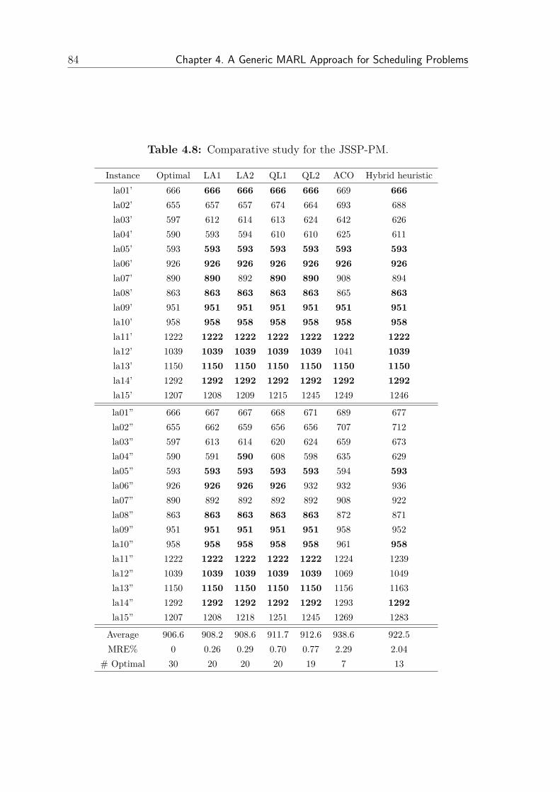
84 Chapter 4. A Generic MARL Approach for Scheduling Problems
Table 4.8: Comparative study for the JSSP-PM.
Instance Optimal LA1 LA2 QL1 QL2 ACO Hybrid heuristicla01’ 666 666 666 666 666 669 666la02’ 655 657 657 674 664 693 688la03’ 597 612 614 613 624 642 626la04’ 590 593 594 610 610 625 611la05’ 593 593 593 593 593 593 593la06’ 926 926 926 926 926 926 926la07’ 890 890 892 890 890 908 894la08’ 863 863 863 863 863 865 863la09’ 951 951 951 951 951 951 951la10’ 958 958 958 958 958 958 958la11’ 1222 1222 1222 1222 1222 1222 1222la12’ 1039 1039 1039 1039 1039 1041 1039la13’ 1150 1150 1150 1150 1150 1150 1150la14’ 1292 1292 1292 1292 1292 1292 1292la15’ 1207 1208 1209 1215 1245 1249 1246
la01” 666 667 667 668 671 689 677la02” 655 662 659 656 656 707 712la03” 597 613 614 620 624 659 673la04” 590 591 590 608 598 635 629la05” 593 593 593 593 593 594 593la06” 926 926 926 926 932 932 936la07” 890 892 892 892 892 908 922la08” 863 863 863 863 863 872 871la09” 951 951 951 951 951 958 952la10” 958 958 958 958 958 961 958la11” 1222 1222 1222 1222 1222 1224 1239la12” 1039 1039 1039 1039 1039 1069 1049la13” 1150 1150 1150 1150 1150 1156 1163la14” 1292 1292 1292 1292 1292 1293 1292la15” 1207 1208 1218 1251 1245 1269 1283
Average 906.6 908.2 908.6 911.7 912.6 938.6 922.5MRE% 0 0.26 0.29 0.70 0.77 2.29 2.04
# Optimal 30 20 20 20 19 7 13

Chapter 4. A Generic MARL Approach for Scheduling Problems 85
Therefore, the learning/optimization method proposed in this section is an offlinescheduling approach divided in two steps. First, a two-stage learning method isapplied to obtain feasible schedules, which can then be used as initial data for anoptimization procedure [Van Peteghem & Vanhoucke (2008)] during the second step.
The implemented learning method decomposes the problem following the assign-then-sequence approach. Therefore, we have two learning phases. During the firstphase operations learn what is the most suitable machine and during the secondphase machines learn in which order to execute the operations in order to minimizethe makespan. For this, each phase has a Q-Learning algorithm associated. As theprocess is being divided in two, we take into account the goal of each phase in orderto define the states and the possible actions.
In the first phase, where the learning takes care of the routing, we have anagent per operation being responsible for choosing a proper machine to execute itscorresponding operation. This machine has to be selected from the given set ofavailable ones, that is, the set of resources that can execute it.
This is not the case for the second phase, where the learning algorithm takes careof the sequencing and each operation already knows where it has to be executed, themain idea is to decide the order in which they will be processed on the machines.As it can be seen, this is what our basic approach (proposed in section 4.1) does,which means that in the second phase we will have an agent per resource, selectingoperations based on the quality of the solution.
What still needs to be defined is how to choose a proper machine for each oper-ation.
4.3.2 Example
Assuming that we have a small instance with 2 jobs and 3 machines, where J1 has2 operations and J2 has 3 operations, and these operations can be executed by thefollowing sets of machines, where each pair represents a possible machine and thecorresponding processing time:
J1O1
M1, 10
M2, 15J1O2
M2, 12
M3, 18

86 Chapter 4. A Generic MARL Approach for Scheduling Problems
J2O1
M1, 20
M3, 25J2O2
M1, 25
M2, 18J2O3
M2, 15
M3, 25
As mentioned in the description of the algorithm, the first learning phase takescare of the routing, meaning that the first step is to choose an appropriate machinefor each operation.
Let us assume that each operation can select the machine that will take careof its processing, the obvious decision will be to choose the fastest machine, whichmeans that J1O1 will select M1, because it only needs 10 times steps, while M2 willtake 15. If we repeat this process for each of the operations then the selection willbe as follows:
J1O1
M1, 10 X
M2, 15J1O2
M2, 12 X
M3, 18
J2O1
M1, 20 X
M3, 25J2O2
M1, 25
M2, 18 XJ2O3
M2, 15 X
M3, 25
From these operation-machine assignments it is possible to see that if all theoperations go for the fastest machine, then M1 will have to execute 2 operations,and machine M2 the remaining three operations, while M3 stays idle during thewhole process.
After performing the sequencing, a possible solution for the operation-machineassignment is shown in Figure 4.11, which results in a makespan Cmax = 63:
The optimal solution for this instance is shown in Figure 4.12, with a makespanCmax = 53.
This optimal solution responds to the following operation-machine assignment:
J1O1
M1, 10
M2, 15 XJ1O2
M2, 12
M3, 18 X
J2O1
M1, 20 X
M3, 25J2O2
M1, 25
M2, 18 XJ2O3
M2, 15 X
M3, 25

Chapter 4. A Generic MARL Approach for Scheduling Problems 87
Figure 4.11: Schedule for the operation - machine assignments using thefastest machine.
Figure 4.12: Optimal schedule for the example.
As can be seen, always taking the machine that will process the operations thefastest is not a good choice, as there are other important criteria that should beconsidered, for example, the workload of the machine.
That is why we use the end time of its corresponding operation on the selectedmachine as feedback signal for the agents. Of course its objective is to minimize theend time of the operation, that is, the time when the machine finishes executing theoperation.
Once a feasible schedule has been found, the mode optimization procedure canbe executed. This procedure will be described in the next subsection.
4.3.3 Mode Optimization Procedure
The mode optimization procedure [Van Peteghem & Vanhoucke (2008)] is a forward-backward procedure which tries to shift a schedule to the left (as much as possible) inorder to minimize the makespan. It is executed once a feasible schedule is obtained,and we refer to it as the second step of the approach.

88 Chapter 4. A Generic MARL Approach for Scheduling Problems
The forward-backward procedure can be summarized as follows:
• Order the operations according to their end times (the time when they end inthe schedule received as input).
• Taking into account the previous ordering, for each operation, choose the ma-chine that will finish it first (shortest end time, not shortest processing time).The result is a backward schedule.
• Repeat steps 1 and 2 to obtain a forward schedule.
Once the mode optimization is executed, the quality of the solution is taken intoaccount to give feedback to the agents of the learning phases.
Example 4: Let us say that after executing the learning step we obtain the scheduleshown in Figure 4.13.
Figure 4.13: Feasible schedule obtained by the learning step.
Applying the Mode Optimization Procedure to this schedule, the first step is toorder the operations according to their end times, that will give us the followingordering: J2O3, J2O2, J2O1, J1O2 and J1O1. Taking into account this ordering,the operations will choose a machine to execute it, basing the decision on the possibleend time (according to the data given in subsection 4.3.2).
For example, J2O3 can start choosing because it was the first operation in theordering, according to the data of the example the machines that can execute itare M2 for 15 time steps or M3 for 25 time steps, obviously the best choice is M2,meaning that M2 will be busy between time 0 and 15.
J2O3
M2, 15 (0− 15) X
M3, 25

Chapter 4. A Generic MARL Approach for Scheduling Problems 89
Then, the next operation on the ordered list makes a choice, in this case J2O2
can choose between M1 for 25 time steps and M2 for 18. As this is the secondoperation of J2 being scheduled, it can not start until the previous operation of thesame job is finished, which means that its earliest starting time will be 15 (which isthe time when J2O3 is finished), the possible end times are then 40 on M1 (15+25)and 33 on M2 (15+18), being the best choice M2, which will be occupied from 15to 33.
J2O2
M1, 25 (15− 40)
M2, 18 (15− 33) X
When an operation from another job chooses a machine, it has to respect thisbusy times but it can search for an available slot of the size of the time it requires.Once all the operations are scheduled, a backward schedule is obtained, which willlook as shown in Figure 4.14.
Figure 4.14: Backward schedule.
This process is repeated once again, in order to find a forward schedule, an-alyzing the backward schedule it will give us the following operation ordering:J2O1, J2O2, J1O1, J1O2, J2O3. After repeating the choosing procedure, a forwardschedule like the one shown in Figure 4.15 is obtained.
It is possible to see that we obtain a makespan Cmax = 53, and initially westarted with a schedule where Cmax = 80.

90 Chapter 4. A Generic MARL Approach for Scheduling Problems
Figure 4.15: Forward schedule.
The Learning / Optimization approach can be summarized as follows:
Algorithm 2 Learning/Optimization algorithm for the FJSSPStep 1 - Learningfor each operation dochoose a machine
end forwhile there are operations to execute dofor each machine with queued operations dochoose operation to executeupdate queues of the system
end forend whileStep 2 - Execute the Mode Optimization Procedure
4.3.4 Experimental Results FJSSP
Several experiments were performed using benchmark problems proposed in [Brandi-marte (1993)] (see subsection 2.6.1). The results of this approach were reportedin [Martínez et al. (2011)].
The combination of parameters used for the experiments was γ = 0.8 and ε = 0.1,together with a discount factor α = 0.1. The algorithm was executed for 10,000iterations.

Chapter 4. A Generic MARL Approach for Scheduling Problems 91
4.3.5 Comparative Study
Table 4.9 shows a comparative study between the proposed approach and someresults reported in the literature. LB is the Lower Bound for each instance, takenfrom the original Brandimarte data [Brandimarte (1993)]. The algorithms used tocompare our method (QL) are:
• GA: Genetic Algorithm [Pezzella et al. (2008)], algorithm integrating differentstrategies for generating the initial population, selecting the individuals forreproduction and reproducing new individuals.
• ACO: Ant Colony Optimization [Lining & Chen (2010)], it provides an effec-tive integration between the Ant Colony Optimization model and knowledgemodel.
• GEN: Abbreviation of GENACE, an architecture proposed in [Ho et al. (2007)]where an effective integration between evolution and learning within a randomsearch process is proposed.
• Brand: Tabu Search [Brandimarte (1993)], a hierarchical algorithm for theflexible job shop scheduling based on the tabu search metaheuristic.
Table 4.9: Experimental Results FJSSP.
Inst. LB GA ACO GEN Brand QLMk01 36 40 39 40 42 40Mk02 24 26 29 29 32 26Mk03 204 204 204 204 211 204Mk04 48 60 65 67 81 66Mk05 168 173 173 176 186 173Mk06 33 63 67 67 86 62Mk07 133 139 144 147 157 146Mk08 523 523 523 523 523 523Mk09 299 311 311 320 369 308Mk10 165 212 229 229 296 225
Table 4.10 shows the mean relative errors in % (MRE) of the different approachesused to compare our method with respect to the best-known lower bounds.

92 Chapter 4. A Generic MARL Approach for Scheduling Problems
Table 4.10: MRE: Mean relative errors
GA ACO GEN Brand QLMRE 17,53 22,16 23,56 41,43 19,69
From the tables (4.9 and 4.10) we see that the proposed approach is able to findthe best reported value for several instances (Mk01-Mk03, Mk05, Mk08). For theinstances Mk04, Mk07 and Mk10 the genetic algorithm is better. For the instancesMk06 and Mk09 the proposed algorithm is able to yield better results.
The cases in which our algorithm did not find the best solutions where instancesfor which a proper machine assignment was not found, probably caused by thefact that multiple machines with similar processing times can perform the sameoperation.
4.4 Reinforcement Learning for Online Scheduling
After dealing with three different scheduling problems where all the information wasknown beforehand, we switch to a completely different scenario, an online schedulingproblem which is depicted in Figure 4.16 (see Section 2.8). In this case the solutionmethod will be Learning Automata, described in subsection 3.4.3.
Figure 4.16: A two-stage chemical production plant. For both producttypes P1 and P2, there are two parallel machines at the first stage. At thesecond stage of the process, there are also two parallel machines.
4.4.1 Learning Automata for Stochastic Online Scheduling
In order to apply LA to a scheduling problem we need to define the actions of theagents and the rewards. We define an action of the LA as submitting a job to

Chapter 4. A Generic MARL Approach for Scheduling Problems 93
one of the parallel machines. Therefore, for the problem described we will have 6agents, one in each decision point, which means that two agents receive productorders P1 and P2 and decide which ‘stage-1’ machine will be used. The other fouragents receive partially processed jobs from a ‘stage-1’ machine M1− and send themto a ‘stage-2’ machine M2−. Note that the agent cannot wait to submit a job andcannot stop a job preemptively. In other settings these could be added as extraactions [Martínez et al. (2010)a].
When a job j is completely finished, the two agents that decided the path ofthat job are notified. Based on the completion time Cj and the release times rj forboth stages a reward r ∈ 0, 1 is created, see Equation 4.4. Note, (i) completiontime is the time at which the job has finished both stage 1 and stage 2, and (ii)release times are the times at which the job starts stage 1 or stage 2 depending onthe agent.
r =
0 if F > Favg,
1 otherwise,(4.4)
where the flowtime F = Cj−rj and Favg is the average flowtime over the last n jobs.The larger n, the more accurate the LA’s belief of the average flowtime of the jobs.The smaller n the faster the LA will adapt its belief of the average flowtime whenfor example a machine breaks down or the performance of a machine increases.
4.4.2 WSEPT Heuristic for Stochastic Online Scheduling
To the best of our knowledge, there is no good approximation algorithm for schedul-ing problems that are online, stochastic and multi-stage at the same time. For thesingle-stage case, there exists a very good heuristic: Weighted Shortest ExpectedProcessing Time (WSEPT) [Megow et al. (2006)].
This heuristic works as follows: orders are arriving over time and must be pro-cessed by one out of several parallel machines. The objective is to reduce the totalweighted completion time (∑j wjCj, for all jobs j). Each time an order arrives, theWSEPT rule submits the job to the machine that is expected to finish it first. Tothis end it polls each machine for its current expected makespan (including the newjob). If, for example, all jobs have equal expected processing time, and each machinethe same average speed, then the expected makespan is the queuelength (includingthe currently processed job if any). In [Megow et al. (2006)] lower bounds on thetotal weighted completion time (∑j wjCj) are given for the WSEPT heuristic.

94 Chapter 4. A Generic MARL Approach for Scheduling Problems
In the next section we will compare the WSEPT and the Learning Automata ina simple single-stage scheduling task.
4.4.3 Experimental Results
4.4.3.1 WSEPT Heuristic versus Learning Automata
We ran some experiments on single-stage scheduling with N = 4, 5 or 6 identicalmachines. One scheduler receives a sequence of jobs. The joblengths are generatedby an exponential distribution with average µ = 100. The identical machines haveunit processing speed si = 1, for i = 1, . . . , N . I.e. a machine needs 100 timestepsto process an average job.
To make sure the system can actually handle the load, we set the probability ofcreating a job at any timestep to 95% of the total processing speed divided by theaverage job length: 0.95∑i si/µ. In this setting, all jobs have unit weight wj = 1.
We tested the following agents on the same sequence of orders:
RND: uniformly distributes the jobs over all machines,
WSEPT: uses the WSEPT heuristic as described in Section 4.4.2,
LA: a Learning Automaton as described in Section 4.4.1 with α = β = 0.02.
Results: The experiments showed that the LA clearly performs better than theRND scheduler, and WSEPT outperforms LA [Martínez et al. (2010)a]. Note thatthe heuristic approach uses a lot more information which LA cannot access. Thelength of the queues over time show that WSEPT balances the load better: queuesare 4 to 5 times shorter. On the other hand, the total weighted completion time(∑j wjCj) does not show huge differences between WSEPT and LA (in the order of0.001 to 0.01 time units).
Although the WSEPT heuristic outperforms the Reinforcement Learning ap-proach, it requires access to more information and only works in single-stage load-balancing problems. This is why in the next section, we test LA in the multi-stagesetting described at the beginning of Section 4.4.1.
4.4.3.2 Multi-Stage Scheduling
In this case we look at two slightly different settings, which are summarized in Ta-ble 4.11. Setting 1 is adopted from [Peeters (2008)]. In both cases, the average

Chapter 4. A Generic MARL Approach for Scheduling Problems 95
joblength is 100 and the jobrate is 1/45 for both product types P1 and P2. The per-formance is measured by the total flowtime of the jobs through the entire processingchain.
Table 4.11: Processing speeds of all machines for two different settings.
Machine M11 M12 M13 M14 M21 M22 M23 M24
Speed setting 1 3.33 2 1 1 3.33 1 1 1Speed setting 2 3.33 2 10 10 3.33 1 1 1
In order to compare the results, a random strategy for dispatching the jobs wasalso implemented under these settings. Figure 4.17 shows how the queues of themachines grow when following this strategy, where each color represents a machine(8 in total).
Figure 4.17: Queues of the machines when following the random strategy.
The first type of LA we tested was Linear Reward-Inaction LA (LR−I). Aftersome time, the queues started growing indefinitely. This was caused by some au-tomata converging prematurely to a pure strategy, i.e. they end up selecting thesame action forever. This is due to the fact that LR−I never penalizes bad actions(β = 0). Although this may be favorable for many RL problems, it will almost neverbe for load-balancing. The only obvious exception is when one machine is able toprocess all jobs before any new order arrives.

96 Chapter 4. A Generic MARL Approach for Scheduling Problems
Figure 4.18 shows the queues of the machines when using Linear Reward-InactionLearning Automata.
Figure 4.18: Queues of the machines when using Linear Reward-Inaction.
The LR−εP generated better and better results when ε was increased. Finally,when ε = 1 we have LR−P , where penalty and reward have an equally large influenceon the probabilities. This gives the best results. Figure 4.19 shows the queues ofthe machines when using learning automata under the reward penalty strategy.
Figure 4.19: Queues of the machines when using LR−εP .
Figure 4.20 shows the results in terms of the amount of queued jobs at the end

Chapter 4. A Generic MARL Approach for Scheduling Problems 97
of the process (25000 iterations), while Figure 4.21 shows the amount of jobs thatwere executed also after the total number of iterations.
Figure 4.20: Queued jobs at the end of the process.
Figure 4.21: Total number of jobs executed at the end of the 25000iterations.
Different combinations of values for the parameters α and β were studied. Theseparameters determine the learning speed, and the best combination for this problemwas 0.01. Table 4.12 shows the average policy for each of the six agents. For example,the fourth agent receives jobs partially finished by machineM13 and distributes themover M23 and M24.

98 Chapter 4. A Generic MARL Approach for Scheduling Problems
The second setting shows that the agents take into account the time needed fora job to go through all stages. Machines M13 and M14 are 10 times faster as in thefirst setting. This does not increase the total system capacity, since the machines inthe second stage would create a bottleneck. The result is that the first two agentsstill favor M11 and M12, but slightly less. For example, the first agent in Table 4.12distributes 71% of the load on M11 in the second setting, as opposed to 74% in thefirst setting.
Table 4.12 shows the average probabilities of all agents through an entire simu-lation.

Chapter 4. A Generic MARL Approach for Scheduling Problems 99
Tab
le4.12:Av
erageprob
abilitie
sof
alla
gentsthroug
han
entir
esim
ulation.
Machine
M11
M13
M12
M14
M21
M22
M23
M24
M21
M22
M23
M24
Setting1
.74
.26
.69
.31
.76
.24
.50
.50
.77
.23
.50
.50
Setting2
.71
.29
.61
.39
.77
.23
.50
.50
.78
.22
.50
.50

100 Chapter 4. A Generic MARL Approach for Scheduling Problems
4.4.4 Discussion
The following advantages of LA make them very applicable in difficult schedulingscenarios:
• They can cope with unknown joblengths, unknown future jobs and unknownmachine speeds.
• The decisions based on the probability distribution and the updates of thosedistribution are straightforward. They can be performed in a minimum of timeand require only very limited resources.
• No heuristics or additional information is needed.
The performed experiments show that LA can learn processing capacities ofentire downstream chains. Note however that the rewards are delayed. Whilewaiting for a submitted job to be finished, other jobs must already be scheduled.In our scheduling problem, this is not a problem for the LA. When more stageswould be added to the system, the LA could be equipped with so-called eligibilitytraces [Castillo & Roberts (2001)].
Since LA are very adaptive, and will not converge to pure strategies with LR−P ,they are able to adapt to changes in processing speed, such as machine break downs.
Finally, when applying any randomization technique (such as LA) to balance aload, one is always better off with many short jobs than very few long ones (cf. thelaw of large numbers).
4.5 SummaryIn this chapter we first introduced what we call the basic learning algorithm, whichwas initially defined for the job shop scheduling problem and later on adapted inorder to solve the version with parallel machines and the flexible job shop scheduling.The learning method implemented was a Q-Learning algorithm, for which differentfeedback signals were studied. This QL algorithm was easily adapted and combinedwith other techniques in order to satisfy the extra constraints of the more challengingscenarios. In all the cases the results were compared with those reported in theliterature by other approaches. For the online scheduling problem we used LearningAutomata in order to learn how to distribute the incoming orders of two types ofproducts among parallel machines. Experiments were developed using the three

Chapter 4. A Generic MARL Approach for Scheduling Problems 101
possible update schemes. The results of the experiments showed that the LR−Pscheme was able to yield better results. In the following chapter we will presentsome of the more common sources of uncertainty in scheduling and introduce theconcept of robustness.


Chapter 5
Uncertainty and Robustness inScheduling
In real-world applications of Linear Programming, one cannot ignore thepossibility that a small uncertainty in the data can make the usual
optimal solution completely meaningless from a practical viewpoint.- [Ben-Tal & Nemirovski (2000)]-
In real world environments scheduling can not be seen as a problem where all theinformation is known beforehand. For example, manufacturing scheduling is subjectto constant uncertainty in its environment, where the probability of a schedulebeing executed exactly as it was planned is usually very low. In this chapter wesummarize the more common sources of uncertainty in scheduling, and differenttypes of approaches to deal with these uncertainties are studied. These approachescan be classified as proactive or reactive. We will go into more detail in the proactivetechniques, as the approach we propose in the next chapter is based on this idea.The concept of robustness is defined and different metrics to measure how robust aschedule is are described.
103

104 Chapter 5. Uncertainty and Robustness in Scheduling
5.1 Uncertainty in SchedulingDuring the scheduling process machines can break down, operations can take longerthan expected, new orders can arrive, the priority of some orders might change, andall these disruptions will eventually make the original schedule fail, causing delaysin the delivery of the products (due dates might be violated), increasing the idletimes of the machines and the staff, among many other consequences.
Therefore, in real environments it may not be useful to spend significant effortsto produce optimal solutions, since the optimality is achieved only if the solutioncan be executed as planned. On the contrary, as noted in [Policella (2005)], “a sub-optimal schedule that contains some built-in flexibility for dealing with unforeseenevents, might provide useful characteristics for the execution. Hence, the efficiencyof the scheduling techniques employed will depend on the degree of uncertainty of thescheduling information provided at the beginning”.
Figure 5.1 shows another graphical representation (more detailed than Figure2.1) of the supply chain environment where scheduling operates.
Figure 5.1: Scheduling Environment, taken from [Gao (1996)].
The input of this chain is composed of a set of demands or orders from internaland/or external customers, these demands are given to the scheduler, who providesa schedule to the shop floor for execution. The shop floor uses internally produced

Chapter 5. Uncertainty and Robustness in Scheduling 105
materials, and also receives part of them from outside suppliers, producing the finalproducts that are stored in a warehouse until they are delivered to the customerswho ordered them [Gao (1996)].
As it can be seen, scheduling works at a very low level inside production man-agement, but it is in this level where the shop floor strategy is planned, that is whyit is very important to come up with schedules that will allow to accomplish thedesired objective and satisfy the customers.
One of the major existing problems in scheduling is that plans or schedules thatare good on paper often do not perform well in practice, due to the previously men-tioned uncertainty in the environment. In the search of optimal solutions machinesare constantly working and the operations are executed as soon as possible in orderto meet the due dates and minimize objectives like the makespan or the tardiness.That is why most of the time we are faced with non-delay schedules, which are goodin practice as long as unexpected events do not occur.
It is important to say that even though the presence of idle times is usuallyconsidered as bad when scheduling, it is good in performance, because it is whatkeeps delays from propagating [Cohn (2007)].
Some of the more common sources of uncertainty at the operational level are:
• Machine breakdowns;
• Uncertainty in the processing times of the activities;
• Unexpected arrival of new orders, some of them with high priority;
• Cancellation or modification of existing orders;
• Modification of release and/or due dates.
In this dissertation we will focus on the first two, Machine breakdowns andVarying activity duration. One way to deal with such disruptions is by generat-ing robust schedules [Davenport et al. (2001)], that is, schedules with the ability tosatisfy performance requirements predictably in an uncertain environment [Le Pape(1991)]. In the next section we will introduce the concept of robustness and we willanswer some important questions, such as how to measure how robust a schedule is,and how to incorporate robustness in our solutions.

106 Chapter 5. Uncertainty and Robustness in Scheduling
5.2 RobustnessIn many decision processes it is common that solutions with a certain level of robust-ness are required in order to maintain their feasibility in settings with incompleteor imprecise data. Solutions should tolerate a certain degree of uncertainty duringexecution, in other words, they should be able to absorb dynamic variations in theproblem.
We often talk about robust schedules, but there are several questions that haveto be answered in order to truly capture the meaning of robustness, for example:
• how is robustness defined?
• how can we measure how robust a schedule is?
• how to incorporate robustness in the schedules?
The robustness of a schedule is a way to characterize its performance. In [Billautet al. (2008)], a schedule is classified as robust if its performance is rather insensitiveto data uncertainties. Another definition of robust schedule is given in [Leon et al.(1994)], in this case it is defined as a schedule that is insensitive to unforeseenshop floor disturbances given an assumed control policy. In other words, robustscheduling tries to protect the schedules from stochastic events.
The development of robust optimization was initiated by Soyster in 1973 [Soys-ter (1973)]. This approach has been extensively studied and extended, as it wasconsidered too conservative, in the sense that it produces solutions that give up toomuch of optimality for the nominal problem in order to ensure robustness [Bertsimas& Sim (2004)].
After this initial work some other models were proposed, see for example [Ben-Tal & Nemirovski (2000)], [Bertsimas & Sim (2004)] and [Lui Cheng (2008)]. In allof them the main concern is how to make the schedules more robust without loosingtoo much in optimality.
5.2.1 Measuring Robustness
A property such as robustness is easy to define, but difficult to measure in a quanti-tative manner. In [Sabuncuoglu & Goren (2009)] the authors present a deep studythat shows how different approaches focus on different objectives and as a conse-quence, the way of measuring robustness is not always the same.

Chapter 5. Uncertainty and Robustness in Scheduling 107
In the literature, the following metrics are commonly used to measure the ro-bustness of a schedule:
1. deviation from the original schedule;
2. the real cost incurred by the implementation of the schedule;
3. stability - relatively to a performance criterion;
4. number of changes required to ‘fix’ the solution.
The first two measures were proposed in [Gao (1996)], according to the author,the deviation from the original schedule can be computed by analyzing the differencebetween the planned makespan and the actual makespan. In the second case costscan be associated, for example, to tardiness, meaning that there is a penalty pertime unit scheduled over the due date. Or costs could be associated to resourceidleness, which means that there is a penalty for each time unit that the resourcewas kept idle.
In the case of the stability (third metric), we can say that it is quite similar tothe first metric. According to its definition in [Billaut et al. (2008)], stability is ameasure of the sequence difference between the two schedules, which in other wordsis how deviated is the actual schedule from the original one.
For the last metric, which was introduced in [Gomes (2000)], the intuition behindrobustness is the following: given a set C of changes to the initial formulation of theproblem instance, a solution A is more robust than a solution B with regard to theset C if the number of changes required to fix solution A is less than the number ofchanges required to fix solution B.
There are different approaches that can be used in order to deal with uncertaintyand robustness in scheduling, either finding solutions which adapt dynamically tochanges or incorporating available knowledge about possible changes to the solution[Herroelen & Leus (2005)]. These approaches will be explained in detail in the nextsection.
5.3 Proactive vs. Reactive ApproachesAccording to the literature, there are two ways to deal with uncertainty in schedul-ing environments, using proactive approaches (also called predictive) or reactive ap-proaches.

108 Chapter 5. Uncertainty and Robustness in Scheduling
The goal of proactive scheduling is to take into account possible disruptionswhile constructing the original predictive schedule. This allows to make the pre-dictive schedule more robust, because it has some statistical knowledge of uncer-tainty [Davenport & Beck (2000)].
Proactive scheduling has also been defined as techniques that seek to produce anoff-line schedule that is robust to execution time events [Beck & Wilson (2007)]. Theutility of this type of approach depends on whether the uncertainty can be quantifiedin some way (like knowing the mean time between failure for the machines etc). Ifthe information is available, it can be used by proactive techniques. If however, thedegree of uncertainty is very high, a more reactive approach is needed.
Reactive scheduling involves revising or reoptimizing a schedule when an un-expected event occurs. Completely reactive approaches are based on up-to-dateinformation regarding the state of the system [Davenport & Beck (2000)]. Decisionsare made in real time, based on priority dispatching rules, as no predictive scheduleis given to the shop floor. These approaches are used when the level of disturbancesis always significant or when the data are known very late, making the computationof predictive schedules impossible [Aloulou & Portmann (2005)].
Figure 5.2 shows a graphical representation of the properties of both types ofapproaches.
Figure 5.2: Predictive vs. Reactive Scheduling
Sometimes both points of view are combined and the combination is calledpredictive-reactive approaches. In this case a predictive schedule is generated with-out considering possible perturbations. Then, a reactive algorithm is used to main-tain the feasibility of the schedule and/or improve its performances, see for exam-

Chapter 5. Uncertainty and Robustness in Scheduling 109
ple [Church & Uzsoy (1992)], [Vieira et al. (2003)] and [Aloulou & Portmann (2005)].For further reading and a thorough overview on these types of approaches we referto [Sabuncuoglu & Goren (2009)].
5.3.1 Reactive Approaches
Based on the description provided in the previous section, we can conclude thatreactive scheduling aims at finding approaches to (ideally) optimally react to dis-ruptions after they occur. According to the literature, the reaction generally takesthe form of either modifying the existing initial schedule (repairing), or generatinga completely new schedule from scratch [Sabuncuoglu & Goren (2009)].
When the unexpected event is a breakdown, the simplest way to solve a reschedul-ing problem is to keep the processing order of the preschedule, but delay the pro-cessing when it becomes necessary. This kind of rescheduling is usually called ‘sim-ple rescheduling’ [Jensen (2001)], and it has been used for example in [Leon et al.(1994)].
Another type of approach is the one presented in [Wu et al. (1999)]. In this workthe author developed a decomposition method that partitions job operations intoan ordered sequence of subsets. This decomposition identifies and resolves a ‘crucialsubset’ of scheduling decisions through the use of a branch-and-bound algorithm.The computational experiments were conducted under a wide range of processingtime perturbations.
Another reactive strategy is list scheduling, which is applied in [Lambrechtset al. (2010)]. In this type of approach a random precedence feasible priority listis used as starting point, or also a scheduled order list that allows to reschedulethe activities in the order dictated by the schedule, while taking into account thenew, reduced resource availabilities. More specifically, when a disruption occurs attime t a priority list L is created including the activities that are not yet completed,ordered in a non-decreasing order of their baseline starting times. The priority list isdecoded into a feasible schedule using a modified serial schedule generation schemeand taking into account the known resource availabilities up to the current timeperiod. This idea is also applied for example in [Wauters et al. (2010)].
The approaches presented in [Wauters et al. (2010)] and [Kaddoum (2011)] willbe briefly explained at the beginning of next chapter, as they will be used to comparethe results of our approach.

110 Chapter 5. Uncertainty and Robustness in Scheduling
5.3.2 Proactive Approaches
In order to obtain robust schedules, an intuitive approach consists in adding someform of redundancy to the solution during the scheduling process. Figure 5.3 showsan example of two different solutions for the same scheduling problem. Schedule a) isthe classical example of a non-delay schedule, where the objective is to optimize theresource utilization, that is why each activity starts as soon as its predecessor ends.On the other hand, schedule b) presents some idle intervals between the executionof the different activities. For example, activity ‘b’ does not start immediately afteractivity ‘a’ is finished. This approach allows to tolerate some changes in the originalproblem like delay in the activity processing and machine breakdowns. At the sametime, by introducing redundancy the resource utilization is reduced, which meansthat objective functions like minimizing the makespan or the tardiness will also beaffected. Therefore, the main goal of the redundancy-based approaches is to findout how much redundancy is needed and how this redundancy has to be distributedover the whole solution.
a
time
time
b d
c e f g
a b d
c e f g
a
time
time
b d
c e f g
a b d
c e f g
new resource
breakable resource
a
time
time
b d
c e f g
a b d
c e f g
Figure 5.3: Increasing robustness by adding redundancy. Schedule b) isconsidered more robust than schedule a).
In this dissertation we focus on proactive approaches, more specifically on tech-niques that deal with uncertainty by inserting some form of redundancy (typicallyextra time) in the schedule. These techniques will be referred to as slack-basedtechniques and are explained in detail in the next section.

Chapter 5. Uncertainty and Robustness in Scheduling 111
5.4 Slack Based Techniques
According to the literature, the main idea behind slack-based techniques is to provideeach activity with some extra execution time so that some level of uncertainty canbe absorbed without rescheduling. In order to do that, these techniques base theirbehavior on existing knowledge about failures of the machines, for example: themean time between failures, or the mean down time of a resource. In this sectionwe will describe three slack-based techniques: Temporal Protection, Time WindowsSlack and Focused Time Windows Slack.
5.4.1 Temporal Protection
Temporal Protection, first proposed by Chiang and Fox [Chiang & Fox (1990)], isa technique that is based on the idea of predictively building a schedule taking intoaccount previous knowledge of uncertainty.
Resources that have a non-zero probability of breakdown are identified as break-able resources. The duration of all the activities requiring breakable resources isextended in order to provide extra time to cope with the breakdowns and thescheduling problem with protected durations is then solved with standard schedulingtechniques [Gao (1996)].
Let us show an example based on the one presented in [Davenport et al. (2001)].Figure 5.4 depicts two activities, A and B, which are sequenced on a breakableresource. The white part of the boxes represents the original processing time ofthe activities, and the gray part represents the extra time added by the temporalprotection technique. If the resource breaks down while activity A is being executed,the extra time can be used to absorb the breakdown, or part of it. If it does nottake longer than the available protection then the rest of the schedule will remainas planned. If it lasts longer, then some adjustment is needed in order to keepexecuting the rest of the activities (rescheduling, right shifting, etc). If there are nobreakdowns while activity A is executed then activity B can start earlier, meaningthat the slack provided by the temporal protection to activity A can be used byactivity B.
One important point when using the temporal protection, or any other slack-based technique is to decide the amount of extra time that will be added to eachactivity. Too much protection will end up with a poor quality schedule, but a highly

112 Chapter 5. Uncertainty and Robustness in Scheduling
Figure 5.4: Example of two consecutive operations which are executedon a breakable resource. The white part of each box represents the originalprocessing time of the operation and the gray part represents the extratime added by the temporal protection technique.
robust one. Too little protection will result in a poor quality schedule execution ifa breakdown occurs. The approach presented in [Gao (1996)] extends the durationof each activity requiring a breakable resource in the following way:
pijext = pij + pijF×D (5.1)
Where pij is the original processing time of the activity, F represents the ex-pected time between machine failures and D is the duration of the breakdown orinterruption.
pijext is the extended processing time, by adding the total expected down time tothe uninterrupted processing duration. pij
Fgives the expected number of breakdowns
during the processing of an activity. pij
F×D represents the duration extension caused
by the machine breakdowns.
Figure 5.5 shows two schedules, on top we have a non-delay schedule, whereall the operations are executed as soon as the resources become available. In thiscase, the resource responsible for executing operations a, b and d is considered asbreakable, which means that these three operations will be ‘protected’ by receivingsome extra execution time.
It is important to remember that if breakdowns do not occur, or if they do occur,but take less time than the slack time added, operations that are scheduled after a‘protected’ operation can start their processing earlier.

Chapter 5. Uncertainty and Robustness in Scheduling 113
Figure 5.5: Example of schedule where a breakable resource has threeoperations scheduled.
5.4.2 Time Window Slack
If we analyze the way the Temporal Protection technique uses to add the slack times,we will notice that there are situations where it will not be possible to ‘share’ slackbetween activities, even if there are no breakdowns. For example, the environmentshown in Figure 5.4 is extended in Figure 5.6 by adding a third operation C, whichis being executed on a non-breakable resource, meaning that it does not have extratime associated. According to the ordering constraints activity B must be executedafter activity C is finished, which means that the earliest start time for B is the endtime of C.
In order to avoid such situations, where the slack time added can not be usedby upcoming operations, the Time Window Slack (TWS) approach was proposedin [Davenport et al. (2001)]. In this approach the authors change the way of addingslack to the operations so that they make sure that the schedule has sufficient slacktime for each activity.
It is important to mention that the required slack for an activity under TWSis considerably longer than the duration extension in temporal protection. Morespecifically, the amount of slack on each activity is equal to the sum of the durationsof all the expected breakdowns of resource R, and this is mainly due to the fact thatauthors expect the slack of all the activities on each resource to be shared [Davenportet al. (2001)].
Equation 5.2 shows how the slack is calculated in this approach. In this equationpij represents the duration of the activity, µtbf (R) is the mean time between failures

114 Chapter 5. Uncertainty and Robustness in Scheduling
Figure 5.6: Example where the slack time added by the temporal pro-tection method can not be used by the next activity on the same machinedue to ordering constraints.
on resource R and µdt(R) represents its mean down time (breakdown duration). Theset of activities that can be executed on resource R is given by actsR.
slackA ≥∑B∈actsR
pijµtbf (R) × µdt(R) (5.2)
Figure 5.7 shows how the TWS method adds extra execution time on everyoperation, assuming that the slack of all the activities on each resource will beshared.
Figure 5.7: Adding slack time under the Time Windows Slack method.
In short, when using temporal protection, the expected down time of each re-source is divided into the different operations and the slack times are added based

Chapter 5. Uncertainty and Robustness in Scheduling 115
on this value. When using TWS, the slack time is equal to the sum of the durationsof all the expected breakdowns on resource R, because the slack is expected to beshared.
5.4.3 Focused Time Window Slack
The Focused Time Window Slack (FTWS) approach was also proposed in [Daven-port et al. (2001)]. In this approach, the placement of activities in the schedulinghorizon is taken into account in order to decide if some slack time will be needed.The authors use uncertainty statistics in order to focus the slack in parts of theschedule that are more likely to need it in order to deal with an unexpected event.
For example, they consider the scenario where a new machine can arrive to thesystem, in this case it will not make sense to make the schedule more robust at thebeginning, as this machine is new and it could take some time before it can breakdown.
The slack for the activities is calculated as a function of the probability that abreakdown will occur before or during its execution. Which means that the decisionon whether to add slack or not is based on known distributions.
Figure 5.8 extends the example shown in Figure 5.5 by considering the use ofa newly bought machine. In this case slack is added to the operations that arescheduled on this machine after a specific amount of time, for example, operation cdoes not receive extra execution time, as it is the first operation being executed bythe new machine, and it is not supposed to fail so fast.
Figure 5.8: Adding slack time using the Focused Time Windows Slackapproach.

116 Chapter 5. Uncertainty and Robustness in Scheduling
5.4.4 Discussion about the slack-based techniques
In general, all these slack-based methods base their behavior on the data they re-ceive about the uncertainty, but what if something happens on a machine wherebreakdowns are not expected? Consider again the example of the newly boughtmachine, a very fast one which is not considered as breakable, therefore, several op-erations are scheduled there, because it is a more reliable resource. If that machinefails, the schedule is not prepared to deal with the disruption, as it was a breakdownimpossible to forecast. This leads us to the following question:
Is it possible to construct more robust schedules without looking at the proba-bility distributions of the unexpected events as the only source of information?
In the next chapter we propose a new slack-based approach which does notrely on the probability distributions as the only source of information. It worksby analyzing something we call ‘criticality’ of the machines and/or the jobs andthe main objective is to add slack times in those parts of the schedule which areconsidered to be critical, or more likely to need extra execution time.
5.5 SummaryIn this chapter we presented some of the more common sources of uncertainty inscheduling, as well as the concept of robustness and different methods that canbe used in order to construct more robust schedules. We focused on proactiveapproaches, mainly slack-based techniques, as the approach we will propose in thenext chapter is based on this idea. These slack-based techniques work by addingextra execution time to the operations in order to absorb some level of uncertaintywithout having to reschedule. The next chapter will also introduce we will explainhow some new instances of the flexible job shop scheduling were generated in orderto introduce some levels of uncertainty.

Chapter 6
Scheduling under Uncertainty
Robust approaches aim at building solutions able to absorb some level ofuncertainty without rescheduling
- [Davenport & Beck (2000)] -
In order to address the uncertainty problems described in the previous chapter,the research described in this chapter will be divided in two parts. First, we willpresent a stochastic version of the flexible job shop scheduling, for which we alreadyshowed the results in the deterministic scenario. We describe the process of creatingnew instances and the results obtained are compared with the ones reported by otherstate of the art methods in terms of tardiness and makespan. In the new instances,release and due dates are added to the jobs, and perturbations are added to themachines.
In the second part we introduce a new proactive approach based on the ideaof the slack-based techniques presented in Chapter 5. This approach focuses onadding slack times in the critical parts of the schedule by taking into account thecriticality of the machines and the jobs, yet trying not to increase the makespantoo much. It also allows the user to decide on the level of robustness to includein the schedule construction process. Some examples demonstrate how this works,together with graphical representations (gantt charts) of the solutions. The lastpart of the chapter is concerned with the application of the approach to a real worldcase.
117

118 Chapter 6. Scheduling under Uncertainty
6.1 Deterministic Case with Known DisruptionsThere are cases when it is known beforehand that a specific machine will be subjectto maintenance during some amount of time, and this will interrupt the executionof the production process. In this case there are two possibilities, if the environmentis like the job shop scheduling, and the affected machine is the only one that canperform specific operations, then the only choice is to wait until it becomes availableagain. If parallel machines are available, meaning that operations can be executedby different machines, another resource can take over. It will be up to the algorithmto decide whether it is better to wait for the machine to become available or to sendsome operations to a parallel resource and possibly affect the schedule. Sometimes itwill be better just to wait for the machine to come back from maintenance, becausethe other possible machines have too many jobs in the queue.
This is a particular case that can be taken into account in our approach. If thereis some extra information about maintenances on the machines (which are alsoconsidered as perturbations), the user can add it to the problem instance, and thealgorithm will take it into account when constructing the solution. This informationcan be added to the instance in the following way:
• one line with the string #Perturbations, which indicates that from that pointon different perturbations will be listed.
• the second line has only one number, which represents the total amount ofperturbations that will be included.
• one line per perturbation indicating:
1. id of the perturbed machine
2. start time of the perturbation
3. duration of the perturbation
Figure 6.1 shows how the information will look like after being added to thescheduling instance. In this case two perturbations are included, the first one willbe on machine M1 and will happen at time step 23, with a duration of 4 time steps.The second one will occur on machine M2 at time step 45 and will last for 8 timesteps.
Once this information has been included in the problem instance, the agents willtake it into account when choosing their actions. In the case where the operations do

Chapter 6. Scheduling under Uncertainty 119
Figure 6.1: Adding scheduled maintenances to the instances.
not have execution alternatives the duration of the perturbation will just be addedto the processing time of the operation being processed on the resource when theperturbation (maintenance) starts.
In the case where multiple machines can execute one particular operation, thistime will be considered when choosing the machine that will execute the operation.
6.2 Stochastic Flexible Job Shop SchedulingThe Stochastic Flexible Job Shop Scheduling addressed in this section is similar tothe already described Flexible Job Shop Scheduling, but in this setting the environ-ment is subject to perturbations (see Section 2.6). In the next section we explainhow the instances for the experiments are created and then we compare our Learning/ Optimization approach, introduced in section 4.3, to two other approaches. Thefirst one, called Online Forward Optimization (OFO) is a rolling time schedulingtechnique. The second one, SaFlexS, is a self-adaptive multi-agent system whereagents interact cooperatively. Both methods will be described in Sections 6.2.2 and6.2.3 respectively.
6.2.1 Stochastic Flexible Job Shop Instances
In order to evaluate different approaches in case of unexpected events in the envi-ronment, we generated new flexible job shop scheduling instances with release-dates,due-dates and perturbations, using classical FJSSP instances as a base problem. Theselected problems were those included in the set of frequently used Brandimarte in-stances [Brandimarte (1993)]. This set consist of 10 problem instances, which wereuniformly generated between given bounds. The number of jobs ranges from 10 to

120 Chapter 6. Scheduling under Uncertainty
20, and the number of machines ranges from 4 to 15. The number of operations foreach job ranges from 5 to 15.
Two categories of instances were generated, 1) instances without perturbations,and 2) instances with perturbations. For each category we created 5 instances perbase problem. Due-dates are uniformly generated between a lower bound LBr andan upper bound UBr. The lower bound is the best lower bound found in literaturefor the base problem [Pezzella et al. (2008)].
For the upper bound we use the makespan value of the schedule found by a greedyfirst available machine heuristic. This heuristic assigns operations one by one to thefirst available machine. Release-dates are also uniformly generated between 0 andmax(0, dj − Pmax
j ). Where Pmaxj is the maximum total processing time of a job.
For the perturbations, two different distributions were used, Poisson and Er-lang [Winston (2003)]. The interarrival time between perturbations was generatedusing a Poisson distribution with mean UBr
θ. Higher values of θ result in a lower
mean interarrival time, and thus in more perturbations. For the duration of theperturbations we used an Erlang distribution with rate parameter R and shape pa-rameter k, which gives us a mean perturbation duration of k
R. For the instances with
perturbations we used θ = 5, R = 2, and k = 6, so we have a mean perturbationtime of 3 time units.
Figure 6.2 shows an example of a stochastic instance with two jobs, three re-sources and two perturbations.
6.2.2 Online Forward Optimization
The online forward optimization method (OFO) is an online scheduling approachwhich optimizes the schedule in the future, given the information known at time t.Only released operations which have not started yet at time t can be (re-)scheduled.For scheduling these operations a serial schedule generation method with a machinechoice optimization procedure is used [Van Peteghem & Vanhoucke (2008)].
The procedure is started at time t = 0 with an empty schedule S. If at time t ajob is released or a machine is perturbed, then an optimization step is applied. Theoptimization step will search for a good partial schedule for X iterations. At eachoptimization iteration, a random but feasible operation list is constructed. Thisoperation list contains all the new operations, and all already scheduled operations

Chapter 6. Scheduling under Uncertainty 121
Figure 6.2: Stochastic Flexible Job Shop instance.
from the previous best partial schedule that have not been started yet at time t.Then this operation list is used in a serial schedule generation method [Hartmann(1999)], that will take into account the machine perturbations to generate a newpartial schedule. The best partial schedule is kept during the X optimization itera-tions.
To determine if a partial schedule is better than another one some given objec-tives are used (e.g. partial makespan). After the optimization step, the scheduledoperations are added to the schedule S. If the schedule S already contained someoperation, it will use the new values. This procedure continues while there are stillunhandled events left, otherwise it stops and returns the found schedule S.
6.2.3 SaFlexS
SAFlexS, which is the abbreviation of Self-Adaptive Flexible Scheduling, is a self-adaptive multi-agent system where the agents interact cooperatively. It can beconsidered as a real-time scheduling technique that bases its behavior on the con-stant communication between the agents. At each iteration, the affectations of theavailable operations on the available machines emerge from the local interactions ofthe agents respecting the problem specification and constraints. SAFlexS is basedon the AMAS (Adaptive Multi-Agent System) Theory [Kaddoum (2011)].
In SAFlexS, two types of cooperative agents are present: Jobs and Machines.

122 Chapter 6. Scheduling under Uncertainty
The Job agent has to explore the factory searching for qualified machines for itsoperations. The behavior of the Machine agent consists in selecting which operationto treat among the different Job agents usage requests.
6.2.4 Learning / Optimization
The Learning/Optimization method used in this scenario is the same that was pro-posed for the classical FJSSP in the previous chapter, more specifically in Section4.3. In the presence of a perturbation, a ‘right shift’ occurs, meaning that the pro-cessing time of the operation currently scheduled on the affected machine will beincreased. Recalling the dynamics of the approach, agents will receive a feedbacksignal depending on the quality of the obtained solution.
6.2.5 Experimental Results
The main results obtained by the three approaches are represented using a radarview with five directions, one for the computational time (Calc. time) needed toobtain a schedule, and one for each of the four objectives introduced in Subsection2.7. These four objectives are:
• makespan, Cmax
• maximum tardiness, Tmax
• mean tardiness, T
• number of tardy jobs, Tn
Each colored line represents one of the approaches. The closer this line lies tothe center of the radar the better the result.
We selected some random instances from the created set of problems in order tovisualize the results. From the subset of instances without perturbations, but withrelease and due dates we selected the instances Mk01 (10 jobs, 6 machines) andMk10 (20 jobs, 15 machines). From the subset of instances with perturbations theselected problems were Mk04 (15 jobs, 8 machines) and Mk06 (10 jobs, 15 machines).
The OFO approach used X = 50 as number of iterations, each iteration involvesthe creation of a feasible schedule and the reoptimization procedure. On the otherhand, SAFlexS needs a parameter N (agent life cycle) which is fixed to 26, according

Chapter 6. Scheduling under Uncertainty 123
to [Kaddoum (2011)]. In the case of our approach, we keep the QL settings usedwhen solving the traditional FJSSP: α = 0.1, γ = 0.8 and ε = 0.1.
Figure 6.3 shows the results for the instances without perturbations, Mk01 andMk10. This figure shows that our approach, represented by the green line, is out-performed in terms of tardiness, which is expected, because the objective the agentswere pursuing was to minimize the makespan.
Figure 6.3: Instances Mk01 and Mk10 - No Perturbations
Figure 6.4 shows the results for the instances where some perturbations wereinvolved (Mk04 and Mk06).
As can be seen in Figures 6.3 and 6.4, the results of the different approachesdiffer from one objective to another. For example, for the Learning/Optimizationapproach, we stressed on the makespan as objective function, which results in lowvalues for the makespan, but higher values for the other objectives. For the OFOapproach the objective was also the makespan, but the global point of view helpsimproving tardiness objectives. For SAFlexS, no global measure can be performed.The schedule is obtained from the local interaction and decisions of the cooper-ative agents that concentrate on finishing their work respecting their due dates.This results in very low values for the tardiness objectives but higher values for themakespan.

124 Chapter 6. Scheduling under Uncertainty
Figure 6.4: Instances Mk04 and Mk06 - With Perturbations
We also performed a last experiment in order to analyze the behavior of ouralgorithm when the objective is to minimize the tardiness. In this case we changethe way to measure the quality of the solutions, which is the feedback sent to theagents. The reward signal is defined as follows:
r =
0 if Tmax > Tbest,
1 otherwise,(6.1)
where Tmax is the tardiness as defined in Section 2.3.3 and Tbest is the tardinessof the best solution so far. Figure 6.5 shows the results for the instances Mk01 andMk04 with perturbations.
It is possible to see that our approach gets closer to the center of the radar whenhaving as objective function the minimization of the tardiness. In general, we cansay that depending on the environment, and the objective(s) the user is seeking for,different approaches can be used, with possible different feedback signals. We canalso conclude that with our method we are able to cover the whole range by simplyadapting the feedback signal according to the objective function being specified bythe user.

Chapter 6. Scheduling under Uncertainty 125
Figure 6.5: Instances Mk01 and Mk04 - With Perturbations and usingtardiness as objective function.
6.3 The Proposed Slack-based Approach
In the previous chapter we discussed the importance of adding slack times in thoseparts of the schedule that are more likely to need them. In this section we propose anew way to incorporate slack into the schedule, the objective is to gain in robustnesswithout loosing too much in terms of optimality. In order to do this we need to definean important concept, which is the ‘criticality’ of the machines.
6.3.1 ‘Criticality’
In this section we will use the instance ft06 as an example, this instance was alreadyused for several experiments in previous chapters. Figure 6.6 shows the optimalsolution (gantt chart) in terms of makespan for this instance, which is Cmax = 55.In this figure, every job is represented by a color, each block is an operation and thenumber inside the block is the id of the operation within the corresponding job.
Analyzing this optimal solution, we see that there are two machines that remainbusy during the initial part of the scheduling process, these are M2 and M3, whilethere are other machines, like M5 and M6 with a higher workload at the end.
The occurrence of an unexpected event, for example, a temporary breakdownon machine M1 or on M2 at the beginning of the scheduling period will not have

126 Chapter 6. Scheduling under Uncertainty
Figure6.6:
Optim
alsolutio
nfortheinstan
ceft0
6,Cmax
=55

Chapter 6. Scheduling under Uncertainty 127
the same impact as a breakdown on M3. This is due to the fact that M3 has someidle time in between the different operations, which will allow to absorb part of thebreakdown. In other words, is not a critical machine. This analysis leads us to thefollowing definition:
Definition 14 (Critical Machine). A machine Mi is said to be critical between timetx and time ty, if the number of consecutive operations scheduled on that interval ishigher than a threshold Z.
Of course this threshold is a sensitive parameter that will depend on the problembeing solved, and which needs to be carefully selected. The user can define when amachine is considered as critical through this threshold and as such, decide on thelevel of robustness of the schedules generated by the algorithm. In case it is notdefined by the user, the approach calculates this threshold depending on the totalnumber of operations that have to be executed by the machine.
6.4 The Proposed ApproachLet us assume that the system for which the optimal schedule was proposed in figure6.6 will be under the perturbations shown in Table 6.1:
Table 6.1: Set of perturbations
Machine id Start time Duration0 43 41 9 31 43 52 45 13 48 34 39 45 40 35 77 4
Under normal circumstances, without having any previous knowledge about theproblem at hand, not having any proactive or reactive technique, parallel machinesor other solution method, the only choice is to wait for the perturbations to finishin order to resume the execution of the operations on the affected machines.

128 Chapter 6. Scheduling under Uncertainty
If we do that for the optimal solution presented in Figure 6.6, then we willobtain the schedule shown in Figure 6.7, for which the makespan is Cmax = 64. Inthis case we performed a simple ‘right shift’ every time a perturbation occurred.Perturbations are represented by a block with yellow and red horizontal lines.
Let us assume that the makespan refers to the number of days that it will taketo finish the execution of the whole schedule, which is the completion time of anorder from an important client. If we compare the two previously shown solutions,we will see that the user will have to wait for 9 extra days in order to get his order.
If we use one of the approaches described in the previous chapter, for example,temporal protection, we could construct a more robust schedule by adding slacktimes to those operations that are scheduled on breakable resources, which in thiscase, according to Table 6.1, will be in all the operations, as all the machines will beaffected. This will result in a very robust schedule, but with a very low quality. It isimportant to remember that in these existing slack-based approaches it is assumedthat the information concerning the breakdowns, such as the mean down times ofthe machines, etc, is known.
Figure 6.8 shows the resulting schedule when using temporal protection for theinstance ft06 under the unexpected events summarized in Table 6.1. In this casethe processing of the order will be expected in 90 days, Cmax = 90. Slack times arerepresented by a horizontal black line and are added after each block.
It is clear that it is important to properly manage the slack times in order toobtain a solution that is robust enough to deal with unexpected events, but goodin terms of quality at the same time. There are two important elements to define:in which part of the schedule to add the slack times, and how long should they be.Here is where the criticality defined in the previous section plays an important role.The approach we propose is based on this definition (Definition 14), as we do notrely on the probability distributions and the information about the machines, but ontheir workload. If a machine is considered as critical, then the operations scheduledduring the critical period will receive an extra amount of processing time.
The process goes as follows: We execute our QL algorithm in order to finda near-optimal solution, the slack-based algorithm analyzes which are the criticalmachines, and then adds slack times to those operations scheduled on the criticalintervals of the resources. As for the amount of extra time to add, we considerthat it is something problem dependent, therefore, we give the user the possibilityto define it. However, the approach can also compute a value for it based on the

Chapter 6. Scheduling under Uncertainty 129
Figure6.7:
Optim
alschedu
leaff
ectedby
severalp
erturbations,C
max
=64.

130 Chapter 6. Scheduling under Uncertainty
Figure6.8:
Schedu
lecreatedusingthetempo
ral-p
rotectiontechniqu
e.

Chapter 6. Scheduling under Uncertainty 131
known information about the machines. More specifically, the slack time to add iscomputed in the same way as the temporal protection method (see Section 5.4.1).Our objective is to change the way of defining the places where the slack is added,focusing more on critical parts of the solution. The amount of slack to add stillfollows the classical way, if the user does not define it.
Figure 6.9 shows an example of a schedule constructed using the proposed ap-proach, which means that slack times are only added to the operations scheduledon critical resources. In this case a machine is considered as critical if the numberof consecutive operations is higher than three (machines M2, M5 and M6 in thisexample, see Figure 6.6 to compare). The makespan obtained after this process isCmax = 68.
An advantage of the proposed approach is that it is possible to define a startingpoint for the slack times to be added. For example, if the user considers that slackwill only be needed after half of the process has passed, this is a constraint that canbe easily satisfied.
We also implemented a second way to add slack to the operations scheduled oncritical resources. This second way is also based on the criticality of the machines,but instead of taking an already constructed schedule and analyze which are the crit-ical resources, it does the same analysis during the scheduling process. This meansthat if a machine is identified as critical (following the already defined criteria), theprocessing times of the operations scheduled on the machine will be extended, andonce this new processing time is calculated, it is used to allocate the operationson the machines. This second alternative (i.e. adding slack during the schedulingprocess) gives the possibility of allocating the operations in a better way once thecritical resources have been identified.
Figure 6.10 shows an example of a schedule constructed using this second al-ternative. If we compare it with the schedule obtained by the previous alternative(Figure 6.9, Cmax = 69), the one depicted in this figure shows how a better schedule(in terms of makespan) can be obtained if the last two operations scheduled on M2
are swapped. In this case the makespan is Cmax = 66.In the next section we will introduce the metric that will be used in order to
measure how robust these schedules are and how they compare to each other.

132 Chapter 6. Scheduling under Uncertainty
Figure6.9:
Schedu
leob
tained
byad
ding
slack
times
onthecriticalm
achinesaftertheschedu
lingprocess.

Chapter 6. Scheduling under Uncertainty 133
Figure6.10:Schedu
leob
tained
byad
ding
slack
times
onthecriticalm
achinesdu
ringtheschedu
lingprocess

134 Chapter 6. Scheduling under Uncertainty
6.4.1 Measuring Robustness
In Section 5.2.1 we introduced different metrics to measure how robust a schedule is.In this chapter we will use the first of the proposed metrics, which takes into accountthe deviation from the original schedule. Figure 6.11 shows a comparison betweena non-protected schedule and two schedules generated using our approach based oncriticality. The left hand side shows the comparison with a schedule where the slackwas added during the scheduling process and the one in the right hand side wasobtained by adding slack after generating the solution. A non-protected schedule isa standard solution obtained by any method which does not take uncertainty intoaccount, it could even be an optimal solution. In this case we use a schedule thatis constructed by our basic algorithm, described in section 4.1. These schedules arecompared in terms of the deviation of its execution from the originally proposedschedule.
Figure 6.11: Comparing the execution of non-protected schedules andsolutions constructed using our approach based on criticality, in terms ofthe deviation from the original schedules.
From Figure 6.11 we can see that the non-protected schedule was expecting aperformance of Cmax = 55, while the real execution was Cmax = 64. The approachbased on criticality is able to propose schedules which are closer in time to theirreal executions. The left hand side of the figure shows a schedule with a deviationof four time units and the right hand side a schedule with a deviation of threetime units, while the deviation of the non-protected schedule was nine. We cannotice that the alternative of adding slack while constructing the schedule can, insome occasions, obtain schedules with a better execution time compared to the non-

Chapter 6. Scheduling under Uncertainty 135
protected solutions. Let us explain with one example how this could compare forexample to the temporal protection method described in the previous chapter.
Example 5: Let us assume that we want to solve a scheduling problem, for whichwe know the number of machines and the number of jobs (with their correspond-ing operations and processing times). The mean down time and mean time betweenfailures of the machines are also provided. In this setting all the machines are consid-ered as breakable, meaning that they are expected to have at least one perturbation.This is how the different algorithms will work:
• Without protection: Solves the problem with the objective of minimizing themakespan, looking for the optimal solution.
• Temporal protection: Checks for the breakable machines and adds slack timesto all the operations scheduled on those resources.
• Based on criticality: Solves the problem and analyzes which are the criticalmachines in the solution found, then adds slack times in three possible ways:
1. to all the operations scheduled on critical resources (option executed bydefault);
2. to those operations scheduled on the critical period(s) of the resource;
3. to those operations that are scheduled after a specific moment in time.
This could lead us to an outcome like the one shown in Figure 6.12. The tem-poral protection method is expecting several breakdowns, that is why its proposedschedule has a very high makespan. If we search for a solution without protection,then we are not expecting any disruption, therefore, the proposed schedule is thelowest in makespan. If we go for the criticality-based approach, then we combine abit of these two behaviors. We add extra time but we do it based on the workloadof the machines, instead of using the breakdown probabilities like the temporal pro-tection method, which results in a better balance between optimality and robustness.

136 Chapter 6. Scheduling under Uncertainty
Figure 6.12: Measuring the deviation from the original schedules.
Several instances were generated with different levels of perturbations (1 to 6).By level of perturbations we mean the number of unexpected events that can occurduring the scheduling period. This amount increases with the level, meaning thatan instance level 6 has more perturbations or breakdowns than an instance level 1.
Figure 6.13 shows a comparison between the approaches according to their de-viation from their original schedule using these six levels of perturbations.
It is possible to see that the higher the uncertainty, the worse the performanceof the non-protected schedule. This is of course due to the fact that it was notprepared to deal with unexpected events. In the case of the temporal protectiontechnique, it starts with a high deviation from the original schedule, but as thelevel of perturbations increases, the better results it gets, because the amount ofslack time included in the solution when using this technique is usually high. Ourapproach (criticality) showed a more ‘stable’ behavior, for the first two levels ofuncertainty it was able to keep the same result, but once the unexpected eventsstarted to increase, it was also affected, although it was still able to keep the lowestdeviation from the original schedule.

Chapter 6. Scheduling under Uncertainty 137
Figure 6.13: Comparison between the approaches according to theirdeviation from their own original schedule using six levels of perturbations.
Finally, Figure 6.14 shows a comparison of the different approaches in terms ofboth makespan and deviation from their originally proposed schedule. Two schedul-ing instances were selected at random, one of them is represented in white and theother one in gray. The numbers 1 and 6 represent the level of perturbations involvedin the scheduling process. The non-protected approach was used as a reference inorder to show how the slack-based techniques behave. When constructing a non-protected schedule the sole objective is to minimize the makespan, therefore, theapproach obtains lower makespan values compared to the other techniques, but theexecution of the proposed schedules also presents some level of deviation.
The temporal protection technique shows high makespan values and also startswith a high deviation, but once the level of perturbations increase, the deviationstarts to decrease. This is due to the level of protection included in the schedule,which is typically high when using this technique.
Our approach (criticality) presents low values in terms of deviation, yet themakespan remains close to the best solutions reported by the non-protected ap-proach. This is because the objective of the approach is to find a good balancebetween optimality and robustness.

138 Chapter 6. Scheduling under Uncertainty
1
6
1
6
66
1 1
temporal prot
non-protected
criticality
1 - perturbation level 16 - perturbation level 6
makespan
devi
atio
n
6
16
1
Figure 6.14: Comparison of the different approaches in terms of bothmakespan and deviation from their originally proposed schedule.
As a conclusion we can say that our approach is able to focus the slack times inparts of the schedule where they are more needed, by making use of the criticality ofthe machines. The experiments showed that the deviation from the original scheduleis lower than for example a non-protected schedule, or a schedule generated usingthe temporal protection method.
6.5 Hybrid Flow Shop Scheduling
The last problem that will be addressed in this dissertation is the Hybrid FlowShop Scheduling, which is based on the real-world case described in Section 2.9.This process has four phases: Seed Fermentation (SF), Main Fermentation (MF),Broth Preparation (BP) and Filtration, also called Recovery Line (RL). The pro-posed learning approach is based on the Q-Learning algorithm. Each resource (i.e.fermenters, tanks and recovery line) has an agent associated, which will be respon-sible for deciding the next batch to process on its corresponding resource. Thismeans that the set of actions is equivalent to the set of batches that are ready to be
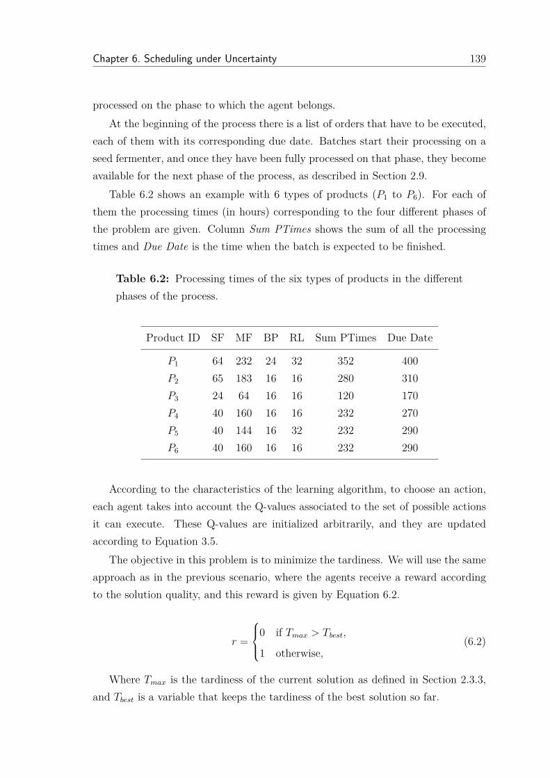
Chapter 6. Scheduling under Uncertainty 139
processed on the phase to which the agent belongs.At the beginning of the process there is a list of orders that have to be executed,
each of them with its corresponding due date. Batches start their processing on aseed fermenter, and once they have been fully processed on that phase, they becomeavailable for the next phase of the process, as described in Section 2.9.
Table 6.2 shows an example with 6 types of products (P1 to P6). For each ofthem the processing times (in hours) corresponding to the four different phases ofthe problem are given. Column Sum PTimes shows the sum of all the processingtimes and Due Date is the time when the batch is expected to be finished.
Table 6.2: Processing times of the six types of products in the differentphases of the process.
Product ID SF MF BP RL Sum PTimes Due Date
P1 64 232 24 32 352 400P2 65 183 16 16 280 310P3 24 64 16 16 120 170P4 40 160 16 16 232 270P5 40 144 16 32 232 290P6 40 160 16 16 232 290
According to the characteristics of the learning algorithm, to choose an action,each agent takes into account the Q-values associated to the set of possible actionsit can execute. These Q-values are initialized arbitrarily, and they are updatedaccording to Equation 3.5.
The objective in this problem is to minimize the tardiness. We will use the sameapproach as in the previous scenario, where the agents receive a reward accordingto the solution quality, and this reward is given by Equation 6.2.
r =
0 if Tmax > Tbest,
1 otherwise,(6.2)
Where Tmax is the tardiness of the current solution as defined in Section 2.3.3,and Tbest is a variable that keeps the tardiness of the best solution so far.

140 Chapter 6. Scheduling under Uncertainty
As there was no information about previous schedule executions, or about previ-ous breakdowns on the machines, we executed the algorithm several times in orderto visualize the solutions and estimate which resources could be considered as crit-ical. Figure 6.15 shows an example of a solution for this problem. In this case wesee 12 machines, which are grouped in the following way:
• Seed Fermentation: M1,M2
• Main Fermentation: M3, ...,M6
• Broth Preparation: M7, ...,M11
• Recovery Line: M12
It is important to remember that queues are not possible in this environment. Ifthe processing of a batch is finished and there is no resource available in the nextstage, the batch has to remain in the current resource until it can move forward.
When analyzing the problem, the attention could initially be focused on therecovery line, because only one batch can be processed at a given time, and thereis only one resource in this stage of the process. But if we analyze the solutionpresented in Figure 6.15, it is possible to see that the seed fermentation is actuallya red spot, as both fermenters are constantly working (five batches are scheduledone after the other). We can also notice that batches take longer to process in themain fermentation phase, and less during broth preparation, which somehow allowsto make the process in the recovery line more active.
From this analysis we conclude that the resources belonging to the seed fermen-tation stage are the ones that can be considered as critical. Therefore, is in this partof the schedule where slack time might be needed in order to make the schedule morerobust. In this case we incorporate the slack based approach proposed in Section6.4.
6.5.1 Experimental Results
In this section, we present the results of the computational experiments for 11 prob-lem instances involving 10, 15, 20 and 30 batches. The results are compared withthe optimal solutions (presented in [Gicquel et al. (2012)] and calculated using theCPLEX solver), and with the results reported by a Genetic Algorithm proposedin [Borodin et al. (2011)].

Chapter 6. Scheduling under Uncertainty 141
Figure6.15:Ex
ampleof
apo
ssible
solutio
nforthehy
brid
flow
shop
prob
lem.

142 Chapter 6. Scheduling under Uncertainty
Table 6.3 represents the overall comparison of the results. The CPLEX bestcolumn contains the optimal solutions, GA best - the GA results, computed in GAtime. Columns QL best and QL time show the results corresponding to the Q-Learning algorithm.
As the objective of both approaches is to minimize the tardiness, the columnsshowing the best solutions are reporting the weighted tardiness for each of the in-stances. The columns reporting the computational times show the time (in seconds)it took the algorithm to find the corresponding solution.
There are some parameters that need to be defined for the execution of thelearning algorithm. The learning rate (α) used was 0.1, the discount factor (γ) 0.8and the epsilon parameter for the action selection strategy was 0.1. The algorithmwas executed for 10000 iterations, as in the previous scenarios.
From Table 6.3 it is possible to see that the GA outperforms the QL in mostcases. It is important to notice that the solutions of the learning algorithm areclose in quality to the best found, but the computational time is always significantlylower, also we have to remember that its main goal was to provide robust schedulesthat could handle some level of uncertainty.
Table 6.3: Overall comparison table in terms of tardiness.
Instance CPLEX best GA best GA time QL best QL time
N10_1 90 93 5 98 0.7N10_2 30 30 17 37 1.5N10_3 42 44 6 54 0.9N10_4 49 50 5 59 1.3N10_5 43 45 12 58 1.5N15_1 73 76 25 84 3.3N15_2 43 45 34 56 3.6N15_3 57 66 75 75 3.4N20_1 52 54 180 61 5.4N20_2 58 64 194 75 5.4N30_1 - 186 1560 194 6.5

Chapter 6. Scheduling under Uncertainty 143
6.5.2 Conclusions about the Hybrid Flow Shop Experiments
The main conclusion is that both the GA and RL approaches are able to efficientlysolve the considered batch scheduling problem. Each approach showed its own ben-efits. According to [Borodin et al. (2011)], the GA represented a classical approachwhich was based on a Mixed Integer Linear Programming (MILP) model. Solutionsof high quality were obtained but a drawback of this classical approach is its lowrobustness - indeed, the schedule that corresponds to a high-quality solution is astight as possible and not ready to be adapted in case an unexpected event occurs.In this case, a new schedule that takes into account the occurred events must becomputed, which means that the problem will be solved from scratch.
The Reinforcement Learning approach is capable of handling this issue. Its maingoal is to quickly compute a robust schedule. For instance, in real situations it oftenhappens that a planner needs a schedule in a few seconds to report to the customerwhether the new order can be processed by this or that due-date. In this approach itis also possible to start from an initial use of the machines, i.e. non-empty resources.This is useful for example in the case when orders are not finished during the day,and a new schedule has to be constructed for the next day, but some machines stillhave work to finish.
Computational results proved that the GA is able to obtain very good solutions(comparing to the exact solutions), whereas the learning algorithm was able toobtain robust solutions close to the optimal ones, and it reported significantly lowercomputational time.
In overall, this case study demonstrated that a real-life complex hybrid flow-shopscheduling problem, which is difficult to solve by exact methods in the standardMILP formulation, can be efficiently solved by a meta-heuristic technique - on theone hand; and formulated in a lighter way to be suitable for obtaining more robustschedules faster and easier by an RL method - on the other.
6.6 Summary
In this chapter we presented the results of our approach when dealing with unex-pected events. We started by introducing a particular case, which we call knowndisruptions and then we explained the process of generating new FJSSP instancesin order to incorporate extra information to the problem, such as release dates, due

144 Chapter 6. Scheduling under Uncertainty
dates and machine breakdowns. The concept of criticality is defined and a newslack-based approach is proposed, in order to deal with uncertainty in a proactiveway. This approach uses some of the ideas behind the existing slack based tech-niques, but presents a new way to add the extra execution times to the operations.The main idea is to provide a solution that is robust enough to handle some levelof uncertainty, without loosing too much in optimality. Finally, we presentd someresults obtained from the application of a learning algorithm to the solution of ahybrid flow shop scenario, which was based on a real-world case.

Chapter 7
Conclusions
Scheduling problems are present in every situation where a given set of tasks thatrequires the allocation of resources to time slots has to be performed. Constructing aschedule is a common procedure that we usually perform in our daily life, but whenthe number of constraints that have to be met increase and the number of tasksand resources grow, then constructing a schedule that satisfies all the requirementsis not so straightforward.
Scheduling is an active research field in which several important challenges arise.For example, dealing with uncertainty is a research topic that is recently receivingmore attention. It is common to face unexpected events in scheduling environments,specially in manufacturing, which is the kind of problem this dissertation focuses on.In manufacturing environments machines can break down, orders can take longerthan expected and all these events will make the original schedule fail. That is whyit is preferable to have a solution that is robust enough to absorb some level ofuncertainty, instead of a possibly optimal one, which will fail in the presence of anysmall disruption.
In this thesis we presented a generic multi-agent reinforcement learning approachthat can easily be adapted to different scheduling settings. It is possible to increasethe robustness of the solutions being constructed and also to look at different ob-jective functions, like the tardiness or the makespan. Furthermore, the proposedapproach allows the user to set, in a transparent way, certain parameters involvedin the solution construction process, in order to define the balance between robust-ness and optimality. In the next section we give an overview of the main researchresults presented in this dissertation.
145

146 Chapter 7. Conclusions
7.1 ContributionsWe started this dissertation by presenting an overview of the scheduling theory. Aclassification of the different types of schedules that can be obtained was presented,together with several scheduling scenarios, in which the complexity (given by theconstraints of the problem) was gradually increasing. These problems are listedbelow and were all addressed in this dissertation.
• Job Shop Scheduling Problem (JSSP)
• Parallel Machines Job Shop Scheduling Problem (JSSP-PM)
• Flexible Job Shop Scheduling Problem (FJSSP)
• Stochastic Flexible Job Shop Scheduling Problem
• Online Scheduling (two phases, four machines each)
• Hybrid Flow Shop Scheduling (based on a real-world problem)
In Chapter 3, besides giving an overview of Reinforcement Learning and Multi-Agent Reinforcement Learning, we introduced the main concepts that have to betaken into account when solving a scheduling problem using Reinforcement Learning.Important definitions like changing action sets and transition dependencies wereadapted from literature and introduced using examples.
Chapter 4 started by introducing in detail what we call the ‘basic’ learning ap-proach, which is initially defined for the job shop scheduling problem and later onadapted in order to solve the other scenarios described in Chapter 2. The learn-ing method implemented was a Q-Learning algorithm, for which different feedbacksignals were studied. This QL algorithm was adapted and combined with othertechniques in order to satisfy the extra constraints of the parallel machines job shopscheduling and the flexible job shop scheduling. In the latter, an optimization tech-nique was used in order to improve the quality of the solutions. In all the cases theresults were compared with state of the art techniques reported in literature andour approach was able to obtain comparable results.
In the case of the online scheduling problem we used Learning Automata tolearn how to distribute the incoming orders of two types of products among parallelmachines. Experiments were developed using the three possible update schemes.The results of the experiments showed that the LR−P scheme was able to yieldbetter results compared to the other two reward schemes (LR−I and LR−εP ).

Chapter 7. Conclusions 147
The more common sources of uncertainty in scheduling were summarized inChapter 5. Important questions were answered, such as: what is robustness? andhow to measure how robust a schedule is?. Furthermore, different types of ap-proaches to deal with uncertainty were studied. These methods can be classified asreactive or proactive. We explained in detail some existing proactive approaches,mainly slack-based techniques, as this background was needed to understand thenew slack-based method we proposed, which was introduced later in Chapter 6. Itis also in this chapter that experiments concerning stochastic scheduling are per-formed. In order to measure the performance of the approach under uncertainty,several problem instances were generated. The process of generating the instanceswas thoroughly explained such that these could be used as a benchmark for furtherresearch.
The new slack-based method proposed in this chapter bases its behavior onsomething we defined as the criticality of the machines. This concept is used inorder to define the parts of the schedule that are more likely to need extra executiontime. Experiments in this regard are also reported, in which the main idea wasto obtain solutions with a good balance between optimality and robustness. Thisapproach was applied when solving the hybrid flow shop scheduling scenario, whichis based on a real-world application. An important added value of our approachis the fact that it allows the user to set some parameters involved in the solutionconstruction process, for example, the desired level of robustness, in a very intuitiveway. The contributions are graphically summarized in Figure 7.1.
In general, we receive a scheduling problem, and additionally there can be a setof user specifications. These user specifications can be preferences, extra constraintsto the problem, or preferred values for specific parameters. All this information isgiven to our MARL approach, which depending on the characteristics of the problemand the user specifications, will solve it on its own, or in combination with the modeoptimization procedure and/or the slack-based approach. This will provide as outputa near-optimal schedule, which can have different levels of robustness. It is alsopossible to identify which are the critical machines and provide a visualization of theresulting schedule in the form of a gantt chart. This visualization helps the user tocarefully analyze the proposed solution, and maybe change some parameter settingsin order to analyze what will happen if the system is under different circunstances,or just to get a better balance between robustness and optimality.

148 Chapter 7. Conclusions
Figure 7.1: Graphical representation of the contributions of this disser-tation.
7.2 Future WorkIn this section we list some ideas to extend the research presented in this dissertation.
• Integrated Approach: In Chapter 4 we proposed a hierarchical approachfor the Flexible Job Shop Scheduling Problem, which was also used to solvethe stochastic version of this problem. As explained before, hierarchical ap-proaches divide the problem in two steps: routing and sequencing, followingthe classical ‘assign-then-sequence’ rule, which means that a machine is as-signed to each operation and once this machine-operation assignment has beendone, the operations are sequenced on the assigned resources. It will be inter-esting to explore an integrated approach, which takes care of the routing andthe sequencing at the same time.
• Multiple objectives: When solving the stochastic flexible job shop schedul-ing in Chapter 6, new instances were generated in order to measure the perfor-mance of the algorithm under unexpected events. These instances had releaseand due dates incorporated, which made it possible to report results either interms of makespan or in terms of tardiness. The possibility of dealing with

Chapter 7. Conclusions 149
multiple objectives at the same time would also be an interesting avenue forfuture research. This would mean that the feedback signals and the objectivefunctions of the current approach should be re-defined.
• LA for unexpected events: In Chapter 4 we proposed a solution to anonline scheduling problem using LA. In this case the information about howmany jobs have to be processed and their corresponding processing times is notknown in advance. The experiments performed in this scenario showed thatLA can cope with unknown joblengths, unknown future jobs and unknownmachine speeds, without needing heuristics or additional information. Wecould take advantage of this and incorporate LA in the slack-based approachproposed in this dissertation. This will allow to learn about the criticality ofthe machines and improve the way the robust solutions are constructed for aspecific type of problem.
• Highly constrained hybrid flow shop scheduling problem: In thescheduling community it is common to work with benchmarks, which notalways represent all aspects of real life scheduling problems. It is well knownthat industries need systems for optimized production scheduling that adjustexactly to the conditions in the production plant. One case of such a prob-lem is the highly constrained hybrid flow shop scheduling scenario describedin [Urlings (2010)]. This problem involves some extra constraints that were notpresent in the scheduling scenarios addressed in this dissertation. The appli-cation of our approach to such a complex environment is currently under study.
• Cuban real-world application: In the cuban context, more specifically incompanies responsible for the production of spare pieces for industrial ma-chines, there is a lack of effective methods that can contribute to the schedul-ing of the production process. The repair shop ‘Manual Fajardo’, located inGranma, a province at the east of Cuba, is responsible for the manufacturing(and repairing) of several pieces of equipments that are used by the differentmachines involved in the sugar production process. The production chain isstructured in a way that all the tasks have to follow the same production path,which means that they are executed by the machines in the same order. This

150 Chapter 7. Conclusions
fits the definition of flow shop scheduling.
The repair shop is experiencing delays, mainly due to the arrival of extra orderswhich sometimes have high priorities due to the kind of pieces being requested.This kind of requests are more common in the sugar harvesting season.
This is a potential real-world application that could benefit from the researchpresented in this dissertation.

Curriculum Vitae
Education
• Bachelor in Computer Science, Universidad Central ‘Marta Abreu’ de LasVillas (UCLV), Cuba, 2004.
• Master in Computer Sciences, Universidad Central ‘Marta Abreu’ de Las Villas(UCLV), Cuba, 2007.
• Master of Computer Sciences, Vrije Universiteit Brussel (VUB), Belgium,2008.
Publications
Journals, Book Chapters and Lecture Notes
• Martínez Y., Nowé A., Suárez J., Bello R. (2011) A Reinforcement Learn-ing Approach for the Flexible Job Shop Scheduling Problem. Lecture Notesin Computer Science. Proceedings of the fifth International Conference onLearning and Intelligent Optimization(LION5); Vol.6683:pp.253-262.
• Martínez Y., Van Vreckem B., Catteeuw D., Nowé A. (2010) Application ofLearning Automata for Stochastic Online Scheduling. Recent Advances in Op-timization and its Applications in Engineering. Springer Berlin Heidelberg;Eds. Diehl M., Glineur F., Jarlebring E., Michiels W.; pp.491-498.
• Puris A., Bello R., Martínez Y., Trujillo Y., Nowé A. (2008) Two-stage ACOto solve the job shop scheduling problem. Lecture Notes in Computer Science.Book ‘Progress in Pattern Recognition, Image Analysis and Applications’;Vol.4756:pp.447-456.
151

152 Curriculum Vitae
• Rodríguez L., Casas G., Grau R., Martínez Y. (2008) Fuzzy Scan Method toDetect Clusters. International Journal of Biological and Life Sciences; Vol.3:pp.111-115.
• Puris A., Bello R., Martínez Y., Nowé A. (2007) Two-stage ant colony opti-mization for solving the traveling salesman problem. Lecture Notes in Com-puter Sciences. Book ‘Nature Inspired Problem-Solving Methods in KnowledgeEngineering’. Vol.4528(1):pp.307-316.
• Puris A., Bello R., Nowé A., Martínez Y. (2006) Two-Stage Ant Colony Systemfor Solving the Traveling Salesman Problem. Journal Research in ComputingScience.Vol.26(1):pp.85-92.
Conference Proceedings• Martínez Y., Nowé A., Suárez J., Bello R. (2011) Solution to the Flexible Job
Shop Scheduling Problem using Reinforcement Learning. In: Proceedings ofthe 14th International Convention and Fair Informatica 2011. Havana, Cuba.
• Kaddoum E., Martínez Y., Wauters T., (2010) Adaptive methods for flexiblejob shop scheduling with due-dates , release-dates and machine perturbations.In: Workshop on Self-tuning, self-configuring and self-generating search heuris-tics (Self* 2010). Krakow, Poland; 2010.
• Martínez Y., Wauters T., Nowé A., Verbeeck, K., De Causmaecker P., Bello,P. (2010) Reinforcement Learning Approaches for the Parallel Machines JobShop Scheduling Problem. In: Proceedings of the Cuba-Flanders Workshop onMachine Learning and Knowledge Discovery. Santa Clara, Cuba.
• De Causmaecker P., Verbeeck K., Wauters T., Martínez Y. (2010) Scalabledecentralised approaches for job shop scheduling. In: Proceedings of the 24thEuropean Conference on Operational Research EURO XXIV. Lisbon, Portu-gal.
• Wauters T., Martínez Y., De Causmaecker P., Nowé A., Verbeeck K. (2010)Reinforcement Learning approaches for the Parallel Machines Job Shop Schedul-ing Problem. In: Proceedings of ITEC2010 - International conference on inter-disciplinary research on technology, education and communication. Kortrijk,Belgium.

Curriculum Vitae 153
• Martínez Y., Van Vreckem B., Catteeuw D., Nowé A. (2009) Multi-StageScheduling Problem with Parallel Machines. In: Proceedings of BFG’09, the14th Belgian-French-German Conference on Optimization. Leuven, Belgium.
• Martínez Y., Nowé A. (2009) A Multi-Agent learning approach for the JobShop Scheduling Problem. In: Proceedings of the 23rd European Conferenceon Operational Research. Bonn, Germany.
• Puris A., Bello R., Nowé A., Martínez Y. (2006) Improving Ant Colony Op-timization to solve the Travelling Salesman Problem. In: Proceedings of 18thBenelux Conference on Artificial Intelligence (BNAIC 2006).
Participation in Conferences and Summer Schools
• European Workshop on Reinforcement Learning. September 9-11, Athens,Greece, 2011.
• ACAI Summer School on Automated Planning and Scheduling, ACAI’11.Freiburg, Germany, June 7-10, 2011.
• Symposium ‘OR problems and AI techniques’, March 2011, KULAK, Kortrijk.
• Learning and Intelligent OptimizatioN, LION 5, January 17-21, 2011, Rome,Italy.
• 11th International Conference on Parallel Problem Solving from Nature (PPSN).Workshop on Self-tuning, self-configuring and self-generating search heuristics(Self* 2010), Krakow, Poland, September 11-15, 2010.
• Cuba-Flanders Workshop on Machine Learning and Knowledge Discovery,Santa Clara, Cuba, February 5-8, 2010.
• Summer School: Advanced Course in Artificial Intelligence, ACAI’09, Belfast,August 23-29, 2009.
• 14th Belgian-French-German Conference on Optimization, Leuven, September14-18, 2009.
• 23rd European Conference on Operational Research, Bonn, Germany, July5-8, 2009.

154 Curriculum Vitae
• Eight International Conference on Autonomous Agents and Multiagent Sys-tems, Budapest, Hungary, May 10-15, 2009.
• Doctor Honoris Causa, Louvain-La-Neuve, Belgium, 2008.
• TAAME 07 - Theory And Applications of MEtaheuristics - Tutorial Day, KaHoSint Lieven, Gent, Belgium, 2007.
• Biologically inspired robotics: From evolving to self replicating and self repair-ing machines, Iridia - ULB, Belgium, 2007.

Bibliography
[Aloulou & Portmann (2005)] Aloulou, M. A. & Portmann, M.-C. (2005).An efficient proactive-reactive scheduling approach to hedge against shopfloor disturbances. In: Multidisciplinary scheduling: theory and applications(Kendall, G., Burke, E. K., Petrovic, S. & Gendreau, M., eds.).Springer US, pp. 223–246. Cited on pages 108 and 109.
[Auer et al. (2002)] Auer, P., Cesa-Bianchi, N. & Fischer, P. (2002). Finite-time analysis of the multiarmed bandit problem. Machine learning 47, 235–256.Cited on page 54.
[Baker (1974)] Baker, K. (1974). Introduction to sequencing and scheduling. JohnWiley & Sons. Cited on page 24.
[Beasley (1990)] Beasley, J. E. (1990). OR-Library. URL http://people.
brunel.ac.uk/~mastjjb/jeb/info.html. Cited on pages 26 and 74.
[Beck & Wilson (2007)] Beck, J. & Wilson, N. (2007). Proactive algorithms forjob shop scheduling with probabilistic durations. Journal of Artificial Intelli-gence Research 28(1), 183–232. Cited on page 108.
[Bellman (1957)] Bellman, R. (1957). Dynamic Programming. Princenton, NJ,USA: Princeton University Press. Cited on pages 48 and 49.
[Ben-Tal & Nemirovski (2000)] Ben-Tal, A. & Nemirovski, A. (2000). Robustsolutions of Linear Programming problems contaminated with uncertain data.Mathematical Programming 88, 411–424. Cited on pages 103 and 106.
[Bernstein et al. (2002)] Bernstein, D., Givan, R., Immerman, N. & Zilber-stein, S. (2002). The complexity of decentralized control of Markov deci-sion processes. Mathematics of Operations Research 27(4), 819–840. Cited onpages 57 and 58.
155

156 BIBLIOGRAPHY
[Bertsekas (1995)] Bertsekas, D. (1995). Dynamic Programming and OptimalControl (Volume 1). Athena Scientific, third ed. Cited on page 48.
[Bertsimas & Sim (2004)] Bertsimas, D. & Sim, M. (2004). The price of robust-ness. Operations research 52(1), 1–34. Cited on page 106.
[Billaut et al. (2008)] Billaut, J., Moukrim, A. & Sanlaville, E. (2008).Flexibility and robustness in scheduling. Wiley. Cited on pages 3, 106, and 107.
[Borodin et al. (2011)] Borodin, D., Van Vreckem, B. & De Bruyn, W.(2011). Case study: an effective genetic algorithm for the chemical batch pro-duction scheduling. In: Proceedings of the 5th Multidisciplinary InternationalScheduling Conference: Theory & Applications (MISTA 2011). Phoenix, Ari-zona. Cited on pages 34, 140, and 143.
[Brandimarte (1993)] Brandimarte, P. (1993). Routing and scheduling in a flex-ible job shop by tabu search. Annals of Operations Research 41(3), 157–183.Cited on pages 90, 91, and 119.
[Brucker (2007)] Brucker, P. (2007). Scheduling Algorithms. Springer. Cited onpage 12.
[Bush & Mosteller (1955)] Bush, F. & Mosteller, R. R. (1955). StochasticModels for Learning. Wiley. Cited on page 51.
[Cassandra (1998)] Cassandra, A. R. (1998). Exact and Approximate Algorithmsfor Partially Observable Markov Decision Processes. Phd thesis, Brown Uni-versity. Cited on page 47.
[Castillo & Roberts (2001)] Castillo, I. & Roberts, C. (2001). Real-time con-trol/scheduling for multi-purpose batch plants. Computers & industrial engi-neering 41(2), 211–225. Cited on pages 33 and 100.
[Charnprasitphon (2007)] Charnprasitphon, A. (2007). Modeling and analysisof the batch production scheduling problem for perishable products with setuptimes. Phd thesis, Georgia Institute of Technology. Cited on page 13.
[Chiang & Fox (1990)] Chiang, W. & Fox, M. (1990). Protection against uncer-tainty in a deterministic schedule. In: Proceedings 4th International Conference

BIBLIOGRAPHY 157
on Expert Systems and the Leading Edge in Production and Operations Man-agement. Cited on page 111.
[Church & Uzsoy (1992)] Church, L. K. & Uzsoy, R. (1992). Analysis ofperiodic and event-driven rescheduling policies in dynamic shops. Interna-tional Journal of Computer Integrated Manufacturing 5(3), 153–163. Cited onpage 109.
[Cohn (2007)] Cohn, A. (2007). Robust Schdule Planning and Recovery: The Roleof Operations Research. Cited on page 105.
[Conway et al. (1967)] Conway, R., Maxwell, W. & Miller, L. W. (1967).Theory of scheduling. Addison-Wesley. Cited on pages 20 and 21.
[Davenport & Beck (2000)] Davenport, A. & Beck, J. (2000). A survey of tech-niques for scheduling with uncertainty. Unpublished manuscript. , 49. Cited onpages 108 and 117.
[Davenport et al. (2001)] Davenport, A., Gefflot, C. & Beck, J. C. (2001).Slack-based Techniques for Robust Schedules. In: Proceedings of the SixthEuropean Conference on Planning (ECP-2001). Cited on pages 4, 105, 111,113, and 115.
[Gabel (2009)] Gabel, T. (2009). Multi-Agent Reinforcement Learning Approachesfor Distributed Job-Shop Scheduling Problems. Ph.D. thesis, Universität Os-nabrück. Cited on pages 5, 38, 61, 63, 67, and 69.
[Gabel & Riedmiller (2007)] Gabel, T. & Riedmiller, M. (2007). On a Suc-cessful Application of Multi-Agent Reinforcement Learning to Operations Re-search Benchmarks. In: IEEE International Symposium on Approximate Dy-namic Programming and Reinforcement Learning. Honolulu , USA. Cited onpages 38, 70, 71, and 78.
[Gabel & Riedmiller (2008)] Gabel, T. & Riedmiller, M. (2008). Reinforce-ment learning for DEC-MDPs with changing action sets and partially ordereddependencies. In: Proceedings of the 7th International Conference on Au-tonomous Agents and Multiagent Systems (AAMAS 2008). Estoril, Portugal.Cited on page 59.

158 BIBLIOGRAPHY
[Gao (1996)] Gao, H. (1996). Building Robust schedules using temporal protection-an empirical study of constraint based scheduling under machine failure uncer-tainty. Master thesis, University of Toronto. Cited on pages 104, 105, 107, 111,and 112.
[Garey & Johnson (1979)] Garey, M. R. & Johnson, D. S. (1979). Computersand Intractability: A Guide to the Theory of NP-Completeness (Series of Booksin the Mathematical Sciences). W. H. Freeman. Cited on page 24.
[Garey et al. (1976)] Garey, M. R., Johnson, D. S. & Sethi, R. (1976). TheComplexity of Flowshop and Jobshop Scheduling. Mathematics of OperationsResearch 1(2), 117–129. Cited on pages 12, 26, and 62.
[Garrido et al. (2000)] Garrido, A., Salido, M., Barber, F. & López, M.(2000). Heuristic methods for solving job-shop scheduling problems. In: ECAI-2000 Workshop on New Results in Planning, Scheduling and Design (PuK2000).Cited on page 26.
[Gicquel et al. (2012)] Gicquel, C., Hege, L., Minoux, M. & van Canneyt,W. (2012). A discrete time exact solution approach for a complex hybridflow-shop scheduling problem with limited-wait constraints. Computers & Op-erations Research 39(3), 629–636. Cited on pages 34, 35, and 140.
[Goldsmith et al. (1996)] Goldsmith, J., Lusena, C. & Mundhenk, M. (1996).The complexity of deterministically observable finite-horizon Markov decisionprocesses. Tech. rep., University of Kentucky. Cited on page 46.
[Gomes (2000)] Gomes, C. P. (2000). Artificial intelligence and operations re-search: challenges and opportunities in planning and scheduling. The Knowl-edge Engineering Review 15(1), 1–10. Cited on pages 3, 4, and 107.
[Graham et al. (1979)] Graham, R., Lawler, E., Lenstra, J. & RinnooyKan, A. H. G. (1979). Optimization and approximation in deterministicsequencing and scheduling: a survey. Annals of Discrete Mathematics 5, 287–326. Cited on pages 3 and 17.
[Grossmann (2005)] Grossmann, I. (2005). Enterprise-wide optimization: A newfrontier in process systems engineering. AIChE Journal 51(7), 1846–1857. Citedon page 12.

BIBLIOGRAPHY 159
[Hartmann (1999)] Hartmann, S. (1999). Project Scheduling Under Limited Re-sources: Models, Methods, and Applications. Springer. Cited on page 121.
[Hasan et al. (2007)] Hasan, S., Sarker, R. & Cornforth, D. (2007). Hybridgenetic algorithm for solving job-shop scheduling problem. In: 6th IEEE/ACISInternational Conference on Computer and Information Science (ICIS 2007).Cited on page 77.
[Herrmann et al. (1993)] Herrmann, J., Lee, C. & Snowdon, J. (1993). A clas-sification of static scheduling problems. Complexity in Numerical Optimization, 203–253. Cited on page 17.
[Herroelen & Leus (2005)] Herroelen, W. & Leus, R. (2005). Project schedul-ing under uncertainty: Survey and research potentials. European Journal ofOperational Research 165(2), 289–306. Cited on pages 3 and 107.
[Ho et al. (2007)] Ho, N., Tay, J. & Lai, E. (2007). An effective architecture forlearning and evolving flexible job-shop schedules. European Journal of Opera-tional Research 179(2), 316–333. Cited on page 91.
[Jennings et al. (1998)] Jennings, N. R., Sycara, K. & Wooldridge, M.(1998). A roadmap of agent research and development. Autonomous Agentsand Multi-agent Systems 1, 7–38. Cited on pages 42 and 54.
[Jensen (2001)] Jensen, M. T. (2001). Improving robustness and flexibility oftardiness and total flow-time job shops using robustness measures. Applied SoftComputing 1(1), 35–52. Cited on page 109.
[Kaddoum (2011)] Kaddoum, E. (2011). Optimization under Constraints of Dis-tributed Complex Problems using Cooperative Self-Organization. Phd thesis,Université Paul Sabatier - Toulouse III. Cited on pages 109, 121, and 123.
[Kaddoum et al. (2010)] Kaddoum, E., Martinez, Y., Wauters, T., Ver-beeck, K., Nowe, A., De Causmaecker, P., Vanden Berghe, G.,Gleizes, M.-P. & George, J.-P. (2010). Adaptive methods for flexible jobshop scheduling with due-dates , release-dates and machine perturbations. In:Workshop on Self-tuning, self-configuring and self-generating search heuristics(Self* 2010). Krakow, Poland. Cited on page 8.

160 BIBLIOGRAPHY
[Kaelbling et al. (1996)] Kaelbling, L., Littman, M. & Moore, A. (1996).Reinforcement learning: A survey. Journal of artificial intelligence research 4,237–285. Cited on pages 43 and 45.
[Kaminka (2004)] Kaminka, G. A. (2004). Multi-Agent Systems. Cited onpage 54.
[Lambrechts et al. (2010)] Lambrechts, O., Demeulemeester, E. & Herroe-len, W. (2010). Time slack-based techniques for robust project scheduling sub-ject to resource uncertainty. Annals of Operations Research 186(1), 443–464.Cited on page 109.
[Le Pape (1991)] Le Pape, C. (1991). Constraint propagation in planning andscheduling. Tech. rep., Standford University. Cited on page 105.
[Leon et al. (1994)] Leon, V. J., Wu, S. D. & Storer, R. H. (1994). Robust-ness measures and robust scheduling for job shops. IIE transactions 26(5),32–43. Cited on pages 106 and 109.
[Lining & Chen (2010)] Lining, X. & Chen, Y. (2010). A Knowledge-Based AntColony Optimization for Flexible Job Shop Scheduling Problems. Applied SoftComputing 10(3), 888–896. Cited on page 91.
[Littman (1994)] Littman, M. (1994). Markov games as a framework for multi-agent reinforcement learning. In: Proceedings of the Eleventh InternationalConference on Machine Learning. San Francisco, CA: Morgan Kaufmann. Citedon page 56.
[Littman et al. (1995)] Littman, M., Cassandra, A. & Kaelbling, L. (1995).Learning policies for partially observable environments : Scaling up. In: Read-ing in Agents (Huhns, M. N. & Singh, M. P., eds.). Morgan KaufmannPublishers Inc., pp. 495 – 503. Cited on page 47.
[Lui Cheng (2008)] Lui Cheng, L. (2008). Robust scheduling in forest operationsplanning. Master thesis, Massachusetts Institute of Technology. Cited onpage 106.
[Martínez et al. (2011)] Martínez, Y., Nowé, A., Suárez, J. & Bello, R.(2011). A Reinforcement Learning Approach for the Flexible Job Shop Schedul-

BIBLIOGRAPHY 161
ing Problem. Lecture Notes in Computer Science. Proceedings of the fifth In-ternational Conference on Learning and Intelligent Optimization(LION5).Vol.6683, pp. 253–262. Cited on page 90.
[Martínez et al. (2010)a] Martínez, Y., Vreckem, B., Catteeuw, D. &Nowé, A. (2010a). Application of Learning Automata for Stochastic On-line Scheduling. In: Recent Advances in Optimization and its Applications inEngineering (Diehl, M., Glineur, F., Jarlebring, E. & Michiels, W.,eds.). Springer, pp. 491–498. Cited on pages 93 and 94.
[Martínez et al. (2010)b] Martínez, Y., Wauters, T., De Causmaecker, P.,Nowe, A., Verbeeck, K., Bello, R. & Suarez, J. (2010b). Reinforce-ment Learning Approaches for the Parallel Machines Job Shop Scheduling Prob-lem. In: Proceedings of the Cuba-Flanders Workshop on Machine Learning andKnowledge Discovery. Santa Clara, Cuba. Cited on page 81.
[Martínez Jiménez (2008)] Martínez Jiménez, Y. (2008). A Multi-Agent Learn-ing Approach for the Job Shop Scheduling Problem. Master thesis, Vrije Uni-versiteit Brussel. Cited on page 75.
[Megow et al. (2006)] Megow, N., Uetz, M. & Vredeveld, T. (2006). Modelsand Algorithms for Stochastic Online Scheduling. Mathematics of OperationsResearch 31(3), 513–525. Cited on page 93.
[Méndez et al. (2006)] Méndez, C., Cerdá, J., Grossmann, I., Harjunkoski,I. & Fahl, M. (2006). State-of-the-art review of optimization methods forshort-term scheduling of batch processes. Computers & chemical engineering30(6-7), 913–946. Cited on page 14.
[Metaxiotis et al. (2005)] Metaxiotis, K., Askounis, D. & Psarras, J. (2005).Expert systems technology in production planning and scheduling. In: Intel-ligent Knowledge-Based Systems (Leondes, C. T., ed.), vol. 3. Springer US,pp. 55–75. Cited on page 12.
[Moriarty et al. (1999)] Moriarty, D. E., Schultz, A. C. & Grefenstette,J. J. (1999). Evolutionary Algorithms for Reinforcement Learning. Journal ofArtificial Intelligence Research 11, 241–276. Cited on pages 43 and 45.

162 BIBLIOGRAPHY
[Narendra & Thathachar (1974)] Narendra, K. S. & Thathachar, M. A. L.(1974). Learning automata - A survey. IEEE Transactions on Systems, Man,and Cybernetics, , 323–334. Cited on page 51.
[Nhu Binh HO (2005)] Nhu Binh HO, J. C. T. (2005). Evolving DispatchingRules for solving the Flexible Job-Shop Problem. The 2005 IEEE Congress onEvolutionary Computation. 3, 2848–2855. Cited on page 37.
[Nowé et al. (2012)] Nowé, A., Vrancx, P. & De Hauwere, Y.-M. (2012).Game Theory and Multi-agent Reinforcement Learning. In: ReinforcementLearning: State-of-the-Art (Wiering, M. & Van Otterlo, M., eds.).Springer, pp. 441–470. Cited on page 56.
[Peeters (2008)] Peeters, M. (2008). Solving Multi-Agent Sequential DecisionProblems Using Learning Automata. Phd thesis, Vrije Universiteit Brussel.Cited on pages 33 and 94.
[Pezzella et al. (2008)] Pezzella, F., Morganti, G. & Ciaschetti, G. (2008).A genetic algorithm for the flexible job-shop scheduling problem. Computers &Operations Research 35(10), 3202–3212. Cited on pages 91 and 120.
[Pinedo (2008)] Pinedo, M. (2008). Scheduling: theory, algorithms, and systems,Third Edition. Springer Verlag. Cited on pages 2, 11, 13, 20, and 33.
[Policella (2005)] Policella, N. (2005). Scheduling with Uncertainty A ProactiveApproach using Partial Order Schedules. Phd thesis, Università degli Studi diRoma "La Sapienza". Cited on page 104.
[Puris et al. (2007)] Puris, A., Bello, R., Trujillo, Y., Nowe, A. & Mar-tinez, Y. (2007). Two-stage ACO to solve the job shop scheduling problem.Lecture Notes in Computer Science. Book "Progress in Pattern Recognition,Image Analysys and Applications" 4756, 447–456. Cited on page 77.
[Puterman (1994)] Puterman, M. L. (1994). Markov Decision Processes: DiscreteStochastic Dynamic Programming. New York, NY, USA: John Wiley & Sons,Inc. Cited on pages 45 and 49.
[Rodrigues Gomes & Kowalczyk (2009)] Rodrigues Gomes, E. & Kowalczyk,R. (2009). Dynamic Analysis of Multiagent Q-learning with Exploration e-

BIBLIOGRAPHY 163
greedy. In: Proceedings of the 26th International Conference on Machine Learn-ing. Cited on page 69.
[Rossi & Boschi (2009)] Rossi, A. & Boschi, E. (2009). A hybrid heuristic tosolve the parallel machines job-shop scheduling problem. Advances in Engi-neering Software 40(2), 118–127. Cited on pages 28, 80, and 81.
[Ruiz et al. (2008)] Ruiz, R., Şerifoğlu, F. S. & Urlings, T. (2008). Modelingrealistic hybrid flexible flowshop scheduling problems. Computers & OperationsResearch 35(4), 1151–1175. Cited on page 14.
[Russell & Norvig (2003)] Russell, S. & Norvig, P. (2003). Artificial Intelli-gence: A Modern Approach (2nd Edition). Prentice Hall. Cited on page 41.
[Sabuncuoglu & Goren (2009)] Sabuncuoglu, I. & Goren, S. (2009). Hedgingproduction schedules against uncertainty in manufacturing environment with areview of robustness and stability research. International Journal of ComputerIntegrated Manufacturing 22(2), 138–157. Cited on pages 106 and 109.
[Shapley (1953)] Shapley, L. S. (1953). Stochastic Games. Proceedings of theNational Academy of Sciences of 39, 1095–1100. Cited on page 56.
[Shen (2002)] Shen, W. (2002). Distributed Manufacturing Scheduling Using In-telligent Agents. IEEE Intelligent Systems 17, 88–94. Cited on page 12.
[Simon & Lea (1973)] Simon, H. & Lea, G. (1973). Problem solving and ruleinduction: A unified view. Knowledge and Cognition , 105 – 128. Cited onpage 41.
[Soyster (1973)] Soyster, A. L. (1973). Convex programming with set-inclusiveconstraints and applications to inexact linear programming. Operations Re-search 21(5), 1154–1157. Cited on page 106.
[Sutton & Barto (1998)] Sutton, R. S. & Barto, A. G. (1998). ReinforcementLearning: An Introduction. The MIT Press. Cited on pages 5, 43, 48, 50, 52,and 53.
[Sycara (1998)] Sycara, K. P. (1998). Multiagent Systems. AI Magazine , 79–92.Cited on pages 54 and 55.

164 BIBLIOGRAPHY
[Tsetlin (1962)] Tsetlin, M. (1962). On the behavior of finite automata in randommedia. Automation and Remote Control 22, 1210–1219. Cited on page 51.
[Tsitsiklis (1994)] Tsitsiklis, J. (1994). Asynchronous stochastic approximationand Q-learning. Machine Learning 16, 185–202. Cited on page 50.
[Urlings (2010)] Urlings, T. (2010). Heuristics and metaheuristics for heavilyconstrained hybrid flowshop problems. Phd thesis, Universidad Politécnica deValencia. Cited on pages 6 and 149.
[Van Peteghem & Vanhoucke (2008)] Van Peteghem, V. & Vanhoucke, M.(2008). A Genetic Algorithm for the Multi-Mode Resource-Constrained ProjectScheduling Problem. Tech. Rep. January, Ghent University. Cited on pages 85,87, and 120.
[Ventresca & Ombuki (2004)] Ventresca, M. & Ombuki, B. (2004). Ant colonyoptimization for job shop scheduling problem. In: Proceeding of 8th IASTEDInternational Conference On Artificial Intelligence and Soft Computing (ASC2004), February. Cited on page 78.
[Vieira et al. (2003)] Vieira, G. E., Herrmann, J. W. & Lin, E. (2003).Rescheduling Manufacturing Systems: A Framework of Strategies, Policies,and Methods. Journal of Scheduling 6(1), 39–62. Cited on page 109.
[Wang & Shen (2007)] Wang, L. & Shen, W. (eds.) (2007). Process Planningand Scheduling for Distributed Manufacturing. Springer. Cited on page 2.
[Wauters et al. (2010)] Wauters, T., Martinez, Y., De Causmaecker, P.,Nowe, A. & Verbeeck, K. (2010). Reinforcement Learning approachesfor the Parallel Machines Job Shop Scheduling Problem. In: Proceedings ofITEC2010 - International conference on interdisciplinary research on technol-ogy, education and communication. Kortrijk, Belgium. Cited on pages 81, 83,and 109.
[Winston (2003)] Winston, W. L. (2003). Operations Research: Applications andAlgorithms. Duxbury Pr, 4th ed. Cited on page 120.
[Wooldridge (1999)] Wooldridge, M. (1999). Intelligent Agents. In: MultiagentSystems (Weiss, G., ed.). The MIT Press, p. 51. Cited on page 42.

BIBLIOGRAPHY 165
[Wooldridge & Jennings (1995)] Wooldridge, M. & Jennings, N. (1995). Intel-ligent agents: theory and practice. The Knowledge Engineering Review 10(2),115–152. Cited on page 42.
[Wu et al. (1999)] Wu, S. D., Byeon, E.-S. & Storer, R. H. (1999). A Graph-Theoretic Decomposition of the Job Shop Scheduling Problem to AchieveScheduling Robustness. Operations Research 47(1), 113–124. Cited onpage 109.
[Wu et al. (2005)] Wu, T., Ye, N. & Zhang, D. (2005). Comparison of dis-tributed methods for resource allocation. International Journal of ProductionResearch 43(3), 515–536. Cited on pages 63 and 67.
[Zhang (1996)] Zhang, W. (1996). Reinforcement Learning for Job Shop Schedul-ing. Ph.D. thesis, Oregon State University. Cited on pages 25, 37, 38, and 44.
[Zhang & Dietterich (1995)] Zhang, W. & Dietterich, T. G. (1995). A rein-forcement learning approach to job-shop scheduling. In: Proceedings of theFourteenth International Joint Conference on Artificial Intelligence. MorganKaufmann. Cited on page 38.


Index
AAction Selection . . . . . . . . . . . . . . . . . . . . . . . . . . . . . . . . . . . . . . . . . . . . . . . . . . . . . . . . . . . . . . . 52Agents . . . . . . . . . . . . . . . . . . . . . . . . . . . . . . . . . . . . . . . . . . . . . . . . . . . . . . . . . . . . . . . . . . . . . . . . 41Artificial Intelligence (AI) . . . . . . . . . . . . . . . . . . . . . . . . . . . . . . . . . . . . . . . . . . . . . . . 3, 12, 37
BBatch Production . . . . . . . . . . . . . . . . . . . . . . . . . . . . . . . . . . . . . . . . . . . . . . . . . . . . . . . . . . . . . 13Bellman equation . . . . . . . . . . . . . . . . . . . . . . . . . . . . . . . . . . . . . . . . . . . . . . . . . . . . . . . . . . . . . .48Branch and Bound (BB) . . . . . . . . . . . . . . . . . . . . . . . . . . . . . . . . . . . . . . . . . . . . . . . . . . . 14, 37
DDecentralized Markov Decision Process (DEC-MDP) . . . . . . . . . . . . . . . . . . . . . . . . . . 58Decentralized MDP with Changing Action Sets (DEC-MDP-CAS) . . . . . . . . . . . . . 59Dynamic Programming (DP) . . . . . . . . . . . . . . . . . . . . . . . . . . . . . . . . . . . . . . . . . . . . . . 37, 48
FFlexible Job Shop Instances . . . . . . . . . . . . . . . . . . . . . . . . . . . . . . . . . . . . . . . . . . . . . . . . . . . 30Flexible Job Shop Scheduling Problem (FJSSP) . . . . . . . . . . . . . . . . . . . . . . . . 6, 30, 146Focused Time Window Slack (FTWS) . . . . . . . . . . . . . . . . . . . . . . . . . . . . . . . . . . . . . . . . 115
GGantt Chart . . . . . . . . . . . . . . . . . . . . . . . . . . . . . . . . . . . . . . . . . . . . . . . . . . . . . . . . . . . . . . . . . . .27Genetic Algorithms (GA) . . . . . . . . . . . . . . . . . . . . . . . . . . . . . . . . . . . . . . . . . . . . . . . . . . . . . .37
HHeuristic . . . . . . . . . . . . . . . . . . . . . . . . . . . . . . . . . . . . . . . . . . . . . . . . . . . . . . . . . . . . . . . . . . . . . . 31Hierarchical Approaches . . . . . . . . . . . . . . . . . . . . . . . . . . . . . . . . . . . . . . . . . . . . . . . . . . . . . . . 31Hybrid Flow Shop Scheduling . . . . . . . . . . . . . . . . . . . . . . . . . . . . . . . . . . . . . . . . . . . . .34, 146
167

168 INDEX
IIntegrated Approaches . . . . . . . . . . . . . . . . . . . . . . . . . . . . . . . . . . . . . . . . . . . . . . . . . . . . . . . . .31
JJob Shop Instances . . . . . . . . . . . . . . . . . . . . . . . . . . . . . . . . . . . . . . . . . . . . . . . . . . . . . . . . . . . . 26Job Shop Scheduling Problem (JSSP) . . . . . . . . . . . . . . . . . . . . . . . . . . . . . . . . . . 6, 24, 146
LLearning Automata (LA) . . . . . . . . . . . . . . . . . . . . . . . . . . . . . . . . . . . . . . . . . . . . . . . . . . . . . . 51Linear Programming (LP) . . . . . . . . . . . . . . . . . . . . . . . . . . . . . . . . . . . . . . . . . . . . . . . . . . . . . 37
MMarkov Decision Process (MDPs) . . . . . . . . . . . . . . . . . . . . . . . . . . . . . . . . . . . . . . . . . . . . . 46Markov Game (MG) . . . . . . . . . . . . . . . . . . . . . . . . . . . . . . . . . . . . . . . . . . . . . . . . . . . . . . . . . . .56Mixed Integer Linear Programming (MILP) . . . . . . . . . . . . . . . . . . . . . . . . . . . . . . .14, 143Multi-Agent Markov Decision Process (MMDP) . . . . . . . . . . . . . . . . . . . . . . . . . . . . . . . 57Multi-Agent Reinforcement Learning (MARL) . . . . . . . . . . . . . . . . . . . . . . . . . . . . . . . . . 56Multi-Agent Systems (MAS) . . . . . . . . . . . . . . . . . . . . . . . . . . . . . . . . . . . . . . . . . . . . . . . . . . 54
NNon-delay schedules . . . . . . . . . . . . . . . . . . . . . . . . . . . . . . . . . . . . . . . . . . . . . . . . . . . . . . . . . . 105NP-hard . . . . . . . . . . . . . . . . . . . . . . . . . . . . . . . . . . . . . . . . . . . . . . . . . . . . . . . . . . . . . . . . . . . . . . 12
OOnline Learning . . . . . . . . . . . . . . . . . . . . . . . . . . . . . . . . . . . . . . . . . . . . . . . . . . . . . . . . . . . . . . . 92Online Scheduling . . . . . . . . . . . . . . . . . . . . . . . . . . . . . . . . . . . . . . . . . . . . . . . . . . . . . . . . 34, 146Operations Research (OR) . . . . . . . . . . . . . . . . . . . . . . . . . . . . . . . . . . . . . . . . . . . . . . . . . 12, 37OR-Library (OR) . . . . . . . . . . . . . . . . . . . . . . . . . . . . . . . . . . . . . . . . . . . . . . . . . . . . . . . . . . 74, 80
PParallel Machines . . . . . . . . . . . . . . . . . . . . . . . . . . . . . . . . . . . . . . . . . . . . . . . . . . . . . . . . . . . . . 33Parallel Machines Job Shop Scheduling (JSSP-PM) . . . . . . . . . . . . . . . . . . . . . . . 28, 146Parallel Machines Scheduling . . . . . . . . . . . . . . . . . . . . . . . . . . . . . . . . . . . . . . . . . . . . . . . . . . . 6Proactive Approaches . . . . . . . . . . . . . . . . . . . . . . . . . . . . . . . . . . . . . . . . . . . . . . . . . . . . . . . . 107
QQ-Learning (QL) . . . . . . . . . . . . . . . . . . . . . . . . . . . . . . . . . . . . . . . . . . . . . . . . . . . . . . . . . . 50, 67Q-value . . . . . . . . . . . . . . . . . . . . . . . . . . . . . . . . . . . . . . . . . . . . . . . . . . . . . . . . . . . . . . . . . . . . . . . 50

INDEX 169
RReactive Approaches . . . . . . . . . . . . . . . . . . . . . . . . . . . . . . . . . . . . . . . . . . . . . . . . . . . . . . . . . 107Real-World Problems . . . . . . . . . . . . . . . . . . . . . . . . . . . . . . . . . . . . . . . . . . . . . . . . . . . . . . . . . . 14Reinforcement Learning (RL) . . . . . . . . . . . . . . . . . . . . . . . . . . . . . . . . . . . . . . . . . . 5, 41, 146Robustness . . . . . . . . . . . . . . . . . . . . . . . . . . . . . . . . . . . . . . . . . . . . . . . . . . . . . . . . . . . . . . . . . . . 106
SScheduling . . . . . . . . . . . . . . . . . . . . . . . . . . . . . . . . . . . . . . . . . . . . . . . . . . . . . . . . . . . . . . . . . . 1, 11Simulated Annealing (SA) . . . . . . . . . . . . . . . . . . . . . . . . . . . . . . . . . . . . . . . . . . . . . . . . . . . . . 37Slack based Techniques . . . . . . . . . . . . . . . . . . . . . . . . . . . . . . . . . . . . . . . . . . . . . . . . . . . . . . . 111
TTabu Search (TS) . . . . . . . . . . . . . . . . . . . . . . . . . . . . . . . . . . . . . . . . . . . . . . . . . . . . . . . . . . . . . 37Temporal Protection . . . . . . . . . . . . . . . . . . . . . . . . . . . . . . . . . . . . . . . . . . . . . . . . . . . . . . . . . 111Time Window Slack (TWS) . . . . . . . . . . . . . . . . . . . . . . . . . . . . . . . . . . . . . . . . . . . . . . . . . . 113
UUncertainty . . . . . . . . . . . . . . . . . . . . . . . . . . . . . . . . . . . . . . . . . . . . . . . . . . . . . . . . . . . . . . . . . . 103
WWeighted Shortest Expected Processing Time . . . . . . . . . . . . . . . . . . . . . . . . . . . . . . . . . .93
