a geometrically-minded introduction to smooth manifolds · smooth manifolds this chapter de nes...

A geometrically-minded introduction to smooth

manifolds

Andrew Putman

Department of Mathematics, Rice University MS-136, 6100 MainSt., Houston, TX 77005

E-mail address: [email protected]

Contents

Chapter 1. Multivariable calculus 11.1. Smooth maps and their derivatives 11.2. The chain rule 2

Chapter 2. Smooth manifolds 52.1. The definition 52.2. Basic examples 62.3. Smooth functions 82.4. Manifolds with boundary 102.5. Partitions of unity 122.6. Approximating continuous functions, I 14

Chapter 3. The tangent bundle 173.1. Tangent spaces 173.2. Derivatives I 183.3. The tangent bundle 183.4. Derivatives II 193.5. Visualizing the tangent bundle 193.6. Directional derivatives 213.7. Manifolds with boundary 213.8. Vector bundles 21

Chapter 4. Vector fields 254.1. Definition and basic examples 254.2. Extending vector fields 264.3. Integral curves of vector fields 274.4. Flows 284.5. Moving points around by diffeomorphisms 29

Chapter 5. The structure of smooth maps 315.1. Embeddings 315.2. Embedding manifolds in Euclidean space I 315.3. Local diffeomorphisms 325.4. Immersions 335.5. Submersions 355.6. Regular values 365.7. Regular values and manifolds with boundary 385.8. Sard’s theorem 405.9. Embedding manifolds in Euclidean space II 405.10. Application: the fundamental theorem of algebra 40

iii

iv CONTENTS

5.11. Application: the Brouwer fixed point theorem 41

Chapter 6. Tubular neighborhoods 456.1. Normal bundles 456.2. The tubular neighborhood theorem 466.3. Approximating continuous functions by smooth ones, II 47

Chapter 7. The degree of a map 497.1. Homotopies and smooth homotopies 497.2. Homotopies and regular values 507.3. The degree modulo 2 507.4. Simple applications of the mod-2 degree 527.5. Orientations on vector spaces 537.6. Orientation on manifolds 547.7. The integral degree 55

Chapter 8. Foliations and Frobenius’s theorem 59

Chapter 9. Lie groups 61

Chapter 10. Transversality 63

Chapter 11. Morse theory 65

Chapter 12. Orientations and integral degrees 67

Chapter 13. Winding numbers and the Hopf invariant 69

Chapter 14. The Poincare-Hopf theorem 71

CHAPTER 1

Multivariable calculus

In this chapter, we quickly review the rudiments of multivariable differentialcalculus.

1.1. Smooth maps and their derivatives

Let f : V1 → V2 be a continuous function between open sets V1 ⊂ Rn andV2 ⊂ Rm. We say that f is smooth if all of its mixed partial derivatives exist. Tokeep things straight, we will illustrate all the features of f we will discuss with thefollowing running example.

Example. Let V1 = R2 and V2 = R3. Define f : V1 → V2 via the formula

f(x1, x2) = (x21 − 3x32, x1x2, x2 + 3) ∈ V2 ((x1, x2) ∈ V1).

It is clear that all mixed partial derivatives of f exist, so f is smooth. □

As a first approximation, the derivative of f at a point p ∈ V1, denoted Dpf ,is the matrix of first partial derivatives. Thus Dpf is an m × n matrix whose

(i, j)-entry is ∂fi∂xj

, where fi is the ith coordinate function of f .

Example. Returning to the above example, if p = (p1, p2) then

Dpf =

2p1 −9p22p2 p10 1

□

However, this is not quite the correct point of view. In reality, one should viewthe derivative Dpf as being the linear map

Rn → Rm

x 7→ (Dpf) · x

which corresponds to the matrix of first partial derivatives we discussed above. Butthis is potentially confusing since the Rn and Rm look like the same places where V1and V2 live, but in reality they should be thought of as something different, namelythe spaces of tangent vectors of V1 and V2 at the points p ∈ V1 and f(p) ∈ V2,respectively. These spaces of tangent vectors will be denoted TpV1 and Tf(p)V2, soTpV1 = Rn and Tf(p)V2 = Rm and Dpf is a linear map from the vector space TpV1to the vector space Tf(p)V2. We remark that though all the TpV1 for p ∈ V1 equalthe vector space Rn, they should not be viewed as being the same thing.

Example. Returning to the above example, if we write x = (x1, x2) ∈ TpV1 =R2, then Dpf is the linear map from TpV1 = R2 to Tf(p)V2 = R3 defined via the

1

2 1. MULTIVARIABLE CALCULUS

formula

(Dpf)(x) =

2p1 −9p22p2 p10 1

(x1x2

)=

2p1x1 − 9p22x2p2x1 + p1x2

x2

;

here we are regarding x as a column vector. □

1.2. The chain rule

One of the most important property of derivatives is the chain rule. Let f :V1 → V2 and g : V2 → V3 be smooth maps, where V1 ⊂ Rn and V2 ⊂ Rm andV3 ⊂ Rℓ are open. We then have the composition g ◦ f : V1 → V3. For p ∈ V1, wehave linear maps

Dpf : TpV1 → Tf(p)V2

andDf(p)g : Tf(p)V2 → Tg(f(p))V3

andDp(g ◦ f) : TpV1 → Tg(f(p))V3.

The chain rule can be stated as follows.

Theorem 1.1 (Chain Rule I). Let V1 ⊂ Rn and V2 ⊂ Rm and V3 ⊂ Rℓ be opensets and let f : V1 → V2 and g : V2 → V3 be smooth maps. Then for all p ∈ V1 wehave

Dp(g ◦ f) = (Df(p)g) ◦ (Dpf).

Example. Let V1 = R2 and V2 = R3 and V3 = R. Define f : V1 → V2 via theformula

f(x1, x2) = (x21 − 3x32, x1x2, x2 + 3) ∈ V2 ((x1, x2) ∈ V1)

and g : V2 → V3 via the formula

g(y1, y2, y3) = (y1 + 2y22 + 3y33).

As we calculated in the previous section, for p ∈ V1 written as p = (p1, p2) thelinear map Dpf : TpV1 → Tf(p)V2 is represented by the matrix2p1 −9p22

p2 p10 1

.

For q ∈ V2 written as q = (q1, q2, q3), the linear map Dqg : TqV2 → Tg(q)V3 isrepresented by the matrix (

1 4q2 9q23).

Let’s now check the chain rule. The composition g ◦ f : V1 → V3 is given via theformula

(g ◦ f)(p1, p2) = ((p21 − 3p32) + 2(p1p2)2 + 3(p2 + 3)3) ∈ R1.

The derivative Dp(g ◦ f) of this at p = (p1, p2) is represented by the matrix(2p1 + 4(p1p2)p2 −9p22 + 4(p1p2)p1 + 9(p2 + 3)2

).

Plugging the equations of f(p) into the above formula for Dqg : TqV2 → Tg(q)V3,the linear map Df(p)g : Tf(p)V2 → Tg(f(p))V3 is represented by the matrix(

1 4(p1p2) 9(p2 + 3)2)

1.2. THE CHAIN RULE 3

The chain rule then asserts that(2p1 + 4(p1p2)p2 −9p22 + 4(p1p2)p1 + 9(p2 + 3)2

)=

(1 4(p1p2) 9(p2 + 3)2

)·

2p1 −9p22p2 p10 1

,

which is easily verified. □We now globalize all of this. The tangent bundles of V1 and V2 are defined to

beTV1 = V1 × Rn and TV2 = V2 × Rm,

respectively. The tangent bundle TV1 should be viewed as the union of the tangentspaces TpV1 as p ranges over V1; the space TpV1 = Rn is identified with {p}×Rn ⊂TV1. Similarly, TV2 should be viewed as the union of the tangent spaces TqV2 = Rmas q ranges over V2. The derivatives Dpf piece together to give a continuous mapDf : TV1 → TV2 defined via the formula

(Df)(p, x) = (f(p), (Dpf)(x)) ∈ TV2 = V2 × Rm ((p, x) ∈ TV1 = V1 × Rn).

Example. Continuing our running example, if V1 = Rn and V2 = Rm andf : V1 → V2 is defined via the formula

f(x1, x2) = (x21 − 3x32, x1x2, x2 + 3) ∈ V2 ((x1, x2) ∈ V1),

then the map Df : TV1 → TV2 is the map defined via the formula

Df(p, x)) = ((p21 − 3p32, p1p2, p2 + 3), (2p1x1 − 9p2x2, p2x1 + p1x2, x2))

for p = (p1, p2) ∈ V1 and x = (x1, x2) ∈ TpV1 = R2. □

To globalize the chain rule (Theorem 1.1), observe that if V3 ⊂ Rℓ is an openset and g : V2 → V3 is a smooth map, then we have derivative maps

Df : TV1 → TV2

andDg : TV2 → TV3

andD(g ◦ f) : TV1 → TV3.

The chain rule can then be stated as follows.

Theorem 1.2 (Chain Rule II). Let V1 ⊂ Rn and V2 ⊂ Rm and V3 ⊂ Rℓ beopen sets and let f : V1 → V2 and g : V2 → V3 be smooth maps. We then have

D(g ◦ f) = (Dg) ◦ (Df).

CHAPTER 2

Smooth manifolds

This chapter defines smooth manifolds and gives some basic examples. We alsodiscuss smooth partitions of unity.

2.1. The definition

We start with the definition of a manifold (not yet smooth).

Definition. A manifold of dimension n is a paracompact Hausdorff spaceMn

such that for every p ∈ Mn there exists an open set U ⊂ Mn containing p and ahomeomorphism ϕ : U → V , where V ⊂ Rn is open. The map ϕ : U → V is a chartaround p. We will often call V a local coordinate system around p and identify itvia ϕ−1 with a subset of Mn. □

Remark. We require Mn to be Hausdorff and paracompact to avoid variouspathologies, some of which are discussed in the exercises. The existence of chartsis the real fundamental defining property of a manifold. □

Our goal is to learn how to do calculus on manifolds. The idea is that notionslike derivatives are local: they only depend on the behavior of functions in smallneighborhoods of a point. We can thus use charts and local coordinate systems toidentify small pieces of our manifold with open sets in Rn and thereby apply calculusin Rn to our manifolds. However, this does not quite work because different chartsmight give you completely unrelated notions of smooth functions, derivatives, etc.We therefore have to carefully choose our charts.

Definition. Given two charts ϕ1 : U1 → V1 and ϕ2 : U2 → V2 on a manifoldMn, the transition function from U1 to U2 is the function τ21 : ϕ1(U1 ∩ U2) →ϕ2(U1 ∩U2) defined via the formula τ21 = ϕ2 ◦ (ϕ1|ϕ1(U1∩U2))

−1. Here observe thatϕ1(U1 ∩ U2) is an open subset of V1 ⊂ Rn and ϕ2(U1 ∩ U2) is an open subset ofV2 ⊂ Rn. □

Definition. A smooth atlas for a manifold Mn is a set A = {ϕi : Ui → Vi}i∈Iof charts on Mn with the following properties.

• The Ui cover Mn, i.e. Mn = ∪i∈IUi.

• For all i, j ∈ I, the transition function from U1 to U2 is smooth. Of course,this only has content if Ui ∩ Uj = ∅.

Two smooth atlases A1 and A2 are compatible if A1 ∪A2 is also a smooth atlas.This defines an equivalence relation on smooth atlases. A smooth manifold is amanifold equipped with an equivalence class of smooth atlases. □

Remark. We will give examples of manifolds by describing an atlas for them.However, this atlas is not a fundamental property of the manifold, and when wesubsequently make use of charts for the manifold we will allow ourselves to use

5

6 2. SMOOTH MANIFOLDS

charts from any equivalent atlas. The first place where this freedom will play animportant role is when we define what it means for a function between two smoothmanifolds to be smooth. □

2.2. Basic examples

Here are a number of examples.

Example. If U ⊂ Rn is an open set, then U is naturally a smooth manifoldwith the smooth atlas A consisting of a single chart ϕ : U → V with V = Uand ϕ = id. These can be complicated and wild; for instance, U might be thecomplement of a Cantor set embedded in Rn. □

Example. An important special case of an open subset of Euclidean space isthe general linear group GLn(R). The set Mat(n, n) of n× n real matrices can be

identified with Rn2

in the obvious way, and GLn(R) is the complement of the closedsubset where the determinant vanishes. This is an example of a Lie group, that is,a smooth manifold which is also a group and for which the group operations arecontinuous (and, in fact, smooth). We will discuss these in much more detail inChapter 9 □

Example. More generally, if Mn is a smooth manifold with smooth atlasA = {ϕi : Ui → Vi}i∈I and U ⊂ Mn is an open subset, then U is naturally asmooth manifold with smooth atlas {ϕi|U∩Ui : Ui ∩ U → ϕi(U ∩ Ui)}i∈I . □

Example. Let Sn be the unit sphere in Rn+1, i.e.

Sn = {(x1, . . . , xn+1) ∈ Rn+1 | x21 + · · ·+ x2n+1 = 1}.

Then Sn can be endowed with the following smooth atlas. For 1 ≤ i ≤ n+1, define

Uxi>0 = {(x1, . . . , xn+1) ∈ Sn | xi > 0}

and

Uxi<0 = {(x1, . . . , xn+1) ∈ Sn | xi < 0}.

Let V ⊂ Rn be the open unit disc. Define ϕxi>0 : Uxi>0 → V via the formula

ϕxi>0(x1, . . . , xn+1) = (x1, . . . , xi, . . . , xn+1) ∈ V ;

here xi indicates that this single coordinate should be omitted. Define ϕxi<0 :Uxi<0 → V similarly. We claim that

A = {ϕxi>0 : Uxi>0 → V }n+1i=1 ∪ {ϕxi<0 : Uxi<0 → V }n+1

i=1

is a smooth atlas. Since the Uxi>0 and Uxi<0 clearly cover Sn, it is enough tocheck that the transition functions are smooth. As an illustration of this, we willverify that for 1 ≤ i < j ≤ n + 1 the transition function τ from Uxi>0 to Uxj>0

is smooth (all the other needed verifications are similar, and this will allow usto avoid introducing some terrible notation for the various special cases). DefineVij = ϕi(Uxi>0 ∩ Uxj>0) and Vji = ϕj(Uxi>0 ∩ Uxj>0), so Vij consists of points(y1, . . . , yn) ∈ V such that yj−1 > 0 and Vji consists of points (y1, . . . , yn) ∈ V such

2.2. BASIC EXAMPLES 7

that yi > 0. The transition function τji : Vij → Vji is then given by the formula

τji(y1, . . . , yn) = ϕxj>0(ϕ−1xi>0(y1, . . . , yn))

= ϕxj>0(y1, . . . , yi−1,√

1− y21 − · · · − y2n, yi, . . . , yn)

= (y1, . . . , yi−1,√

1− y21 − · · · − y2n, yi, · · · , yj−1, . . . , yn).

This is clearly a smooth function. □

Example. Here is another smooth atlas for Sn. Let U1 = Sn \ {(0, 0, 1)}and U−1 = Sn \ {(0, 0,−1)}. Identifying Rn with the subspace of Rn+1 consistingof points whose last coordinate is 0, define a function ϕ1 : U1 → Rn by lettingϕ1(p) be the unique intersection point of the line joining p ∈ U1 ⊂ Sn ⊂ Rn+1

and (0, 0, 1) with the plane Rn. It is clear that ϕ1 is a homeomorphism. Similarly,define ϕ−1 : U−1 → Rn by letting ϕ−1(p) be the unique intersection point of theline joining p ∈ U−1 ⊂ Sn ⊂ Rn+1 and (0, 0,−1) with the plane Rn. Again, ϕ−1 is ahomeomorphism. In the exercises, you will show that the set {ϕ1 : U1 → Rn, ϕ−1 :U−1 → Rn} is a smooth atlas for Sn which is equivalent to the smooth atlas for Sn

given in the previous example. □

Example. Define RPn to be real projective space, i.e. the quotient Sn/ ∼,where ∼ identifies antipodal points (that is, x ∼ −x for all x ∈ Sn). For 1 ≤i ≤ n + 1, define Ui ⊂ RPn to be the image of Uxi>0 ⊂ Sn under the quotientmap Sn → RPn. Since Uxi>0 does not contain any antipodal points, the mapUxi>0 → Ui is a homeomorphism. Clearly the Ui cover RPn. Letting V be the unitdisc in Rn, we can define homeomorphisms ϕi : Ui → V as the composition

Ui ∼= Uxi>0

ϕxi>0−−−−→ V.

The set A = {ϕi : Ui → V }n+1i=1 then forms a smooth atlas for RPn; the fact that

the transition maps for the sphere are smooth implies that the transition maps forA are. □

Example. For j = 1, 2, let Mnj

j be a smooth nj-dimensional manifold with

smooth atlas {ϕji : U ji → V ji }i∈Ij . Then Mn11 × Mn2

2 is a smooth (n1 + n2)-

dimensional manifold with smooth atlas {ϕ1i ×ϕ2i′ : U1i ×U2

i′ → V 1i ×V 2

i′ }(i,i′)∈I1×I2 .An important special case of a product is the n-torus, i.e. the product S1×· · ·×S1

of n copies of S1. □

For our final family of examples of smooth manifolds, we need the followingdefinition.

Definition. Let X ⊂ Rn be an arbitrary set and let f : X → Rm be afunction. We say that f is smooth if there exists an open set U ⊂ Rn with X ⊂ Uand a smooth function g : U → Rn such that g|X = f . If Y ⊂ Rm is the image off , then we say that f : X → Y is a diffeomorphism if f is a homeomorphism andboth f : X → Y and f−1 : Y → X are smooth. □

Example. An n-dimensional smooth submanifold of Rm is a subset Mn ⊂ Rmsuch that for each point p ∈ Mn, there exists a chart ϕ : U → V around p suchthat ϕ is a diffeomorphism. Here we emphasize that we are using the definitionof diffeomorphism discussed in the previous definition. The collection of all such


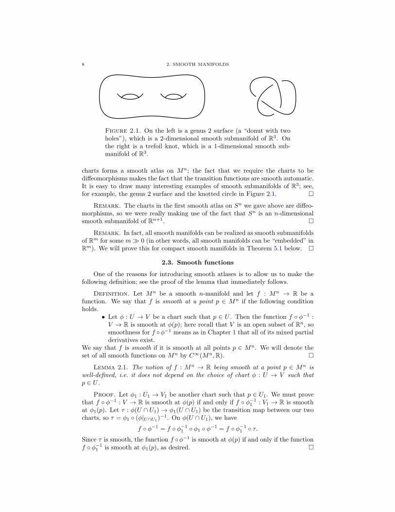
Figure 2.1. On the left is a genus 2 surface (a “donut with twoholes”), which is a 2-dimensional smooth submanifold of R3. Onthe right is a trefoil knot, which is a 1-dimensional smooth sub-manifold of R3.

charts forms a smooth atlas on Mn; the fact that we require the charts to bediffeomorphisms makes the fact that the transition functions are smooth automatic.It is easy to draw many interesting examples of smooth submanifolds of R3; see,for example, the genus 2 surface and the knotted circle in Figure 2.1. □

Remark. The charts in the first smooth atlas on Sn we gave above are diffeo-morphisms, so we were really making use of the fact that Sn is an n-dimensionalsmooth submanifold of Rn+1. □

Remark. In fact, all smooth manifolds can be realized as smooth submanifoldsof Rm for some m≫ 0 (in other words, all smooth manifolds can be “embedded” inRm). We will prove this for compact smooth manifolds in Theorem 5.1 below. □

2.3. Smooth functions

One of the reasons for introducing smooth atlases is to allow us to make thefollowing definition; see the proof of the lemma that immediately follows.

Definition. Let Mn be a smooth n-manifold and let f : Mn → R be afunction. We say that f is smooth at a point p ∈ Mn if the following conditionholds.

• Let ϕ : U → V be a chart such that p ∈ U . Then the function f ◦ ϕ−1 :V → R is smooth at ϕ(p); here recall that V is an open subset of Rn, sosmoothness for f ◦ϕ−1 means as in Chapter 1 that all of its mixed partialderivatives exist.

We say that f is smooth if it is smooth at all points p ∈ Mn. We will denote theset of all smooth functions on Mn by C∞(Mn,R). □

Lemma 2.1. The notion of f : Mn → R being smooth at a point p ∈ Mn iswell-defined, i.e. it does not depend on the choice of chart ϕ : U → V such thatp ∈ U .

Proof. Let ϕ1 : U1 → V1 be another chart such that p ∈ U1. We must provethat f ◦ ϕ−1 : V → R is smooth at ϕ(p) if and only if f ◦ ϕ−1

1 : V1 → R is smoothat ϕ1(p). Let τ : ϕ(U ∩ U1) → ϕ1(U ∩ U1) be the transition map between our twocharts, so τ = ϕ1 ◦ (ϕ|U∩U1)

−1. On ϕ(U ∩ U1), we have

f ◦ ϕ−1 = f ◦ ϕ−11 ◦ ϕ1 ◦ ϕ−1 = f ◦ ϕ−1

1 ◦ τ.Since τ is smooth, the function f ◦ϕ−1 is smooth at ϕ(p) if and only if the functionf ◦ ϕ−1

1 is smooth at ϕ1(p), as desired. □

2.3. SMOOTH FUNCTIONS 9

Definition. If f : Mn → R is a smooth function on Mn and ϕ : U → Vis a chart on Mn, then the smooth function f ◦ ϕ−1 : V → R will be called theexpression for f in the local coordinates V . □

Remark. IfMn is a smooth submanifold of Rm, then we now have two differentdefinitions of what it means for a function f :Mn → R to be smooth:

• The definition we just gave, and• The definition given right before the definition of a smooth submanifoldof Rm, i.e. a function f : Mn → R that can be extended to a smoothfunction g : U → R for some open set U ⊂ Rm containing Mn.

In the exercises, you will prove that these two definitions are equivalent. By theway, this makes it easy to write down many examples of smooth functions. Forexample, the function f : Sn → R defined via the formula

f(x1, . . . , xn+1) =

n+1∑i=1

ix2i+1i

is smooth; here we are regarding Sn as a smooth submanifold of Rn+1. □Defining what it means for a map between arbitrary manifolds to be smooth is

a little complicated. Consider the following example.

Example. Define a map f : R → S1 via the formula f(t) = (cos(t), sin(t)) ∈S1 ⊂ R2. We clearly want f to be smooth. Recall that R is endowed with thesmooth atlas with a single chart, namely the identity map R → R. The image ofthis chart under f is not contained in any single chart for S1, so we cannot definesmoothness for f locally using this smooth atlas. □

The problem with the above example is that we really need to use “smaller”charts on R. We now adapt the following convention to circumvent this.

Convention. If Mn is a smooth manifold with smooth atlas A, then we willautomatically enlarge A to the maximal atlas compatible with A (remember ourequivalence relation on smooth atlases!). In particular, if ϕ : U → V is a chart forMn, then so is ϕ|U ′ : U ′ → ϕ(U ′) for any open set U ′ ⊂ U . □

With this convention, we make the following definition.

Definition. Let f : Mn11 → Mn2

2 be a map between smooth manifolds. Wesay that f is smooth at a point p ∈Mn1

1 if there exist charts ϕ1 : U1 → V1 for Mn11

and ϕ2 : U2 → V2 for Mn22 with the following properties.

• p ∈ U1.• f(U1) ⊂ U2.• The composition

V1ϕ−11−−→ U1

f−→ U2ϕ2−→ V2

is smooth at ϕ1(p); this makes sense since V1 and V2 are open subsets ofRn1 and Rn2 , respectively.

We say that f is smooth if it is smooth at all points p ∈Mn11 . We will denote the set

of all smooth functions from Mn11 to Mn2

2 by C∞(Mn11 ,Mn2

2 ). A diffeomorphismis a smooth bijection whose inverse is also smooth. □

Just like for real-valued smooth functions, this does not depend on the choiceof charts.


Definition. If f : Mn11 → Mn2

2 is a smooth function between smooth mani-folds, ϕ1 : U1 → V1 is a chart for Mn1

1 , and ϕ2 : U2 → V2 is a chart for Mn22 such

that f(U1) ⊂ U2, then the smooth function V1 → V2 obtained as the composition

V1ϕ−11−−→ U1

f−→ U2ϕ2−→ V2

will be called the expression for f in the local coordinates V1 and V2. □

Example. It is immediate that the function f : R → S1 discussed abovedefined via the formula f(t) = (cos(t), sin(t)) ∈ S1 ⊂ R2 is smooth. □

Remark. Just as before, if M1 and M2 are smooth submanifolds of Euclideanspace this definition agrees with the definition given just before the definition ofsmooth submanifolds. This allows us to write down many interesting examples ofsmooth maps. For example, regarding S1 as a smooth submanifold of R2 we candefine a smooth map f : S1 → S1 via the formula f(x1, x2) = (x21 −x22, 2x1x2). □

2.4. Manifolds with boundary

The following spaces are not manifolds.

Example. The set Dn = {(x1, . . . , xn) ∈ Rn | x21 + · · ·+ x2n ≤ 1} is not a man-ifold since the points of Sn−1 ⊂ Dn do not have open neighborhoods in Dn homeo-morphic to open subsets of Rn. In particular, [0, 1] is not a manifold. □

However, Dn is an example of a manifold with boundary, which we now define.

Notation. Define

Hn = {(x1, . . . , xn) ∈ Rn | xn ≥ 0}and

∂Hn = {(x1, . . . , xn) ∈ Rn | xn = 0}. □

Definition. A smooth n-manifold with boundary is a Hausdorff paracompactspace Mn together with a smooth atlas {ϕi : Ui → Vi}i∈I , which is defined exactlylike for ordinary smooth manifolds except that now Vi is an open subset of Hn. □

There is one subtle aspect of the above definition: since Vi is an open subsetof Hn, we need to be careful about what it means for the transition functions to besmooth. The correct definition of a smooth function on an arbitrary (not necessarilyopen) subset of Rn is as follows.

Definition. Let X ⊂ Rn be arbitrary and let f : X → Rm be a function. Wesay that f is smooth if there exists an open set U ⊂ Rn such that X ⊂ U as well asa smooth function g : U → Rm such that g|X = f . □

Smooth maps between manifolds with boundary are defined exactly like thosebetween ordinary manifolds.

We now define the boundary of a smooth manifold with boundary.

Definition. Let Mn be a smooth manifold with boundary. The boundary ofMn, denoted ∂Mn, is the set of all points x ∈ Mn such that there exists a chartϕ : U → V with x ∈ U and V ⊂ Hn and ϕ(x) ∈ ∂Hn. The interior of Mn, denotedInt(Mn), is the set of all points x ∈ Mn such that there exists a chart ϕ : U → Vwith x ∈ U and V ⊂ Hn and ϕ(x) /∈ ∂Hn. □

2.4. MANIFOLDS WITH BOUNDARY 11

Figure 2.2. Removing the shaded submanifold of the genus 2surface results in a surface with boundary whose boundary consistsof the union of two circles.

Of course, with this definition it is not immediately obvious that ∂Mn is disjointfrom Int(Mn). However, the following lemma says that it is.

Lemma 2.2. Let Mn be a smooth manifold with boundary. Then ∂Mn ∩Int(Mn) = ∅.

Proof. To prove this, it is enough to prove that if U ⊂ Hn is an open set suchthat U ∩ ∂Hn = ∅, then there does not exist a diffeomorphism f : U → U ′, whereU ′ ⊂ Hn satisfies U ′ ∩ ∂Hn = ∅. Assume that such a diffeomorphism f : U → U ′

exists. By definition, we can find an open set V ⊂ Rn such that U = Hn ∩Vand a function g : V → Rn such that f = g|U . Let p ∈ U ∩ ∂Hn. Since f is adiffeomorphism, the derivative Dpg = Dpf is an isomorphism. By Theorem 5.2(the Implicit Function Theorem), the map g is a local diffeomorphism around p,i.e. there exists an open neighborhood V ′ of p such that V ′ ⊂ V and such that grestricts to a diffeomorphism between V ′ and an open set W in Rn. Since U ′ isopen in Rn (after all, it does not intersect ∂Hn), the set U ′∩W is open in Rn. Butthis implies that

g−1(U ′ ∩W ) = f−1(U ′ ∩W ) ⊂ Hn

is an open subset of Rn. Since f−1(U ′ ∩W ) contains the point p ∈ ∂Hn, this isimpossible, as desired. □

We now discuss some examples.

Example. Every smooth manifold is a smooth manifold with boundary. Thepoint is that every open subset of Rn is diffeomorphic to an open subset of Hn.The boundary of a smooth manifold is empty. □

Example. The set [0, 1] is a smooth 1-manifold with boundary and ∂[0, 1] is{0, 1}. □

We will later prove (see Theorem 11.1) that all compact connected 1-manifoldswith boundary are diffeomorphic to either S1 or [0, 1].

Example. More generally, Dn is a smooth n-manifold with boundary and∂Dn = Sn−1. This is not hard to prove directly, but we will derive it from moregeneral considerations in §5.6. □

Example. Our final example will be intuitively plausible, but we will not beable to justify it until Chapter 5 (where it will appear in the exercises). Let Mn

be a smooth n-manifold and let Xn be a smooth n-manifold with boundary thatis a smooth submanifold of Mn (we have not yet defined what this means, but we


hope that the idea is intuitively clear). Then Mn \ Int(Xn) is a smooth n-manifoldwith boundary and ∂(Mn \ Int(Xn)) = ∂Xn. As an example, see Figure 2.2. Thiskind of example shows one important role played by manifolds with boundary: theyappear during “cut-and-paste” operations on manifolds. □

2.5. Partitions of unity

We now introduce an important technical device. In calculus, we learned how toconstruct many interesting functions on open subsets of Rn. To use these functionsto prove theorems about manifolds, we need a tool for assembling local informationinto global information. This tool is called a smooth partition of unity, which wenow define. Recall that if f :Mn → R is a function, then the support of f , denotedSupp(f), is the closure of the set {x ∈Mn | f(x) = 0}.

Definition. Let Mn be a smooth manifold with boundary and let {Ui}i∈Ibe an open cover of Mn. A smooth partition of unity subordinate to {Ui}ki=1 is acollection of smooth functions {fi :Mn → R}i∈I satisfying the following properties.

• We have 0 ≤ fi(x) ≤ 1 for all 1 ≤ i ≤ k and x ∈Mn.• We have Supp(fi) ⊂ Ui for all 1 ≤ i ≤ k.• For all p ∈ Mn, there exists an open neighborhood W of p such that theset {i ∈ I | W ∩ Supp(fi) = ∅} is finite.

• For all p ∈ Mn, we have∑i∈I fi(p) = 1. This sum makes sense since

the previous condition ensures that only finitely many terms in it arenonzero. □

Theorem 2.3 (Existence of partitions of unity). Let Mn be a smooth manifoldwith boundary and let {Ui}i∈I be an open cover of Mn. Then there exists a smoothpartition of unity subordinate to {Ui}i∈I .

For the proof of Theorem 2.3, we need the following lemma.

Lemma 2.4 (Bump functions, weak). LetMn be a smooth manifold with bound-ary, let p ∈ Mn be a point, and let U ⊂ Mn be a neighborhood of p. Then thereexists a smooth function f :Mn → R such that 0 ≤ f(x) ≤ 1 for all x ∈Mn, suchthat f equals 1 in some neighborhood of p, and such that Supp(f) ⊂ U .

Proof. We will construct f in a sequence of steps.

Step 1. There exists a smooth function g : R → R such that 0 ≤ g(x) ≤ 1 forall x ∈ R, such that g(x) = 1 when |x| ≤ 1, and such that Supp(g) ⊂ (−3, 3).

Define g1 : R → R via the formula

g1(x) =

{0 if x ≤ 0,

e−1/x if x > 0.(x ∈ R).

The function g1 is a smooth function such that g1(x) ≥ 0 for all x ∈ R, suchthat g1(x) = 0 when x ≤ 0, and such that g1(x) > 0 when x > 0. Next, defineg2 : R → R via the formula

g2(x) =g1(x)

g1(x) + g1(1− x),

so g2 is a smooth function such that 0 ≤ g2(x) ≤ 1 for all x ∈ R, such that g2(x) = 0when x ≤ 0, and such that g2(x) = 1 when x ≥ 1. Finally, define g via the formula

g(x) = g1(2 + x)g1(2− x).

2.5. PARTITIONS OF UNITY 13

Clearly g satisfies the desired conditions.

Step 2. Let C0 = {x ∈ Rn | ∥x∥ ≤ 1} and U0 = {x ∈ Rn | ∥x∥ < 2}. Thenthere exists a smooth function h : Rn → R such that 0 ≤ h(x) ≤ 1 for all x ∈ Rn,such that h|C0 = 1, and such that Supp(h) ⊂ U0.

Let g be as in Step 1. Define h via the formula

h(x1, . . . , xn) = g(x21 + · · ·+ x2n).

Clearly h satisfies the desired conditions.

Step 3. There exists a smooth function f as in the statement of the lemma.

Let C0 and U0 and h be as in Step 2. We can then find an open set U ′ ⊂ U suchthat p ∈ U ′ and a diffeomorphism ϕ : U ′ → V , where V is either an open subset ofRn containing U0 or an open subset of Hn containing U0 ∩ Hn and ϕ(p) = 0. Thefunction f :Mn → R can then be defined via the formula

f(x) =

{g(ϕ(x)) if x ∈ U ′,

0 otherwise.(x ∈Mn).

Clearly f satisfies the conditions of the lemma. □

Proof of Theorem 2.3. Since Mn is paracompact and locally compact, wecan find open covers {U ′

j}j∈J and {U ′′j }j∈J of Mn with the following properties.

• The cover {U ′j}j∈J refines the cover {Ui}i∈I , i.e. for all j ∈ J there exists

some ij ∈ I such that the closure of U ′j is contained in Uij .

• The cover {U ′j}j∈J is locally finite, i.e. for all p ∈ Mn there exists some

open neighborhood W of p such that {j ∈ J | W ∩ U ′j = ∅} is finite.

• The closure of U ′′j is a compact subset of U ′

j for all j ∈ J .For each p ∈ Mn, choose jp such that p ∈ U ′′

jpand use Lemma 2.4 to find a

smooth function gp : Mn → R such that 0 ≤ gp(x) ≤ 1 for all x ∈ Mn, such thatSupp(gp) ⊂ U ′

jp, and such that gp equals 1 in some neighborhood Vp of p. Since the

closure of U ′′j in U ′

j is compact for all j ∈ J , we can find a set {pk}k∈K of pointsof Mn such that the set {Vpk | k ∈ K, jpk = j} is a finite cover of U ′′

j for all j ∈ J .For all j ∈ J , define hj : M

n → R to be the sum of all the gpk such that jpk = j(a finite sum), so hj is a smooth function such that hj(x) ≥ 0 for all x ∈Mn, suchthat hj(x) > 0 for all x ∈ U ′′

j , and such that Supp(hj) ⊂ U ′j . Finally, for all i ∈ I,

define fi :Mn → R via the formula

fi(x) =

∑ij=i

hj(x)∑j∈J hj(x)

(x ∈Mn).

These are not finite sums, but because the cover {U ′j}j∈J is locally finite and

Supp(hj) ⊂ U ′j for all j ∈ J , only finitely many terms in each are nonzero for

any choice of x ∈ Mn and the numerator and denominator are smooth functions.Also, the denominator is nonzero since hj(x) > 0 for all x ∈ U ′′

j and the set {U ′′j }j∈J

is a cover.By construction, we have Supp(fi) ⊂ Ui. Moreover, for all x ∈Mn the fact that

the cover {U ′j}j∈J is locally finite and Supp(hj) ⊂ U ′

j for all j ∈ J implies that thereexists some open neighborhoodW of x such that the set {i ∈ I | W ∩ Supp(fi) = ∅}


is finite. Finally, for all x ∈Mn we have∑i∈I

fi(x) =

∑i∈I

∑ij=i

hj(x)∑j∈J hj(x)

=

∑j∈J hj(x)∑j∈J hj(x)

= 1,

as desired. □

As a first illustration of how Theorem 2.3 can be used, we prove the followinglemma.

Lemma 2.5 (Bump functions, strong). Let Mn be a smooth manifold withboundary, let C ⊂ Mn be a closed set, and let U ⊂ Mn be an open set such thatC ⊂ U . Then there exists a smooth function f : Mn → R such that 0 ≤ f(x) ≤ 1for all x ∈Mn, such that f(x) = 1 for all x ∈ C, and such that Supp(f) ⊂ U .

Proof. Set U ′ =Mn \C. The set {U,U ′} is then an open cover ofMn. UsingTheorem 2.3, we can find smooth functions f :Mn → R and g :Mn → R such that0 ≤ f(x), g(x) ≤ 1 for all x ∈ Mn, such that Supp(f) ⊂ U and Supp(g) ⊂ U ′, andsuch that f + g = 1. The function f then satisfies the conditions of the lemma. □

This has the following useful consequence. Just like for functions on Euclideanspace, if C is an arbitrary subset of a smooth manifold M1 and f : C → M2 is afunction to another smooth manifold, then f is said to be smooth if there existsan open set U ⊂ M1 containing C and a smooth function g : U → M2 such thatg|C = f .

Lemma 2.6 (Extending smooth functions). Let M be a smooth manifold withboundary, let C ⊂ M be a closed set, and let U ⊂ M be an open set such thatC ⊂ U . Let f : C → R be a smooth function. Then there exists a smooth functiong :M → R such that g|C = f and such that Supp(g) ⊂ U .

Proof. By definition, there exists an open set U ′ ⊂ M containing C and asmooth function g1 : U ′ → R such that g1|C = f . Shrinking U ′ if necessary, we canassume that U ′ ⊂ U . Use Lemma 2.5 to construct a smooth function h : M → Rsuch that 0 ≤ h(x) ≤ 1 for all x ∈ M , such that h(x) = 1 for all x ∈ C, and suchthat Supp(h) ⊂ U ′. Define g :M → R via the formula

g(x) =

{h(x)g1(x) if x ∈ U ′,

0 otherwise.(x ∈M).

Clearly g satisfies the conclusions of the lemma. □

2.6. Approximating continuous functions, I

As another illustration of how partitions of unity can be used, we will provethe following.

Theorem 2.7. Let Mn be a smooth manifold with boundary and let f :Mn →Rm be a continuous function. Then for all ϵ > 0 there exists a smooth functiong :Mn → Rm such that ∥f(x)− g(x)∥ < ϵ for all x ∈Mn.

Remark. If Mn is not compact, then it is often useful to require that ∥f(x)−g(x)∥ < ϵ(x) for all x ∈ Mn, where ϵ : Mn → R is a fixed function such thatϵ(x) > 0 for all x ∈Mn. The proof is exactly the same. □

2.6. APPROXIMATING CONTINUOUS FUNCTIONS, I 15

Remark. We will later use an important tool called the tubular neighborhoodtheorem to generalize Theorem 2.7 to show that continuous functions between ar-bitrary smooth manifolds can be approximated in an appropriate sense by smoothfunctions; see Theorem 6.5. □

For the proof of Theorem 2.7, we need the following lemma.

Lemma 2.8. Let U ⊂ Rn be an open set and let f : U → Rm be a continuousfunction such that Supp(f) ⊂ U . Then for all ϵ > 0 there exists a smooth functiong : U → Rm such that Supp(g) ⊂ U and such that ∥f(x)−g(x)∥ < ϵ for all x ∈Mn.

Proof. The Stone-Weierstrass theorem says that we can find a smooth func-tion g1 : U → Rm such that ∥f(x) − g1(x)∥ < ϵ for all x ∈ U (in fact, it saysthat we can take g1 to be a function whose coordinate functions are polynomi-als). Let C = Supp(f), so C is a closed subset of U . Using Lemma 2.5, we canfind a smooth function β : U → R such that 0 ≤ β(x) ≤ 1 for all x ∈ U , suchthat β|C = 1, and such that Supp(β) ⊂ U . Define g : U → Rm via the formulag(x) = β(x) · g1(x). Since Supp(β) ⊂ U , we also have Supp(g) ⊂ U . Also, weclearly have ∥f(x)− g(x)∥ < ϵ for all x ∈ C. For x ∈ U \ C, we have f(x) = 0, so∥g1(x)∥ < ϵ and hence

∥f(x)− g(x)∥ = ∥β(x) · g1(x)∥ ≤ ∥g1(x)∥ < ϵ,

as desired. □

Proof of Theorem 2.7. In the exercises, you will construct a smooth atlasA = {ϕi : Ui → Vi}i∈I for Mn and a large integer K such that for all p ∈ Mn,there exists a neighborhood W of p with |{i ∈ I | Ui ∩W = ∅}| < K. We remarkthat this is trivial if Mn is compact. Using Theorem 2.3, we can find a smoothpartition of unity {νi : Ui → R}i∈I subordinate to {Ui}i∈I . Define fi : M

n → Rmvia the formula fi(x) = νi(x) · f(x). We thus have∑

i∈I

fi(x) = (∑i∈I

νi(x)) · f(x) = f(x) (x ∈Mn).

These sums makes sense since only finitely many terms in them are nonzero for

any fixed x ∈ Mn. Moreover, Supp(fi) ⊂ Ui. Define fi : Vi → Rm to be the

expression for fi in the local coordinates Vi, so fi = f ◦ϕ−1i . Applying Lemma 2.8,

we can find a smooth function gi : Vi → Rm such that Supp(gi) ⊂ Vi and such that

∥fi(x)− gi(x)∥ < ϵ/K for all x ∈ Vi. Define gi :Mn → Rm via the formula

gi(x) =

{gi(ϕi(x)) if x ∈ Ui,

0 otherwise(x ∈Mn).

Since Supp(gi) ⊂ Vi, this is a smooth function on Mn satisfying Supp(gi) ⊂ Ui.Moreover, ∥fi(x) − gi(x)∥ < ϵ/K for all x ∈ Mn. Define g : Mn → Rm via theformula

g(x) =∑i∈I

gi(x) (x ∈Mn);

this makes sense because Supp(gi) ⊂ Ui, and hence only finitely many terms in thissum are nonzero for any fixed x ∈Mn. The function g is a smooth function and

∥f(x)− g(x)∥ = ∥∑i∈I

(fi(x)− gi(x))∥ ≤∑i∈I

∥fi(x)− gi(x)∥ < K(ϵ/K) = ϵ,


as desired. □The following “relative” version of Theorem 2.7 will also be useful.

Theorem 2.9. Let Mn be a smooth manifold with boundary and let f :Mn →Rm be a continuous function. Assume that f |U is smooth for some open set U .Then for all ϵ > 0 and all closed sets C ⊂ Mn with C ⊂ U , there exists a smoothfunction g : Mn → Rm such that ∥f(x) − g(x)∥ < ϵ for all x ∈ Mn and such thatg|C = f |C .

Proof. The proof is very similar to the proof of Theorem 2.7, so we onlydescribe how it differs. The key is to choose the smooth atlas A = {ϕi : Ui → Vi}i∈Ifor Mn at the beginning of the proof such that if Ui ∩ C = ∅ for some i ∈ I, thenUi ⊂ U . For i ∈ I with Ui ⊂ U , we can then take our “approximating functions”

gi to simply equal fi, and thus gi = fi. These choices ensure that the functiong : Mn → Rm constructed in the proof of Theorem 2.7 satisfies g|C = f |C , asdesired. □

CHAPTER 3

The tangent bundle

In this chapter, we will construct the tangent bundle of a smooth manifold anddescribe how to differentiate smooth functions. We will then discuss vector fieldsand show how then can be integrated to flows. Finally, as an application we willprove that if M is a smooth manifold and p, q ∈ M are points, then there exists adiffeomorphism f :M →M such that f(p) = q.

3.1. Tangent spaces

Let Mn be a smooth n-manifold and let p ∈Mn. Our first goal is to constructan n-dimensional vector space TpM

n called the tangent space to Mn at p. Ifϕ : U → V is a chart around p, then vectors in TpM

n should be represented byelements of Tϕ(p)V = Rn. To make a definition that does not depend on anyparticular choice of chart, we introduce the following equivalence relation.

Definition. Let Mn be a smooth n-manifold, let p ∈Mn, and let {ϕi : Ui →Vi}i∈I be the set of charts around p. For i, j ∈ I, let τji : ϕi(Ui∩Uj) → ϕj(Ui∩Uj)be the transition function from Ui to Uj . Finally, let X (Mn, p) be the set of pairs(i, v), where i ∈ I and v ∈ Tϕi(p)Vi. Define ∼ to be the relation on X (Mn, p) wherewhere (i, v) ∼ (j, w) when (Dϕi(p)τji)(v) = w. □

Lemma 3.1. The relation ∼ defined in the previous definition is an equivalencerelation on X (Mn, p).

Proof. We must check reflexivity, symmetry, and transitivity.For (i, v) ∈ X (Mn, p), we have (i, v) ∼ (i, v) since the relevant transition

function τii : ϕi(Ui ∩ Ui) → ϕi(Ui ∩ Ui) is the identity.If (i, v), (j, w) ∈ X (Mn, p) satisfy (i, v) ∼ (j, w), then by definition we have

(Dϕi(p)τji)(v) = w. From its definition, we see that τij : ϕj(Ui ∩Uj) → ϕi(Ui ∩Uj)is the inverse of τji : ϕi(Ui ∩ Uj) → ϕj(Ui ∩ Uj). From Theorem 1.1 (the ChainRule I), we have (Dϕj(p)τij) ◦ (Dϕi(p)τji) = id, so (Dϕj(p)τij)(w) = v and hence(j, w) ∼ (i, v).

If (i, v), (j, w), (k, u) ∈ X (Mn, p) satisfy (i, v) ∼ (j, w) and (j, w) ∼ (k, u),then by definition we have (Dϕi(p)τji)(v) = w and (Dϕj(p)τkj)(w) = u. From itsdefinition, we see that on ϕi(Ui ∩ Uj ∩ Uk) we have τki = τkj ◦ τji. Again usingTheorem 1.1 (the Chain Rule I), we see that Dϕi(p)τki = (Dϕj(p)τkj) ◦ (Dϕi(p)τji),so (Dϕi(p)τki)(v) = u and hence (i, v) ∼ (k, u). □

This allows us to make the following definition.

Definition. Let Mn be a smooth manifold and let p ∈ Mn. Let {ϕi : Ui →Vi}i∈I be the set of charts around p. The tangent space to Mn at p, denoted TpM

n,is the set of equivalence classes of elements of X (Mn, p) under the equivalencerelation given by Lemma 3.1. □

17

18 3. THE TANGENT BUNDLE

Lemma 3.2. Let Mn be a smooth manifold and let p ∈Mn. Then the tangentspace TpM

n is an n-dimensional vector space.

Proof. This follows from the fact that the derivatives used to define the equiv-alence relation are vector space isomorphisms, so the vector space structures onthe various Tϕi(p)Vi used to define TpM

n descend to a vector space structure onTpM

n. □Convention. The notation X (Mn, p) that we used when defining TpM

n willnot be used again. In the future, instead of talking about elements of TpM

n beingequivalence classes of pairs (i, v), we will simply say that a given element of TpM

n

is represented by some v ∈ Tϕi(p)Vi. □

3.2. Derivatives I

Let f : Mn11 → Mn2

2 be a smooth map between smooth manifolds and letp ∈Mn1

1 . We now show how to construct the derivative Dpf : TpMn11 → Tf(p)M

n22 ,

which is a linear map between these vector spaces. Let ϕ1 : U1 → V1 be a chartaround p and let ϕ2 : U2 → V2 be a chart around ϕ(p) such that f(U1) ⊂ U2. Wethus have identifications TpM

n11 = Tϕ1(p)V1 and Tf(p)M

n22 = Tϕ2(f(p))V2. We define

Dpf : TpMn11 → Tf(p)M

n22 to be composition

TpMn11

=−→ Tϕ1(p)V1Dϕ1(p)(ϕ2◦f◦ϕ−1

1 )−−−−−−−−−−−−→ Tϕ2(f(p))V2

=−→ Tf(p)Mn22 .

Lemma 3.3. This does not depend on the choice of charts.

Proof. This is in the exercises; it provides good practice in the various iden-tifications we have made. □

Theorem 1.1 (the Chain Rule I) immediately implies the following version ofthe chain rule.

Theorem 3.4 (Manifold Chain Rule I). Let f : Mn11 → Mn2

2 and g : Mn22 →

Mn33 be smooth maps between smooth manifolds. Then for all p ∈Mn1

1 we have

Dp(g ◦ f) = (Df(p)g) ◦ (Dpf).

3.3. The tangent bundle

Let Mn be a smooth manifold. The goal of this section is to construct thetangent bundle of Mn. Recall that if V ⊂ Rn is an open subset, then TV =V × Rn. This contains all the individual tangent spaces TpV for p ∈ V , namelyTpV = {p} × Rn ⊂ TV . We wish to do a similar thing with the tangent spacesTpM

n for p ∈Mn. The result will be a 2n-dimensional smooth manifold TMn.Just like for the tangent spaces, we will define TMn using an equivalence rela-

tion.

Definition. Let Mn be a smooth n-manifold with smooth atlas {ϕi : Ui →Vi}i∈I . For i, j ∈ I, let τji : ϕi(Ui ∩ Uj) → ϕj(Ui ∩ Uj) be the transition functionfrom Ui to Uj . Finally, let Y(Mn) be the set of triples (i, p, v), where i ∈ I andp ∈ Ui and v ∈ Tϕi(p)Vi. Define ∼ to be the relation on Y(Mn) where (i, p, v) and(j, q, w) satisfy (i, p, v) ∼ (j, q, w) when p = q and (Dpτji)(v) = w. □

Lemma 3.5. The relation ∼ defined in the previous definition is an equivalencerelation on Y(Mn).

3.5. VISUALIZING THE TANGENT BUNDLE 19

Proof. Immediate from Lemma 3.1. □

This allows us to make the following definition.

Definition. Let Mn be a smooth manifold with smooth atlas {ϕi : Ui →Vi}i∈I . The tangent bundle of Mn, denoted TMn, is the set of equivalence classesof elements of Y(Mn) under the equivalence relation given by Lemma 3.5. □

We can identify Y(Mn) with the disjoint union of all the TVi by identifying(i, p, v) with (ϕi(p), v) ∈ TVi. This endows Y(Mn) with a topology. We give TMn

the quotient topology, so by definition, a set U ⊂ TMn is open if its preimageunder the projection

Y(Mn)mod ∼−−−−→ TMn

is open. Under this projection, each TVi maps injectively into TMn; as temporarynotation, let its image be TVi ⊂ TMn. Since TVi = Vi × Rn is an open subset ofR2n = Rn × Rn and there is an evident (and trivial) homeomorphism ψi : TVi →TVi, we deduce that TMn is a manifold. Even better, the set {ψi : TVi → TVi}i∈Iis a smooth atlas: the transition function from TVi to TVj equals the derivativeDτji : Tϕi(Ui ∩ Uj) → Tϕj(Ui ∩ Uj) of the transition function τji : ϕi(Ui ∩ Uj) →ϕj(Ui ∩ Uj), which is clearly smooth. We have proved the following theorem.

Theorem 3.6. LetMn be a smooth n-manifold. Then the tangent bundle TMn

of Mn is a smooth 2n-dimensional manifold.

Convention. Just like for the tangent space, we will never again use thenotation Y(Mn) or the formalism of triples (i, p, v) when discussing TMn. Instead,we will say that a given point of TMn is represented by a given point of TVi. □

Remark. See §3.5 for a discussion of how to visualize the tangent bundle. □

3.4. Derivatives II

If f :M1 →M2 is a smooth map between smooth manifolds, then we previouslyhave defined linear maps Dpf : TpM1 → Tf(p)M2 for all p ∈ M1. These piecetogether to define a map Df : TM1 → TM2 that restricted to the subspace TpM1

of TM1 equals Dpf . It is clear that this is a smooth map. Just like for Theorem1.2 (Chain Rule II), Theorem 3.4 implies the following.

Theorem 3.7 (Manifold Chain Rule II). Let f : Mn11 → Mn2

2 and g : Mn22 →

Mn33 be smooth maps between smooth manifolds. Then

D(g ◦ f) = (Dg) ◦ (Df).

3.5. Visualizing the tangent bundle

Our construction of the tangent bundle was very abstract. In the case ofsmooth submanifolds of Rm, there is a simpler construction which is a great aidto visualization. Consider a smooth submanifold Mn ⊂ Rm. For p ∈ Mn, we canregard TpM

n as a subspace of TpRm = Rm in the following way. By definition,there is a diffeomorphism ϕ : U → V , where U ⊂ Mn is an open neighborhood ofp and V ⊂ Rn is an open set. The inverse ϕ−1 can be regarded as a smooth mapfrom V to Rm, and thus it has a derivative

Dϕ(p)ϕ−1 : Tϕ(p)V → TpRm = Rm.


p

v∈TpS1

Figure 3.1. A vector v ∈ TpS1 is orthogonal to the line from 0 to p.

The image of this derivative can be identified with the tangent space TpMn; it is

easy to see that it does not depend on the choice of diffeomorphism ϕ : U → V .Using this, we can regard the tangent bundle TMn as the subspace

{(p, v) ∈ TRm | p ∈Mn, v ∈ TpMn ⊂ TpRm} ⊂ TRm = Rm × Rm.

This results in the familar picture of tangent vectors to Mn as being arrows in Rmthat “point in the direction of the tangent plane to Mn”.

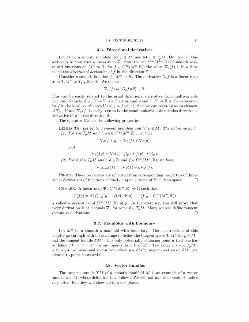
Example. For Sn ⊂ Rn+1, you will prove in the exercises that

TSn = {(p, v) ∈ TRn+1 | ∥p∥ = 1 and v is orthogonal to the line from 0 to p}.

See Figure 3.1. □

The derivative map can also be understood from this perspective. Let Mn11 ⊂

Rm1 and Mn22 ⊂ Rm2 be smooth submanifolds of Euclidean space and let f :

Mn11 → Mn2

2 be a smooth map. By definition, this means that there exists anopen set U ⊂ Rm1 and a smooth map g : U → Rm2 such that g|Mn1

1= f . As

discussed in Chapter 1 (our review of multivariable calculus), the map g induces aderivative map Dg : TU → TRm2 ; on TpU ⊂ TU for p ∈ U , this is just the linearderivative map Dpg : TpU → Tg(p)Rm2 . The derivative Df : TMn1

1 → TMn22 is

then just the restriction of Dg to TMn11 ⊂ TU ; this image of this restriction lies in

TMn22 ⊂ TRm2 .Often the smooth map f : Mn1

1 → Mn22 is given by a formula which can be

extended to an open set U (often all of Rm1 , or at least Rm1 minus some isolatedpoints where the formula has a singularity). Using this formula, it is easy to usethe above recipe to work out the effect of Df .

3.8. VECTOR BUNDLES 21

3.6. Directional derivatives

Let M be a smooth manifold, let p ∈ M , and let v ∈ TpM . Our goal in thissection is to construct a linear map ∇v from the set C∞(Mn,R) of smooth real-valued functions on Mn to R; for f ∈ C∞(Mn,R), the value ∇v(f) ∈ R will becalled the directional derivative of f in the direction v.

Consider a smooth function f : Mn → R. The derivative Dpf is a linear mapfrom TpM

n to Tf(p)R = R. We define

∇v(f) = (Dpf)(v) ∈ R.

This can be easily related to the usual directional derivative from multivariablecalculus. Namely, if ϕ : U → V is a chart around p and g : V → R is the expressionfor f in the local coordinates V (so g = f ◦ϕ−1), then we can regard v as an elementof Tϕ(p)V and ∇v(f) is easily seen to be the usual multivariable calculus directionalderivative of g in the direction v.

The operator ∇v has the following properties.

Lemma 3.8. Let M be a smooth manifold and let p ∈M . The following hold.(1) For v ∈ TpM and f, g ∈∈ C∞(Mn,R), we have

∇v(f + g) = ∇v(f) +∇v(g)

and

∇v(fg) = ∇v(f) · g(p) + f(p) · ∇v(g).

(2) For v, w ∈ TpM and c, d ∈ R and f ∈ C∞(Mn,R), we have

∇cv+dw(f) = c∇v(f) + d∇w(f).

Proof. These properties are inherited from corresponding properties of direc-tional derivatives of functions defined on open subsets of Euclidean space. □

Remark. A linear map Ψ : C∞(Mn,R) → R such that

Ψ(fg) = Ψ(f) · g(p) + f(p) ·Ψ(g) (f, g ∈ C∞(Mn,R))

is called a derivation of C∞(Mn,R) at p. In the exercises, you will prove thatevery derivation Ψ at p equals ∇v for some v ∈ TpM . Many sources define tangentvectors as derivations. □

3.7. Manifolds with boundary

Let Mn be a smooth n-manifold with boundary. The constructions of thischapter go through with little change to define the tangent space TpM

n for p ∈Mn

and the tangent bundle TMn. The only potentially confusing point is that one hasto define TV = V × Rn for any open subset V of Hn. The tangent space TpM

n

is thus an n-dimensional vector even when p ∈ ∂Mn; tangent vectors on ∂Mn areallowed to point “outwards”.

3.8. Vector bundles

The tangent bundle TM of a smooth manifold M is an example of a vectorbundle over M , whose definition is as follows. We will not use other vector bundlesvery often, but they will show up in a few places.


Definition. Let X be a topological space. A k-dimensional vector bundle overX is a topological space E together with a continuous map π : E → X such thatthe following hold for all all x ∈ X.

• The preimage π−1(x) is equipped with the structure of a k-dimensionalvector space. We will denote this vector space by Ex.

• There exists an open neighborhood U ⊂ X of x and a homeomorphismψ : U ×Rk → π−1(U) such that for all y ∈ U , we have ψ({y} ×Rk) = Eyand the composition

Rk∼=−→ {y} × Rk ψ−→ Ey

is a vector space isomorphism.The second condition is called local triviality. If X and E are smooth manifoldsand both π : E → X and all the isomorphisms ψ appearing above are smooth, thenE is a smooth vector bundle. □

Example. Let Mn be an n-dimensional smooth manifold. The projectionπ : TMn → Mn taking TpM

n to p makes TMn into a smooth n-dimensionalvector bundle overMn. Indeed, the preimage π−1(Mn) is the n-dimensional vectorspace TpM

n. Moreover, by definition for every chart ϕ : U → V of Mn we haveπ−1(U) ∼= TV ∼= V × Rn. □

Example. If X is a topological space, then E = X × Rk is a k-dimensionalvector bundle over X whose map π : E → X is simply the projection onto the firstfactor. This will be called the trivial k-dimensional vector bundle over X. If X isa smooth manifold, then this is a smooth vector bundle. □

The vector bundles that we will use will all be built out of the tangent bundleusing linear-algebraic operations. Rather than prove a general theorem about suchoperations, we will give several examples.

Construction. Fix a topological space X, and for i = 1, 2, let πi : Ei → Xbe a ki-dimensional vector bundle over X. Define

E1 ⊕ E2 = {(e1, e2) ∈ E1 × E2 | π(e1) = π(e2)}and let ρ : E1 ⊕E2 → X be the map taking (e1, e2) to π(e1). You will prove in theexercises that ρ : E1⊕E2 → X is a (k1+k2)-dimensional vector bundle over X suchthat for x ∈ X the vector space (E1 ⊕ E2)x is the vector space (E1)x ⊕ (E2)x. □

Construction. Let π : E → X be a k-dimensional vector bundle. Define

E∗ = {(x, τ) | x ∈ X and τ : Ex → R is a linear map}and let ρ : E∗ → X take (x, τ) to x. You will prove in the exercises that ρ : E∗ → Xis a k-dimensional vector bundle over X such that for x ∈ X the fiber (E∗)x is thedual vector space (Ex)

∗. This is called the dual bundle to X. The dual bundle ofthe tangent bundle of a smooth manifold M is the cotangent bundle and is denotedT ∗M . □

Construction. Let π : E → X be a k-dimensional vector bundle. Define

∧iE = {(x, v) | x ∈ X and v ∈ ∧iEx}and let ρ : E∗ → X take (x, v) to x. You will prove in the exercises that ρ : ∧iE →X is a

(ki

)-dimensional vector bundle over X such that for x ∈ X the fiber (∧iE)x

is the wedge product ∧iEx. □

3.8. VECTOR BUNDLES 23

Remark. All of the above constructions take smooth vector bundles to smoothvector bundles. □

Maps between vector bundles are defined as follows.

Definition. A vector bundle map between vector bundles π1 : E1 → X1 andπ2 : E2 → X2 is a pair of continuous maps f : X1 → X2 and g : E1 → E2 with thefollowing two properties.

• We have π2 ◦ g = f ◦ π1, i.e. the diagram

E1g−−−−→ E2

π1

y yπ2

X1f−−−−→ X2

commutes.• The previous condition implies that for x ∈ X1, the map g restricts to amap from the vector space (E1)x to the vector space (E2)x. We requirethat this map be linear.

If X1 = X2 = X and f = id, then we say that this is a vector bundle map over X.We will often not write f and simply say that g : E1 → E2 is a vector bundle map.If g : E1 → E2 is a bijective map of vector bundles over X and g−1 is continuous,then we will call g an isomorphism. □

Example. If f : M1 → M2 is a smooth map between smooth manifolds, thenthe derivative Df : TM1 → TM2 is a vector bundle map. □

This allows us to define our final four vector bundle operations.

Construction. For i = 1, 2, let πi : Ei → X be a ki-dimensional vectorbundle and let g : E1 → E2 be a vector bundle map over X. Assume that thevector space map (E1)x → (E2)x induced by g is surjective for all x ∈ X. Defineker(g) to be the set of pairs

{(x, v) | x ∈ X and v lies in the kernel of the map (E1)x → (E2)x induced by g}and let ρ : ker(g) → X to be the map taking (x, v) to x. You will prove in theexercises that ρ : ker(g) → X is a (k1 − k2)-dimensional vector bundle over X suchthat for x ∈ X the fiber ker(g)x is the kernel of the map (E1)x → (E2)x inducedby g. □

Construction. For i = 1, 2, let πi : Ei → X be a ki-dimensional vectorbundle and let g : E1 → E2 be a vector bundle map over X. Assume that thevector space map (E1)x → (E2)x induced by g is injective for all x ∈ X. Definecoker(g) to be the set of pairs

{(x, v) | x ∈ X and v lies in the quotient vector space (E2)x/g((E1)x)}and let ρ : coker(g) → X to be the map taking (x, v) to x. You will prove in theexercises that ρ : coker(g) → X is a (k2 − k1)-dimensional vector bundle over Xsuch that for x ∈ X the fiber coker(g)x is the quotient (E2)x/g((E1)x). □

Construction. Let π : E → X be a k-dimensional vector bundle and letf : Y → X be a continuous map. Define

f∗(E) = {(y, e) | y ∈ Y , e ∈ E, f(y) = π(e)} ⊂ Y × E.


The projection Y ×E → Y restricts to a map f∗(π) : f∗(E) → Y . In the exercises,you will prove that f∗(E) is a k-dimensional vector bundle with f∗(E)y = Ef(y)for all y ∈ Y . This fits into a map of vector bundles

f∗(E) −−−−→ E

f∗(π)

y yπY

f−−−−→ Xwhere the top row is the restriction of the projection Y × E → E. We will callf∗(E) the pull-back of E along f . □

Example. IfX is a topological space, X×Rk is the trivial k-dimensional vectorbundle, and f : Y → X is any continuous map, then f∗(X × Rk) is isomorphic asa vector bundle over Y to the trivial k-dimensional vector bundle Y ×Rk. Indeed,by definition we have

f∗(X × Rk) = {(y, (x, v)) ∈ Y × (X × Rk) | y ∈ Y };the vector bundle isomorphism simply takes (y, (x, v)) ∈ f∗(X × Rk) to (y, v) ∈Y × Rk. □

Construction. If X is a topological space, π : E → X is a vector bundle, andY ⊂ X is a subspace, then the restriction of E to Y , denoted E|Y , is the pullbackof E along the inclusion map Y ↪→ X. □

Remark. Again, all of the above constructions take smooth vector bundles tosmooth vector bundles. □

CHAPTER 4

Vector fields

In this chapter, we discuss some basic results about vector fields, including theirintegral curves and flows. As an application, we will prove that ifMn is a connectedsmooth manifold and p, q ∈Mn, then there exists a diffeomorphism f :Mn →Mn

such that f(p) = q.

4.1. Definition and basic examples

Let Mn be a smooth manifold with boundary. Intuitively, a smooth vectorfield on Mn is a smoothly varying choice of vector TpM

n for each p ∈ Mn. Moreprecisely, a smooth vector field on Mn is a smooth map ν : Mn → TMn suchthat ν(p) ∈ TpM

n for all p ∈ Mn. Let X(Mn) be the set of smooth vector fieldson Mn. The vector space structures on each TpM

n together endow X(Mn) withthe structure of a real vector space (infinite dimensional unless Mn is a compact0-manifold).

If ν ∈ X(Mn) and ϕ : U → V is a chart onMn, then the expression for ν in thelocal coordinates V is the function η : V → Rn such that η(ϕ(p)) ∈ Tϕ(p)V = Rnrepresents ν(p) for all p ∈ U .

It is particularly easy to write down smooth vector fields on smooth subman-ifolds Mn of Rm. Namely, recall that the embedding of Mn in Rm identifieseach TpM

n with an n-dimensional subspace of TRm = Rm. A smooth vectorfield on Mn can thus be identified with a smooth map ν : Mn → Rm such thatν(p) ∈ TpM

n ⊂ Rm for each p ∈ Mn. We warn the reader that this is differentfrom the expressions for ν in local coordinates defined above.

Example. Consider an odd-dimensional sphere S2n−1 ⊂ R2n. Recall that

TS2n−1 = {(p, v) ∈ TR2n | ∥p∥ = 1 and v is orthogonal to the line from 0 to p}.

We can then define a smooth vector field on S2n−1 via the formula

ν(x1, . . . , x2n) = (x2,−x1, x4,−x3, . . . , x2n,−x2n−1) ∈ T(x1,...,x2n)S2n−1 ⊂ Rm

for each (x1, . . . , x2n) ∈ S2n−1. The smooth vector field ν has the property thatν(p) = 0 for all p ∈ S2n−1. We will later prove the “hairy ball theorem”, whichasserts that no such nonvanishing smooth vector field exists on an even-dimensionalsphere. See Theorem 14.1. □

Example. Let Mn be a smooth submanifold of Rm and let f :Mn → R be asmooth function. We can then define a smooth vector field grad(f) on Mn in thefollowing way. Consider p ∈ Mn. We can define a linear map ηp : TpM

n → R viathe formula

ηp(v) = Xv(f).

25

26 4. VECTOR FIELDS

This is linear because of the second conclusion of Lemma 3.8. Let ω(·, ·) be theusual inner product on Rm. There then exists a unique vector grad(f)(p) ∈ TpM

n

such that

ηp(v) = ω(grad(f)(p), v) (v ∈ TpMn).

It is easy to see that this map grad(f) :Mn → TMn is a smooth vector field. □

Remark. In the construction of grad(f), we used the embedding of Mn intoRm to obtain an inner product on each TpM

n. More generally, a Riemannian metricon Mn is a choice of a nondegenerate symmetric bilinear form on each TpM

n thatvaries smoothly in an appropriate sense. Given a Riemannian metric onMn, we candefine a smooth vector field grad(f) on Mn for any smooth function F : Mn → Rvia the above procedure. □

Given a smooth vector field ν onMn, we can define a map ∇ν : C∞(Mn,R) →C∞(Mn,R) by setting

∇ν(f)(p) = ∇ν(p)(f) (f ∈ C∞(Mn,R), p ∈Mn).

This has the following properties.

Lemma 4.1. Let Mn be a smooth manifold with boundary. The following thenhold.

(1) For ν ∈ X(Mn) and f, g ∈ C∞(Mn,R), we have

∇ν(f + g) = ∇ν(f) +∇ν(g)

and

∇ν(fg) = ∇ν(f) · g + f · ∇ν(g).

(2) For ν1, ν2 ∈ X(Mn) and c, d ∈ R and f ∈ C∞(Mn,R), we have

∇cν1+dν2(f) = c∇ν1(f) + d∇ν2(f).

Proof. Immediate from Lemma 3.8. □

4.2. Extending vector fields

We now prove a vector field version of Lemma 2.6 (Extending smooth func-tions). First, some preliminaries. If M is a smooth manifold with boundary andν ∈ X(M), then the support of ν, denoted Supp(ν), is the closure of the set ofpoints p ∈ M such that ν(p) = 0. If C ⊂ M is an arbitrary set, then the notionof a vector field on C can be defined in the obvious way. A vector field ν on C issaid to be smooth if there exists an open subset U ⊂M containing C and a smoothvector field η on U such that η|C = ν.

Lemma 4.2 (Extending smooth vector fields). Let M be a smooth manifoldwith boundary, let C ⊂M be a closed set, and let U ⊂M be an open set such thatC ⊂ U . Let ν be a smooth vector field on C. Then there exists a smooth vectorfield η on M such that η|C = ν and such that Supp(η) ⊂ U .

Proof. By definition, there exists an open set U ′ ⊂ M containing C and asmooth vector field function η1 on U ′ such that η1|C = ν. Shrinking U ′ if necessary,we can assume that U ′ ⊂ U . Use Lemma 2.5 to construct a smooth function

4.3. INTEGRAL CURVES OF VECTOR FIELDS 27

h :M → R such that 0 ≤ h(x) ≤ 1 for all x ∈M , such that h(x) = 1 for all x ∈ C,and such that Supp(h) ⊂ U ′. Define a vector field η on M via the formula

η(x) =

{h(x)η1(x) if x ∈ U ′,

0 otherwise.(x ∈M).

Clearly η satisfies the conclusions of the lemma. □

4.3. Integral curves of vector fields

Let M be a smooth manifold with boundary and let ν ∈ X(M). Informally,an integral curve of ν is a smoothly embedded curve that moves in the directionof ν. To make this precise, if U ⊂ R is a connected open set and γ : U → M is asmooth map, then for t ∈ U we define γ′(t) ∈ Tγ(t)M to be the image under themap Dtγ : TtU → Tγ(t)M of the element 1 ∈ TtU = Rn. The curve γ is an integralcurve of ν if U = R and γ′(t) = ν(γ(t)) for all t ∈ R. Our main theorem then is asfollows.

Theorem 4.3 (Existence of integral curves). Let M be a smooth manifold withboundary and let ν ∈ X(M). Assume that Supp(ν) is a compact subset of Int(Mn).Then for all p ∈M , there a unique integral curve γ of ν such that γ(0) = p.

Remark. The hypothesis that Supp(ν) is compact holds automatically if Mis compact. □

Remark. The theorem is not necessarily true if Supp(ν) is not compact. Forinstance, if M = Rn, then an integral curve could diverge to infinity in finite timeand thus not be defined for all points of R. Similarly, the theorem is not necessarilytrue if Supp(ν) contains points of ∂Mn. The problem is if it contain such points,then an integral curve could cross the boundary and “leave the manifold” in finitetime. □

The key technical input to the proof is the following lemma.

Lemma 4.4. Consider a chain of open sets V ′′ ⊂ V ′ ⊂ V ⊂ Rn such that theclosure of V ′′ is a compact subset of V ′ and such that the closure of V ′ is a compactsubset of V . Consider ν ∈ X(V ). Then there is an ϵ > 0 such that for all p ∈ V ′′,there exists a smooth map γ : (−ϵ, ϵ) → V such that γ(0) = p and γ′(t) = ν(γ(t))for all t ∈ (−ϵ, ϵ). The curve γ is unique in the following sense: if for some δ > 0there is another smooth map λ : (−δ, δ) → V with λ(0) = p and λ′(t) = ν(λ(t)) forall t ∈ (−δ, δ), then γ(t) = λ(t) for all t ∈ (−ϵ, ϵ) ∩ (−δ, δ).

Proof. This is simply a restatement into our language of the usual existenceand uniqueness for solutions of systems of ordinary differential equations. □

This lemma provides the local result needed for the following.

Lemma 4.5. Let M be a smooth manifold with boundary and let ν ∈ X(M).Assume that Supp(ν) is a compact subset of Int(M). There then exists some ϵ > 0such that for all p ∈ M , there exists a smooth map γ : (−ϵ, ϵ) → M such thatγ(0) = p and γ′(t) = ν(γ(t)) for all t ∈ (−ϵ, ϵ). The curve γ is unique in thefollowing sense: if for some δ > 0 there is another smooth map λ : (−δ, δ) → Mwith λ(0) = p and λ′(t) = ν(λ(t)) for all t ∈ (−δ, δ), then γ(t) = λ(t) for allt ∈ (−ϵ, ϵ) ∩ (−δ, δ).

28 4. VECTOR FIELDS

Proof. Let {Ui}ki=1 and {U ′i}ki=1 and {U ′′

i }ki=1 be finite open covers of thecompact set Supp(ν) such that the following hold for all 1 ≤ i ≤ k.

• There exists a chart ϕi : Ui → Vi.• The set Ui lies in Int(M).• The closure of U ′

i is a compact subset of Ui.• The closure of U ′′

i is a compact subset of U ′i .

For 1 ≤ i ≤ k, we can apply Lemma 4.4 to find some ϵi > 0 such that for all p ∈ U ′′i ,

there exists a smooth map γ : (−ϵi, ϵi) → Ui with γ(0) = 0 and γ′(t) = ν(γ(t))for all t ∈ (−ϵi, ϵi). Let ϵ > 0 be the minimum of the ϵi. Then the desired curveγ : (−ϵ, ϵ) → M exists and is unique for all p ∈ Supp(ν). But for p /∈ Supp(ν)we have ν(p) = 0, and thus the desired curve is the constant curve γ : (ϵ, ϵ) → Mdefined by γ(t) = p for all t. □

Proof of Theorem 4.3. Let ϵ > 0 be the constant given by Lemma 4.5and let p ∈ M . For k ≥ 1, we will prove that there exists a unique smoothfunction γk : (−kϵ/2, kϵ/2) → M such that γk(0) = p and γ′k(t) = ν(γk(t)) for allt ∈ (−kϵ/2, kϵ/2). Before we do that, observe that the uniqueness of γk impliesthat γk+1(t) = γk(t) for t ∈ (−kϵ/2, kϵ/2), so the desired integral curve γ : R →Mcan be defined by γ(t) = γk(t), where k is chosen large enough such that t ∈(−kϵ/2, kϵ/2). The uniqueness of our integral curve follows from the uniqueness ofthe γk.

It remains to construct the γk. This construction will be inductive. First, wecan use Lemma 4.5 to construct and prove unique the desired γ1 : (−ϵ/2, ϵ/2) →M(in fact, we could ensure that γ1 was defined on (−ϵ, ϵ), but this will simplify ourinductive procedure). Now assume that γk has been constructed and proven to beunique. Set qk = γk((k − 1)ϵ/2) and rk = γk(−(k − 1)ϵ/2). Another applicationof Lemma 4.5 implies that there exists smooth functions ζk : (−ϵ, ϵ) → M andκk : (−ϵ, ϵ) →M such that

ζk(0) = pk and κk(0) = rk

and such that

ζ ′k(t) = ν(ζk(t)) and κ′k(t) = ν(κk(t))

for all t ∈ (−ϵ, ϵ). The uniqueness statement in Lemma 4.5 implies that

ζk(t) = γk((k − 1)ϵ/2 + t) and κk(t) = γk(−(k − 1)ϵ/2 + t)

for all t ∈ (−ϵ/2, ϵ/2). The desired function γk+1 : (−(k + 1)ϵ/2, (k + 1)ϵ/2) → Mis then defined via the formula

γk+1(t) =

κk(t+ (k − 1)ϵ/2) if −(k + 1)ϵ/2 < t < −(k − 1)ϵ/2,

γk(t) if −kϵ/2 < t < kϵ/2,

ζk(t− (k − 1)ϵ/2) if (k − 1)ϵ/2 < t < (k + 11)ϵ/2.

Its uniqueness follows from the uniqueness statement in Lemma 4.5. □

4.4. Flows

LetM be a smooth manifold with boundary and let ν ∈ X(M). In this section,we use the results of the previous section to prove an important theorem which saysthat in most cases ν determines a flow, that is, a family of diffeomorphisms of Mthat move points in the direction of ν. More precisely, a flow on M in the direction

4.5. MOVING POINTS AROUND BY DIFFEOMORPHISMS 29

of ν consists of smooth maps ft : M → M for each t ∈ R with the followingproperties.

• For all t ∈ R, the map ft is a diffeomorphism.• Define F : M × R → M via the formula F (p, t) = ft(p). Then F issmooth.

• For all t, s ∈ R, we have ft+s = ft ◦ fs. In particular, f0 = id.• For all p ∈M , define γp : R →M via the formula γp(t) = ft(p). Then γpis an integral curve for ν starting at p.

Our main theorem is as follows.

Theorem 4.6 (Existence of flows). Let M be a smooth manifold with boundaryand let ν ∈ X(M) be such that Supp(ν) is a compact subset of Int(M). Then thereexists a unique flow on M in the direction of ν.

Remark. Since Supp(ν) ⊂ Int(M), the flow in the direction of ν fixes ∂Mpointwise. □

Proof of Theorem 4.6. Theorem 4.3 implies that for all p ∈M , there existsa unique integral curve γp : R → M for ν starting at p. From the uniqueness ofthis integral curve, we see that

(1) γp(s+ t) = γγp(s)(t) (p ∈M, s, t ∈ R).Define F :M ×R →M via the formula F (p, t) = γp(t). It follows from the smoothdependence on initial conditions of solutions to systems of ordinary differentialequations that F is smooth. For t ∈ R, define ft : M → M via the formulaft(p) = F (p, t) for p ∈ M . The equation (1) implies that fs+t = fs ◦ ft for alls, t ∈ R. Since f0 = id by construction, this implies that f−t ◦ ft = id for all t ∈ R,and hence each ft is a diffeomorphism. The theorem follows. □

4.5. Moving points around by diffeomorphisms

As an application of the results in the previous section, we prove the followinguseful theorem.

Theorem 4.7. Let M be a connected smooth manifold with boundary and letp, q ∈ Int(M) be points. Then there exists a diffeomorphism f :M →M such thatf(p) = q. In fact, f can be chosen as f1 for some flow ft on M .

Proof. Since M is connected, there exists a continuous function γ : R → Msuch that γ(0) = p and γ(1) = q. In fact, in the exercises you will show that we canchoose γ such that it is a smooth homeomorphism onto its image. Set C = γ([0, 1]).Let ν be the vector field on C defined via ν(p) = γ′(t), where t ∈ [0, 1] is such thatγ(t) = p. Let U ⊂ M be an open set containing C such that the closure of U iscompact. Using Lemma 4.2 (Extending smooth vector fields), we can find a smoothvector field η on M such that η|C = ν and such that Supp(η) ⊂ U ; in particular,Supp(η) is compact. Theorem 4.6 (Existence of flows) says that there is a flowft : M → M in the direction of η. By construction, the restriction to [0, 1] ofthe integral curve for η starting at p equals γ, so we deduce that f1(p) = q, asdesired. □

CHAPTER 5

The structure of smooth maps

In this section, we will discuss features of smooth maps, mostly focusing onlocal properties. Highlights include the fact that every manifold can be embeddedin Euclidean space (see §5.2 and §5.9), the Brouwer fixed point theorem (see §5.11),and a topological proof of the fundamental theorem of algebra (see §5.10).

5.1. Embeddings

The first type of map we will discuss are embeddings, which are defined asfollows.

Definition. LetM1 be a smooth manifold with boundary andM2 be a smoothmanifold. A smooth map f : M1 → M2 is an embedding if f is a homeomorphismonto its image (i.e. a topological embedding) and the derivative map Dpf : TpM1 →Tf(p)M2 is injective for all p ∈M1. □

Remark. The correct definition of an embedding f : M1 → M2 when M2 isa manifold with boundary is a little subtle, so we prefer to not give it. In general,manifolds with boundary are technical devices, so we do not dwell on them unlesswe are forced to. □

The canonical example is as follows.

Example. If Mn is a smooth submanifold of Rm, then the inclusion mapMn ↪→ Rm is an embedding. □

More generally, we make the following definition.

Definition. If f : M1 → M2 is an embedding from a smooth manifold withboundaryM1 into a smooth manifoldM2, then we will call the image of f a smoothsubmanifold of M2. □

We thus have two different definitions of smooth submanifolds of Euclideanspace, one in terms of charts and the other as the image of an embedding. In theexercises, you will prove that these two definitions are equivalent and also showthat smooth submanifolds of arbitrary manifolds can be characterized in terms ofcharts.

5.2. Embedding manifolds in Euclidean space I

We now prove that every smooth manifold with boundary can be realized as asmooth submanifold of Euclidean space.

Theorem 5.1. If Mn is a compact smooth manifold with boundary, then forsome m≫ 0 there exists an embedding f :Mn → Rm.

31

32 5. THE STRUCTURE OF SMOOTH MAPS

Remark. This is also true for noncompact manifolds manifolds with boundary,though the proof is a little more complicated. Whitney proved a difficult theoremthat says that we can take m = 2n. Later, we will prove a much easier theoremthat says that we can take m = 2n+ 1; see Theorem 5.9 below. □

Proof of Theorem 5.1. Since Mn is compact, there exists a finite atlas

A = {ϕi : Ui → Vi}ki=1.

Choose open subsets Wi ⊂ Ui such that {Wi}ki=1 is still a cover of Mn and suchthat the closure of Wi in Ui is compact. Using Lemma 2.5, we can find a smoothfunction νi : M

n → R such that (νi)|Wi = 1 and (νi)|Mn\Ui= 0. Next, define a

function ηi :Mn → Rn via the formula

ηi(p) =

{νi(p) · ϕi(p) if p ∈ Ui,

0 otherwise.

Here we are regarding the image of ϕi as lying in Rn even though technically it liesin Hn. Clearly ηi is a smooth function. Finally, define f : Mn → Rk(n+1) via theformula

f(p) = (ν1(p), η1(p), . . . , νk(p), ηk(p)).

The function f is then a smooth map. In the exercises you will prove that f is anembedding. □

5.3. Local diffeomorphisms

The next property of smooth maps we will study is as follows.

Definition. Let f : M1 → M2 be a smooth map between smooth manifoldswith boundary and let p ∈ M1. The map f is a local diffeomorphism at p if thereexists an open neighborhood U1 of p such that U2 := f(U1) is an open subset ofM2 and f |U1 : U1 → U2 is a diffeomorphism. The map f is a local diffeomorphismif it is a local diffeomorphisms at all points. □

Remark. This implies that M1 and M2 have the same dimension. □

Example. Let f : R → S1 be the smooth map defined via the formula f(t) =(cos(t), sin(t)) ∈ S1 ⊂ R2. Then f is a local diffeomorphism. Since f is notinjective, f is not itself a diffeomorphism. □

Example. Recall that RPn is the quotient space of Sn via the equivalencerelation ∼ that identifies antipodal points x ∈ Sn and −x ∈ Sn. The projectionmap f : Sn → RPn is a smooth map which is a local diffeomorphism. □

The following is an easy criterion for recognizing a local diffeomorphism. Aswe will see, it is essentially a restatement of the implicit function theorem.

Theorem 5.2 (Implicit Function Theorem). Let f : M1 → M2 be a smoothmap between smooth manifolds with boundary and let p ∈ Int(M1). Then f is a localdiffeomorphism at p ∈ M1 if and only if the linear map Dpf : TpM1 → Tf(p)M2 isan isomorphism.

Proof. Assume first that f is a local diffeomorphism at p ∈ M1 and letU1 ⊂ Int(M1) be an open neighborhood of p such that U2 := f(U1) is open andf |U1 : U1 → U2 is a diffeomorphism. Replacing U1 with a smaller open subset if

5.4. IMMERSIONS 33

necessary, we can find charts ϕ1 : U1 → V1 for M1 and ϕ2 : U2 → V2 for M2. LetF : V1 → V2 be the expression for f in these local coordinates, i.e. the composition

V1ϕ−11−−→ U1

f−→ U2ϕ2−→ V2.

Setting q = ϕ1(p), we have identifications TqV1 ∼= TpM1 and TF (q)V2 = Tf(q)M2,and it is enough to prove that DqF : TqV1 → TF (q)V2 is an isomorphism. Since Fis a diffeomorphism, it has an inverse G : V2 → V1. Applying Theorem 1.1 (ChainRule I) to idV1 = G ◦ F , we see that

id = DqidV1 = (DF (q)G) ◦ (DpF ).

Similarly, we have

id = DF (q)idV2 = (DpF ) ◦ (DF (q)G).

We conclude that DpF is an isomorphism, as desired.Now assume conversely that the linear map Dpf : TpM1 → Tf(p)M2 is an

isomorphism. Choose charts ϕ1 : U1 → V1 for M1 and ϕ2 : U2 → V2 for M2 suchthat p ∈ U1 and f(U1) ⊂ U2 and U1 ⊂ Int(M1) and U2 ⊂ Int(M2). Let F : V1 → V2be the expression for f in these local coordinates, i.e. the composition

V1ϕ−11−−→ U1

f−→ U2ϕ2−→ V2.

Setting q = ϕ1(p), our assumptions imply that DqF : TqV1 → TF (q)V2 is an isomor-phism. Since V1 and V2 are open subsets of Euclidean space, we can now apply theordinary inverse function theorem to deduce that F is a local diffeomorphism at q.This implies that f is a local diffeomorphism at p, as desired. □

5.4. Immersions

We now turn to the following property.

Definition. Let f : M1 → M2 be a smooth map between smooth manifoldswith boundary and let p ∈ M1. The map f is an immersion at p if the derivativeDpf : TpM1 → Tf(p)M2 is an injective linear map. The map f is an immersion ifit is an immersion at all points. □

Remark. This implies that the dimension of M2 is at least the dimension ofM1. □

Example. If f : M1 → M2 is a local diffeomorphism at p, then f is animmersion at p. □

Example. If f : M → Rm is an embedding of a smooth manifold, then f isan immersion. □

Example. Consider the smooth map f : R → R2 whose image is as in Figure5.1. Then f is an immersion but is not an embedding. □

Example. If M1 and M2 are smooth manifolds and x ∈ M2, then the mapf :M1 →M1 ×M2 defined via the formula f(p) = (p, x) is an immersion. □

The following theorem says that all immersions look locally like the final ex-ample above.


Figure 5.1. An immersion f : R → R2 that is not an embedding.

Theorem 5.3 (Local Immersion Theorem). Let f : Mn11 → Mn2

2 be a smoothmap between smooth manifolds with boundary that is an immersion at p ∈ Int(Mn1

1 ).There then exists an open neighborhood U1 ⊂ Mn1

1 of p and an open subset U2 ⊂Mn2

2 satisfying f(U1) ⊂ U2 such that the following hold. There exists an opensubset W ⊂ Rn2−n1 , a point w ∈W , and a diffeomorphism ψ : U2 → U1 ×W suchthat the composition

U1f−→ U2

ψ−→ U1 ×W

takes u ∈ U1 to (u,w) ∈ U1 ×W .

Proof. Choose charts ϕ1 : U1 → V1 for M1 and ϕ2 : U2 → V2 for M2 suchthat p ∈ U1 and f(U1) ⊂ U2 and U1 ⊂ Int(M1) and U2 ⊂ Int(M2). Let F : V1 → V2be the expression for f in these local coordinates, i.e. the composition

V1ϕ−11−−→ U1

f−→ U2ϕ2−→ V2.

Set q = ϕ1(p). The map F is an immersion at q, and it is enough to prove thetheorem for this immersion.

By assumption, the map DqF : TqV1 → TF (q)V2 is an injection. Let

X ⊂ TF (q)V2 = Rn2

be a vector subspace such that

TF (q)V2 = Im(DqF )⊕X.

We thus have X ∼= Rn2−n1 . Define G : V1 ×X → Rn2 via the formula

G(p, x) = F (q) + x.

We have T(q,0)(V1 ×X) = (TqV1)⊕X and by construction the derivative D(q,0)G :T(q,0)(V1 ×X) → TF (q)V2 is an isomorphism. Theorem 5.2 (the Implicit FunctionTheorem) thus implies that G is a local diffeomorphism at (q, 0). This implies thatwe can find open subsets V ′

1 ×W ⊂ V1 ×X and V ′2 ⊂ V2 such that (q, 0) ∈ V ′

1 ×Wand G(V ′

1×W ) = V ′2 and such that G restricts to a diffeomorphism between V ′

1×Wand V ′

2 . The composition

V ′1F−→ V ′

2G−1

−−−→ V ′1 ×W

then takes v ∈ V ′1 to (v, 0) ∈ V ′

1 ×W , as desired. □

5.5. SUBMERSIONS 35

5.5. Submersions

We now turn to the following.

Definition. Let f : M1 → M2 be a smooth map between smooth manifoldswith boundary and let p ∈ M1. The map f is a submersion at p if the derivativeDpf : TpM1 → Tf(p)M2 is a surjective linear map. The map f is a submersion if itis a submersion at all points. □

Remark. This implies that the dimension of M1 is at least the dimension ofM2. □

Example. If f :M1 →M2 is a local diffeomorphism at p, then f is a submer-sion at p. □

Example. If M1 and M2 are smooth manifolds, then the map f :M1 ×M2 →M1 defined via the formula f(p1, p2) = p2 is a submersion. □

The following theorem says that all submersions look locally like the final ex-ample above.

Theorem 5.4 (Local Submersion Theorem). Let f :Mn11 →Mn2

2 be a smoothmap between smooth manifolds with boundary that is a submersion at p ∈ Int(Mn1

1 ).There then exists an open neighborhood U1 ⊂ Mn1

1 of p and an open subset U2 ⊂Mn2

2 satisfying f(U1) ⊂ U2 such that the following hold. There exists an open subsetW ⊂ Rn1−n2 and a diffeomorphism ψ : U2 ×W → U1 such that the composition

U2 ×Wψ−→ U1

f−→ U2

takes (u,w) ∈ U2 ×W to u ∈ U2.

Proof. Choose charts ϕ1 : U1 → V1 for M1 and ϕ2 : U2 → V2 for M2 suchthat p ∈ U1 and f(U1) ⊂ U2 and U1 ⊂ Int(M1) and U2 ⊂ Int(M2). Let F : V1 → V2be the expression for f in these local coordinates, i.e. the composition

V1ϕ−11−−→ U1

f−→ U2ϕ2−→ V2.

Set q = ϕ1(p). The map F is a submersion at q, and it is enough to prove thetheorem for this submersion.

By assumption, the map DqF : TqV1 → TF (q)V2 is a surjection. Let X =

ker(DqF ), so X ∼= Rn1−n2 . Identifying TqV1 with Rn1 , let π : Rn1 → X be a linearmap such that π|X = id. Define G : V1 → V2 ×X via the formula

G(v) = (F (v), π(v)).

We have T(F (q),π(q))(V2 ×X) = (TF (q)V2) ×X and by construction the derivativeDqG : TqV1 → T(F (q),π(q))(V2 ×X) is an isomorphism. Theorem 5.2 (the ImplicitFunction Theorem) thus implies that G is a local diffeomorphism at q. This impliesthat we can find open subset V ′

1 ⊂ V1 and V ′2 ×W ⊂ V2 ×X such that q ∈ V ′

1 andG(V ′

1) ⊂ V ′2 ×W and such that G restricts to a diffeomorphism between V ′

1 andV ′2 ×W . The composition

V ′2 ×W

G−1

−−−→ V ′1 −→ V ′

2

then takes (v, w) ∈ V ′2 ×W to v ∈ V ′

2 , as desired. □


5.6. Regular values

We now discuss regular values, which are defined as follows.

Definition. Let f : M1 → M2 be a smooth map between smooth manifoldswith boundary and let q ∈M2. Then q ∈M2 is a regular value if f is a submersionat each point of f−1(q). □

Before we discuss some examples, we prove the following theorem.

Theorem 5.5. Let f :Mn11 →Mn2

2 be a smooth map between smooth manifolds(without boundary) and let q ∈Mn2

2 be a regular value such that f−1(q) is nonempty.Then f−1(q) is a smooth (n1 − n2)-dimensional smooth submanifold of Mn1

1 .

Proof. Consider p ∈ f−1(q). Theorem 5.4 (the Submersion Theorem) im-plies that there exists an open neighborhood U1 ⊂ Mn1

1 of p and an open subsetU2 ⊂ Mn2

2 satisfying f(U1) ⊂ U2 such that the following hold. There exists anopen subset W ⊂ Rn1−n2 and a diffeomorphism ψ : U2 ×W → U1 such that thecomposition

U2 ×Wψ−→ U1

f−→ U2

takes (u,w) ∈ U2×W to u ∈ U2. This implies that ψ−1 restricts to a diffeomorphismbetween f−1(q)∩U1 and {q}×W , i.e. that the point p ∈ f−1(q) has a neighborhooddiffeomorphic to the open subset W of Rn1−n2 , as desired. □

We now discuss a large number of illustrations of Theorem 5.5.

Example. Let f : Mn11 → Mn2

2 be a smooth map such that n1 < n2. Forinstance, f might be an embedding of an n-manifold into Rm for some m > n.Then f is clearly not a submersion anywhere, so the only regular values of f arethe points not in the image of f . For such a point q, we have f−1(q) = ∅, whichis what Theorem 5.5 predicts. Theorem 5.8 (Sard’s Theorem) implies that suchregular values must exist. This implies in particular that there does not exist asmooth surjective map f : S1 → Rn with n ≥ 2. This is in contrast to the fact thatthere exist continuous space-filling curves. □

Example. As in Figure 5.2, consider the 2-torus T embedded in R3 and letf : T → R be the “height function”, i.e. the function defined by the formulaf(x, y, z) = z for all (x, y, z) ∈ T . The only non-regular values of f are then{0, 2, 4, 6}. For a regular value x ∈ R \ {0, 2, 4, 6}, the subset f−1(x) ⊂ T is a1-manifold. There are several cases:

• If x < 0 or x > 6, then f−1(x) = ∅.• If 0 < x < 2 or 4 < x < 6, then f−1(x) consists of a single circle.• If 2 < x < 4, then f−1(x) consists of the disjoint union of two circles.

For x ∈ {0, 2, 4, 6}, the set f−1(x) is not a 1-manifold. For x ∈ {0, 6}, the setf−1(x) consists of a single point (a 0-manifold). For x ∈ {2, 4}, the set f−1(x) isnot even a manifold (it is a “figure 8”). □

Example. Consider the map f : Rn+1 → R defined via the formula

f(x1, . . . , xn+1) = x21 + · · ·+ x2n+1.

The derivative of this at p = (p1, . . . , pn+1) is the linear map Dpf : TpRn+1 →Tf(p)R1 represented by the 1× (n+ 1)-matrix(

2p1 2p2 · · · 2pn+1

).

5.6. REGULAR VALUES 37

Figure 5.2. The torus T in R3 together with the height functionf : T → R.

This is surjective as long as it is nonzero. We conclude that f is a submersion atevery point except for 0 ∈ Rn+1, and thus that every nonzero point of R is a regularvalue. Since f−1(1) = Sn, applying Theorem 5.5 furnishes us with another proofthat Sn is a smooth n-manifold. □

Many smooth manifolds can be constructed like Sn was above. The followingexample is a very important case of this.

Example. We can identify the set Matn of n× n real matrices with Rn2

, andthus endow it with the structure of a smooth manifold. The map f : Matn → Rdefined via f(A) = det(A) is clearly a smooth map. We claim that f is a submersionat all points A ∈ Matn such that f(A) = 0. Indeed, fixing such an A we define asmooth map g : R → Matn via the formula g(t) = tA. We have

f(g(t)) = det(tA) = tn det(A).

The ordinary calculus derivative of the map f ◦ g : R → R is thus nonzero at t = 1,which implies that the derivative map D1(f ◦ g) : T1R → Tdet(A)R is a surjectivelinear map (it is just multiplication by our nonzero ordinary calculus derivative!).Theorem 3.4 (the Manifold Chain Rule I) implies that

D1(f ◦ g) = (DAf) ◦ (D1g).

Since D1(f ◦ g) is surjective, we conclude that DAf is surjective, i.e. that f is asubmersion at A, as claimed. The upshot is that all nonzero numbers are regularvalues of f : Matn → R. In particular, Theorem 5.5 implies that

SLn(R) = f−1(1)


Figure 5.3. The function f : S2 → S2 equals g ◦π. It takes X top0 and each open disc Di diffeomorphically to S2 \ {p0}.

is a smooth manifold of dimension n2 − 1. Just like GLn(R), this is an exampleof a Lie group (a group which is also a smooth manifold and for which the groupoperations are smooth). We will discuss Lie groups in more detail in Chapter 9. □

Example. As in Figure 5.3, letD1 andD2 andD3 be three disjoint open rounddiscs in S2 and let X = S2 \ (D1 ∪D2 ∪D3). We construct a function f : S2 → S2

as follows.• Let S2 ∨ S2 ∨ S2 be the result of gluing three copies of S2 together at asingle point (which we will call the “wedge point”). The space S2∨S2∨S2

is not a manifold because the wedge point does not have a neighborhoodhomeomorphic to an open set in Euclidean space. There is a map π : S2 →S2∨S2∨S2 obtained by collapsing the subset X to a single point; the mapπ takes X to the wedge point and each open disc Di homeomorphicallyto the result of removing the wedge point from one of the S2’s.

• Fix some basepoint p0 ∈ S2. There is a map g : S2 ∨ S2 ∨ S2 → S2 thattakes each copy of S2 homeomorphically onto S2 and takes the wedgepoint to p0.

• We define f = g ◦ π.If one is careful in the above construction, we can ensure that f is a smooth map.The regular values of f are S2 \ {p0}. For x ∈ S2 \ {p0}, the set f−1(x) consistsof three point, one in each disc Di. As we expect, this is a 0-manifold. The setf−1(p0) is X; this is not even a manifold. □

5.7. Regular values and manifolds with boundary

We now discuss two variants of Theorem 5.5 for manifolds with boundary. Thefirst is as follows.

Theorem 5.6. Let Mn be a smooth n-manifold (without boundary) and letf :Mn → R be a smooth map.

• If a ∈ R is a regular value of f , then f−1((∞, a]) is a smooth n-manifoldwith boundary and ∂f−1((∞, a])) = f−1(a). Similarly, f−1([a,∞)) is asmooth n-manifold with boundary and ∂f−1([a,∞)) = f−1(a).

• If a, b ∈ R are regular values with a < b, then f−1([a, b]) is a smoothn-manifold with boundary and ∂f−1([a, b]) = f−1(a) ∪ f−1(b).

Proof. This can be proved using Theorem 5.4 (the Local Submersion Theo-rem) just like Theorem 5.5. We omit the proof, though we point out that if U ⊂ R

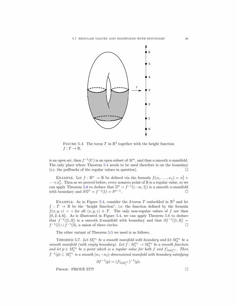
5.7. REGULAR VALUES AND MANIFOLDS WITH BOUNDARY 39

Figure 5.4. The torus T in R3 together with the height functionf : T → R.

is an open set, then f−1(U) is an open subset ofMn, and thus a smooth n-manifold.The only place where Theorem 5.4 needs to be used therefore is on the boundary(i.e. the pullbacks of the regular values in question). □

Example. Let f : Rn → R be defined via the formula f(x1, . . . , xn) = x21 +· · ·+x2n. Then as we proved before, every nonzero point of R is a regular value, so wecan apply Theorem 5.6 to deduce that Dn = f−1((−∞, 1]) is a smooth n-manifoldwith boundary and ∂ Dn = f−1(1) = Sn−1. □

Example. As in Figure 5.4, consider the 2-torus T embedded in R3 and letf : T → R be the “height function”, i.e. the function defined by the formulaf(x, y, z) = z for all (x, y, z) ∈ T . The only non-regular values of f are then{0, 2, 4, 6}. As is illustrated in Figure 5.4, we can apply Theorem 5.6 to deducethat f−1([1, 3]) is a smooth 2-manifold with boundary and that ∂f−1([1, 3]) =f−1(1) ∪ f−1(3), a union of three circles. □

The other variant of Theorem 5.5 we need is as follows.

Theorem 5.7. Let Mn11 be a smooth manifold with boundary and let Mn2

2 be asmooth manifold (with empty boundary). Let f :Mn1

1 →Mn22 be a smooth function

and let p ∈ Mn22 be a point which is a regular value for both f and f |∂Mn1

1. Then

f−1(p) ⊂Mn11 is a smooth (n1−n2)-dimensional manifold with boundary satisfying

∂f−1(p) = (f |∂Mn11

)−1(p).

Proof. PROVE IT!!! □


5.8. Sard’s theorem

The following important theorem says that every smooth map has many regularvalues.

Theorem 5.8 (Sard’s theorem). Let f : M1 → M2 be a smooth map betweensmooth manifolds with boundary. Assume that M1 is compact. Then the set ofregular values of f is open and dense in M2.


5.9. Embedding manifolds in Euclidean space II

We now strengthen Theorem 5.1.

Theorem 5.9. If Mn is a compact smooth n-manifold with boundary, thenthere exist an embedding f :Mn → R2n+1.


5.10. Application: the fundamental theorem of algebra

We now show how to apply the ideas we have introduced to prove the funda-mental theorem of algebra, which can be stated as follows.

Theorem 5.10 (Fundamental theorem of algebra). Let f(z) be a nonconstantpolynomial whose coefficients are complex numbers. Then there exists some z0 ∈ Csuch that f(z0) = 0.

For the proof of Theorem 5.10, we will need the following.

Lemma 5.11. Let Mn be a compact connected manifold whose dimension n isat least 2 and let f : Mn → Mn be a smooth map which is a submersion except atpossibly finitely many points. Then for all regular values p1 ∈ Mn and p2 ∈ Mn,we have |f−1(p1)| = |f−1(p2)|.

Proof. Let R be the set of regular values of f . Define ψ : R → Z ∪ {∞} viathe formula

ψ(p) = |f−1(p)| (p ∈ R).

We must prove that ψ is constant. Our assumptions imply that all but finitely manypoints of Mn are regular values for f . Since n ≥ 2, this implies that R is open andconnected, so it is enough to prove that the function ψ is locally constant. In otherwords, fixing some p ∈ R we must prove that there exists some neighborhood of pin R such that ψ restricted to that neighborhood is constant.

By Theorem 5.5, the set f−1(p) is a 0-dimensional submanifold of Mn. SinceMn is compact, this implies that f−1(p) is a finite set; enumerate it as {q1, . . . , qk}.The function f is a submersion at each qi, so by Theorem 5.2 (the Implicit FunctionTheorem) the function f is a local diffeomorphism at qi, i.e. there exists neighbor-hoods Ui of qi and Wi of p such that f restricts to a diffeomorphism from Ui toWi. Shrinking the Ui if necessary, we can assume that they are all disjoint. Set

W =W1 ∩W2 ∩ · · · ∩Wk

and

U ′i = U1 ∩ f−1(Wi).

5.11. APPLICATION: THE BROUWER FIXED POINT THEOREM 41

By construction, W is a neighborhood of p and f |U ′iis a diffeomorphism between

U ′i and W . What we would really like would be for f−1(W ) to equal U ′

1 ∪ · · · ∪U ′k;

however, this might not hold. To fix this, let C be the closure of the set

f−1(W ) \ (U ′1 ∪ · · · ∪ U ′

k).

The set C is a closed (hence compact) subset of Mn that does not contain any qi.The image f(C) is thus a compact subset of Mn that does not contain p, so we canfind an open neighborhood W ′ of p such that W ′ ⊂ W and W ′ ∩ f(C) = ∅. SetU ′′i = f−1(W ′)∩U ′

i . The restriction f |U ′′iis thus a diffeomorphism from U ′′

i to W ′

and f−1(W ′) = U ′′1 ∪ · · · ∪ U ′′

k .We are now done: for p′ ∈W ′, the preimage f−1(p′) contains exactly one point

from each U ′′i and nothing else. In other words, ψ|W ′ = k, as desired. □

Proof of Theorem 5.10. We will use the second smooth atlas for S2 thatwas discussed in §2.2, which we now recall. Let U1 = S2 \ {(0, 0, 1)} and U−1 =S2 \ {(0, 0,−1)}. Identifying R2 with the subspace of R3 consisting of points whoselast coordinate is 0, define a function ϕ1 : U1 → R2 by letting ϕ1(p) be the uniqueintersection point of the line joining p ∈ U1 ⊂ S2 ⊂ R3 and (0, 0, 1) with the planeR2. It is clear that ϕ1 is a homeomorphism. Similarly, define ϕ−1 : U−1 → R2 byletting ϕ−1(p) be the unique intersection point of the line joining p ∈ U−1 ⊂ S2 ⊂R3 and (0, 0,−1) with the plane R2. Again, ϕ−1 is a homeomorphism. Then theset {ϕ1 : U1 → Rn, ϕ−1 : U−1 → Rn} is a smooth atlas for S2.

Identify C with R2 in the usual way, so we can plug points of R2 into thepolynomial f . Also, for simplicity set ∞ = (0, 0, 1) ∈ S2. Define a functionF : S2 → S2 via the formula

F (x) =

{∞ if x = ∞,

ϕ−11 (f(ϕ1(x))) if x ∈ S2 \ {∞}.

(x ∈ S2).

It is easy to see that F is a smooth map and that F takes S2 \ {∞} to itself(the omitted calculation showing that F is smooth at ∞ uses the fact that f isnonconstant; if f were constant, then F might not even be continuous at ∞). Toprove the fundamental theorem of algebra, it is enough to prove that F is surjective.An easy calculation shows that the only points of S2 where F is not a submersionare

• ϕ−11 (z0), where z0 is a root of the derivative f ′(z), and

• possibly ∞.Since f ′(z) is a polynomial that is not identically 0, it has finitely many roots. Wededuce that F is a submersion except at finitely many points. Letting R ⊂ S2

be the set of regular values of F , Lemma 5.11 therefore implies that the functionΨ : R → Z defined via the formula Ψ−1(p) = |F−1(p)| is constant. Clearly Ψis not identically 0, so this implies that the image of F contains all points of R.Since F definitely contains all points of S2 \ R, we deduce that F is surjective, asdesired. □

5.11. Application: the Brouwer fixed point theorem

We now apply the ideas we have introduced to prove the following theorem. LetDn denote the closed unit disc {(x1, . . . , xn) ∈ Rn | x21 + · · ·+ x2n ≤ 1}, so ∂ Dn =Sn ⊂ Dn.


Theorem 5.12 (Brouwer Fixed Point Theorem). Let f : Dn → Dn be a con-tinuous function. Then there exists some point x ∈ Dn such that f(x) = x.

Remark. To illustrate what is going on here, consider the case n = 1, soDn = [−1, 1] ⊂ R. The theorem asserts that if f : [−1, 1] → [−1, 1] is a continuousfunction, then there exists some point x ∈ [−1, 1] such that f(x) = x. Anotherway of saying this is that the theorem is asserting that the function g : [−1, 1] → Rdefined via the formula g(x) = f(x) − x has a zero. Since g(−1) = f(−1) + 1 ≥ 0and g(1) = f(1)−1 ≤ 0, this is an immediate consequence of the intermediate valuetheorem. □

Proof of Theorem 5.12. We will do this in several steps.

Step 1. There does not exist a smooth function f : Dn → ∂ Dn such thatf |∂ Dn = id.

Assume that such a function exists. Using Theorem 5.8 (Sard’s Theorem),there exists a regular value p ∈ ∂ Dn for f . Since f |∂ Dn = id, the point p is also aregular value for f |∂ Dn . We can therefore apply Theorem 5.7 to deduce that f−1(p)is a smooth 1-manifold with boundary embedded in Dn such that

∂f−1(p) = (f |∂ Dn)−1(p) = {p}.

Recall that every connected compact 1-manifold with boundary is diffeomorphic toeither S1 or [0, 1] (this will be proven in Theorem 11.1 below). But this impliesthat that any compact 1-manifold with boundary (connected or not) has a boundaryconsisting of an even number of points, so this is a contradiction.

Step 2. Let f : Dn → Dn be a smooth function. Then there exists some pointx ∈ Dn such that f(x) = x.

Assume that f(x) = x for all x ∈ Dn. Define a function g : Dn → ∂ Dn asfollows. For x ∈ Dn, let ℓx be the ray starting at x and passing through f(x). Thisis well-defined since f(x) = x. The ray ℓx intersects ∂ Dn at a unique point; letg(x) be this point of intersection. Writing out equations for ℓx, it is clear that thefunction g is smooth. Moreover, by definition we have g|∂ Dn = id. This contradictsStep 1.

Step 3. Let f : Dn → Dn be a continuous function. Then there exists somepoint x ∈ Dn such that f(x) = x.

We will reduce this to Step 2 by approximating f by a smooth function. Assumethat f(x) = x for all x ∈ Dn. Set

ϵ = inf{∥f(x)− x∥ | x ∈ Dn}.

Since Dn is compact, this infimum is realized and ϵ > 0. Use Lemma 2.8 to find asmooth function g : Dn → Rn such that ∥g(x) − f(x)∥ < ϵ/3 for all x ∈ Dn. Theimage of g need not lie in Dn; however, we have ∥g(x)∥ ≤ ∥f(x)∥ + ϵ/3 ≤ 1 + ϵ/3for all x ∈ Dn. Defining h : Dn → Rn via the formula

h(x) =g(x)

1 + ϵ/3,

we deduce that h(Dn) ⊂ Dn. To get a contradiction to Step 2, we will provethat h has no fixed points. For all x ∈ Dn, it follows from the definitions that

5.11. APPLICATION: THE BROUWER FIXED POINT THEOREM 43

∥h(x)− g(x)∥ ≤ ϵ/3. The triangle inequality then implies that

∥h(x)− x∥ ≥ ∥f(x)− x∥ − ∥f(x)− g(x)∥ − ∥g(x)− h(x)∥ ≥ ϵ− ϵ/3− ϵ/3 = ϵ/3.

Since ϵ > 0, this implies that h(x) = x. This contradicts Step 2, and we aredone. □

CHAPTER 6

Tubular neighborhoods

In this chapter, we discuss tubular neighborhoods together with some of theirapplications. For simplicity, we will restrict ourselves to tubular neighborhoods ofsubmanifolds of Euclidean space.

6.1. Normal bundles

We first must discuss normal bundles. To define these, we will use the vectorbundle operations that we discussed in §3.8.

Definition. Let Mn11 and Mn2

2 be smooth manifolds and let f :Mn11 →Mn2

2

be an embedding. There is a map g : TMn11 → f∗(TMn1

2 ) of vector bundles overMn1

1 which since f is an embedding restricts to an injection (TMn11 )p → f∗(TMn1

2 )pfor each p ∈Mn1

1 . The normal bundle to f , denoted Nf , is the cokernel of g. Thisis an (n2 − n1)-dimensional vector bundle over Mn1

1 . □

The following special case of this will be particularly important.

Definition. Let Mn be a smooth submanifold of Rm. We will denote byNRm/Mn the normal bundle to the inclusion map Mn ↪→ Rm. □

The normal bundle to a smooth submanifold of Rm can be expressed in aparticuarly simple form. Recall that if Mn is a smooth submanifold of Rm, thenTpM

n is canonically identified with an n-dimensional subspace of TpRm = Rm forall p ∈Mn.

Definition. If Mn is a smooth submanifold of Rm and p ∈ Mn, then denoteby Np,Rm/Mn the orthogonal complement to TpM

n in TpRm = Rm. □

Lemma 6.1. Let Mn be a smooth submanifold of Rm. Then

NRm/Mn ∼= {(p, v) ∈ TRm | p ∈Mn and v ∈ Np,Rm/Mn}.

Proof. This is an exercise. □

Example. For Sn ⊂ Rn+1 and p ∈ Sn, recall that TpSn consists of all vectors

in TpRn+1 = Rn+1 that are orthgonal to the line from 0 to p. This implies that

NRn+1/Sn = {(p, tp) | p ∈ Sn, t ∈ R} ∼= Sn × R. □

Since NRm/Mn is an (m−n)-dimensional vector bundle overMn, it is a smoothm-dimensional manifold. The following lemma identifies its tangent space. In it,we make use of the fact that

T (TRn) = T (Rn × Rn) = (Rn × Rn)× (Rn × Rn).

45

46 6. TUBULAR NEIGHBORHOODS

Figure 6.1. A tubular neighborhood of a loop S1 embedded in R2

Lemma 6.2. LetMn be a smooth submanifold of Rm and let (p, v) ∈ NRm/Mn ⊂TRm = Rm × Rm. Then the tangent space T(p,v)NRm/Mn consists of all points(w, w′) ∈ T(p,v)(Rm × Rm) = Rm × Rm such that w ∈ TpM

n ⊂ Rm and w′ ∈Np,Rm/Mn ⊂ Rm.

Proof. This is another exercise. □

6.2. The tubular neighborhood theorem

We now come to the tubular neighborhood theorem. This requires a definition.In it, we make use of the identification described in Lemma 6.1

Definition. Let Mn be a smooth submanifold of Rm. For ϵ > 0, defineN ϵ

Rm/Mn to be the subspace of NRm/Mn consisting of points (p, v) such that p ∈Mn

and v ∈ Np,Rm/Mn ⊂ Rm and ∥v∥ < ϵ. □Theorem 6.3 (Tubular Neighborhood Theorem). LetMn be a smooth compact

submanifold of Rm. Define n : NRm/Mn → Rm to be the map taking (p, v) to p+ v.Then there exists some ϵ such that the restriction of n to N ϵ

Rm/Mn is an embedding.

The image of the restriction of n : NRm/Mn → Rm to N ϵRm/Mn will be called an

ϵ-tubular neighborhood of Mn. To illustrate why it is called this, see Figure 6.1.

Proof of Theorem 6.3. For ϵ > 0 and a set U ⊂ Mn, let N ϵRm/Mn(U)

denote the subspace of N ϵRm/Mn consisting of points (p, v) such that p ∈ U . The

proof will have two steps.

Step 1. There exists an open cover {Ui}ki=1 of Mn and an ϵ > 0 such that nrestricts to an embedding from N ϵ

Rm/Mn(Ui) into Rm for all 1 ≤ i ≤ k.

Since Mn is compact, it is enough to prove that the map n is a local diffeomor-phism at each point (p, 0) ∈ NRm/Mn . By Theorem 5.2 (the Implicit Function The-orem), this is equivalent to showing that D(p,0) n : T(p,0)NRm/Mn → T(p,0)Rm = Rmis an isomorphism. Lemma 6.2 says that T(p,0)NRm/Mn consists of all point (w, w′) ∈T(p,0)(Rm×Rm) = Rm×Rm such that w ∈ TpM

n ⊂ Rm and w′ ∈ Np,Rm/Mn ⊂ Rm.Under this identification, the derivative D(p,0) n takes (w, w′) to w + w′. Since Rmis the orthogonal direct sum of TpM

n and Np,Rm/Mn , it follows that D(p,0) n is anisomorphism, as desired.

6.3. APPROXIMATING CONTINUOUS FUNCTIONS BY SMOOTH ONES, II 47

Step 2. There exists some 0 < ϵ′ < ϵ such that the restriction of n to N ϵ′

Rm/Mn

is an embedding.

Set ϵ′′ = ϵ/2 and define N≤ϵ′Rm/Mn to be the subspace of NRm/Mn consisting of

points (p, v) such that p ∈ Mn and v ∈ Np,Rm/Mn ⊂ Rm and ∥v∥ ≤ ϵ′. Define

N≤ϵ′Rm/Mn(Ui) in the obvious way. Since Mn is compact, it follows that N≤ϵ′

Rm/Mn is

compact. Let X = N≤ϵ′Rm/Mn × N≤ϵ′

Rm/Mn and Y = {(x, y) ∈ X | n(x) = n(y)} and

∆ = {(x, y) ∈ X | x = y}, so both Y and ∆ are closed (hence compact) and ∆ ⊂ Y .Define Z = Y \∆. We claim that Z is compact. Indeed, define

W =k∪i=1

N≤ϵ′Rm/Mn(Ui)×N≤ϵ′

Rm/Mn(Ui) ⊂ X.

The setW is open and by Step 1 we haveW ∩Y = ∆. This implies that Z = Y \W ,so Z is compact, as claimed.

Define

A = {((p, v), (p′, v′)) ∈ X | v = v′ = 0} ∼=Mn ×Mn,

so A is compact. Since n takes {(p, v) ∈ N≤ϵ′Rm/Mn | v = 0} diffeomorphically onto

Mn, it follows that Z ∩A = ∅. Since both Z and A are compact, this implies thatwe can choose 0 < ϵ′ < ϵ′′ such that for all ((p, v), (p′, v′)) ∈ Z we have ∥v∥ ≥ ϵ′

and ∥v′∥ ≥ ϵ′. Unwinding the definitions, this implies that the restriction of n

to N ϵ′

Rm/Mn is injective. Since Step 1 implies that the restriction of n to N ϵ′

Rm/Mn

is a local diffeomorphism, we conclude that the restriction of n to N ϵ′

Rm/Mn is an

embedding, as desired. □

The following corollary to Theorem 6.3 will be frequently used.

Corollary 6.4. Let Mn be a smooth compact submanifold of Rm. Then forall ϵ > 0, there exists some open set Uϵ ⊂ Rm containingMn and a smooth functionπ : Uϵ →Mn with the following properties.

• π(p) = p for all p ∈Mn.• ∥π(p)− p∥ < ϵ for all p ∈ Uϵ.

Proof. Decreasing ϵ if necessary, we can apply Theorem 6.3 to construct an ϵ-tubular neighborhood Uϵ of M

n. We have Uϵ ∼= N ϵRm/Mn ; under this identification,

the desired function π : Uϵ → Mn is function that takes (p, v) ∈ N ϵRm/Mn to p.

This clearly satisfies the claimed properties. □

6.3. Approximating continuous functions by smooth ones, II

Recall that in Theorem 2.7 we proved that if M is a smooth manifold andf :M → Rm is a continuous function, the f can be approximated arbitrarly well bysmooth functions. As a first application of the tubular neighborhood, we now showhow to approximate continuous functions between arbitrary compact manifolds bysmooth ones.

Theorem 6.5. LetM1 be a smooth manifold with boundary, letM2 be a smoothcompact manifold, and let f : M1 → M2 be a continuous function. Let dM2(·, ·)be a metric (in the sense of metric spaces) on M2 that induces the topology on

48 6. TUBULAR NEIGHBORHOODS

M2. Then for all ϵ > 0 there exists a smooth function g : M1 → M2 such thatdM2(f(x), g(x)) < ϵ for all x ∈M1.

Proof. Using Theorem 5.1, we can embed M2 into Rm for some m≫ 0. Thesubspace topology on M2 induced by Rm is the same as the topology induced bythe metric dM2(·, ·), so we can find some ϵ′ > 0 such that if ∥y1 − y2∥ < ϵ′ for somey1, y2 ∈M2, then dM2(y1, y2) < ϵ. Shrinking ϵ′ if necessary, we can apply Corollary6.4 to construct an open neighborhood Uϵ′/2 of M2 together with a function π :Uϵ′/2 → M2 such that π(p) = p for all p ∈ M2 and ∥π(p) − p∥ < ϵ′/2 for allp ∈ Uϵ′/2. Applying Theorem 2.7 to our continuous function f : M1 → M2 ⊂ Rm,we can find a smooth function g1 : M1 → Rm such that ∥f(x) − g1(x)∥ < ϵ′/2 forall x ∈ M1. The image of g1 will no longer lie in the subspace M2 of Rm, but itwill lie in Uϵ′/2. Define g = π ◦ g1, so g is a smooth function from M1 to M2. Forx ∈M1, we then have

∥f(x)− g(x)∥ ≤ ∥f(x)− g1(x)∥+ ∥g1(x) + π(g1(x))∥ < ϵ′/2 + ϵ′/2 = ϵ′,

and hence dM2(f(x), g(x)) < ϵ, as desired. □The following “relative” version of Theorem 6.5 will also be useful.

Theorem 6.6. LetM1 be a smooth manifold with boundary, letM2 be a smoothcompact manifold, and let f :M1 →M2 be a continuous function. Also, let U ⊂M1

be an open set such that f |U is smooth and let C ⊂M1 be a closed set with C ⊂ U .Let dM2(·, ·) be a metric (in the sense of metric spaces) on M2 that induces thetopology on M2. Then for all ϵ > 0, there exists a smooth function g : M1 → M2

such that dM2(f(x), g(x)) < ϵ for all x ∈M1 and such that g|C = f |C .

Proof. Simply replace the invocation of Theorem 2.7 in the proof of Theorem6.5 with Theorem 2.9. □

CHAPTER 7

The degree of a map

7.1. Homotopies and smooth homotopies

We begin with the following topological relationship between functions.

Definition. Let f0, f1 : X → Y be continuous functions between topologicalspaces. We say that f0 and f1 are homotopic if there exists a continuous functionF : X × I → Y such that F (x, 0) = f0(x) and F (x, 1) = f1(x) for all x ∈ X. Thefunction F will be called a homotopy. □

In other words, the function f0 can be “deformed” to the function f1. Here isone easy example of this.

Example. Let X be a topological space and let f0, f1 : X → Rn be continuousfunctions. Then f0 and f1 are homotopic via the homotopy F : X×I → Rn definedby the formula

F (x, t) = (1− t)f0(x) + tf1(x) (x ∈ X).

In other words, F moves the point f0(x) to the point f1(x) along the straight lineconnecting these two points. □

Lemma 7.1. For topological spaces X and Y , the relation of homotopy betweencontinuous functions from X to Y is an equivalence relation.

Proof. Trivial. □If M1 and M2 are smooth manifolds, then we have two seemingly different

equivalence classes of functions from M1 to M2.• Continuous functions up to homotopy.• Smooth functions up to smooth homotopy, that is, homotopies F : M1 ×I →M2 that are themselves smooth.

The two main theorems in this section show that these are really the same thing.The first is as follows.

Theorem 7.2. Let f : M1 → M2 be a continuous function between smoothcompact manifolds. Then f is homotopic to a smooth function g :M1 →M2.

Proof. Using Theorem 5.1, we can embed M2 into Rm for some m ≫ 0.Using Corollary 6.4, we can find an open neighborhood U of M2 in Rm and asmooth function π : U → M2 such that π(p) = p for all p ∈ M2 (the constant ϵ inthat corollary does not matter for this proof). We can now pick δ > 0 small enoughsuch that if p1, p2 ∈M2 satisfy ∥p1−p2∥ < δ, then the straight line segment from p1to p2 lies in U . Now use Theorem 6.5 to construct a smooth function g :M1 →M2

such that ∥f(p) − g(p)∥ < δ for all p ∈ M1. We claim that f is homotopic to g.Indeed, the function F :M1 × I →M2 defined via the formula

F (p, t) = π((1− t)f(p) + tg(p)) (p ∈M1, t ∈ I)

49

50 7. THE DEGREE OF A MAP

is a homotopy from f to g. This is well-defined since (1 − t)f(p) + tg(p) ∈ U(the domain of π) for all t ∈ I and p ∈ I, which is a consequence of the fact that∥f(p)− g(p)∥ < δ. □

The second is as follows.

Theorem 7.3. Let f0 : M1 → M2 and f1 : M1 → M2 be homotopic smoothfunctions between smooth compact manifolds. Then there exists a smooth homotopybetween f0 and f1.

Proof. Let F : M1 × I → M2 be a continuous homotopy between f0 and f1.Modifying F , we can assume that F (p, t) = f0(p) for 0 ≤ t ≤ 1/3 and F (p, t) =f1(p) for 2/3 ≤ t ≤ 1. Thus F is smooth on the open set M × ([0, 1/3) ∪ (2/3, 1]).Applying Theorem 6.6, we can find a smooth function G : M1 × I → M2 suchthat G(p, 0) = F (p, 0) = f0(p) and G(p, 1) = F (p, 1) = f1(p) for all p ∈ M1 (wecould also ensure that ∥G(p, t)− F (p, t)∥ < ϵ for all (p, t) ∈M1 × I, but this is notnecessary). The function G is the desired smooth homotopy. □

7.2. Homotopies and regular values

This technical section will discuss the relationship between homotopy classes offunctions and regular values. Our two results augment Theorems 7.2 and 7.3 fromthe previous section.

Lemma 7.4. Let f : M1 → M2 be a continuous function between smoothcompact manifolds and let p ∈ M2. Then f is homotopic to a smooth functiong :M1 →M2 such that p is a regular value of g.

Proof. By Theorem 7.2, we can assume that f is itself smooth. Using Theo-rem 5.8 (Sard’s Theorem), we can find a regular value q ∈ M2 of f . Theorem 4.7implies that we can find a flow ht :M2 →M2 of a vector field such that h1(q) = p.Define g = h1 ◦ f . Since h1 is a diffeomorphism, the point p is a regular value of g.Moreover, f is homotopic to g via the homotopy F :M1 × I →M2 defined via theformula

F (x, t) = ht(f(x)) (x ∈M1, t ∈ I);

here we are using the fact that h0 = id, which follows from the definition of aflow. □

Lemma 7.5. Let f0 : M1 → M2 and f1 : M1 → M2 be homotopic smoothfunctions between smooth compact manifolds and let p ∈ M2 be a point which is aregular value of both f0 and f1. Then there exists a smooth homotopy F :M1×I →M2 such that p is a regular value of both f0 and f1.


7.3. The degree modulo 2

We now come to the first and most primitive notion of the degree of a smoothmap between compact manifolds of the same dimension.

Definition. Let Mn1 and Mn

2 be smooth compact manifolds of the same di-mension and let f : Mn

1 → Mn2 be a continuous function. The mod-2 degree of f ,

denoted deg2(f), is the element of Z/2 defined as follows.

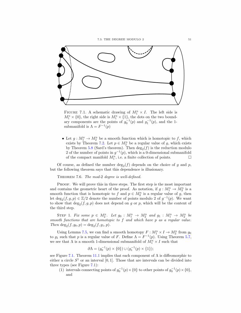
7.3. THE DEGREE MODULO 2 51

Figure 7.1. A schematic drawing of Mn1 × I. The left side is

Mn1 × {0}, the right side is Mn

1 × {1}, the dots on the two bound-ary components are the points of g−1

0 (p) and g−11 (p), and the 1-

submanifold is Λ = F−1(p)

• Let g : Mn1 → Mn

2 be a smooth function which is homotopic to f , whichexists by Theorem 7.2. Let p ∈ Mn

2 be a regular value of g, which existsby Theorem 5.8 (Sard’s theorem). Then deg2(f) is the reduction modulo2 of the number of points in g−1(p), which is a 0-dimensional submanifoldof the compact manifold Mn

1 , i.e. a finite collection of points. □

Of course, as defined the number deg2(f) depends on the choice of g and p,but the following theorem says that this dependence is illusionary.

Theorem 7.6. The mod-2 degree is well-defined.

Proof. We will prove this in three steps. The first step is the most importantand contains the geometric heart of the proof. As notation, if g : Mn

1 → Mn2 is a

smooth function that is homotopic to f and p ∈ Mn2 is a regular value of g, then

let deg2(f, g, p) ∈ Z/2 denote the number of points modulo 2 of g−1(p). We wantto show that deg2(f, g, p) does not depend on g or p, which will be the content ofthe third step.

Step 1. Fix some p ∈ Mn2 . Let g0 : Mn

1 → Mn2 and g1 : Mn

1 → Mn2 be

smooth functions that are homotopic to f and which have p as a regular value.Then deg2(f, g0, p) = deg2(f, g1, p).

Using Lemma 7.5, we can find a smooth homotopy F :Mn1 × I →Mn

2 from g0to g1 such that p is a regular value of F . Define Λ = F−1(p). Using Theorem 5.7,we see that Λ is a smooth 1-dimensional submanifold of Mn

1 × I such that

∂Λ = (g−10 (p)× {0}) ∪ (g−1

1 (p)× {1});

see Figure 7.1. Theorem 11.1 implies that each component of Λ is diffeomorphic toeither a circle S1 or an interval [0, 1]. Those that are intervals can be divided intothree types (see Figure 7.1):

(1) intervals connecting points of g−10 (p)×{0} to other points of g−1

0 (p)×{0},and


(2) intervals connecting points of g−11 (p)×{1} to other points of g−1

1 (p)×{1},and

(3) intervals connecting points of g−10 (p)× {0} to points of g−1

1 (p)× {1}.Let k0 (resp. k1) be the number of points of g−1

0 (p)×{0} (resp. g−11 (p)×{1}) that

occur as endpoints of intervals of the first (resp. second) type. Both k0 and k1are even. Next, let ℓ0 (resp. ℓ1) be the number of points of g−1

0 (p) × {0} (resp.g−11 (p) × {1}) that occur as endpoints of intervals of the third type. We clearlyhave ℓ0 = ℓ1. We have

|g−10 (p)| = k0 + ℓ0 and |g−1

1 (p)| = k1 + ℓ1.

Since the ki are even and the ℓi are equal, we deduce that reductions modulo 2 of|g−1

0 (p)| and |g−11 (p)| are the same, as desired.

Step 2. Let g : Mn1 → Mn

2 be a smooth function that is homotopic to f andlet p, q ∈M2 be regular values of g. Then deg2(f, g, p) = deg2(f, g, q).

Using Theorem 4.7, we can find a flow ht : M2 → M2 of a smooth vector fieldsuch that ht(p) = q. Define g1 = h1 ◦ g. Since h1 is a diffeomorphism of M2, thepoint q is a regular value of g1. In fact, we have g−1(p) = g−1

1 (q). Moreover, g1is homotopic to g (and hence f) via the homotopy F : M1 × I → M2 defined viaF (x, t) = h1−t(g(x)) for (x, t) ∈ M1 × I. This ends at g since h0 = id. We thushave that

deg2(f, g, p) = deg2(f, g1, q) = deg2(f, g, q),

where the first equality follows from the fact that g−1(p) = g−11 (q) and the second

from Step 1.

Step 3. Let g0 : Mn1 → Mn

2 and g1 : Mn1 → Mn

2 be smooth functions that arehomotopic to f . Let p0 ∈Mn

2 be a regular value of g0 and let p1 ∈Mn2 be a regular

value of g1. Then deg2(f, g0, p0) = deg2(f, g1, p1).

By Theorem 5.8 (Sard’s theorem), the regular values of g0 are open and densein Mn

2 , and similarly for g1. We can thus find some point q ∈Mn2 that is a regular

value of both g0 and g1. Applying Steps 1 and 2, we see that

deg2(f, g0, p0) = deg2(f, g0, q) = deg2(f, g1, q) = deg2(f, g1, p1),

as desired. □

7.4. Simple applications of the mod-2 degree

One simple application of the mod-2 degree is as follows.

Theorem 7.7. Let Mn be a smooth compact manifold and let f : Mn → Mn

be a diffeomorphism. Then f is not homotopic to a constant map.

Proof. Since every point ofMn is a regular value of f and has a single preim-age, we see that deg2(f) = 1. However, if g : Mn → Mn is a constant map, thenthe regular values of g are exactly those points not in its image, so deg2(g) = 0.Since deg2(f) = deg2(g), we see that f and g are not constant. □

This gives an alternate proof of the following result, which we recall is the keytopological fact used to prove the Brouwer fixed point theorem (Theorem 5.12).

Lemma 7.8. There does not exist a smooth map f : Dn → Sn such that f(p) = pfor all p ∈ Sn.

7.5. ORIENTATIONS ON VECTOR SPACES 53

Proof. Assume that such an f exists. The function F : Sn × I → Sn definedvia the formula

F (p, t) = f((1− t)p) (p ∈ Sn, t ∈ I)

is a homotopy from the identity map on Sn to the constant map with image f(0),which constradicts Theorem 7.7. □

7.5. Orientations on vector spaces

Our next goal will be to refine the mod-2 degree to a degree that takes integervalues. To do this, we will have to introduce orientations on our manifolds. Webegin in this section by discussing orientations on vector spaces.

Definition. Let V be an n-dimensional real vector space with n ≥ 1. Anorientation on V is an equivalence class of ordered basis (v1, . . . , vn) for V underthe following equivalence relation:

• If b = (v1, . . . , vn) and b′ = (v′1, . . . , v′n) are ordered bases for V , then

b ∼ b′ if det(aij) > 0, where (aij) is the n × n change of basis matrixdefined via the identities

v′i =n∑j=1

aij vj (1 ≤ i ≤ n).

If V is equipped with a fixed orientation, then we will call V an oriented vector spaceand any ordered basis representing that orientation an oriented basis for V . □

The first basic property of orientations is as follows.

Lemma 7.9. Let V be an n-dimensional real vector space with n ≥ 1. Then Vhas exactly two orientations.

Proof. Let b = (v1, . . . , vn) and b′ = (v′1, . . . , v′n) be two ordered bases for

V . Since multiplying a column of a matrix by −1 has the effect of multiplying itsdeterminant by −1, it follows that b represents the same orientation as either b′ of(−v′1, v′2, . . . , v′n). □

This lemma implies that the following definition makes sense.

Definition. Let V be an n-dimensional real vector space and let b be anorientation of V . Then −b will denote the other orientation. □

The following lemma will be very useful.

Lemma 7.10. Let f : V → W be a surjective map between finite-dimensionalreal vector spaces of positive dimension. Set U = ker(f) and assume that U haspositive dimension. Assume that two out of the three vector spaces U and V andW are equipped with an orientation. There is then a unique way to choose anorientation for the third such that the following holds.

• Let w1, . . . , wk ∈ V be vectors such that (f(w1), . . . , f(wk)) is an orientedbasis for W . Also, let (u1, . . . , uℓ) be an oriented basis for U . Then(w1, . . . , wk, u1, . . . , vℓ) is an oriented basis for V .

Proof. Homework! I’ll insert this proof after the homework is due. □


7.6. Orientation on manifolds

We now define orientations on smooth manifolds. Informally, an orientationon a smooth manifold is a choice of orientation on each tangent space that “varysmoothly”. Since there are two orientations on a vector space, the set of possi-ble orientations on a particular tangent space is a discrete set and the notion of“vary smoothly” should really mean “is locally constant”. We formalize this in thefollowing definition.

Definition. An orientation on a smooth manifold with boundary Mn is achoice of orientation bp of TpM

n for all p ∈Mn that satisfy the following continuitycondition:

• Let ϕ : U → V be any chart. For any p ∈ U , let bp be the orientation onTϕ(p)V = Rn induced by bp under the canonical identification of TpM

n

with Tϕ(p)V . Then we require that bp = bp′ for all p, p′ ∈ U .

A manifold with boundary Mn is orientable it there exists an orientation on it.An oriented manifold with boundary is a smooth manifold with boundary that isequipped with an orientation. □

The easiest example is as follows.

Example. Let V be an open subset of Rn. Equip each tangent space TpV = Rnwith the orientation corresponding to the standard basis of Rn. This gives anorientation on V . □

To give more examples, we need the following lemma.

Lemma 7.11. Let f : M1 → M2 be a smooth map between a smooth manifoldwith boundary M1 and a smooth oriented manifold M2 and let p ∈M2 be a regularvalue of both f and f |∂M1 . Then f−1(p) is orientable.

Proof. Set X = f−1(p). Recall that Theorem 5.7 says that X is a smoothmanifold with boundary and that ∂X = (f |∂M1)

−1(p). For each q ∈ X, we havethat

TqX = ker(Dqf : TqM1 → TpM2).

Since p is a regular value, the map Dqf is surjective. Using Lemma 7.10, our givenorientations on TpM2 and TqM1 induce a canonical orientation on TqX. It is easyto see that these orientations on the tangent spaces of X vary smoothly, so thisgives us an orientation on X. □

Example. Let f : Rn+1 → R be the function f(x1, . . . , xn+1) =∑n+1i=1 x

2i . We

know that 1 is a regular value of f and that Sn = f−1(1). Since both Rn+1 and Rare orientable, we deduce from Lemma 7.11 that Sn is orientable. □

Our next goal is to show how to orient the boundary of an orientable manifoldwith boundary. This requires the following definition.

Definition. Let Mn be a smooth manifold with boundary, let p ∈ ∂Mn, andlet v ∈ TpM

n. Choose a chart ϕ : U → V with p ∈ U and V ⊂ Hn.• We say that v is tangent to the boundary if the last coordinate of theelement of Tϕ(p)V = Rn corresponding to v is zero. Equivalently, v lies inTp(∂M

n) ⊂ TpMn.

• We say that v is inward facing if the last coordinate of the element ofTϕ(p)V = Rn corresponding to v is positive.

7.7. THE INTEGRAL DEGREE 55

• We say that v is outward facing if the last coordinate of the element ofTϕ(p)V = Rn corresponding to v is negative.

It is easy to see that these notions are well-defined. □Lemma 7.12. Let Mn be a smooth oriented manifold with boundary. Then

there exists a unique orientation on ∂Mn with the following property:• Let (v1, . . . , vn−1) be an oriented basis for Tp(∂M

n) ⊂ TpMn and let

vn ∈ TpMn be an inward facing vector. Then (v1, . . . , vn) is an oriented

basis for TpMn.

Proof. That this condition picks out a unique orientation on each Tp(∂Mn)

follows from Lemma 7.10. It is easy to see that it varys smoothly, and thus givesan orientation on ∂Mn. □

We will call the orientation given by Lemma 7.12 the inward facing orientationon ∂Mn. In a similar way, we can define the outward facing orientation on ∂Mn.

Example. Since Dn ⊂ Rn is orientable, Lemma 7.12 gives another proof thatSn = ∂Dn is orientable. □

7.7. The integral degree

We now define the degree of a continuous function between compact orientedn-manifolds. This requires the following preliminary definition.

Definition. Let g : Mn1 → Mn

2 be a smooth map between orientable n-manifolds and let q ∈Mn

1 be such that g is a submersion at q. The derivative mapTqg : TqM

n1 → Tf(q)M

n2 is thus an isomorphism. Define ϵg,q to be +1 if Tqg takes

the given orientation on TqMn1 to the given orientation on Tf(q)M

n2 and to be −1

if it does not. □We then define the degree as follows.

Definition. Let Mn1 and Mn

2 be smooth compact oriented manifolds of thesame dimension and let f : Mn

1 → Mn2 be a continuous function. The degree of f ,

denoted deg(f), is the element of Z defined as follows.• Let g : Mn

1 → Mn2 be a smooth function which is homotopic to f , which

exists by Theorem 7.2. Let p ∈ Mn2 be a regular value of g, which exists

by Theorem 5.8 (Sard’s theorem). Then

deg(f) =∑

q∈f−1(p)

ϵg,q,

which is a finite sum since g−1(p) is a 0-dimensional submanifold of thecompact manifold Mn

1 , i.e. a finite collection of points. □Just like for the mod-2 degree, we must prove that this is well-defined.

Theorem 7.13. The degree is well-defined.

Proof. The proof of this is very similar to the proof of Theorem 7.6, whichproves the analogous fact for the mod-2 degree. As notation, if g :Mn

1 →Mn2 is a

smooth function that is homotopic to f and p ∈ Mn2 is a regular value of g, then

letdeg(f, g, p) =

∑q∈f−1(p)

ϵg,q.


We want to show that deg(f, g, p) does not depend on g or pAgain, there will be three steps.

Step 1. Fix some p ∈ Mn2 . Let g0 : Mn

1 → Mn2 and g1 : Mn

1 → Mn2 be

smooth functions that are homotopic to f and which have p as a regular value.Then deg(f, g0, p) = deg(f, g1, p).

Using Lemma 7.5, we can find a smooth homotopy F :Mn1 × I →Mn

2 from g0to g1 such that p is a regular value of F . Define Λ = F−1(p). Using Theorem 5.7,we see that Λ is a smooth 1-dimensional submanifold of Mn

1 × I such that

∂Λ = (g−10 (p)× {0}) ∪ (g−1

1 (p)× {1});see Figure 7.1.

At this point, we have to be careful with orientations. Observe first that wecan orient Mn

1 × I in such a way that the inward-facing orientation on Mn1 ×{0} ⊂

∂(Mn1 × I) is the given orientation on Mn

1 . However, with this choice of orientationthe given orientation on Mn

1 is the outward-facing orientation on Mn1 × {1} ⊂

∂(Mn1 × I). Now, Lemma 7.11 says that our given orientations on Mn

1 and Mn2

induce a canonical orientation on Λ. An orientation on a 1-dimensional manifold isjust a choice of direction for each component. Chasing through the proof of Lemma7.11, we see that our orientation on Λ satisfies the following property:

• Consider a point q ∈ Λ. We then have that

TqΛ = ker(DqF : Tq(Mn1 × I) → TpM

n2 ).

Let v ∈ TqΛ be a vector such that (v) is an oriented basis for TqΛ. Also, letw1, . . . , wn ∈ Tq(M

n1 × I) be elements such that (DqF (w1), . . . , DqF (wn))

is an oriented basis for TpMn2 . Then (w1, . . . , wn, v) is an oriented basis

for Tq(Mn1 × I).

Theorem 11.1 implies that each component of Λ is diffeomorphic to either a circleS1 or an interval [0, 1]. Those that are intervals can be divided into three types(see Figure 7.1). In our descriptions of these types, we use our given orientation onΛ to speak of an interval having an initial and a terminal point.

(1) Intervals having an initial point q ∈ g−10 (p)×{0} and a terminal point q′ ∈

g−10 (p)×{0}. We claim that ϵg0,q = 1 and ϵg0,q′ = −1. Indeed, let v ∈ TqΛbe a vector such that (v) is an oriented basis for TqΛ. We have q ∈ ∂(Mn

1 ×I) and v is an inward-facing vector. Choose an ordered basis (w1, . . . , wn)for Tq(∂M

n1 × I) ⊂ Tq(M

n1 × I) such that (DqF (w1), . . . , DqF (wn)) is an

oriented basis for TpMn2 . Then by the above discussion of the orientation

on Λ we have that (w1, . . . , wn) is an oriented basis for Tq(Mn2 × {0}),

which implies that ϵg0,q = 1. In a similar way, we see that ϵg0,q′ = −1;the reason for the change in sign is that if v′ ∈ Tq′Λ is such that (v′) isan oriented basis for Tq′Λ, then v

′ is an outward-facing vector.

(2) Intervals having an initial point q ∈ g−11 (p) × {1} and a terminal point

q′ ∈ g−11 (p) × {1}. Just like in the first case, we have ϵg1,q = −1 and

−ϵg1,q′ = 1.

(3) Intervals having an initial point q ∈ g−10 (p) × {0} and a terminal point

q′ ∈ g−11 (p)× {1}. In this case, an argument similar to that above shows

that ϵg0,q = ϵg1,q′ . The key point here is that the relevant orientation onMn

1 ×{0} is the inward-facing orientation but the relevant orientation onMn

1 × {1} is the outward-facing orientation.

7.7. THE INTEGRAL DEGREE 57

Adding all the points up, we see that the positive and negative signs of the pointsappearing at the endpoints of the intervals of the first and second types all cancel,while the intervals of the third type match up points with identical signs. Thisimplies that deg(f, g0, p) = deg(f, g1, p), as desired.

Step 2. Let g : Mn1 → Mn

2 be a smooth function that is homotopic to f andlet p, q ∈M2 be regular values of g. Then deg(f, g, p) = deg(f, g, q).

The proof is identical to that of the analogous step of the proof of Theorem7.6, so we omit it.

Step 3. Let g0 : Mn1 → Mn

2 and g1 : Mn1 → Mn

2 be smooth functions that arehomotopic to f . Let p0 ∈Mn

2 be a regular value of g0 and let p1 ∈Mn2 be a regular

value of g1. Then deg2(f, g0, p0) = deg2(f, g1, p1).

Again, the proof is identical to that of the analogous step of the proof ofTheorem 7.6, so we omit it. □

CHAPTER 8

Foliations and Frobenius’s theorem

59

CHAPTER 9

Lie groups

61

CHAPTER 10

Transversality

63

CHAPTER 11

Morse theory

Theorem 11.1 (Classification of 1-manifolds). Every compact connected 1-manifold with boundary is diffeomorphic to either S1 or [0, 1].

65

CHAPTER 12

Orientations and integral degrees

67

CHAPTER 13

Winding numbers and the Hopf invariant

69

CHAPTER 14

The Poincare-Hopf theorem

Theorem 14.1 (Hairy ball theorem). There does not exist a nonvanishingvector field on an even-dimensional sphere S2n.

71

a geometrically-minded introduction to smooth manifolds · smooth manifolds this chapter de nes...

Documents