chapter 1 smooth manifolds

Chapter 1Smooth Manifolds

This book is about smooth manifolds. In the simplest terms, these are spaces thatlocally look like some Euclidean space Rn, and on which one can do calculus. Themost familiar examples, aside from Euclidean spaces themselves, are smooth planecurves such as circles and parabolas, and smooth surfaces such as spheres, tori,paraboloids, ellipsoids, and hyperboloids. Higher-dimensional examples include theset of points in RnC1 at a constant distance from the origin (an n-sphere) and graphsof smooth maps between Euclidean spaces.

The simplest manifolds are the topological manifolds, which are topologicalspaces with certain properties that encode what we mean when we say that they“locally look like” Rn. Such spaces are studied intensively by topologists.

However, many (perhaps most) important applications of manifolds involve cal-culus. For example, applications of manifold theory to geometry involve such prop-erties as volume and curvature. Typically, volumes are computed by integration,and curvatures are computed by differentiation, so to extend these ideas to mani-folds would require some means of making sense of integration and differentiationon a manifold. Applications to classical mechanics involve solving systems of or-dinary differential equations on manifolds, and the applications to general relativity(the theory of gravitation) involve solving a system of partial differential equations.

The first requirement for transferring the ideas of calculus to manifolds is somenotion of “smoothness.” For the simple examples of manifolds we described above,all of which are subsets of Euclidean spaces, it is fairly easy to describe the mean-ing of smoothness on an intuitive level. For example, we might want to call a curve“smooth” if it has a tangent line that varies continuously from point to point, andsimilarly a “smooth surface” should be one that has a tangent plane that varies con-tinuously. But for more sophisticated applications it is an undue restriction to requiresmooth manifolds to be subsets of some ambient Euclidean space. The ambient co-ordinates and the vector space structure of Rn are superfluous data that often havenothing to do with the problem at hand. It is a tremendous advantage to be able towork with manifolds as abstract topological spaces, without the excess baggage ofsuch an ambient space. For example, in general relativity, spacetime is modeled asa 4-dimensional smooth manifold that carries a certain geometric structure, called a

J.M. Lee, Introduction to Smooth Manifolds, Graduate Texts in Mathematics 218,DOI 10.1007/978-1-4419-9982-5_1, © Springer Science+Business Media New York 2013

1

http://dx.doi.org/10.1007/978-1-4419-9982-5_1

2 1 Smooth Manifolds

Fig. 1.1 A homeomorphism from a circle to a square

Lorentz metric, whose curvature results in gravitational phenomena. In such a modelthere is no physical meaning that can be assigned to any higher-dimensional ambientspace in which the manifold lives, and including such a space in the model wouldcomplicate it needlessly. For such reasons, we need to think of smooth manifolds asabstract topological spaces, not necessarily as subsets of larger spaces.

It is not hard to see that there is no way to define a purely topological propertythat would serve as a criterion for “smoothness,” because it cannot be invariant underhomeomorphisms. For example, a circle and a square in the plane are homeomor-phic topological spaces (Fig. 1.1), but we would probably all agree that the circle is“smooth,” while the square is not. Thus, topological manifolds will not suffice forour purposes. Instead, we will think of a smooth manifold as a set with two layersof structure: first a topology, then a smooth structure.

In the first section of this chapter we describe the first of these structures. A topo-logical manifold is a topological space with three special properties that express thenotion of being locally like Euclidean space. These properties are shared by Eu-clidean spaces and by all of the familiar geometric objects that look locally likeEuclidean spaces, such as curves and surfaces. We then prove some important topo-logical properties of manifolds that we use throughout the book.

In the next section we introduce an additional structure, called a smooth structure,that can be added to a topological manifold to enable us to make sense of derivatives.

Following the basic definitions, we introduce a number of examples of manifolds,so you can have something concrete in mind as you read the general theory. At theend of the chapter we introduce the concept of a smooth manifold with boundary, animportant generalization of smooth manifolds that will have numerous applicationsthroughout the book, especially in our study of integration in Chapter 16.

Topological Manifolds

In this section we introduce topological manifolds, the most basic type of manifolds.We assume that the reader is familiar with the definition and basic properties oftopological spaces, as summarized in Appendix A.

Suppose M is a topological space. We say that M is a topological manifold ofdimension n or a topological n-manifold if it has the following properties:

Topological Manifolds 3

� M is a Hausdorff space: for every pair of distinct points p;q 2M; there aredisjoint open subsets U;V �M such that p 2U and q 2 V .� M is second-countable: there exists a countable basis for the topology of M .� M is locally Euclidean of dimension n: each point of M has a neighborhood

that is homeomorphic to an open subset of Rn.

The third property means, more specifically, that for each p 2M we can find

� an open subset U �M containing p,� an open subset yU �Rn, and� a homeomorphism ' W U ! yU .

I Exercise 1.1. Show that equivalent definitions of manifolds are obtained if insteadof allowing U to be homeomorphic to any open subset of Rn, we require it to behomeomorphic to an open ball in Rn, or to Rn itself.

If M is a topological manifold, we often abbreviate the dimension of M asdimM . Informally, one sometimes writes “Let M n be a manifold” as shorthandfor “LetM be a manifold of dimension n.” The superscript n is not part of the nameof the manifold, and is usually not included in the notation after the first occurrence.

It is important to note that every topological manifold has, by definition, a spe-cific, well-defined dimension. Thus, we do not consider spaces of mixed dimension,such as the disjoint union of a plane and a line, to be manifolds at all. In Chapter 17,we will use the theory of de Rham cohomology to prove the following theorem,which shows that the dimension of a (nonempty) topological manifold is in fact atopological invariant.

Theorem 1.2 (Topological Invariance of Dimension). A nonempty n-dimensionaltopological manifold cannot be homeomorphic to an m-dimensional manifold un-less mD n.

For the proof, see Theorem 17.26. In Chapter 2, we will also prove a related butweaker theorem (diffeomorphism invariance of dimension, Theorem 2.17). See also[LeeTM, Chap. 13] for a different proof of Theorem 1.2 using singular homologytheory.

The empty set satisfies the definition of a topological n-manifold for every n. Forthe most part, we will ignore this special case (sometimes without remembering tosay so). But because it is useful in certain contexts to allow the empty manifold, wechoose not to exclude it from the definition.

The basic example of a topological n-manifold is Rn itself. It is Hausdorff be-cause it is a metric space, and it is second-countable because the set of all open ballswith rational centers and rational radii is a countable basis for its topology.

Requiring that manifolds share these properties helps to ensure that manifoldsbehave in the ways we expect from our experience with Euclidean spaces. For ex-ample, it is easy to verify that in a Hausdorff space, finite subsets are closed andlimits of convergent sequences are unique (see Exercise A.11 in Appendix A). Themotivation for second-countability is a bit less evident, but it will have important


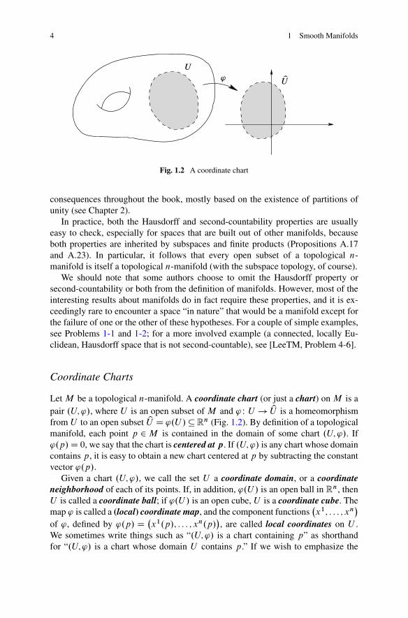
Fig. 1.2 A coordinate chart

consequences throughout the book, mostly based on the existence of partitions ofunity (see Chapter 2).

In practice, both the Hausdorff and second-countability properties are usuallyeasy to check, especially for spaces that are built out of other manifolds, becauseboth properties are inherited by subspaces and finite products (Propositions A.17and A.23). In particular, it follows that every open subset of a topological n-manifold is itself a topological n-manifold (with the subspace topology, of course).

We should note that some authors choose to omit the Hausdorff property orsecond-countability or both from the definition of manifolds. However, most of theinteresting results about manifolds do in fact require these properties, and it is ex-ceedingly rare to encounter a space “in nature” that would be a manifold except forthe failure of one or the other of these hypotheses. For a couple of simple examples,see Problems 1-1 and 1-2; for a more involved example (a connected, locally Eu-clidean, Hausdorff space that is not second-countable), see [LeeTM, Problem 4-6].

Coordinate Charts

Let M be a topological n-manifold. A coordinate chart (or just a chart) on M is apair .U;'/, where U is an open subset of M and ' W U ! yU is a homeomorphismfrom U to an open subset yU D '.U /�Rn (Fig. 1.2). By definition of a topologicalmanifold, each point p 2M is contained in the domain of some chart .U;'/. If'.p/D 0, we say that the chart is centered at p. If .U;'/ is any chart whose domaincontains p, it is easy to obtain a new chart centered at p by subtracting the constantvector '.p/.

Given a chart .U;'/, we call the set U a coordinate domain, or a coordinateneighborhood of each of its points. If, in addition, '.U / is an open ball in Rn, thenU is called a coordinate ball; if '.U / is an open cube, U is a coordinate cube. Themap ' is called a (local) coordinate map, and the component functions

�x1; : : : ; xn

�

of ', defined by '.p/ D�x1.p/; : : : ; xn.p/

�, are called local coordinates on U .

We sometimes write things such as “.U;'/ is a chart containing p” as shorthandfor “.U;'/ is a chart whose domain U contains p.” If we wish to emphasize the


coordinate functions�x1; : : : ; xn

�instead of the coordinate map ', we sometimes

denote the chart by�U;�x1; : : : ; xn

� �or�U;�xi� �

.

Examples of Topological Manifolds

Here are some simple examples.

Example 1.3 (Graphs of Continuous Functions). Let U �Rn be an open subset,and let f W U ! Rk be a continuous function. The graph of f is the subset ofRn �Rk defined by

�.f /D˚.x; y/ 2Rn �Rk W x 2U and y D f .x/

�;

with the subspace topology. Let �1 W Rn �Rk!Rn denote the projection onto thefirst factor, and let ' W �.f /!U be the restriction of �1 to �.f /:

'.x;y/D x; .x;y/ 2 �.f /:

Because ' is the restriction of a continuous map, it is continuous; and it is a home-omorphism because it has a continuous inverse given by '�1.x/D .x; f .x//. Thus�.f / is a topological manifold of dimension n. In fact, �.f / is homeomorphicto U itself, and .�.f /; '/ is a global coordinate chart, called graph coordinates.The same observation applies to any subset of RnCk defined by setting any k ofthe coordinates (not necessarily the last k) equal to some continuous function of theother n, which are restricted to lie in an open subset of Rn. //

Example 1.4 (Spheres). For each integer n� 0, the unit n-sphere Sn is Hausdorffand second-countable because it is a topological subspace of RnC1. To show thatit is locally Euclidean, for each index i D 1; : : : ; nC 1 let UCi denote the subsetof RnC1 where the i th coordinate is positive:

UCi D˚�x1; : : : ; xnC1

�2RnC1 W xi > 0

�:

(See Fig. 1.3.) Similarly, U�i is the set where xi < 0.Let f W Bn!R be the continuous function

f .u/Dp1� juj2:

Then for each i D 1; : : : ; nC 1, it is easy to check that UCi \ Sn is the graph of thefunction

xi D f�x1; : : : ; bxi ; : : : ; xnC1

�;

where the hat indicates that xi is omitted. Similarly, U�i \ Sn is the graph of

xi D�f�x1; : : : ; bxi ; : : : ; xnC1

�:

Thus, each subset U˙i \ Sn is locally Euclidean of dimension n, and the maps'˙i W U

˙i \ Sn! Bn given by

'˙i�x1; : : : ; xnC1

�D�x1; : : : ; bxi ; : : : ; xnC1

�


Fig. 1.3 Charts for Sn

are graph coordinates for Sn. Since each point of Sn is in the domain of at least oneof these 2nC 2 charts, Sn is a topological n-manifold. //

Example 1.5 (Projective Spaces). The n-dimensional real projective space, de-noted by RPn (or sometimes just Pn), is defined as the set of 1-dimensional lin-ear subspaces of RnC1, with the quotient topology determined by the natural map� W RnC1Xf0g!RPn sending each point x 2RnC1Xf0g to the subspace spannedby x. The 2-dimensional projective space RP2 is called the projective plane. Forany point x 2RnC1 X f0g, let Œx�D �.x/ 2RPn denote the line spanned by x.

For each i D 1; : : : ; n C 1, let zUi � RnC1 X f0g be the set where xi ¤ 0,and let Ui D �

�zUi�� RPn. Since zUi is a saturated open subset, Ui is open and

�j zUiW zUi ! Ui is a quotient map (see Theorem A.27). Define a map 'i W Ui !Rn

by

'i�x1; : : : ; xnC1

�D

�x1

xi; : : : ;

xi�1

xi;xiC1

xi; : : : ;

xnC1

xi

�:

This map is well defined because its value is unchanged by multiplying x by anonzero constant. Because 'i ı � is continuous, 'i is continuous by the character-istic property of quotient maps (Theorem A.27). In fact, 'i is a homeomorphism,because it has a continuous inverse given by

'�1i�u1; : : : ; un

�D�u1; : : : ; ui�1; 1; ui ; : : : ; un

�;

as you can check. Geometrically, '.Œx�/ D u means .u; 1/ is the point in RnC1

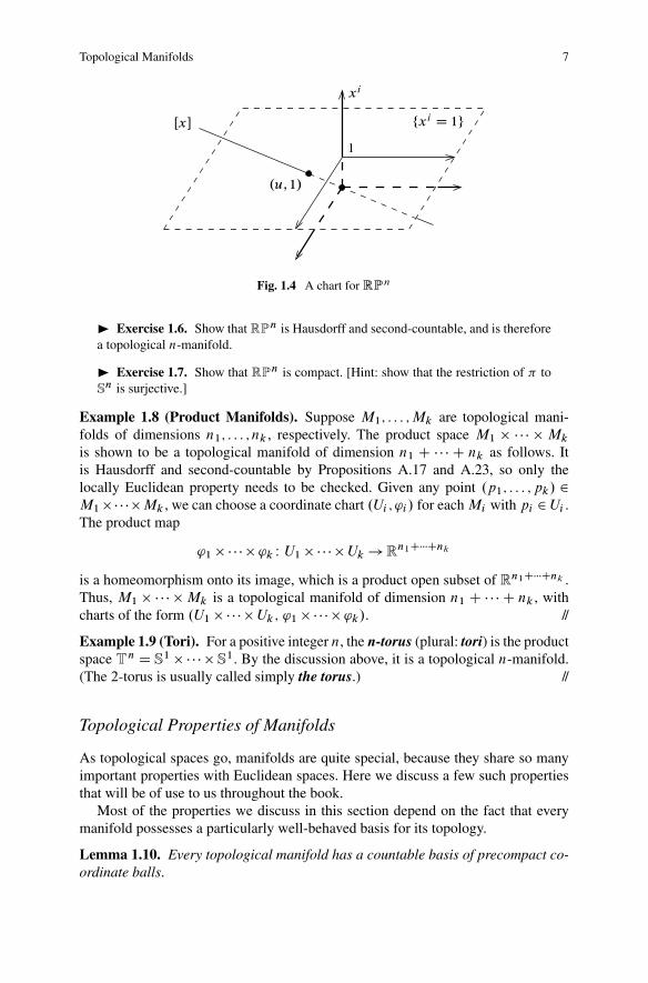
where the line Œx� intersects the affine hyperplane where xi D 1 (Fig. 1.4). Be-cause the sets U1; : : : ;UnC1 cover RPn, this shows that RPn is locally Eu-clidean of dimension n. The Hausdorff and second-countability properties are left asexercises. //


Fig. 1.4 A chart for RPn

I Exercise 1.6. Show that RPn is Hausdorff and second-countable, and is thereforea topological n-manifold.

I Exercise 1.7. Show that RPn is compact. [Hint: show that the restriction of � toSn is surjective.]

Example 1.8 (Product Manifolds). Suppose M1; : : : ;Mk are topological mani-folds of dimensions n1; : : : ; nk , respectively. The product space M1 � � � � � Mk

is shown to be a topological manifold of dimension n1 C � � � C nk as follows. Itis Hausdorff and second-countable by Propositions A.17 and A.23, so only thelocally Euclidean property needs to be checked. Given any point .p1; : : : ; pk/ 2M1� � � ��Mk , we can choose a coordinate chart .Ui ; 'i / for eachMi with pi 2Ui .The product map

'1 � � � � � 'k W U1 � � � � �Uk!Rn1C��Cnk

is a homeomorphism onto its image, which is a product open subset of Rn1C��Cnk .Thus, M1 � � � � �Mk is a topological manifold of dimension n1 C � � � C nk , withcharts of the form .U1 � � � � �Uk ; '1 � � � � � 'k/. //

Example 1.9 (Tori). For a positive integer n, the n-torus (plural: tori) is the productspace Tn D S1 � � � � � S1. By the discussion above, it is a topological n-manifold.(The 2-torus is usually called simply the torus.) //

Topological Properties of Manifolds

As topological spaces go, manifolds are quite special, because they share so manyimportant properties with Euclidean spaces. Here we discuss a few such propertiesthat will be of use to us throughout the book.

Most of the properties we discuss in this section depend on the fact that everymanifold possesses a particularly well-behaved basis for its topology.

Lemma 1.10. Every topological manifold has a countable basis of precompact co-ordinate balls.


Proof. Let M be a topological n-manifold. First we consider the special case inwhich M can be covered by a single chart. Suppose ' W M ! yU � Rn is a globalcoordinate map, and let B be the collection of all open balls Br .x/�Rn such thatr is rational, x has rational coordinates, and Br 0.x/� yU for some r 0 > r . Each suchball is precompact in yU , and it is easy to check that B is a countable basis for thetopology of yU . Because ' is a homeomorphism, it follows that the collection of setsof the form '�1.B/ forB 2B is a countable basis for the topology ofM; consistingof precompact coordinate balls, with the restrictions of ' as coordinate maps.

Now let M be an arbitrary n-manifold. By definition, each point of M is inthe domain of a chart. Because every open cover of a second-countable space hasa countable subcover (Proposition A.16), M is covered by countably many chartsf.Ui ; 'i /g. By the argument in the preceding paragraph, each coordinate domain Uihas a countable basis of coordinate balls that are precompact in Ui , and the union ofall these countable bases is a countable basis for the topology ofM. If V �Ui is oneof these balls, then the closure of V in Ui is compact, and because M is Hausdorff,it is closed in M . It follows that the closure of V in M is the same as its closure inUi , so V is precompact in M as well. �

Connectivity

The existence of a basis of coordinate balls has important consequences for theconnectivity properties of manifolds. Recall that a topological space X is

� connected if there do not exist two disjoint, nonempty, open subsets of X whoseunion is X ;� path-connected if every pair of points in X can be joined by a path in X ; and� locally path-connected if X has a basis of path-connected open subsets.

(See Appendix A.) The following proposition shows that connectivity and path con-nectivity coincide for manifolds.

Proposition 1.11. Let M be a topological manifold.

(a) M is locally path-connected.(b) M is connected if and only if it is path-connected.(c) The components of M are the same as its path components.(d) M has countably many components, each of which is an open subset of M and

a connected topological manifold.

Proof. Since each coordinate ball is path-connected, (a) follows from the fact thatM has a basis of coordinate balls. Parts (b) and (c) are immediate consequences of(a) and Proposition A.43. To prove (d), note that each component is open in M byProposition A.43, so the collection of components is an open cover of M . BecauseM is second-countable, this cover must have a countable subcover. But since thecomponents are all disjoint, the cover must have been countable to begin with, whichis to say thatM has only countably many components. Because the components areopen, they are connected topological manifolds in the subspace topology. �


Local Compactness and Paracompactness

The next topological property of manifolds that we need is local compactness (seeAppendix A for the definition).

Proposition 1.12 (Manifolds Are Locally Compact). Every topological manifoldis locally compact.

Proof. Lemma 1.10 showed that every manifold has a basis of precompact opensubsets. �

Another key topological property possessed by manifolds is called paracompact-ness. It is a consequence of local compactness and second-countability, and in factis one of the main reasons why second-countability is included in the definition ofmanifolds.

LetM be a topological space. A collection X of subsets ofM is said to be locallyfinite if each point of M has a neighborhood that intersects at most finitely manyof the sets in X. Given a cover U of M; another cover V is called a refinement ofU if for each V 2 V there exists some U 2U such that V � U . We say that M isparacompact if every open cover of M admits an open, locally finite refinement.

Lemma 1.13. Suppose X is a locally finite collection of subsets of a topologicalspace M .

(a) The collection˚xX WX 2X

�is also locally finite.

(b)SX2X X D

SX2X

xX .

I Exercise 1.14. Prove the preceding lemma.

Theorem 1.15 (Manifolds Are Paracompact). Every topological manifold isparacompact. In fact, given a topological manifold M; an open cover X of M;and any basis B for the topology of M; there exists a countable, locally finite openrefinement of X consisting of elements of B.

Proof. Given M; X, and B as in the hypothesis of the theorem, let .Kj /1jD1 be anexhaustion of M by compact sets (Proposition A.60). For each j , let Vj DKjC1 XIntKj and Wj D IntKjC2 X Kj�1 (where we interpret Kj as ¿ if j < 1). ThenVj is a compact set contained in the open subset Wj . For each x 2 Vj , there issome Xx 2X containing x, and because B is a basis, there exists Bx 2 B suchthat x 2 Bx � Xx \ Wj . The collection of all such sets Bx as x ranges over Vjis an open cover of Vj , and thus has a finite subcover. The union of all such finitesubcovers as j ranges over the positive integers is a countable open cover of Mthat refines X. Because the finite subcover of Vj consists of sets contained in Wj ,and Wj \Wj 0 D¿ except when j � 2� j 0 � j C 2, the resulting cover is locallyfinite. �

Problem 1-5 shows that, at least for connected spaces, paracompactness can beused as a substitute for second-countability in the definition of manifolds.


Fundamental Groups of Manifolds

The following result about fundamental groups of manifolds will be important inour study of covering manifolds in Chapter 4. For a brief review of the fundamentalgroup, see Appendix A.

Proposition 1.16. The fundamental group of a topological manifold is countable.

Proof. Let M be a topological manifold. By Lemma 1.10, there is a countablecollection B of coordinate balls covering M . For any pair of coordinate ballsB;B 0 2B, the intersection B \B 0 has at most countably many components, eachof which is path-connected. Let X be a countable set containing a point from eachcomponent of B \B 0 for each B;B 0 2B (including B DB 0). For each B 2B andeach x;x0 2X such that x;x0 2B , let hBx;x0 be some path from x to x0 in B .

Since the fundamental groups based at any two points in the same componentof M are isomorphic, and X contains at least one point in each component of M;we may as well choose a point p 2X as base point. Define a special loop to be aloop based at p that is equal to a finite product of paths of the form hBx;x0 . Clearly,the set of special loops is countable, and each special loop determines an elementof �1.M;p/. To show that �1.M;p/ is countable, therefore, it suffices to show thateach element of �1.M;p/ is represented by a special loop.

Suppose f W Œ0; 1�!M is a loop based at p. The collection of components ofsets of the form f �1.B/ as B ranges over B is an open cover of Œ0; 1�, so bycompactness it has a finite subcover. Thus, there are finitely many numbers 0 Da0 < a1 < � � � < ak D 1 such that Œai�1; ai � � f �1.B/ for some B �B. For eachi , let fi be the restriction of f to the interval Œai�1; ai �, reparametrized so that itsdomain is Œ0; 1�, and let Bi 2 B be a coordinate ball containing the image of fi .For each i , we have f .ai / 2 Bi \ BiC1, and there is some xi 2X that lies in thesame component of Bi \BiC1 as f .ai /. Let gi be a path in Bi \BiC1 from xi tof .ai / (Fig. 1.5), with the understanding that x0 D xk D p, and g0 and gk are bothequal to the constant path cp based at p. Then, because xgi � gi is path-homotopic toa constant path (where xgi .t/D gi .1� t/ is the reverse path of gi ),

f f1 � � � � � fk

g0 � f1 � xg1 � g1 � f2 � xg2 � � � � � xgk�1 � gk�1 � fk � xgk

zf1 � zf2 � � � � � zfk ;

where zfi D gi�1 � fi � xgi . For each i , zfi is a path in Bi from xi�1 to xi . SinceBi is simply connected, zfi is path-homotopic to hBixi�1;xi . It follows that f is path-homotopic to a special loop, as claimed. �

Smooth Structures

The definition of manifolds that we gave in the preceding section is sufficient forstudying topological properties of manifolds, such as compactness, connectedness,

Smooth Structures 11

Fig. 1.5 The fundamental group of a manifold is countable

simple connectivity, and the problem of classifying manifolds up to homeomor-phism. However, in the entire theory of topological manifolds there is no men-tion of calculus. There is a good reason for this: however we might try to makesense of derivatives of functions on a manifold, such derivatives cannot be in-variant under homeomorphisms. For example, the map ' W R2 ! R2 given by'.u; v/ D

�u1=3; v1=3

�is a homeomorphism, and it is easy to construct differen-

tiable functions f W R2!R such that f ı ' is not differentiable at the origin. (Thefunction f .x;y/D x is one such.)

To make sense of derivatives of real-valued functions, curves, or maps betweenmanifolds, we need to introduce a new kind of manifold called a smooth manifold. Itwill be a topological manifold with some extra structure in addition to its topology,which will allow us to decide which functions to or from the manifold are smooth.

The definition will be based on the calculus of maps between Euclidean spaces,so let us begin by reviewing some basic terminology about such maps. If U andV are open subsets of Euclidean spaces Rn and Rm, respectively, a functionF W U ! V is said to be smooth (or C1, or infinitely differentiable) if each ofits component functions has continuous partial derivatives of all orders. If in addi-tion F is bijective and has a smooth inverse map, it is called a diffeomorphism.A diffeomorphism is, in particular, a homeomorphism.

A review of some important properties of smooth maps is given in Appendix C.You should be aware that some authors define the word smooth differently—forexample, to mean continuously differentiable or merely differentiable. On the otherhand, some use the word differentiable to mean what we call smooth. Throughoutthis book, smooth is synonymous with C1.

To see what additional structure on a topological manifold might be appropriatefor discerning which maps are smooth, consider an arbitrary topological n-mani-fold M . Each point in M is in the domain of a coordinate map ' W U ! yU � Rn.


Fig. 1.6 A transition map

A plausible definition of a smooth function onM would be to say that f W M !R issmooth if and only if the composite function f ı'�1 W yU !R is smooth in the senseof ordinary calculus. But this will make sense only if this property is independent ofthe choice of coordinate chart. To guarantee this independence, we will restrict ourattention to “smooth charts.” Since smoothness is not a homeomorphism-invariantproperty, the way to do this is to consider the collection of all smooth charts as anew kind of structure on M .

With this motivation in mind, we now describe the details of the construction.Let M be a topological n-manifold. If .U;'/, .V; / are two charts such that

U \ V ¤ ¿, the composite map ı '�1 W '.U \ V /! .U \ V / is called thetransition map from ' to (Fig. 1.6). It is a composition of homeomorphisms, andis therefore itself a homeomorphism. Two charts .U;'/ and .V; / are said to besmoothly compatible if either U \ V D ¿ or the transition map ı '�1 is a dif-feomorphism. Since '.U \ V / and .U \ V / are open subsets of Rn, smoothnessof this map is to be interpreted in the ordinary sense of having continuous partialderivatives of all orders.

We define an atlas for M to be a collection of charts whose domains cover M .An atlas A is called a smooth atlas if any two charts in A are smoothly compatiblewith each other.

To show that an atlas is smooth, we need only verify that each transition map ı'�1 is smooth whenever .U;'/ and .V; / are charts in A; once we have provedthis, it follows that ı '�1 is a diffeomorphism because its inverse

� ı '�1

��1D

' ı �1 is one of the transition maps we have already shown to be smooth. Alterna-tively, given two particular charts .U;'/ and .V; /, it is often easiest to show that


they are smoothly compatible by verifying that ı'�1 is smooth and injective withnonsingular Jacobian at each point, and appealing to Corollary C.36.

Our plan is to define a “smooth structure” on M by giving a smooth atlas, and todefine a function f W M !R to be smooth if and only if f ı '�1 is smooth in thesense of ordinary calculus for each coordinate chart .U;'/ in the atlas. There is oneminor technical problem with this approach: in general, there will be many possibleatlases that give the “same” smooth structure, in that they all determine the samecollection of smooth functions on M . For example, consider the following pair ofatlases on Rn:

A1 D˚�Rn; IdRn

��;

A2 D˚�B1.x/; IdB1.x/

�W x 2Rn

�:

Although these are different smooth atlases, clearly a function f W Rn ! R issmooth with respect to either atlas if and only if it is smooth in the sense of or-dinary calculus.

We could choose to define a smooth structure as an equivalence class of smoothatlases under an appropriate equivalence relation. However, it is more straightfor-ward to make the following definition: a smooth atlas A on M is maximal if it isnot properly contained in any larger smooth atlas. This just means that any chart thatis smoothly compatible with every chart in A is already in A. (Such a smooth atlasis also said to be complete.)

Now we can define the main concept of this chapter. If M is a topological mani-fold, a smooth structure on M is a maximal smooth atlas. A smooth manifold is apair .M;A/, where M is a topological manifold and A is a smooth structure on M .When the smooth structure is understood, we usually omit mention of it and just say“M is a smooth manifold.” Smooth structures are also called differentiable struc-tures or C1 structures by some authors. We also use the term smooth manifoldstructure to mean a manifold topology together with a smooth structure.

We emphasize that a smooth structure is an additional piece of data that mustbe added to a topological manifold before we are entitled to talk about a “smoothmanifold.” In fact, a given topological manifold may have many different smoothstructures (see Example 1.23 and Problem 1-6). On the other hand, it is not alwayspossible to find a smooth structure on a given topological manifold: there exist topo-logical manifolds that admit no smooth structures at all. (The first example was acompact 10-dimensional manifold found in 1960 by Michel Kervaire [Ker60].)

It is generally not very convenient to define a smooth structure by explicitly de-scribing a maximal smooth atlas, because such an atlas contains very many charts.Fortunately, we need only specify some smooth atlas, as the next proposition shows.

Proposition 1.17. Let M be a topological manifold.

(a) Every smooth atlas A for M is contained in a unique maximal smooth atlas,called the smooth structure determined by A.

(b) Two smooth atlases for M determine the same smooth structure if and only iftheir union is a smooth atlas.


Fig. 1.7 Proof of Proposition 1.17(a)

Proof. Let A be a smooth atlas for M; and let SA denote the set of all charts thatare smoothly compatible with every chart in A. To show that SA is a smooth atlas,we need to show that any two charts of SA are smoothly compatible with each other,which is to say that for any .U;'/, .V; / 2 SA, the map ı '�1 W '.U \ V /! .U \ V / is smooth.

Let x D '.p/ 2 '.U \ V / be arbitrary. Because the domains of the charts in A

cover M; there is some chart .W; �/ 2A such that p 2W (Fig. 1.7). Since everychart in SA is smoothly compatible with .W; �/, both of the maps � ı'�1 and ı��1

are smooth where they are defined. Since p 2U \V \W , it follows that ı'�1 D� ı��1

�ı�� ı'�1

�is smooth on a neighborhood of x. Thus, ı'�1 is smooth in

a neighborhood of each point in '.U \V /. Therefore, SA is a smooth atlas. To checkthat it is maximal, just note that any chart that is smoothly compatible with everychart in SA must in particular be smoothly compatible with every chart in A, so it isalready in SA. This proves the existence of a maximal smooth atlas containing A. IfB is any other maximal smooth atlas containing A, each of its charts is smoothlycompatible with each chart in A, so B � SA. By maximality of B, B D SA.

The proof of (b) is left as an exercise. �

I Exercise 1.18. Prove Proposition 1.17(b).

For example, if a topological manifold M can be covered by a single chart, thesmooth compatibility condition is trivially satisfied, so any such chart automaticallydetermines a smooth structure on M .

It is worth mentioning that the notion of smooth structure can be generalizedin several different ways by changing the compatibility requirement for charts.For example, if we replace the requirement that charts be smoothly compatible bythe weaker requirement that each transition map ı '�1 (and its inverse) be of


class C k , we obtain the definition of a C k structure. Similarly, if we require thateach transition map be real-analytic (i.e., expressible as a convergent power series ina neighborhood of each point), we obtain the definition of a real-analytic structure,also called a C! structure. If M has even dimension nD 2m, we can identify R2m

with Cm and require that the transition maps be complex-analytic; this determinesa complex-analytic structure. A manifold endowed with one of these structures iscalled a C k manifold, real-analytic manifold, or complex manifold, respectively.(Note that a C 0 manifold is just a topological manifold.) We do not treat any of theseother kinds of manifolds in this book, but they play important roles in analysis, so itis useful to know the definitions.

Local Coordinate Representations

IfM is a smooth manifold, any chart .U;'/ contained in the given maximal smoothatlas is called a smooth chart, and the corresponding coordinate map ' is called asmooth coordinate map. It is useful also to introduce the terms smooth coordinatedomain or smooth coordinate neighborhood for the domain of a smooth coordinatechart. A smooth coordinate ball means a smooth coordinate domain whose imageunder a smooth coordinate map is a ball in Euclidean space. A smooth coordinatecube is defined similarly.

It is often useful to restrict attention to coordinate balls whose closures sit nicelyinside larger coordinate balls. We say a set B �M is a regular coordinate ball ifthere is a smooth coordinate ball B 0 xB and a smooth coordinate map ' W B 0!Rn

such that for some positive real numbers r < r 0,

'.B/DBr .0/; '�xB�D xBr .0/; and '

�B 0�DBr 0.0/:

Because xB is homeomorphic to xBr .0/, it is compact, and thus every regular coordi-nate ball is precompact in M . The next proposition gives a slight improvement onLemma 1.10 for smooth manifolds. Its proof is a straightforward adaptation of theproof of that lemma.

Proposition 1.19. Every smooth manifold has a countable basis of regular coordi-nate balls.

I Exercise 1.20. Prove Proposition 1.19.

Here is how one usually thinks about coordinate charts on a smooth manifold.Once we choose a smooth chart .U;'/ on M; the coordinate map ' W U ! yU �Rn

can be thought of as giving a temporary identification between U and yU . Using thisidentification, while we work in this chart, we can think of U simultaneously as anopen subset of M and as an open subset of Rn. You can visualize this identificationby thinking of a “grid” drawn on U representing the preimages of the coordinatelines under ' (Fig. 1.8). Under this identification, we can represent a point p 2U by its coordinates

�x1; : : : ; xn

�D '.p/, and think of this n-tuple as being the


Fig. 1.8 A coordinate grid

point p. We typically express this by saying “�x1; : : : ; xn

�is the (local) coordinate

representation for p” or “pD�x1; : : : ; xn

�in local coordinates.”

Another way to look at it is that by means of our identification U $ yU , we canthink of ' as the identity map and suppress it from the notation. This takes a bitof getting used to, but the payoff is a huge simplification of the notation in manysituations. You just need to remember that the identification is in general only local,and depends heavily on the choice of coordinate chart.

You are probably already used to such identifications from your study of mul-tivariable calculus. The most common example is polar coordinates .r; �/ inthe plane, defined implicitly by the relation .x; y/ D .r cos�; r sin�/ (see Exam-ple C.37). On an appropriate open subset such as U D f.x; y/ W x > 0g �R2, .r; �/can be expressed as smooth functions of .x; y/, and the map that sends .x; y/ tothe corresponding .r; �/ is a smooth coordinate map with respect to the standardsmooth structure on R2. Using this map, we can write a given point p 2 U either asp D .x; y/ in standard coordinates or as p D .r; �/ in polar coordinates, where thetwo coordinate representations are related by .r; �/D

�px2C y2; tan�1 y=x

�and

.x; y/D .r cos�; r sin�/. Other polar coordinate charts can be obtained by restrict-ing .r; �/ to other open subsets of R2 X f0g.

The fact that manifolds do not come with any predetermined choice of coordi-nates is both a blessing and a curse. The flexibility to choose coordinates more orless arbitrarily can be a big advantage in approaching problems in manifold the-ory, because the coordinates can often be chosen to simplify some aspect of theproblem at hand. But we pay for this flexibility by being obliged to ensure that anyobjects we wish to define globally on a manifold are not dependent on a particularchoice of coordinates. There are generally two ways of doing this: either by writingdown a coordinate-dependent definition and then proving that the definition givesthe same results in any coordinate chart, or by writing down a definition that is man-ifestly coordinate-independent (often called an invariant definition). We will use thecoordinate-dependent approach in a few circumstances where it is notably simpler,but for the most part we will give coordinate-free definitions whenever possible.The need for such definitions accounts for much of the abstraction of modern man-ifold theory. One of the most important skills you will need to acquire in order touse manifold theory effectively is an ability to switch back and forth easily betweeninvariant descriptions and their coordinate counterparts.

Examples of Smooth Manifolds 17

Examples of Smooth Manifolds

Before proceeding further with the general theory, let us survey some examples ofsmooth manifolds.

Example 1.21 (0-Dimensional Manifolds). A topological manifold M of dimen-sion 0 is just a countable discrete space. For each point p 2M; the only neighbor-hood of p that is homeomorphic to an open subset of R0 is fpg itself, and there isexactly one coordinate map ' W fpg!R0. Thus, the set of all charts on M triviallysatisfies the smooth compatibility condition, and each 0-dimensional manifold hasa unique smooth structure. //

Example 1.22 (Euclidean Spaces). For each nonnegative integer n, the Euclideanspace Rn is a smooth n-manifold with the smooth structure determined by the atlasconsisting of the single chart .Rn; IdRn/. We call this the standard smooth structureon Rn and the resulting coordinate map standard coordinates. Unless we explic-itly specify otherwise, we always use this smooth structure on Rn. With respect tothis smooth structure, the smooth coordinate charts for Rn are exactly those charts.U;'/ such that ' is a diffeomorphism (in the sense of ordinary calculus) from U

to another open subset yU �Rn. //

Example 1.23 (Another Smooth Structure on R). Consider the homeomorphism W R!R given by

.x/D x3: (1.1)

The atlas consisting of the single chart .R; / defines a smooth structure on R.This chart is not smoothly compatible with the standard smooth structure, becausethe transition map IdR ı �1.y/D y1=3 is not smooth at the origin. Therefore, thesmooth structure defined on R by is not the same as the standard one. Usingsimilar ideas, it is not hard to construct many distinct smooth structures on any givenpositive-dimensional topological manifold, as long as it has one smooth structure tobegin with (see Problem 1-6). //

Example 1.24 (Finite-Dimensional Vector Spaces). Let V be a finite-dimensionalreal vector space. Any norm on V determines a topology, which is independentof the choice of norm (Exercise B.49). With this topology, V is a topological n-manifold, and has a natural smooth structure defined as follows. Each (ordered)basis .E1; : : : ;En/ for V defines a basis isomorphism E W Rn! V by

E.x/D

nX

iD1

xiEi :

This map is a homeomorphism, so�V;E�1

�is a chart. If

�zE1; : : : ; zEn

�is any other

basis and zE.x/DPj x

j zEj is the corresponding isomorphism, then there is some

invertible matrix�Aji

�such that Ei D

Pj A

jizEj for each i . The transition map

between the two charts is then given by zE�1 ıE.x/D zx, where zx D�zx1; : : : ; zxn

�


is determined bynX

jD1

zxj zEj D

nX

iD1

xiEi D

nX

i;jD1

xiAjizEj :

It follows that zxj DPi A

ji xi . Thus, the map sending x to zx is an invertible linear

map and hence a diffeomorphism, so any two such charts are smoothly compatible.The collection of all such charts thus defines a smooth structure, called the standardsmooth structure on V . //

The Einstein Summation Convention

This is a good place to pause and introduce an important notational convention thatis commonly used in the study of smooth manifolds. Because of the proliferationof summations such as

Pi xiEi in this subject, we often abbreviate such a sum by

omitting the summation sign, as in

E.x/D xiEi ; an abbreviation for E.x/DnX

iD1

xiEi :

We interpret any such expression according to the following rule, called the Einsteinsummation convention: if the same index name (such as i in the expression above)appears exactly twice in any monomial term, once as an upper index and once asa lower index, that term is understood to be summed over all possible values ofthat index, generally from 1 to the dimension of the space in question. This simpleidea was introduced by Einstein to reduce the complexity of expressions arisingin the study of smooth manifolds by eliminating the necessity of explicitly writingsummation signs. We use the summation convention systematically throughout thebook (except in the appendices, which many readers will look at before the rest ofthe book).

Another important aspect of the summation convention is the positions of theindices. We always write basis vectors (such as Ei ) with lower indices, and com-ponents of a vector with respect to a basis (such as xi ) with upper indices. Theseindex conventions help to ensure that, in summations that make mathematical sense,each index to be summed over typically appears twice in any given term, once as alower index and once as an upper index. Any index that is implicitly summed overis a “dummy index,” meaning that the value of such an expression is unchanged if adifferent name is substituted for each dummy index. For example, xiEi and xjEjmean exactly the same thing.

Since the coordinates of a point�x1; : : : ; xn

�2Rn are also its components with

respect to the standard basis, in order to be consistent with our convention of writingcomponents of vectors with upper indices, we need to use upper indices for these co-ordinates, and we do so throughout this book. Although this may seem awkward atfirst, in combination with the summation convention it offers enormous advantages


when we work with complicated indexed sums, not the least of which is that expres-sions that are not mathematically meaningful often betray themselves quickly byviolating the index convention. (The main exceptions are expressions involving theEuclidean dot product x � y D

Pi xiyi , in which the same index appears twice in

the upper position, and the standard symplectic form on R2n, which we will definein Chapter 22. We always explicitly write summation signs in such expressions.)

More Examples

Now we continue with our examples of smooth manifolds.

Example 1.25 (Spaces of Matrices). Let M.m � n;R/ denote the set of m � nmatrices with real entries. Because it is a real vector space of dimension mn undermatrix addition and scalar multiplication, M.m�n;R/ is a smoothmn-dimensionalmanifold. (In fact, it is often useful to identify M.m � n;R/ with Rmn, just bystringing all the matrix entries out in a single row.) Similarly, the space M.m�n;C/of m � n complex matrices is a vector space of dimension 2mn over R, and thusa smooth manifold of dimension 2mn. In the special case in which mD n (squarematrices), we abbreviate M.n � n;R/ and M.n � n;C/ by M.n;R/ and M.n;C/,respectively. //

Example 1.26 (Open Submanifolds). Let U be any open subset of Rn. Then U isa topological n-manifold, and the single chart .U; IdU / defines a smooth structureon U .

More generally, let M be a smooth n-manifold and let U �M be any opensubset. Define an atlas on U by

AU D˚smooth charts .V;'/ for M such that V �U

�:

Every point p 2 U is contained in the domain of some chart .W;'/ forM ; if we setV DW \U , then .V;'jV / is a chart in AU whose domain contains p. Therefore,U is covered by the domains of charts in AU , and it is easy to verify that this isa smooth atlas for U . Thus any open subset of M is itself a smooth n-manifoldin a natural way. Endowed with this smooth structure, we call any open subset anopen submanifold of M . (We will define a more general class of submanifolds inChapter 5.) //

Example 1.27 (The General Linear Group). The general linear group GL.n;R/is the set of invertible n�nmatrices with real entries. It is a smooth n2-dimensionalmanifold because it is an open subset of the n2-dimensional vector space M.n;R/,namely the set where the (continuous) determinant function is nonzero. //

Example 1.28 (Matrices of Full Rank). The previous example has a natural gener-alization to rectangular matrices of full rank. Supposem< n, and let Mm.m�n;R/denote the subset of M.m � n;R/ consisting of matrices of rank m. If A is an ar-bitrary such matrix, the fact that rankA D m means that A has some nonsingularm �m submatrix. By continuity of the determinant function, this same submatrix


has nonzero determinant on a neighborhood of A in M.m � n;R/, which impliesthat A has a neighborhood contained in Mm.m� n;R/. Thus, Mm.m� n;R/ is anopen subset of M.m� n;R/, and therefore is itself a smooth mn-dimensional man-ifold. A similar argument shows that Mn.m�n;R/ is a smooth mn-manifold whenn <m. //

Example 1.29 (Spaces of Linear Maps). Suppose V andW are finite-dimensionalreal vector spaces, and let L.V IW / denote the set of linear maps from V toW . Thenbecause L.V IW / is itself a finite-dimensional vector space (whose dimension is theproduct of the dimensions of V and W ), it has a natural smooth manifold structureas in Example 1.24. One way to put global coordinates on it is to choose bases for VandW , and represent each T 2 L.V IW / by its matrix, which yields an isomorphismof L.V IW / with M.m� n;R/ for mD dimW and nD dimV . //

Example 1.30 (Graphs of Smooth Functions). If U � Rn is an open subset andf W U !Rk is a smooth function, we have already observed above (Example 1.3)that the graph of f is a topological n-manifold in the subspace topology. Since�.f / is covered by the single graph coordinate chart ' W �.f /!U (the restrictionof �1), we can put a canonical smooth structure on �.f / by declaring the graphcoordinate chart .�.f /; '/ to be a smooth chart. //

Example 1.31 (Spheres). We showed in Example 1.4 that the n-sphere Sn �RnC1

is a topological n-manifold. We put a smooth structure on Sn as follows. For eachi D 1; : : : ; nC 1, let

�U˙i ; '

˙i

�denote the graph coordinate charts we constructed

in Example 1.4. For any distinct indices i and j , the transition map '˙i ı�'˙j��1 is

easily computed. In the case i < j , we get

'˙i ı�'˙j��1 �

u1; : : : ; un�Du1; : : : ; bui ; : : : ;˙

p1� juj2; : : : ; un

(with the square root in the j th position), and a similar formula holds when i > j .When i D j , an even simpler computation gives 'Ci ı

�'�i��1 D '�i ı

�'Ci��1 D

IdBn . Thus, the collection of charts˚�U˙i ; '

˙i

��is a smooth atlas, and so defines a

smooth structure on Sn. We call this its standard smooth structure. //

Example 1.32 (Level Sets). The preceding example can be generalized as fol-lows. Suppose U � Rn is an open subset and ˚ W U ! R is a smooth function.For any c 2 R, the set ˚�1.c/ is called a level set of ˚ . Choose some c 2 R, letM D ˚�1.c/, and suppose it happens that the total derivative D˚.a/ is nonzerofor each a 2 ˚�1.c/. Because D˚.a/ is a row matrix whose entries are the partialderivatives .@˚[email protected]/; : : : ; @˚[email protected]//, for each a 2M there is some i such that@˚=@xi .a/¤ 0. It follows from the implicit function theorem (Theorem C.40, withxi playing the role of y) that there is a neighborhood U0 of a such that M \U0 canbe expressed as a graph of an equation of the form

xi D fx1; : : : ; bxi ; : : : ; xn

;

for some smooth real-valued function f defined on an open subset of Rn�1. There-fore, arguing just as in the case of the n-sphere, we see that M is a topological


manifold of dimension .n � 1/, and has a smooth structure such that each of thegraph coordinate charts associated with a choice of f as above is a smooth chart.In Chapter 5, we will develop the theory of smooth submanifolds, which is a far-reaching generalization of this construction. //

Example 1.33 (Projective Spaces). The n-dimensional real projective space RPn

is a topological n-manifold by Example 1.5. Let us check that the coordinate charts.Ui ; 'i / constructed in that example are all smoothly compatible. Assuming for con-venience that i > j , it is straightforward to compute that

'j ı '�1i

�u1; : : : ; un

�D

�u1

uj; : : : ;

uj�1

uj;ujC1

uj; : : : ;

ui�1

uj;1

uj;ui

uj; : : : ;

un

uj

�;

which is a diffeomorphism from 'i .Ui \Uj / to 'j .Ui \Uj /. //

Example 1.34 (Smooth Product Manifolds). IfM1; : : : ;Mk are smooth manifoldsof dimensions n1; : : : ; nk , respectively, we showed in Example 1.8 that the productspace M1 � � � � �Mk is a topological manifold of dimension n1 C � � � C nk , withcharts of the form .U1 � � � � �Uk ; '1 � � � � � 'k/. Any two such charts are smoothlycompatible because, as is easily verified,

. 1 � � � � � k/ ı .'1 � � � � � 'k/�1 D

� 1 ı '

�11

��

� k ı '

�1k

�;

which is a smooth map. This defines a natural smooth manifold structure on theproduct, called the product smooth manifold structure. For example, this yields asmooth manifold structure on the n-torus Tn D S1 � � � � � S1. //

In each of the examples we have seen so far, we constructed a smooth manifoldstructure in two stages: we started with a topological space and checked that it wasa topological manifold, and then we specified a smooth structure. It is often moreconvenient to combine these two steps into a single construction, especially if westart with a set that is not already equipped with a topology. The following lemmaprovides a shortcut—it shows how, given a set with suitable “charts” that overlapsmoothly, we can use the charts to define both a topology and a smooth structure onthe set.

Lemma 1.35 (Smooth Manifold Chart Lemma). Let M be a set, and suppose weare given a collection fU˛g of subsets ofM together with maps '˛ W U˛!Rn, suchthat the following properties are satisfied:

(i) For each ˛, '˛ is a bijection between U˛ and an open subset '˛.U˛/�Rn.(ii) For each ˛ and ˇ, the sets '˛.U˛ \Uˇ / and 'ˇ .U˛ \Uˇ / are open in Rn.

(iii) Whenever U˛ \Uˇ ¤¿, the map 'ˇ ı '�1˛ W '˛.U˛ \Uˇ /! 'ˇ .U˛ \Uˇ / issmooth.

(iv) Countably many of the sets U˛ cover M .(v) Whenever p;q are distinct points in M; either there exists some U˛ containing

both p and q or there exist disjoint sets U˛;Uˇ with p 2U˛ and q 2 Uˇ .

ThenM has a unique smooth manifold structure such that each .U˛; '˛/ is a smoothchart.


Fig. 1.9 The smooth manifold chart lemma

Proof. We define the topology by taking all sets of the form '�1˛ .V /, with V anopen subset of Rn, as a basis. To prove that this is a basis for a topology, we need toshow that for any point p in the intersection of two basis sets '�1˛ .V / and '�1

ˇ.W /,

there is a third basis set containing p and contained in the intersection. It sufficesto show that '�1˛ .V / \ '�1

ˇ.W / is itself a basis set (Fig. 1.9). To see this, observe

that (iii) implies that�'ˇ ı '

�1˛

��1.W / is an open subset of '˛.U˛ \Uˇ /, and (ii)

implies that this set is also open in Rn. It follows that

'�1˛ .V /\ '�1ˇ .W /D '�1˛�V \

�'ˇ ı '

�1˛

��1.W /

�

is also a basis set, as claimed.Each map '˛ is then a homeomorphism onto its image (essentially by definition),

so M is locally Euclidean of dimension n. The Hausdorff property follows easilyfrom (v), and second-countability follows from (iv) and the result of Exercise A.22,because each U˛ is second-countable. Finally, (iii) guarantees that the collectionf.U˛; '˛/g is a smooth atlas. It is clear that this topology and smooth structure arethe unique ones satisfying the conclusions of the lemma. �

Example 1.36 (Grassmann Manifolds). Let V be an n-dimensional real vectorspace. For any integer 0� k � n, we let Gk.V / denote the set of all k-dimensionallinear subspaces of V . We will show that Gk.V / can be naturally given the struc-ture of a smooth manifold of dimension k.n� k/. With this structure, it is called aGrassmann manifold, or simply a Grassmannian. In the special case V DRn, theGrassmannian Gk

�Rn�

is often denoted by some simpler notation such as Gk;n orG.k; n/. Note that G1

�RnC1

�is exactly the n-dimensional projective space RPn.


The construction of a smooth structure on Gk.V / is somewhat more involvedthan the ones we have done so far, but the basic idea is just to use linear algebrato construct charts for Gk.V /, and then apply the smooth manifold chart lemma.We will give a shorter proof that Gk.V / is a smooth manifold in Chapter 21 (seeExample 21.21).

Let P and Q be any complementary subspaces of V of dimensions k and n� k,respectively, so that V decomposes as a direct sum: V D P ˚Q. The graph of anylinear map X W P !Q can be identified with a k-dimensional subspace �.X/� V ,defined by

�.X/D fvCXv W v 2 P g:

Any such subspace has the property that its intersection withQ is the zero subspace.Conversely, any subspace S � V that intersects Q trivially is the graph of a uniquelinear map X W P ! Q, which can be constructed as follows: let �P W V ! P

and �Q W V !Q be the projections determined by the direct sum decomposition;then the hypothesis implies that �P jS is an isomorphism from S to P . Therefore,X D .�QjS /ı .�P jS /

�1 is a well-defined linear map from P toQ, and it is straight-forward to check that S is its graph.

Let L.P IQ/ denote the vector space of linear maps from P to Q, and letUQ denote the subset of Gk.V / consisting of k-dimensional subspaces whoseintersections with Q are trivial. The assignment X 7! �.X/ defines a map� W L.P IQ/ ! UQ, and the discussion above shows that � is a bijection. Let' D ��1 W UQ ! L.P IQ/. By choosing bases for P and Q, we can identifyL.P IQ/ with M..n� k/� k;R/ and hence with Rk.n�k/, and thus we can think of.UQ; '/ as a coordinate chart. Since the image of each such chart is all of L.P IQ/,condition (i) of Lemma 1.35 is clearly satisfied.

Now let .P 0;Q0/ be any other such pair of subspaces, and let �P 0 , �Q0 be the cor-responding projections and '0 W UQ0 ! L.P 0IQ0/ the corresponding map. The set'.UQ \UQ0/� L.P IQ/ consists of all linear maps X W P !Q whose graphs in-tersectQ0 trivially. To see that this set is open in L.P IQ/, for eachX 2 L.P IQ/, letIX W P ! V be the map IX .v/D vCXv, which is a bijection from P to the graphof X . Because �.X/D ImIX and Q0 D Ker�P 0 , it follows from Exercise B.22(d)that the graph of X intersects Q0 trivially if and only if �P 0 ı IX has full rank.Because the matrix entries of �P 0 ı IX (with respect to any bases) depend continu-ously on X , the result of Example 1.28 shows that the set of all such X is open inL.P IQ/. Thus property (ii) in the smooth manifold chart lemma holds.

We need to show that the transition map '0 ı '�1 is smooth on '.UQ \ UQ0/.Suppose X 2 '.UQ \ UQ0/� L.P IQ/ is arbitrary, and let S denote the subspace�.X/� V . If we put X 0 D '0 ı '�1.X/, then as above, X 0 D .�Q0 jS / ı .�P 0 jS /�1

(see Fig. 1.10). To relate this map to X , note that IX W P ! S is an isomorphism, sowe can write

X 0 D .�Q0 jS / ı IX ı .IX /�1 ı .�P 0 jS /

�1 D .�Q0 ı IX / ı .�P 0 ı IX /�1:


Fig. 1.10 Smooth compatibility of coordinates on Gk.V /

To show that this depends smoothly on X , define linear maps A W P ! P 0,B W P !Q0, C W Q! P 0, and D W Q!Q0 as follows:

AD �P 0ˇˇP; B D �Q0

ˇˇP; C D �P 0

ˇˇQ; D D �Q0

ˇˇQ:

Then for v 2 P , we have

.�P 0 ı IX /vD .ACCX/v; .�Q0 ı IX /vD .B CDX/v;

from which it follows that X 0 D .B CDX/.AC CX/�1. Once we choose basesfor P , Q, P 0, and Q0, all of these linear maps are represented by matrices. Becausethe matrix entries of .AC CX/�1 are rational functions of those of AC CX byCramer’s rule, it follows that the matrix entries of X 0 depend smoothly on those ofX . This proves that '0 ı '�1 is a smooth map, so the charts we have constructedsatisfy condition (iii) of Lemma 1.35.

To check condition (iv), we just note that Gk.V / can in fact be covered by finitelymany of the sets UQ: for example, if .E1; : : : ;En/ is any fixed basis for V , anypartition of the basis elements into two subsets containing k and n � k elementsdetermines appropriate subspaces P and Q, and any subspace S must have trivialintersection with Q for at least one of these partitions (see Exercise B.9). Thus,Gk.V / is covered by the finitely many charts determined by all possible partitionsof a fixed basis.

Finally, the Hausdorff condition (v) is easily verified by noting that for any two k-dimensional subspaces P;P 0 � V , it is possible to find a subspace Q of dimensionn � k whose intersections with both P and P 0 are trivial, and then P and P 0 areboth contained in the domain of the chart determined by, say, .P;Q/. //

Manifolds with Boundary

In many important applications of manifolds, most notably those involving integra-tion, we will encounter spaces that would be smooth manifolds except that they

Manifolds with Boundary 25

Fig. 1.11 A manifold with boundary

have a “boundary” of some sort. Simple examples of such spaces include closedintervals in R, closed balls in Rn, and closed hemispheres in Sn. To accommodatesuch spaces, we need to extend our definition of manifolds.

Points in these spaces will have neighborhoods modeled either on open subsetsof Rn or on open subsets of the closed n-dimensional upper half-space Hn �Rn,defined as

Hn D˚�x1; : : : ; xn

�2Rn W xn � 0

�:

We will use the notations IntHn and @Hn to denote the interior and boundary of Hn,respectively, as a subset of Rn. When n > 0, this means

IntHn D˚�x1; : : : ; xn

�2Rn W xn > 0

�;

@Hn D˚�x1; : : : ; xn

�2Rn W xn D 0

�:

In the nD 0 case, H0 DR0 D f0g, so IntH0 DR0 and @H0 D¿.An n-dimensional topological manifold with boundary is a second-countable

Hausdorff space M in which every point has a neighborhood homeomorphic eitherto an open subset of Rn or to a (relatively) open subset of Hn (Fig. 1.11). An opensubset U �M together with a map ' W U !Rn that is a homeomorphism onto anopen subset of Rn or Hn will be called a chart for M , just as in the case of man-ifolds. When it is necessary to make the distinction, we will call .U;'/ an interiorchart if '.U / is an open subset of Rn (which includes the case of an open subsetof Hn that does not intersect @Hn), and a boundary chart if '.U / is an open subsetof Hn such that '.U / \ @Hn ¤ ¿. A boundary chart whose image is a set of theform Br .x/\Hn for some x 2 @Hn and r > 0 is called a coordinate half-ball.

A point p 2M is called an interior point of M if it is in the domain of someinterior chart. It is a boundary point of M if it is in the domain of a boundary chartthat sends p to @Hn. The boundary of M (the set of all its boundary points) isdenoted by @M ; similarly, its interior, the set of all its interior points, is denoted byIntM .

It follows from the definition that each point p 2M is either an interior point or aboundary point: if p is not a boundary point, then either it is in the domain of an in-terior chart or it is in the domain of a boundary chart .U;'/ such that '.p/ … @Hn,


in which case the restriction of ' to U \ '�1�IntHn

�is an interior chart whose

domain contains p. However, it is not obvious that a given point cannot be simulta-neously an interior point with respect to one chart and a boundary point with respectto another. In fact, this cannot happen, but the proof requires more machinery thanwe have available at this point. For convenience, we state the theorem here.

Theorem 1.37 (Topological Invariance of the Boundary). If M is a topologicalmanifold with boundary, then each point of M is either a boundary point or aninterior point, but not both. Thus @M and IntM are disjoint sets whose union isM .

For the proof, see Problem 17-9. Later in this chapter, we will prove a weakerversion of this result for smooth manifolds with boundary (Theorem 1.46), whichwill be sufficient for most of our purposes.

Be careful to observe the distinction between these new definitions of the termsboundary and interior and their usage to refer to the boundary and interior of a sub-set of a topological space. A manifold with boundary may have nonempty boundaryin this new sense, irrespective of whether it has a boundary as a subset of some othertopological space. If we need to emphasize the difference between the two notionsof boundary, we will use the terms topological boundary and manifold boundaryas appropriate. For example, the closed unit ball xBn is a manifold with boundary(see Problem 1-11), whose manifold boundary is Sn�1. Its topological boundary asa subset of Rn happens to be the sphere as well. However, if we think of xBn asa topological space in its own right, then as a subset of itself, it has empty topo-logical boundary. And if we think of it as a subset of RnC1 (considering Rn as asubset of RnC1 in the obvious way), its topological boundary is all of xBn. Note thatHn is itself a manifold with boundary, and its manifold boundary is the same as itstopological boundary as a subset of Rn. Every interval in R is a 1-manifold withboundary, whose manifold boundary consists of its endpoints (if any).

The nomenclature for manifolds with boundary is traditional and well estab-lished, but it must be used with care. Despite their name, manifolds with boundaryare not in general manifolds, because boundary points do not have locally Euclideanneighborhoods. (This is a consequence of the theorem on invariance of the bound-ary.) Moreover, a manifold with boundary might have empty boundary—there isnothing in the definition that requires the boundary to be a nonempty set. On theother hand, a manifold is also a manifold with boundary, whose boundary is empty.Thus, every manifold is a manifold with boundary, but a manifold with boundary isa manifold if and only if its boundary is empty (see Proposition 1.38 below).

Even though the term manifold with boundary encompasses manifolds as well,we will often use redundant phrases such as manifold without boundary if we wishto emphasize that we are talking about a manifold in the original sense, and man-ifold with or without boundary to refer to a manifold with boundary if we wishemphasize that the boundary might be empty. (The latter phrase will often appearwhen our primary interest is in manifolds, but the results being discussed are just aseasy to state and prove in the more general case of manifolds with boundary.) Notethat the word “manifold” without further qualification always means a manifold

Manifolds with Boundary 27

without boundary. In the literature, you will also encounter the terms closed mani-fold to mean a compact manifold without boundary, and open manifold to mean anoncompact manifold without boundary.

Proposition 1.38. Let M be a topological n-manifold with boundary.

(a) IntM is an open subset of M and a topological n-manifold without boundary.(b) @M is a closed subset of M and a topological .n � 1/-manifold without

boundary.(c) M is a topological manifold if and only if @M D¿.(d) If nD 0, then @M D¿ and M is a 0-manifold.

I Exercise 1.39. Prove the preceding proposition. For this proof, you may use thetheorem on topological invariance of the boundary when necessary. Which parts re-quire it?

The topological properties of manifolds that we proved earlier in the chapter havenatural extensions to manifolds with boundary, with essentially the same proofs asin the manifold case. For the record, we state them here.

Proposition 1.40. Let M be a topological manifold with boundary.

(a) M has a countable basis of precompact coordinate balls and half-balls.(b) M is locally compact.(c) M is paracompact.(d) M is locally path-connected.(e) M has countably many components, each of which is an open subset of M and

a connected topological manifold with boundary.(f) The fundamental group of M is countable.

I Exercise 1.41. Prove the preceding proposition.

Smooth Structures on Manifolds with Boundary

To see how to define a smooth structure on a manifold with boundary, recall that amap from an arbitrary subset A � Rn to Rk is said to be smooth if in a neighbor-hood of each point of A it admits an extension to a smooth map defined on an opensubset of Rn (see Appendix C, p. 645). Thus, if U is an open subset of Hn, a mapF W U !Rk is smooth if for each x 2 U , there exists an open subset zU �Rn con-taining x and a smooth map zF W zU !Rk that agrees with F on zU \Hn (Fig. 1.12).If F is such a map, the restriction of F to U \ IntHn is smooth in the usual sense.By continuity, all partial derivatives of F at points of U \ @Hn are determined bytheir values in IntHn, and therefore in particular are independent of the choice ofextension. It is a fact (which we will neither prove nor use) that F W U ! Rk issmooth in this sense if and only if F is continuous, F jU\IntHn is smooth, and thepartial derivatives of F jU\IntHn of all orders have continuous extensions to all of U .(One direction is obvious; the other direction depends on a lemma of Émile Borel,which shows that there is a smooth function defined in the lower half-space whosederivatives all match those of F on U \ @Hn. See, e.g., [Hör90, Thm. 1.2.6].)


Fig. 1.12 Smoothness of maps on open subsets of Hn

For example, let B2 � R2 be the open unit disk, let U D B2 \H2, and definef W U !R by f .x;y/D

p1� x2 � y2. Because f extends smoothly to all of B2

(by the same formula), f is a smooth function on U . On the other hand, althoughg.x;y/ D

py is continuous on U and smooth in U \ IntH2, it has no smooth

extension to any neighborhood of the origin in R2 because @g=@y!1 as y! 0.Thus g is not smooth on U .

Now let M be a topological manifold with boundary. As in the manifold case,a smooth structure for M is defined to be a maximal smooth atlas—a collectionof charts whose domains cover M and whose transition maps (and their inverses)are smooth in the sense just described. With such a structure, M is called a smoothmanifold with boundary. Every smooth manifold is automatically a smooth mani-fold with boundary (whose boundary is empty).

Just as for smooth manifolds, if M is a smooth manifold with boundary, anychart in the given smooth atlas is called a smooth chart for M . Smooth coordinateballs, smooth coordinate half-balls, and regular coordinate balls inM are definedin the obvious ways. In addition, a subset B �M is called a regular coordinatehalf-ball if there is a smooth coordinate half-ball B 0 xB and a smooth coordinatemap ' W B 0!Hn such that for some r 0 > r > 0 we have

'.B/DBr .0/\Hn; '�xB�D xBr .0/\Hn; and '

�B 0�DBr 0.0/\Hn:

I Exercise 1.42. Show that every smooth manifold with boundary has a countablebasis consisting of regular coordinate balls and half-balls.

I Exercise 1.43. Show that the smooth manifold chart lemma (Lemma 1.35) holdswith “Rn” replaced by “Rn or Hn” and “smooth manifold” replaced by “smoothmanifold with boundary.”

I Exercise 1.44. Suppose M is a smooth n-manifold with boundary and U is anopen subset of M . Prove the following statements:

(a) U is a topological n-manifold with boundary, and the atlas consisting of all smoothcharts .V;'/ for M such that V � U defines a smooth structure on U . With thistopology and smooth structure, U is called an open submanifold with boundary.

(b) If U � IntM; then U is actually a smooth manifold (without boundary); in thiscase we call it an open submanifold of M .

(c) IntM is an open submanifold of M (without boundary).

Problems 29

One important result about smooth manifolds that does not extend directly tosmooth manifolds with boundary is the construction of smooth structures on finiteproducts (see Example 1.8). Because a product of half-spaces Hn �Hm is not itselfa half-space, a finite product of smooth manifolds with boundary cannot generallybe considered as a smooth manifold with boundary. (Instead, it is an example of asmooth manifold with corners, which we will study in Chapter 16.) However, we dohave the following result.

Proposition 1.45. Suppose M1; : : : ;Mk are smooth manifolds and N is a smoothmanifold with boundary. ThenM1�� Mk �N is a smooth manifold with bound-ary, and @.M1 � � � � �Mk �N/DM1 � � � � �Mk � @N .

Proof. Problem 1-12. �

For smooth manifolds with boundary, the following result is often an adequatesubstitute for the theorem on invariance of the boundary.

Theorem 1.46 (Smooth Invariance of the Boundary). Suppose M is a smoothmanifold with boundary and p 2M . If there is some smooth chart .U;'/ for Msuch that '.U /�Hn and '.p/ 2 @Hn, then the same is true for every smooth chartwhose domain contains p.

Proof. Suppose on the contrary that p is in the domain of a smooth interior chart.U; / and also in the domain of a smooth boundary chart .V;'/ such that '.p/ 2@Hn. Let � D ' ı �1 denote the transition map; it is a homeomorphism from .U \V / to '.U \V /. The smooth compatibility of the charts ensures that both �and ��1 are smooth, in the sense that locally they can be extended, if necessary, tosmooth maps defined on open subsets of Rn.

Write x0 D .p/ and y0 D '.p/D �.x0/. There is some neighborhoodW of y0in Rn and a smooth function � W W !Rn that agrees with ��1 on W \ '.U \ V /.On the other hand, because we are assuming that is an interior chart, there isan open Euclidean ball B that is centered at x0 and contained in '.U \ V /, so �itself is smooth on B in the ordinary sense. After shrinking B if necessary, we mayassume that B � ��1.W /. Then � ı � jB D ��1 ı � jB D IdB , so it follows from thechain rule that D�.�.x// ıD�.x/ is the identity map for each x 2B . Since D�.x/is a square matrix, this implies that it is nonsingular. It follows from Corollary C.36that � (considered as a map from B to Rn) is an open map, so �.B/ is an opensubset of Rn that contains y0 D '.p/ and is contained in '.V /. This contradicts theassumption that '.V /�Hn and '.p/ 2 @Hn. �

Problems

1-1. Let X be the set of all points .x; y/ 2 R2 such that y D˙1, and let M bethe quotient of X by the equivalence relation generated by .x;�1/ .x; 1/for all x ¤ 0. Show that M is locally Euclidean and second-countable, butnot Hausdorff. (This space is called the line with two origins.)


1-2. Show that a disjoint union of uncountably many copies of R is locallyEuclidean and Hausdorff, but not second-countable.

1-3. A topological space is said to be � -compact if it can be expressed asa union of countably many compact subspaces. Show that a locally Eu-clidean Hausdorff space is a topological manifold if and only if it is � -compact.

1-4. Let M be a topological manifold, and let U be an open cover of M .(a) Assuming that each set in U intersects only finitely many others, show

that U is locally finite.(b) Give an example to show that the converse to (a) may be false.(c) Now assume that the sets in U are precompact inM; and prove the con-

verse: if U is locally finite, then each set in U intersects only finitelymany others.

1-5. SupposeM is a locally Euclidean Hausdorff space. Show thatM is second-countable if and only if it is paracompact and has countably many connectedcomponents. [Hint: assumingM is paracompact, show that each componentof M has a locally finite cover by precompact coordinate domains, and ex-tract from this a countable subcover.]

1-6. Let M be a nonempty topological manifold of dimension n � 1. If M hasa smooth structure, show that it has uncountably many distinct ones. [Hint:first show that for any s > 0, Fs.x/ D jxjs�1x defines a homeomorphismfrom Bn to itself, which is a diffeomorphism if and only if s D 1.]

1-7. Let N denote the north pole .0; : : : ; 0; 1/ 2 Sn � RnC1, and let S de-note the south pole .0; : : : ; 0;�1/. Define the stereographic projection� W Sn X fN g!Rn by

��x1; : : : ; xnC1

�D.x1; : : : ; xn/

1� xnC1:

Let z�.x/D��.�x/ for x 2 Sn X fSg.(a) For any x 2 Sn X fN g, show that �.x/ D u, where .u; 0/ is the point

where the line through N and x intersects the linear subspace wherexnC1 D 0 (Fig. 1.13). Similarly, show that z�.x/ is the point where theline through S and x intersects the same subspace. (For this reason, z�is called stereographic projection from the south pole.)

(b) Show that � is bijective, and

��1�u1; : : : ; un

�D.2u1; : : : ; 2un; juj2 � 1/

juj2C 1:

(c) Compute the transition map z� ı ��1 and verify that the atlas consistingof the two charts .Sn X fN g; �/ and .Sn X fSg; z�/ defines a smoothstructure on Sn. (The coordinates defined by � or z� are called stereo-graphic coordinates.)

(d) Show that this smooth structure is the same as the one defined inExample 1.31.

(Used on pp. 201, 269, 301, 345, 347, 450.)

Problems 31

Fig. 1.13 Stereographic projection

1-8. By identifying R2 with C, we can think of the unit circle S1 as a subset ofthe complex plane. An angle function on a subset U � S1 is a continuousfunction � W U !R such that ei�.z/ D z for all z 2 U . Show that there existsan angle function � on an open subset U � S1 if and only if U ¤ S1. Forany such angle function, show that .U; �/ is a smooth coordinate chart forS1 with its standard smooth structure. (Used on pp. 37, 152, 176.)

1-9. Complex projective n-space, denoted by CPn, is the set of all 1-dimensionalcomplex-linear subspaces of CnC1, with the quotient topology inheritedfrom the natural projection � W CnC1 X f0g ! CPn. Show that CPn is acompact 2n-dimensional topological manifold, and show how to give it asmooth structure analogous to the one we constructed for RPn. (We use thecorrespondence

�x1C iy1; : : : ; xnC1C iynC1

�$�x1; y1; : : : ; xnC1; ynC1

�

to identify CnC1 with R2nC2.) (Used on pp. 48, 96, 172, 560, 561.)

1-10. Let k and n be integers satisfying 0 < k < n, and let P;Q � Rn be thelinear subspaces spanned by .e1; : : : ; ek/ and .ekC1; : : : ; en/, respectively,where ei is the i th standard basis vector for Rn. For any k-dimensional sub-space S �Rn that has trivial intersection with Q, show that the coordinaterepresentation '.S/ constructed in Example 1.36 is the unique .n� k/ � kmatrix B such that S is spanned by the columns of the matrix

�IkB

�, where

Ik denotes the k � k identity matrix.

1-11. Let M D xBn, the closed unit ball in Rn. Show that M is a topological man-ifold with boundary in which each point in Sn�1 is a boundary point andeach point in Bn is an interior point. Show how to give it a smooth struc-ture such that every smooth interior chart is a smooth chart for the standardsmooth structure on Bn. [Hint: consider the map � ı��1 W Rn!Rn, where� W Sn! Rn is the stereographic projection (Problem 1-7) and � is a pro-jection from RnC1 to Rn that omits some coordinate other than the last.]

1-12. Prove Proposition 1.45 (a product of smooth manifolds together with onesmooth manifold with boundary is a smooth manifold with boundary).

chapter 1 smooth manifolds

Documents