a gis and remote sensing based analysis of impervious
TRANSCRIPT

Virginia Commonwealth University Virginia Commonwealth University
VCU Scholars Compass VCU Scholars Compass
Theses and Dissertations Graduate School
2006
A GIS and Remote Sensing Based Analysis of Impervious Surface A GIS and Remote Sensing Based Analysis of Impervious Surface
Influences on Bald Eagle (Haliaeetus leucocephalus) Nest Influences on Bald Eagle (Haliaeetus leucocephalus) Nest
Presence in the Virginia Portion of the Chesapeake Bay Presence in the Virginia Portion of the Chesapeake Bay
Jennifer M. Ciminelli Virginia Commonwealth University
Follow this and additional works at: https://scholarscompass.vcu.edu/etd
Part of the Environmental Sciences Commons
© The Author
Downloaded from Downloaded from https://scholarscompass.vcu.edu/etd/1268
This Thesis is brought to you for free and open access by the Graduate School at VCU Scholars Compass. It has been accepted for inclusion in Theses and Dissertations by an authorized administrator of VCU Scholars Compass. For more information, please contact [email protected].
A GIs AND REMOTE SENSING BASED ANALYSIS OF IMPERVIOUS SURFACE INFLUENCES ON BALD EAGLE (HALIAEETUS LEUCOCEPHALUS) NEST
PRESENCE IN THE VIRGINIA PORTION OF THE CHESAPEAKE BAY.
A Thesis submitted in partial fulfillment of the requirements for the degree of Master of Science, Environmental Studies at Virginia Commonwealth University.
Jennifer M. Ciminelli Bachelor of Science in Environmental and Forest Biology
SUNY College of Environmental Science and Forestry, 1996
Major Professor: Gregory C. Garman, Ph.D. Director, Center for Environmental Studies
Virginia Commonwealth University Richmond, Virginia
May 2006

Acknowledgement
I would like to thank all of my committee members for their guidance and
patience afforded to the completion of my thesis. I would like to thank Dr. John
Anderson for my introduction to remote sensing, Dr. D'arcy Mays for his statistical
expertise and patience in dealing with various iterations of my data, and Dr. Bryan
Watts (College of William and Mary Center for Conservation Biology) who provided
data, foresight and knowledge to the project, which proved invaluable. In particular, I
would like to thank Dr. Greg Garman for the opportunity to study at VCU and for his
endless patience, encouragement and support in helping me to finish my thesis.
I would like to especially thank Cathy Viverette for her exceptional knowledge,
undying patience and humor during the course of this project as well as our boating
adventures. In addition, the help and support of Amber Foster, Kevin Gooss, Rhonda
Houser and Will Shuart helped make this project possible.
Thank you to my family and Brad Shelton, for their heartfelt support and love in
helping me to get to the end in sight.
Table of Contents
Page
. . Acknowledgements ............................................................................................................ 11
List of Tables ...................................................................................................................... iv
List of Figures ...................................................................................................................... v
Abstract ............................................................................................................................... vi
Introduction .......................................................................................................................... 1
.......................................................................................................................... Study Area -7
............................................................................................................................... Methods 8
Results ................................................................................................................................ 15
Landscape Characteristics ........................................................................................... -15
......................................................................................... Eagle Nest Location Results 15
Impervious Thresholds ................................................................................................. 18
Threshold Test .............................................................................................................. 19
Discussion .......................................................................................................................... 20
Land Type Area and Distance ..................................................................................... 20
Impervious Surface Thresholds ................................................................................... 22
Management Implications ................................................................................................ -25
Literature Cited .................................................................................................................. 27
Appendix A . Suitability Ranking of Study Area .............................................................. 49
Appendix B . Supervised Classification Procedure ........................................................... 56
Vita .................................................................................................................................... 58

List of Tables Page
Table 1 : Percent area of land types .................................................................................... 32
.............................. Table 2: Average distance (meters) from bald eagle nest to land type 33
Table 3: Classification scheme and grid code ................................................................... 34
Table 4: Logistic regression results ................................................................................... 35
............................ Table 5: Suitability ranks for threshold levels for impervious surfaces 37
Table 6: Chi-square results ................................................................................................ 38
Table 7: Total area (meters and %) of suitability rankings ............................................... 39
List of Figures Page
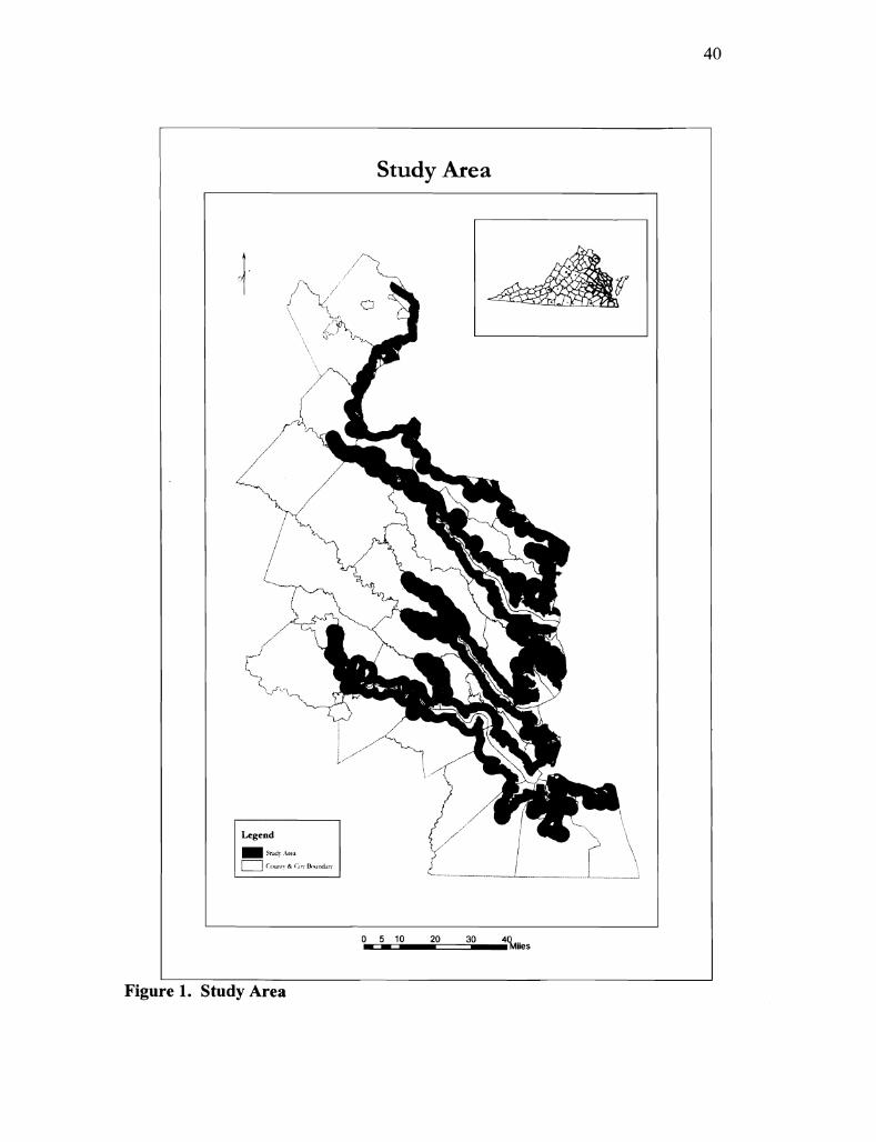
Figure 1 : Study area ........................................................................................................... 40
Figure 2: Study area regions .............................................................................................. 41
Figure 3: 2000 Impervious surface classification .............................................................. 42
Figure 4: Impervious surface suitability threshold ............................................................ 43
Figure 5. Bald eagle nests plotted against percent area bareland within a study area region .. ... . . .. .. .. .. ... .. .. .. ... .. .. ... .. .. .. ... .. .. . . .. . .. ... . .. .. ... ... . .. ... .. .. ... .. .. .. . . . .. .. .. .. .. .. .. . . .. .. .. . . . .. .. .. .. . . .. ..44
Figure 6. Bald eagle nests plotted against percent area agricultural land within a study area region . ... .. .. .. ... .. .. .. ... .... .. .. .. ... .. ... .. .. .. ... .. .. ... .. .. ... .. .. ... .. .. .. .. ... .. .. .. .. ... .. .. .. .. .. .. ... .. ... .. .. .. .. -45
Figure 7. Bald eagle nest plotted against percent area forested within a study area region. . ... .. . .. ... .. .. .. ... .. .. ... .. .. . .. .. ... .. .. ..-.. .. ... .. .. ... .. ... .. .. .. .. . .. .. ... .. .. .. ... ... .. .. .. .. .. .. .. ... . ... .. ... . .. .. ..46
Figure 8. Bald eagle nest plotted against distance to shoreline (meters) within a study area region ......................................................................................................................... 47
Figure 9. Bald eagle nest plotted against percent impervious surface within a study area region . .. .. .. .. ... .. .. .. ... .. .. ... .. . .. .. .. . .. .. .. . . .. .. .. .. ... ... .. ... .. .. .. .. ... .. ... .. .. .. ... .. .. .. ... .. .. .. . ... .. .. .. .. .. ... .. .. ... 49
Abstract
A GIs AND REMOTE SENSING BASED ANALYSIS OF IMPERVIOUS SURFACE INFLUENCES ON BALD EAGLE (HALIAEETUS LEUCOCEPHALUS) NEST
PRESENCE IN THE VIRGINIA PORTION OF THE CHESAPEAKE BAY
By Jennifer Ciminelli, M.S.
A Thesis submitted in partial fulfillment of the requirements for the degree of Master of Science, Environmental Studies at Virginia Commonwealth University.
Virginia Commonwealth University, 2006
Major Professor: Dr. Gregory C. Garman, Ph.D. Director, Center for Environmental Studies
GIs (Geographic Information Systems) and remote sensing techniques were
used to predict relationships between bald eagle nest presences and land type, distance
to land type and impervious surface cover area. Data plots revealed bald eagle nest
presence decreases in response to an increase in area of bareland; increases with an
increase in area of forested land; decreases with an increase in distance (m) to shoreline,
and decreases in response to an increase in area of impervious surfaces. Logistic
regression models identified impervious surfaces as an indicator for bald eagle nest
vi

vii
presence (P < 0.001). Chi-square analyses were used to develop a threshold model to
predict bald eagle nest presence in relation to percent impervious surface cover (6 DF,
value 45.0739, P < 0.0001). Three threshold levels were identified, 0 - 6% impervious
cover as sensitive, 7 - 23% as impacted, and > 24% as unsuitable. Unsuitable area
covered 17.82% of the total study area, impacted area covered 13.40%, and, sensitive
area covered 68.77%. The projected increase in population in the state of Virginia and
subsequent increase in impervious surfaces presents a challenge to the future viability of
the Virginia Chesapeake Bay bald eagle population. The threshold analysis identified
areas of prime conservation concern for bald eagle nest presence within the defined
study area. These areas provide the basis for a conservation management plan and for
further scientific study.
Key words: ESRIO ArcGIS, ESRIO ArcINFO, ESRIO ArcView 3.x, Bald eagle, Chesapeake Bay, Chi-square analysis, ERDASO Imagine, GIs, Geographic Information System, Haliaeetus leucocephalus, impervious surface, remote sensing, SASO System 8.x, Virginia, watershed management

INTRODUCTION
Prior to European settlement, the Chesapeake Bay area provided forested
shoreline habitat and ample prey for an estimated 3000 pairs of bald eagles (Haliaeetus
leucocephalus) (Fraser et al. 1996). In the early 1900s, bald eagle populations began to
decline due to hunting, persecution and habitat destruction (Stalmaster 1987, Fraser et
al. 1996). Environmental factors, such as the use of the pesticide DDT (dichloro-
diphenyl-trichloroethane), along with the effect of its "metabolites", DDE (dichloro-
diphenyl-dichloroethylene) and DDD (dichloro-diphenyl-dichloroethane), caused
eggshell thinning, which affected the reproductive success of bald eagles and population
numbers continued to decline during the 1900s (Stalmaster 1987, Watts 1999). In 1972,
DDT and other chemical pesticides were banned in the United States (Watts 1999). Up
to that point in time, bald eagles were legally protected under the Lacey Act, The
Migratory Bird Treaty Act and The Bald and Golden Eagle Act (Stalmaster 1987, Watts
1999). These acts were effective in protecting the species itself with prohibitions
against the sale, trade or hunting of the eagle, but it was not until the Endangered
Species Act of 1973, and the subsequent listing of the bald eagle as an endangered
species in 1978, that habitat protection was also afforded to the bald eagle. These
combined efforts helped contribute to the increase in bald eagle population numbers. In

2
2001, Virginia had 33 1 occupied territories and 3 13 active nests (Watts and Byrd,
Bald eagles choose nest locations in response to many factors, including prey
vulnerability (Hunt and Jenkins, 1992, Dzus and Gerrard, 1993), proximity to open
water, suitable nest and roost habitat and human disturbance (Stalmaster 1987,
Livingston et al. 1990, Buehler et al. 1994b, Chandler et al. 1995, Watts 1999). Nest
trees tend to be the largest trees in the stand, often large loblolly pines, typically found
in old growth forests, within one mile (1.6 km) of open water, preferably of a channel
width of 250 meters (Andrew and Mosher 1982, Stalmaster 1987, Watts 1999). In
Virginia, prime bald eagle habitat is found along the coast of the Chesapeake Bay and
it's tributaries.
The Chesapeake Bay Watershed, the largest estuary in North America, has an
area of 64,000 square miles providing habitat to thousands of aquatic and terrestrial
species of wildlife, and functioning as part of the Atlantic Migratory Bird Flyway
(Alliance for the Chesapeake Bay 2005, U.S FWS 2005). With 11,684 miles of
shoreline, the Bay provides optimal nesting habitat for bald eagles (Alliance for the
Chesapeake Bay 2005), supporting "the second largest breeding population.. .on the
east coast" (Therres et al. 1993). In addition to the ecological significance of the Bay,
the Chesapeake Bay shoreline is considered prime real estate for development.
With the impending removal of the bald eagle from the Endangered Species List
and the lack of established habitat conservation initiatives, critical habitat for the bald
eagle in the Chesapeake Bay Region is in danger of being irretrievably lost to human

3
development. Total population for the state of Virginia in 2000 was 7,078,515 and is
projected to be 8.5 million for the year 2025 (U.S. Census Bureau 1997,2005). The
Virginia Conservation Network predicts Virginia "will develop more land in the next 40
years than it has in the past 400 years" (VCN 2002). The increase in population will
place humans in direct competition with bald eagles for available land and resources.
As shoreline continues to be developed, it cannot be presumed that eagles will learn to
adapt to these human disturbances (Fraser et al. 1985, Buehler et al. 1991b, Therres et
al. 1993, Steidl and Anthony 1996).
Numerous studies have been conducted across the United States evaluating bald
eagle responses to human disturbances (Livingston et al. 1990, Grubb et al. 1992,
Therres et al. 1993, Watts et al. 1994, Steidl and Anthony 1996). There is a consistent
finding across the landscape that bald eagles exhibit a negative response to human
disturbance (Fraser et al. 1996), locating nests away from development to avoid human
interaction.
Bowennan et al. (1993) reported relationships between wintering bald eagle
perch tree selection and type of "potential human disturbance". The study found bald
eagles chose perch trees away from human disturbance, which is supported by Buehler
et al. (1991a, 1992) and Chandler et al.'s (1995) findings that bald eagle habitat
selection on the Chesapeake Bay was influenced by the combined effect of human
activity and perch tree availability. Human activity negatively affects bald eagle
distribution whether through the activity itself or the presence of the developed
4
landscape (Fraser et al. 1985, Brown and Stevens 1997, Buehler et al. 1991b, Steidl and
Anthony 2000).
Past studies conducted on eagle response to human activity have concentrated
on small population studies in a constrained area. These studies have quantified
specific parameters at fine details to better understand bald eagle behavior. The
difficulty in these studies is the application of the findings across a wide range of
landscapes, particularly as bald eagle behavior may be unique to specific populations
and can be difficult to quantify (Grubb et al. 1992, Steidl and Anthony 1996).
To evaluate bald eagle presence or absence in relation to human disturbance
over a large geographic area, a Geographic Information System (GIS) and remote
sensing based analysis was employed. The use of a large spatial area allows for a
coarser evaluation of bald eagle presence, providing results that can be applied across a
wider scale of habitat. Finer resolute studies concentrate on populations that may
exhibit similar intra-population characteristics, but may be unique from other eagle
populations. The coarser study combines populations across a wide spatial extent and
develops a comprehensive threshold evaluation.
A GIS is defined as "an organized collection of computer hardware, software,
geographic data, and personnel designed to efficiently capture, store, update,
manipulate, analyze, and display all forms of geographically referenced information"
(ESRI 1997). GIS and remote sensing techniques are becoming viable analytical tools
with which to assess urban growth with the use of impervious surfaces coverages as
indicators of human development (Pathan et al. 1993, Deguchi and Sugio 1994).
5
Impervious surface area has been a commonly used watershed management tool in the
assessment of watershed quality (Martin 2000, Zielinksi 2002). The increase in human
population and continued expansion into the landscape results in an increase in
impervious surfaces. The state of Virginia has experienced a 44.7% increase in
imperviousness from 1990 to 2000 (Chesapeake Bay Program 2004). It can be
extrapolated that impervious surfaces can serve as indicators of anthropogenic
influences on current habitat, and as measures of human population growth (Arnold et
al. 1996) and subsequent development and disturbance.
The continuing increase in human population and impending development
requires an assessment of current habitat for eagle nest presence (Buehler et al. 1991b,
199 1 c). Once these areas have been identified, concentrated studies can be performed
and specific management plans enacted to ensure bald eagle carrying capacity in the
Virginia portion of the Chesapeake Bay is not breached.
GIs and remote sensing techniques on classified Landsat TM scenes were used
to analyze eagle nest presence in response to land type and distance within the Virginia
portion of the Chesapeake Bay Watershed. The data were then further analyzed to
establish a threshold level of percent impervious area as an indicator of anthropogenic
influences and the effect on bald eagle nest presence. The use of thresholds will
establish parameters within which further studies can be concentrated to fully explore
the level of effect of human disturbance and development has on .the bald eagle.
The objectives of this study are to: (I) to examine the relationship between bald
eagle nest location and land type; (2) to examine the relationship between bald eagle

nest location and distance to defined land types; and (3) to predict percent area
impervious surface thresholds in relation to presence of bald eagle nests in the Virginia
portion of the Chesapeake Bay watershed. The null hypothesis of .the study is that there
is no relationship between impervious surfaces and bald eagle nest presence.
STUDY AREA
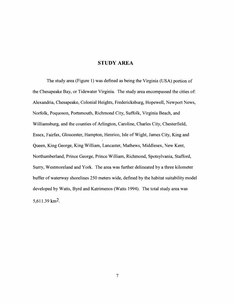
The study area (Figure 1) was defined as being the Virginia (USA) portion of
the Chesapeake Bay, or Tidewater Virginia. The study area encompassed the cities o f
Alexandria, Chesapeake, Colonial Heights, Fredericksburg, Hopewell, Newport News,
Norfolk, Poquoson, Portsmouth, Richmond City, Suffolk, Virginia Beach, and
Williamsburg, and the counties of Arlington, Caroline, Charles City, Chesterfield,
Essex, Fairfax, Gloucester, Hampton, Henrico, Isle of Wight, James City, King and
Queen, King George, King William, Lancaster, Mathews, Middlesex, New Kent,
Northumberland, Prince George, Prince William, Richmond, Spotsylvania, Stafford,
Surry, Westmoreland and York. The area was further delineated by a three kilometer
buffer of waterway shorelines 250 meters wide, defined by the habitat suitability model
developed by Watts, Byrd and Katrimenos (Watts 1994). The total study area was
5,611.39 km2.
METHODS
Dr. Mitchell Byrd and Dr. Bryan Watts of the Center for Conservation Biology
at William and Mary, in collaboration with the Virginia Department of Game and
Inland Fisheries (DGIF), conducted surveys of bald eagle nest locations in 2000 for the
entire state of Virginia. Surveys were conducted from an aircraft and recorded on
United States Geological Survey (USGS) topographic maps in the Universal Transverse
Mercator (UTM), Zone 18 North American Datum (NAD) 1927, in units of meters.
UTM is a coordinate system based on the Transverse Mercator projection where the
world is divided into sixty zones (ESRI 1997). The study area fell completely within
UTM Zone 18 of the UTM projection, which minimizes distortion of area and distance
and preserves shape and direction (ESRI 1997, ESRI 1994). Bald eagle nest location
data were obtained from the Center for Conservation Biology in DBASE IV (.dbf)
format. Coordinates were converted from .dbf format into a GIs point coverage using
the Create Feature Class from X, Y Table in ESRIO Arccatalog. The points were then
reprojected to UTM 18 NAD WGS84 projection in ESRIO ArcGIS, using the Project
command with datum transformation.
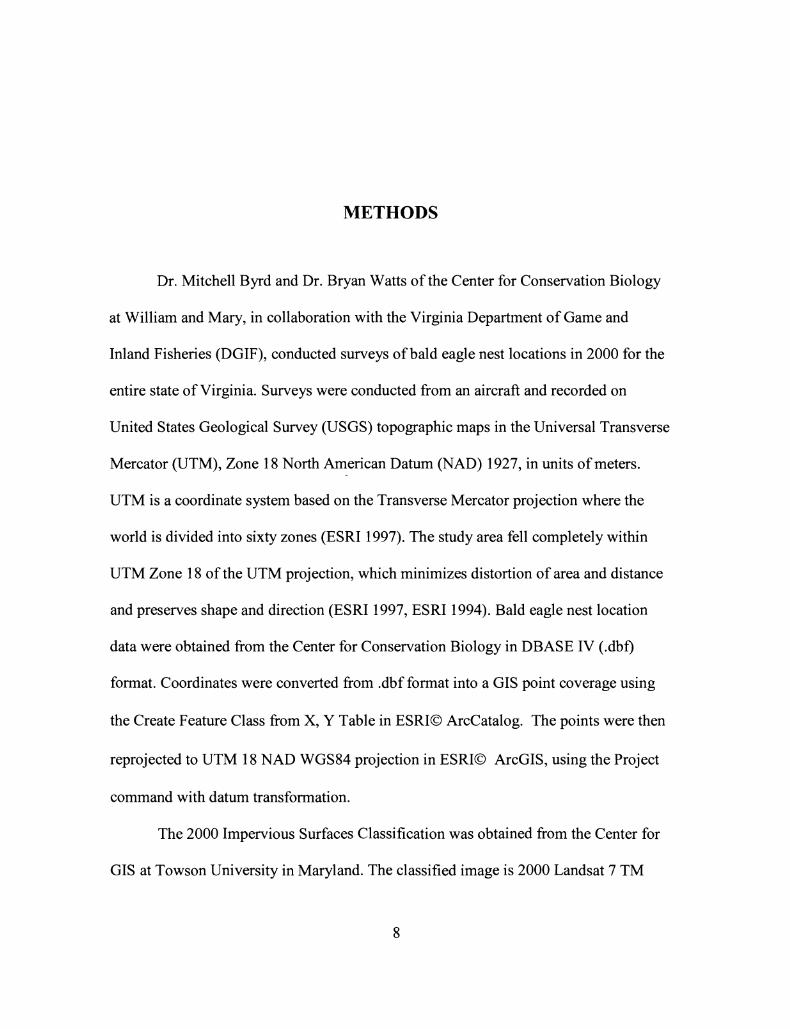
The 2000 Impervious Surfaces Classification was obtained from the Center for
GIs at Towson University in Maryland. The classified image is 2000 Landsat 7 TM

9
imagery and was tiled by county in .gis format. Available data for the study area were
imported to image form using the Imagine Import tool under the Import / Export menu
in ERDASO IMAGINE.
Raw Landsat ETM+ scenes 14/34 (path / row) and 15/33 were downloaded
from the Chesapeake Bay from Space Program image repository as individual bands for
Virginia Beach and the surrounding areas. These files were needed to fill in the missing
area in the classified 2000 data from the Chesapeake Bay from Space classification.
Bands one through five and band seven have a spatial resolution of 30 meters and are
useful in evaluating land use types (USGS 2004). The thermal IR band 6 has a coarser
resolution of 60 meters, and is generally used to assist in thermal mapping (USGS
2004). Band 6 was subset from each scene in Imagine using the Layerstack Utility, to
help decrease file size.
A supervised classification was used to process the spectral reflectance of the
images, based on decision rules that defined spectral reflectance values and their
associated land type. The goal of a supervised classification is to have the computer use
defined parameters to automatically categorize, or group, pixels into specific land
classes, based on the pixel reflectance values (Lillesand and Kiefer 1994). Spectral
reflectance values of individual pixels in an image are based on the "inherent spectral
reflectance and emittance properties" of the features (Lillesand and Kiefer 1994).
Land types for the classification scheme were defined as Impervious Surfaces,
Deciduous Forest, Water, Coniferous Forest, Bareland, Agricultural Lands, Cloud and
Beach (Table 3).

10
The impervious surfaces class consisted of areas defined as a road, parking lot or
airport, and residential development where pixels of high imperviousness were
interspersed with non-impervious pixels, such as residential areas where houses and
driveways were interspersed with gardens and yards. Cloud and beach signatures were
collected to ensure that these signatures would not misclassify as bareland or low
imperviousness.
Supervised classifications (Appendix B) were run on each Landsat scene, using
the Signature File created for each scene with the Maximum Likelihood Parametric
Rule. This rule assumes a normal distribution of the training data, and calculates the
probability that a pixel belongs to each class before assigning the pixel to the class with
the highest probability (ERDAS 2004, Lillesand and Kiefer 1994). This method is seen
as the "most accurate classifier in the ERDAS IMAGINE system" (ERDAS 2004,
Lillesand and Kiefer 1994). An accuracy assessment was run in Imagine, 35 points
were generate for each class for a total of 210 points. Points were generated based on a
stratified random sampling. DOQQ's were used as the ancillary data source for the
accuracy assessment.
The final scenes were recoded to standardize the classification. Recoding was
done in ESRIO ArcEdit and in the IMAGINE Raster Attributes Editor on the Viewer
Menu. Necessary scenes were exported from IMAGINE to grid format using the Import
1 Export function. The grid was converted to a polygon in ESRIO ArcINFO
workstation using the Gridpoly command. Weed tolerance was set to "0.02 inches
(0.0508 cm) or equivalent coverage units" which was calculated to be 0.0000508 meters
11
(ESRI 2004). Weed tolerance is the minimum distance between vertices for arcs that
are added to a coverage (ESRI 2004).
Grid codes were recalculated and saved in ArcEdit using the Select and
Calculate commands. The polygon was converted from a coverage to a grid using the
ArcGRID Polygrid command. The grid was then imported to an image to run the
mosaic in Imagine. The Impervious Surfaces Classification was recoded with the Raster
Attribute Editor to reflect the defined classification classes in IMAGINE.
All individual scenes were merged into one seamless image using the Mosaic
Tool under the IMAGINE Data Prep menu with the Overlay hnction and with the
output set to a common lookup table. Scenes that had cloud cover were overlaid with
scenes with no cloud cover, replacing most of the cloud cover with a classified area.
The mosaiced image was subset with an A01 (Area of Interest) in IMAGINE.
The A01 was considered "the first constraint of the final" land classification
model. The model was developed by Dr. Bryan Watts of the Center for Conservation
Biology at the College of William and Mary (Watts et al. 1994). The pre-defined
working area was developed in GIs by Dr. Watts using editing techniques in ESRIO
ArcView 3.2. Open water channels of at least 250 m wide were digitized into an arc
shapefile. The coverage was buffered at 3 km using the Buffer Tool in ArcGIS to
create the working area AOI. The A01 was then clipped to exclude large water bodies,
rivers and the Bay water. This A01 was used to subset the final classified images in
IMAGINE using Subset command under the Data Prep menu with the working area as
the input AOI. The final image was considered the study area. The final mosaiced
12
2000 classification was exported to a grid with the Export Utility in IMAGINE. The
grid was exported to an ArcINFO coverage in Arc using the Gridpoly command. The
polygon coverage was then exported to a personal geodatabase feature class in
Arccatalog to ensure the area values were automatically updated with any geographic
alteration during post processing. The conversion from grid to coverage to personal
geodatabase was necessary to retain topological integrity of the data and was done in
this order to utilize the best software tools for each conversion. Topological integrity
deals with the spatial relationships of each piece of data to another, and to the associated
attribute information (ESRI 2004, ESRI 2002).
Post processing on the classification was done in the ESRIO ArcMap editing
environment. Digital Orthophoto Quarter Quadrangles (DOQQ) were used to classify
the polygon according to land use based on the defined classification scheme. A Union
was run in ArcGIS with the classified study area and the DOQQ grid as the input layers.
This was done to break the study area into regions for regression and Chi-Square
analyses. The output feature class was called study area regions (Figure 2). The
DOQQ grid represented regions within the study area. The region area boundaries were
3 ?h minute USGS quarter quadrangle. The feature class generated by the Union was
exported to a MicrosoftO Access database for statistical work.
To determine the distance from each land type to the closest Eagle nest, the
2000 classified grids were converted to polygon ArcINFO coverages. An AML script
was generated and executed to export each land type (by grid code value) into a
separate coverage. The Near command was then used to calculate the distance from

13
individual Eagle nest points to the nearest impervious land type, nearest deciduous
forest, shoreline, nearest coniferous forest, nearest bare land and nearest agricultural
land types. The output of the Near command was stored in the ArcINFO Eagle point
attribute table (.pat), which was exported into Excel.
The Select by Location function was used in ArcMap to identify the total
number of Eagle nests occurring within the study area. Eagle nests with the center
located within the study area were selected for analyses. A total of 210 Eagle nests
were within the study area. The Select by Location tool in ArcMap was used to
calculate numbers of Eagle nests occurring in each study area regions.
Two queries were run on the study area region feature class in Access to
generate a table with the grid code number (representing land type), the sum of the total
area of each unique quarter quad, the total area for each unique grid code within the
specific quarter quad region, the total area of the quarter quad and the percent area of
the study area. The percent area of a grid code was calculated by dividing the total area
of a grid code by the sum the total area of all polygons within a quarter quad region
study area with grid code > 0.
Study areas that were calculated to be less than ten percent of the total study
area were considered fragment areas. A Create Table Query was used in Access to
identify these study areas and were removed from the final regression database.
The SASO System for Windows Version 8 was used for statistical analyses.
Data were grouped according to defined statistical goals. Univariate statistics were run
to test for normality using the Proc Univariate command. Correlations were run to test
14
for interactions. Logistic regressions were run on the data in SAS using the Proc
Logistic command. Various models were tested with percent area of land type, number
of Eagle nests, distance from Eagle nest to each land type and shoreline and all
interaction terms. Stepwise selection was run on the model.
Eagle nest and percent area impervious surfaces were evaluated using Chi-
Square analyses using Proc Freq in SAS. Eagle nest data were grouped into four
categories; 0 for zero nests, 1 for one nest, 2 for two nests and 3 for greater or equal to
three nests. Percent impervious area was grouped into various combinations based on a
Watershed Vulnerability Analysis conducted by the Center for Watershed Protection.
Validation was run on the threshold levels with 914 nest locations surveyed
from 2001 to 2004 in ArcMap. Nest code is the unique identifier assigned to and
associated with each particular Eagle nest surveyed. Validation nests were overlaid on
the threshold grid to assess what threshold the nests were found to be present.

RESULTS
Landscape Characteristics
The 2000 Impervious Surfaces Classification was obtained from the Center for
GIs at Towson University in Maryland. The overall classification accuracy for the
2000 image was 85% (per communication with David Sides of Towson University, Fall
2002).
Landsat TM scenes 14/34 and 15/33, downloaded to supplement missing areas in the
2000 classification, had a signature separability for scene 14/34 of 1998, and 2000 for
scene 15/33. Overall classification accuracy for the VA Beach area was 63.3% with
Overall Kappa Statistics = 0.4176 and an impervious surface Kappa Statistic = 0.7141.
Study area size was equal to approximately 38 square kilometers (14.67 square
miles). Total area evaluated for the study was 5,6 1 1.39 square kilometers (2,166.56
square miles). Land type area in the study area totaled 2.09 % bareland, 4.86% inland
water, 13.12% impervious surface, 18.64% coniferous forest, 26.15% agricultural and
35.14% deciduous forest (Table 1).
Eagle Nest Location Results
Average distances (meters) were calculated from eagle nest point to nearest land
type and range from a minimum to maximum distance of 1.34 to 1 1 19.77 m to nearest
deciduous land type, 1.19 to 556.70 m to nearest coniferous land type, 1.19 to 7772.71
15

16
m to nearest agricultural land, 21.90 to 2880.52 m to the shoreline, 40.72 to 1914.13 m
to nearest impervious surface, and 61.95 to 4434.65 m to nearest bare land (Table 2).
Exploratory statistics indicate a negative correlation between number of eagle nests and
percent impervious surface area (-0.32077, p < .0001). Data plots revealed bald eagle
nest presence decreases in response to an increase in bareland (Figure 5); increases with
an increase in forested land (Figure 7); decreases with an increase in distance to
shoreline (Figure 8), and, decreases in response to an increase in impervious surfaces
(Figure 9).
Logistic regression yielded significant parameters at p < .05 (Table 4) for percent area
impervious, deciduous forest, bareland, agricultural land; distance from eagle nest to:
agricultural land, bareland, coniferous forest, deciduous forest, impervious land and
shoreline; interactions percent impervious and distance from eagle nest to: agricultural
land, bareland, coniferous forest, deciduous forest, impervious and shoreline;
interactions percent deciduous forest and distance from eagle nest to: agricultural land,
bareland, coniferous forest, deciduous forest, impervious land and shoreline;
interactions percent inland water and distance from eagle nest to: agricultural land,
bareland, coniferous forest, deciduous forest, impervious land and shoreline;
interactions percent coniferous forest and distance from eagle nest to agricultural land,
bareland, coniferous forest, deciduous forest, impervious land, and shoreline;
interactions percent bareland and distance from eagle nest to: agricultural land,
bareland, coniferous forest, impervious land and shoreline; and, interactions agricultural
land and distance from eagle nest to: agricultural land, bareland, coniferous forest and

17
impervious land. When percent area coniferous forest and deciduous forest were
combined, the parameter tested significant at p < .0001 with a percent concordant of
64.0.
Logistic regression for all land types (forested not combined) run with Stepwise
Selection at p < .25 yielded six significant parameters and one interaction term,
including the percent area impervious, distance from eagle nest to agricultural land,
distance to bareland, distance to coniferous forest, distance to impervious land, distance
to shoreline and the interaction term percent area impervious and distance to coniferous
land. Overall percent concordant was 91.1 %, indicating the model predicted the
presence of an eagle nest 9 1.1 % of the time.
Logistic regression for land types with deciduous and coniferous forest
combined run with Stepwise Selection at p < .25 yielded similar results: percent area
impervious, distance from eagle nest to agricultural land, distance to bareland, distance
to forest, distance to impervious land, distance to shoreline; and, the interaction terms
percent area impervious and distance to bareland and percent area impervious and
distance to impervious land.
Parameter estimates indicated positive and negative relationships for the logistic
regression formula predicting eagle nest presence; however, results of the full model
indicated multicollinear data.
Logistic regression results for the model eagle nest presence = percent
impervious surfaces (p < .0001 and percent concordant = 65.7) indicated a strong
relationship with which to evaluate threshold effects.
Impervious Thresholds
Chi-square tests run on eagle nest presence and suitability groups resulted in
percent area of impervious surface groupings where 0 - 6% impervious surface area
was classified with a suitability rating of 2 (sensitive area), 7 - 23% impervious surface
area was classified with a suitability rating of 1 (impacted), and > 24% impervious
surface area was classified with a suitability rating of 0 (not suitable) for bald eagle nest
presence (Table 5). Chi-square tests (6 DF, value 45.0739) were significant at p <
.0001 (Table 6).
Of the total study area, unsuitable area constituted 17.82%, impacted area constituted
13.40%, and, sensitive area constituted 68.77% (Figure 4, Table 7).
There were a total of 284 study areas within the region. Of the 284 areas, 55
were classed in suitability group 0,37 were classed in suitability group 1 and 192 were
classed in suitability group 2 (Appendix A). Chi-Square tests results (Table 6) indicate
52 occurrences where 0 eagle nests are present in suitability group 0, 18 occurrences in
suitability group 1, and 88 occurrences in suitability group 2; 2 occurrences where 1
eagle nest presence occurs in suitability group 0, 13 occurrences in suitability group 1,
and 53 occurrences in suitability group 2; 1 occurrence where 2 eagle nests present
occurs in suitability group 0 ,5 occurrences in suitability group 1, and 33 occurrences
suitability group 2; and, 0 occurrences where 3 or more eagle nests present occurs in
suitability group 0, 1 occurrence in suitability group 1, and 18 occurrences in suitability
group 2.

19
Threshold Test
Threshold tests yielded a total of 22 nests present in suitability group 0. Of the
22 nests, 12 were unique nests (several nests surveyed were present multiple years).
1 15 nests were present in suitability group 1, with 70 distinct nest codes; and 777 nests
were present in suitability group 2 with 432 distinct nest codes.
Suitability group 0 (Impaired 1 Not Suitable) had 2% of the total nests present,
suitability group 1 (Impacted) had 13% present and suitability 2 (Sensitive) had 85% of
total nests present.

DISCUSSION
Bald eagles choose nest habitat comprised of forest stands situated close to
shoreline (Stalmaster 1 987, Livingston et al. 1 990, Buehler et al. 1 992, Watts 1 994 et
al., Chandler et al. 1995). The location of the nest, while strongly influenced by habitat
types is also affected by proximity to human activity and development. The results of
this study indicate there is a relationship between bald eagle nest presence and
impervious surfaces, measured as human activity and development. Bald eagle nest
presence was affected at three threshold levels of percent area of impervious surface.
Bald eagles must have the appropriate habitat available to support their perch,
nest and prey requirements. This analysis indicates that bald eagle nest presence is not
only affected by distance from nest to shoreline, but also the amount of impervious
surfaces, deciduous forest, bareland, and agricultural land.
Land Type Area and Distance
In evaluating the area of specific land types present and the effect on eagle nest
presence, coniferous forests did not have a significant impact. Combining deciduous
and coniferous forest land types into a forested type proved significant. Results from
this study show an increase in bald eagle nest presence with an increase in forested land.
A possible explanation for the significance of the combined forested classes and non-
significance of coniferous forests may be the 25 meter resolution of the Landsat TM
2 0

2 1
scenes used for the classification. At this resolution, mixed forest stands of coniferous
and deciduous forest may be classed according to the dominant type found in a pixel
area. Because this study dealt with a coarser resolution of observation, deciduous and
coniferous forests can be combined into one forested class. Another explanation may
be that eagles are not showing a preference for forest types as much as a preference for
suitable nest and perch trees. Bowerman et al. (1 993) reported finding no distinct
difference between perch use of coniferous versus deciduous tree type for wintering
adult eagles.
Results indicate bald eagle nest presence decreased in response to an increase in
area of bareland. Eagles may nest close to bareland for flight take off, but when a
certain level of buffer is not available, it exposes eagles to human activity and
disturbance causing eagle nest abandonment (Grubb et al. 1992, Therres et al. 1993,
Steidl and Anthony 2000, Fernandez-Juricic and Schroeder 2003). Eagles may choose
forested type next to agricultural lands instead of bareland as the agricultural landscape
may provide the preferred flight path without the human disturbance element (Figure 6).
In addition, bareland does not provide the nest substrate or habitat preference for bald
eagle nest presence.
Presence of bald eagle's nests decreases with an increase in distance to
shoreline. Bald eagles avoid development and typically nest within one to two
kilometers of shoreline (Watts et al. 1994). The Bay provides an optimal prey base for
the bald eagle, which feed almost exclusively on fish along the Bay shoreline (Abbott
1978).

Impervious surfaces have a strong negative effect on the presence of bald eagle
nests. Bald eagles exhibit negative responses to human development avoiding
developed shoreline for perch habitat and foraging use and do not appear to habituate to
human disturbance (Therres et al. 1993, Watts et al. 1994, Fraser et al. 1985, Buehler et
al. 199 1 a, Buehler et al. 199 1 b). The effect of human disturbance on eagles is difficult
to quantify and may be manifested in various ways. Human activity may startle eagles,
particularly dangerous during nesting which may cause nest abandonment (Therres et
al. 1993). Residential and commercial development destroys and fragments habitat
buffer areas increasing exposure to human activity.
The full model test of all significant parameters yielded significant results, but
the models were multicollinear (Kleinbaum and Klein 2002). When one independent
land type increased, another independent land type would be affected making a full
model based on land type and distance to land type ineffective. Based on this analysis,
impervious surfaces were the best parameter to develop a model to predict bald eagle
nest presence.
Impervious Surfaces Thresholds
It can be presumed that as a population, species will respond to a specific
parameter up to a particular threshold, after that particular threshold is breached, the
habitat can be considered unsuitable or degraded at such a level to cause a population
response (Van Horne 1991). Thompson and McGarigal(2002) evaluated "scale-
dependant relationships in wildlife habitat" and found critical threshold values for
"eagles' response to shoreline development" indicating not only a relationship, but the

2 3
effect of using threshold analyses at particular scales of study. To develop a threshold
for bald eagles that would be applicable across the Chesapeake Bay Watershed, a larger
spatial extent was evaluated. Evaluating individual nest areas or groups of small nest
areas may not provide enough inter-species rich data to establish the threshold
relationship.
The results of this analysis indicate that impervious surface thresholds for bald
eagle nest presence along the Virginia portion of the Chesapeake Bay do exist. Bald
eagles presence can be grouped into three response levels: 0 - 6% impervious surface
area as sensitive habitat (suitability rating of 2), 7 - 23% impervious surface area as
impacted habitat (suitability rating of I), and L 24% impervious surface area classified
as unsuitable (suitability rating of 0). The threshold results are closely tied to the Center
for Watershed Protection's Watershed Vulnerability Analysis (Zielinski 2002) that
measured stream quality based on percent impervious surface within a subwatershed.
The Vulnerability Analysis categorized a subwatershed area with 0 to 10% impervious
cover as a Sensitive Stream with "excellent habitat structure, good to excellent water
quality, and diverse communities of both fish and aquatic insects" (Zielinski 2002). A
subwatershed with 11 to 25% impervious cover is categorized as an Impacted Stream,
showing signs of habitat "degradation due to watershed urbanization"; and, a
subwatershed that exceeds 25% impervious cover is categorized as a Non-Supporting
Stream (Zielinski 2002).
Ecologically, the health of a watershed represents the ecological integrity of an area to
support species richness.

24
In areas classed as sensitive in this study, the ecological integrity exists to
support bald eagle presence. The area has the habitat to support bald eagle roosting and
nest preference, and prey requirements. In addition, these areas have low human
disturbance effects, seen as low impervious surface area.
Impacted habitat supports bald eagle presence, but the ecological integrity of the area is
negatively affected. The area's available eagle habitat is decreasing due to human
development. These areas are also prone to human activity disturbance effects. This
particular threshold represents time sensitive areas for habitat conservation.
Unsuitable habitat represents areas that are not suitable for eagle nest presence.
The high impervious surface cover in these areas indicates a high human disturbance
level. These areas do not support the nesting and 1 or foraging habitat needed for eagle
nest presence.
While all suitable land for eagle presence represents important conservation
areas, the impacted threshold areas are in particular danger of becoming lost to
development, and subsequently unsuitable. These areas represent time-sensitive
conservation areas, as the area may cross the threshold to unsuitable in less time than a
suitable area. Identifying these particular areas alerts scientists and local land planners
to the sensitivity of these areas and the danger associated with introducing development
in the area.

MANAGEMENT IMPLICATIONS
The Endangered Species Act has given the bald eagle the habitat conservation
measures necessary to ensure eagle habitat conservation and protection. With the
impending removal of the species from Threatened status, management practices must
be adapted at a local scale to ensure habitat and species conservation.
Long term management plans need to be developed in response to current eagle
habitat and existing development pressures. Watts (1999) has indicated that a "20%
increase in the human population" for -the year 2020 "will result in a 60% increase in
developed land". Bald eagles and humans are in direct competition for habitat. Watts
has predicted that the bald eagle population in Virginia will reach carrying capacity at
550 pairs (Springston 2005). At that point, the eagle population will begin to decline.
Species specific management for the bald eagle helped bring the eagle back from its
endangered status. However, there is a need to develop a coarser tool with which to
manage the ecological integrity of an area to support many species.
Local governments are responsible for land use planning with open space
management, an existing component of land use planning. These requirements deal
with the amount of impervious surface allowed in a defined area (i.e. lot area). Taking
a watershed management approach to land use planning, with the incorporation of

2 6
species specific thresholds will provide planners with an effective sustainable growth
plan for their locality and for the bald eagle.
The threshold analysis identified areas of prime conservation concern for bald
eagle nest presence within the defined study area. These areas provide the basis for a
conservation management plan and for further scientific study. The particular threshold
level areas should be further analyzed to quantify what effect(s) are causing the breach
of an area that once acted to support bald eagle nest presence to become unsuitable. In
understanding these cause and effect relationships change can be made to support smart
growth, conservation goals, and the ecological integrity of our environment.

Literature Cited
Abbott, J.M. 1978. Chesapeake Bay Bald Eagles. Delaware Conservationist 22: 3-9.
Anthony, R. C., R. W. Frenzel, F. B. Isaacs, and M. G. Garrett. 1994. Probable causes of nesting failures in Oregon's bald eagle population. Wildlife Society Bulletin 22: 576-582.
Arnold C. L. and C. J. Gibbons. 1996. Impervious Surface Coverage The Emergence of a Key Environmental Indicator. Journal of the American Planning Association 62(2): 243 - 258.
Bowerman W. W., IV, T. G. Grubb, A. J. Bath, J. P. Giesy, Jr., G. A. Dawson, and R. K. Ennis. 1993. Population composition and perching habitat of wintering bald eagles, Haliaeetus leucocephalus, in northcentral Michigan. The Canadian Field-Naturalist 107(3):273-278.
Brown B. T. and L. E. Stevens. 1997. Winter bald eagle distribution is inversely correlated with human activity along the Colorado River, Arizona. Journal of Raptor Research. 3 l(1): 7-10.
Buehler, D. A., T. J. Mersmann, J. D Fraser, and J. K. D. Seegar. 1991a. Nonbreeding Bald Eagle Communal and Solitary Roosting Behavior and Roost Habitat on the Northern Chesapeake Bay. Journal of Wildlife Management 55 (2): 273 - 28 1.
-------- -------- -------- -------- , , , . 1991b. Effects of human activity on bald eagle distribution on the Northern Chesapeake Bay. Journal of Wildlife Management 55(2): 282-290.

- - - - - - - - , J. D. Fraser, J. K. Seegar, G. D. Therres, and M. A. Byrd. 1991c. Survival rates and population dynamics of bald eagles on Chesapeake Bay. Journal of Wildlife Management 55(4): 608-61 3.
-------- , S. K. Chandler, T. J. Mersmann, J. D. Fraser,. and J. K. D. Seegar. 1992. Nonbreeding Bald Eagle Perch Habitat on the Northern Chesapeake Bay. Wilson Bulletin 104(3): 540 - 545.
Chandler S. K., J. D. Fraser, D. A. Buehler, and J. K. D. Seegar. 1995. The perch tree and shoreline development as predictors of bald eagle distribution on Chesapeake Bay. Journal of Wildlife Management. 59(2): 325-332.
Deguchi C. and S. Sugio. 1994. Estimations for Percentage of Impervious Area by the Use of Satellite Remote Sensing Imagery. Water Science Technology 29(102): 135-144.
Dzus, E. H. and J. M. Gerrard. 1993. Factors influencing bald eagle densities in Northcentral Saskatchewan. Journal of Wildlife Management 57(4): 77 1-778.
ERDAS 2004. Erdas Field Guide, Seventh Edition.
ESRI, 1994. Map Projections; Georeferencing Spatial Data.
ESRI, 1997. Understanding GIs; The ARCINFO Method.
ESRI 2004. ARCIINFO Help.
Fernindez-Juricic, E., and N. Schroeder. 2003. Do variations in scanning behavior affect tolerance to human disturbance? Applied Animal Behaviour Science 84: 2 19- 234.

Fraser J. D., D. Frenzel, and J. E. Mathisen. 1985. The impact of human activities on breeding bald eagles in North-Central Minnesota. Journal of Wildlife Management 49(3): 585-592.
- - - - - - - - , S. K. Chandler, D. A. Buehler, and J. K. D. Seegar. 1996. The decline, recovery and future of the bald eagle population of the Chesapeake Bay, U.S.A. Pages 18 1-1 87 in Meyburg, B. U. and R. D. Chancellor,eds. Eagle Studies.
Grubb T. G., W. W. Bowerman, J. P. Giesy and G. A. Dawson. 1992. Responses of bald eagles, Haliaeetus leucocephalus, to human activities in northcentral Michigan. The Canadian Field-Naturalist 106(4): 443-453.
Hunt, W. G., and J. M. Jenkins. 1992. Foraging Ecology of Bald Eagles on a Regulated River. Journal of Raptor Research 26(4): 243 - 256.
Kleinbaum, D. G and M. Klein. 2002. Logistic Regression: A Self-learning Text, Second Edition. Springer-Verlag, New York, NY.
Lillesand, T. M. and R. W. Kifer. 1994. Remote Sensing and Image Interpretation, Third Edition. John Wiley and Sons, Inc., New York, NY.
Livingston, S. A., C. S. Todd, W. B. Krohn, and R. B. Owen, Jr. 1990. Habitat models for nesting bald eagles in Maine. Journal of Wildlife Management 54(4): 644-653.
Martin E. W. 2000. Impervious Surface Area Spectral Mixture Analysis. The Community and Environmental Spatial Analysis Center. <www.commonsvace.org>. Accessed 2005 August.
Pathan, S. K., Sastry, S.V., et al. 1993. "Urban Growth Trend Analysis using GIs Technique - A Case Study of the Bombay Metropolitan Region", International Journal of Remote Sensing, Vol. 14, 1993, pp. 3 169-3 179.
Springston, R. 2005. Eagles thriving, but space limited. Richmond Times Dispatch. Pp. B1, B5.
30
Stalmaster, M. B. 1987. The Bald Eagle. Universe Books, New York, NY. 227pp.
Steidl, R. J. and R. G. Anthony. 1996. Responses of Bald Eagles to Human Activity During the Summer in Interior Alaska. Ecological Application 6(2): 428 - 491.
-------- -------- 7 . 2000. Experimental Effects of Human Activity on Breeding Bald
Eagles. Ecological Applications 10: 258 - 276.
Therres G. D., M. A. Byrd, and D. S. Bradshaw. 1993. Effects of development on nesting bald eagles: Case studies from Chesapeake Bay. Trans. Sth North American Wildlife and Natural Resource Conference, 62-69.
Thompson, C. M., and K. McGarigal. 2002. The influence of research scale on bald eagle habitat selection along the lower Hudson River, New York (USA). Landscape Ecology: 569-586.
USGS, 2004. Landsat Thematic Mapper Data (TM). USGS homepage. <http:lledc.usgs.govlguidesllandsat tm.html/#tml4>. Accessed 2005 Aug 8.
Watts, B.D. and M. A. Byrd 2002. Virginia bald eagle nest and productivity survey: Year 2002 report. Center for Conservation Biology Technical Report Series, CCBTR- 02-03. College of William and Mary, Williarnsburg, VA.
-------- . 1999. Removal of the Chesapeake Bay bald eagle from the federal list of threatened and endangered species: Context and Consequences. White Paper Series. The Center for Conservation Biology College of William and Mary. 16pp.
-------- , M. A. Byrd, and G. E. Kratimenos. 1994. Production and implementation of a habitat suitability model for breeding bald eagles in the lower Chesapeake Bay (Model Construction .through Habitat Mapping). Final Report, Virginia Department of Game and Inland Fisheries, 5 lpp.
Van Horne, B. and J. A. Wiens. 1991. Forest bird habitat suitability models and the development of general habitat models. Fish and Wildlife Research 8. 1-3 lpp.

Zielinski J. 2002. Watershed Vulnerability Analysis. Center for Watershed Protection. Ellicott City, MD.

32 Table 1. Percent area of land tv~es .
Y 1
BARELAND WATER IMPERVIOUS CONIFEROUS AG DECIDUOUS (INLAND)

Table 2. Average distance (meters) from Bald Eagle nest to land type. LAND DECIDUOUS CONIFEROUS AG SHORELINE IMPERVIOUS BARELAND TYPE MINIMUM 1.3440 1.1880 1.1880 21.898 40.7190 61.9460 MAXIMUM 1 1 19.7650 556.7015 772.71 2880.5166 1914.1270 4434.6520

Table 3. Classification Scheme and Grid Code
CLASS GRID CODE Impervious Surfaces 1 Deciduous Forest Water Coniferous Forest Bareland Agricultural Lands Cloud Beach
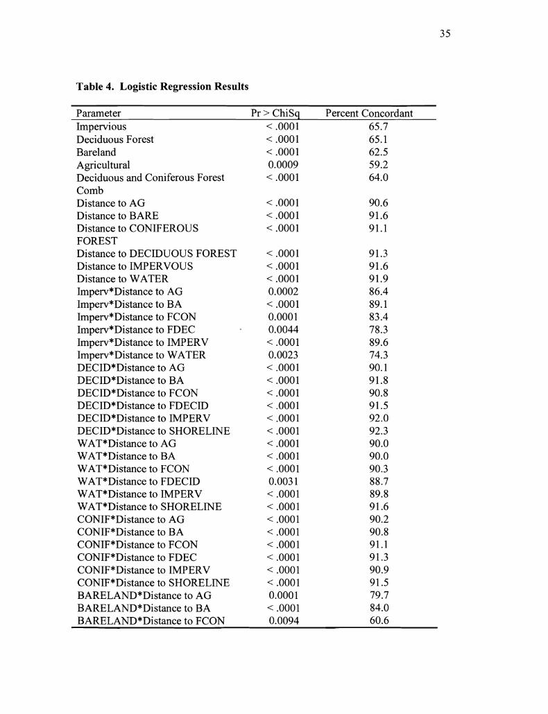
Table 4. Logistic Regression Results
Parameter Impervious Deciduous Forest Bareland Agricultural Deciduous and Coniferous Forest Comb Distance to AG Distance to BARE Distance to CONIFEROUS FOREST Distance to DECIDUOUS FOREST Distance to IMPERVOUS Distance to WATER Imperv*Distance to AG Imperv*Distance to BA Imperv*Distance to FCON Imperv*Distance to FDEC Imperv*Distance to IMPERV Imperv*Distance to WATER DECID*Distance to AG DECID*Distance to BA DECID*Distance to FCON DECID*Distance to FDECID DECID*Distance to IMPERV DECID*Distance to SHORELINE WAT*Distance to AG WAT*Distance to BA WAT*Distance to FCON WAT*Distance to FDECID WAT*Distance to IMPERV WAT*Distance to SHORELINE CONIF*Distance to AG CONIF*Distance to BA CONIF*Distance to FCON CONIF*Distance to FDEC CONIF*Distance to IMPERV CONIF*Distance to SHORELINE BARELAND*Distance to AG BARELAND*Distance to BA BARELAND*Distance to FCON
Pr > ChiSq < .0001 < .0001 < .0001 0.0009 < .0001
Percent Concordant 65.7 65.1 62.5 59.2 64.0
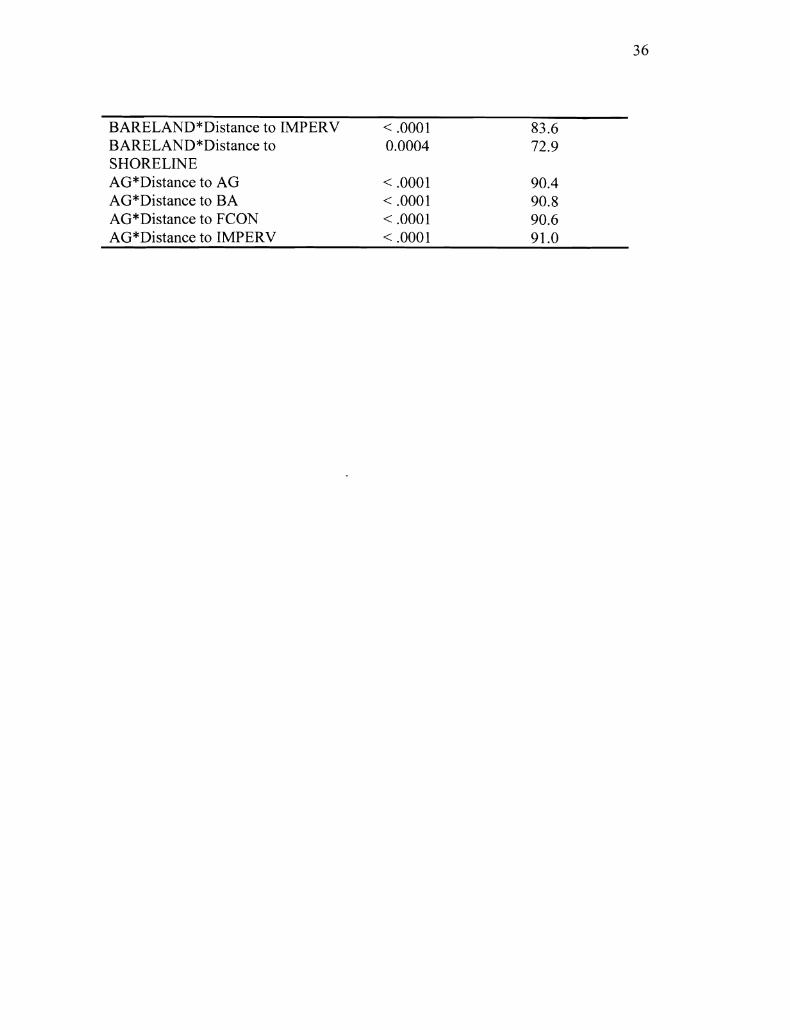
BARELAND*Distance to IMPERV < .0001 83.6 BARELAND*Distance to 0.0004 72.9 SHORELINE AG*Distance to AG < .0001 90.4 AG*Distance to BA < .0001 90.8 AG*Distance to FCON < .0001 90.6 AG*Distance to IMPERV < .0001 91 .O

Table 5. Suitability Ranks for Threshold Levels for Impervious Surfaces
PERCENT AREA SUITABILITY RANK DESCRIPTION IMPERVIOUS SURFACE
0 - 6% 2 Sensitive area. 7 - 23% 1 Impacted area. > 24% 0 Impaired 1 Not Suitable.

Table 6. Chi-Square Results

Table 7. Total area (meters and %) of suitability rankings.
Ranking Suitability 0 Suitabilitv 1 Suitabilitv 2 Total Area 988552900.36 743 172050.94 3 8 14220446.18 Percent of Study 17.82 13.40 68.77 Area
Study Area
I
Figure 1. Study Area

Figure 2. Study Area Regions

Figure
2000 Impervious Surf'ace Classification
3. 2000 Impervious Surface Classification

2000 Suitability Classification
lmpvrrd / k r Cuvhlr
Savrs Cww lyBoundary MDP 0 5 10 20 30 %iles 2000 1- Swhg cksmdml Cmf6rWGIS J m l h h x Q '
Figure 4. Impervious Surface Suitability Threshold

Figure 5. Bald eagle nests plotted against percent area bareland within a study area region. One triangle represents one bald eagle nest, triangles may be stacked representing one or more eagle nest.
Eagle Nest vs. Percent Bareland 5 1
Eagle Nests
41Y A
3 i w 1
2.1- AA
1 i A A A
00 A1 A I A I 0 5 - 10 15 20 25
Percent Bareland

Figure 6. Bald eagle nests plotted against percent area agricultural land within a study area region. One triangle represents one bald eagle nest, triangles may be stacked representing one or more eagle nest.
Eagle Nests vs Percent Area Agriculture 5-
4--
3 -
Eagle Nests
A
A
A A M A
A A A A m A m A M A U A A A
1 - - A A m " I r Y Y Y A Y A A
00 - A A A
0 -2 0 4 0 60 80
Percent Area Agriculture

Eagle Nests vs. Percent Area Forested
4--
3--
2--
1--
0 0 20 40 60 80 100
Percent Area Forested
Figure 7. Bald eagle nests plotted against percent area forested within a study area region. One triangle represents one bald eagle nest, triangles may be stacked representing one or more eagle nest.

Figure 8. Bald eagle nest plotted against distance to shoreline (meters) within a study area region. One triangle represents one bald eagle nest, triangles may be stacked representing one or more eagle nest.
Eagle Nest vs. Distance to Shoreline 5-
4--
3--
Eagle Nests
OA
A
A A m A A A
2-Y.U"Y"LIA A A
11- Y I Y I A A A A Y
I I I I 0 500 1000 1500 2000
Distance to Shoreline (meters)

Figure 9. Bald eagle nest plotted against percent impervious surface within a study area region. One triangle represents one bald eagle nest, triangles may be stacked representing one or more eagle nest.
Eagle Nests vs. Percent Impervious Surface
Eagle Nests
5-A
4 d y I
3iWA A
2 i W A A A A A
11-A A
0 I 0 20 - 40 60 80 100
Percent Impervious Surface

APPENDIX A. Suitability Ranking of Study Area
QNAME SUITABILITY ALEXANDRIA NE 0 ALEXANDRIA NW 0 ALEXANDRIA SE 0 ALEXANDRIA SW 0 BOWERS HILL NE 0 BOWERS HILL SE 0 CAPE HENRY SE 0 CAPE HENRY SW 0 CHESTER NE 0 COLONIAL BEACH NORTH SW 0 DREWRYS BLUFF NE 0 DREWRYS BLUFF NW 0 DREWRYS BLUFF SW 0 FALLS CHURCH SE 0 FENTRESS NW 0 FREDERICKSBURG NW 0 FREDERICKSBURG SW 0 HAMPTON NW 0 HAMPTON SE 0 HAMPTON SW 0 HOPEWELL SE 0 KEMPSVILLE NE 0 KEMPSVILLE NW 0 KEMPSVILLE SW 0 LITTLE CREEK SE 0 LITTLE CREEK SW 0 MOUNT VERNON NE 0 MOUNT VERNON NW 0 MULBERRY ISLAND NE 0 NEWPORT NEWS NORTH NE 0 NEWPORT NEWS NORTH NW 0 NEWPORT NEWS NORTH SE 0 NEWPORT NEWS NORTH SW 0 NEWPORT NEWS SOUTH NE 0 NEWPORT NEWS SOUTH NW 0 NEWPORT NEWS SOUTH SE 0 NORFOLK NORTH NE 0 NORFOLK NORTH SE 0 NORFOLK NORTH SW 0

50
NORFOLK SOUTH NE 0 NORFOLK SOUTH NW 0 NORFOLK SOUTH SE 0 NORFOLK SOUTH SW 0 NORTH VIRGINIA BEACH SW 0 OCCOQUAN SE 0 PRINCESS ANNE NE 0 PRINCESS ANNE NW 0 QUANTICO NW 0 RICHMOND SE 0 RICHMOND SW 0 SMITHFIELD NE 0 VIRGINIA BEACH NW 0 WASHINGTON WEST SW 0 YORKTOWN SE 0 YORKTOWN SW 0 BENNS CHURCH NW 1 BOWERS HILL NW 1 CHUCKATUCK NE 1 CHUCKATUCK NW 1 CLAY BANK SE 1 CLAY BANK SW 1 COLONIAL BEACH SOUTH NW 1 DAHLGREN NE 1 DEEP CREEK NE 1 DELTAVILLE SW 1 DREWRYS BLUFF SE 1 FORT BELVOIR NE 1 FORT BELVOIR NW 1 FORT BELVOIR SW 1 FREDERICKSBURG SE 1 HAMPTON NE 1 HOG ISLAND NE 1 HOPEWELL NW 1 HOPEWELL SW 1 MORATTICO SE 1 NEWPORT NEWS SOUTH SW 1 NORGE SE 1 POQUOSON WEST NE 1 POQUOSON WEST NW 1 POQUOSON WEST SE 1 POQUOSON WEST SW 1 QUANTICO NE 1

5 1
QUANTICO SE 1 QUANTICO SW 1 REEDVILLE NE 1 SAINT CLEMENTS ISLAND SE 1 STAFFORD NE 1 SURRY NE 1 TAPPAHANNOCK SW 1 WEST POINT SE 1 YORKTOWN NE 1 YORKTOWN NW 1 ACHILLES NE 2 ACHILLES NW 2 ACHILLES SE 2 ACHILLES SW 2 AYLETT SE 2 AYLETT SW 2 BACONS CASTLE NE 2 BACONS CASTLE NW 2 BACONS CASTLE SE 2 BENNS CHURCH NE 2 BENNS CHURCH SE 2 BRANDON NE 2 BRANDON NW 2 BRANDON SE 2 BRANDON SW 2 BURGESS NW 2 BURGESS SE 2 BURGESS SW 2 CHAMPLAIN NE 2 CHAMPLAIN NW 2 CHAMPLAIN SE 2 CHAMPLAIN SW 2 CHARLES CITY NE 2 CHARLES CITY NW 2 CHARLES CITY SE 2 CHARLES CITY SW 2 CHESTER SE 2 CHUCKATUCK SE 2 CHUCKATUCK SW 2 CHURCH VIEW NE 2 CHURCH VIEW SE 2 CLAREMONT NE 2 CLAREMONT NW 2

5 2
CLAREMONT SE 2 CLAY BANK NE 2 CLAY BANK NW 2 COLONIAL BEACH SOUTH SE 2 COLONIAL BEACH SOUTH SW 2 DAHLGREN NW 2 DAHLGREN SE 2 DAHLGREN SW 2 DEEP CREEK NW 2 DELTAVILLE NW 2 DUNNSVILLE NE 2 DUNNSVILLE SE 2 DUTCH GAP SE 2 DUTCH GAP SW 2 FLEETS BAY NW 2 FLEETS BAY SW 2 FORT BELVOIR SE 2 FREDERICKSBURG NE 2 GLOUCESTER SE 2 GLOUCESTER SW - 2 GRESSITT NE 2 GRESSITT NW 2 GRESSITT SE 2 GRESSITT SW 2 GUINEA NE 2 HAYNESVILLE SW 2 HEATHSVILLE NE 2 HEATHSVILLE NW 2 HEATHSVILLE SE 2 HEATHSVILLE SW 2 HOG ISLAND NW 2 HOG ISLAND SE 2 HOG ISLAND SW 2 HOPEWELL NE 2 IRVINGTON NE 2 IRVINGTON NW 2 IRVINGTON SE 2 IRVINGTON SW 2 KING AND QUEEN COURT 2 HOUSE NE KING AND QUEEN COURT 2 HOUSE NW KING AND QUEEN COURT 2

HOUSE SE KING AND QUEEN COURT HOUSE SW KING GEORGE NE KING GEORGE NW KING GEORGE SW KING WILLIAM NE KING WILLIAM NW KINSALE NE KINSALE NW KINSALE SE KrNSALE SW LANCASTER NE LANCASTER NW LANCASTER SE LANCASTER SW LIVELY NW LIVELY SE LIVELY SW LORETTO NE LORETTO NW LOTTSBURG NE LOTTSBURG NW MACHODOC NE MACHODOC NW MATHEWS NE MATHEWS NW MATHEWS SE MATHEWS SW MATHIAS POINT SE MONTROSS NE MONTROSS SE MONTROSS SW MORATTICO NE MORATTICO NW MORATTICO SW MOUNT LANDING NE MOUNT LANDING NW MOUNT LANDING SE MULBERRY ISLAND NW MULBERRY ISLAND SW NEW KENT NE NEW KENT NW

5 4
NEW KENT SE 2 NEW KENT SW 2 NEW POINT COMFORT NE 2 NEW POINT COMFORT NW 2 NORGE NW 2 NORGE SW 2 PASSAPATANZY NE 2 PASSAPATANZY NW 2 PASSAPATANZY SE 2 PASSAPATANZY SW 2 PINEY POINT SW 2 POQUOSON EAST SW 2 PORT ROYAL NE 2 PORT ROYAL NW 2 PORT ROYAL SE 2 PORT ROYAL SW 2 PROVIDENCE FORGE SE 2 RAPPAHANNOCK ACADEMY 2 NE RAPPAHANNOCK ACADEMY 2 NW RAPPAHANNOCK ACADEMY SE 2 REEDVILLE NW 2 REEDVILLE SW 2 ROLLINS FORK NE 2 ROLLINS FORK SE 2 ROLLINS FORK SW 2 ROXBURY SW 2 SAINT CLEMENTS ISLAND SW 2 SALUDA NE 2 SALUDA NW 2 SALUDA SE 2 SAVEDGE NE 2 SHACKLEFORDS SW 2 ST GEORGE ISLAND SW 2 STAFFORD SE 2 STRATFORD HALL SE 2 STRATFORD HALL SW 2 SURRY NW 2 SURRY SE 2 SURRY SW 2 TAPPAHANNOCK NE 2 TAPPAHANNOCK NW 2
55
TAPPAHANNOCK SE 2 TOANO NE 2 TOANO NW 2 TOANO SE 2 TOANO SW 2 TRUHART SW 2 TUNSTALL NE 2 TUNSTALL NW 2 TUNSTALL SE 2 URBANNA NE 2 URBANNA NW 2 URBANNA SE 2 URBANNA SW 2 WALKERS NW 2 WALKERS SE 2 WALKERS SW 2 WARE NECK NE 2 WARE NECK NW 2 WARE NECK SE 2 WARENECK SW - 2 WEST POINT NE 2 WEST POINT NW 2 WEST POINT SW 2 WESTOVER NE 2 WESTOVER NW 2 WESTOVER SE 2 WESTOVER SW 2 WIDEWATER NW 2 WIDEWATER SW 2 WILLIAMSBURG NE 2 WILLIAMSBURG NW 2 WILLIAMSBURG SE 2 WILTON NE 2 WILTON NW 2 WILTON SE 2 WILTON SW 2
APPENDIX B. Supervised Classification Procedure
Signature files were collected for each image for the Supervised Classification
using the Imagine A01 Tools and the Signature Editor. Band combination was set to
False Color Red-Green-Blue composite, band combination 4,3 ,2 , with band 4 (near
infra-red) set to the red layer, band 3 (red) set to the green layer and band 2 (green) set
to the blue layer. The false color composite combination was chosen for vegetation and
habitat analysis.
Digital Orthophotography Quarter Quadrangles (DOQQ) were the ancillary data
source, aiding in collection of signature files. The DOQQs are aerial photographs flown
in 1994 or 1996 and have a one meter resolution, meaning each pixel in the image
represents one square meter on the ground. The DOQQs used for this project were in a
Multi-resolution Seamless Image Database (MrSID) format, and were obtained from the
Virginia Economic Development Partnership. In ERDAS Imagine, the USGS quarter
quadrangle index overlaid on the Landsat TM scene of interest was used to identify the
desired quadrangle file names. The resulting four DOQQs were added to a second
viewer to visually choose signatures for each class of the classification scheme. Twenty
Area of Interests (AOI) were created using the A01 tools under the Viewer menu A01
option for each grid code, and these AOIs were added as individual signatures to the
Signature Editor. The 20 signatures for each class were then merged to one final

signature in the Signature Editor, and the final file saved as hrf - rowpathsig. The full
spectral reflectance of each class throughout the image had to be accurately represented
to set the model for the supervised classification for a particular land type (Lillesand
and Kiefer 1994). Signatures were collected systematically on a grid pattern through the
Landsat TM scene to ensure accurate class type representation.
Separability was performed on each final signature file for each Landsat scene to
evaluate the "statistical distances" between signatures using the Evaluate Separability
function in the Signature Editor (ERDAS 2004). Signature separability was run using
the Transformed Divergence as the distance measurement, with a 6-layer combination,
36-pairs per combination, and output in ASCII format for evaluation. Signature
separability has a maximum divergence value of 2000; values that fall below 1500
indicate signatures that are not spectrally unique (Lillesand and Kiefer 1994).

VITA
Jennifer Marie Ciminelli was born September 4, 1974 in Bellerose, New York
and currently lives in Richmond, Virginia.
Jennifer graduated from the SUNY College of Environmental Science and
Forestry in Syracuse, New York with a Bachelors of Science in Environmental and
Forest Biology, in December 2006.