a gis-based module for the multiobjective optimization of ... · based module for the...

11th AGILE International Conference on Geographic Information Science 2008 of 17 University of Girona, Spain

A GIS-based Module for the Multiobjective Optimization of Areal Resource Allocation

Alexander Herzig

Department of Geography, Division of Landscape Ecology and Geoinformation Sciences Christian-Albrechts-Universität zu Kiel

Abstract. The increasing complexity of nowadays spatial planning processes induces the need of more powerful and more intelligent planning tools. Therefore, combining geographical information systems (GIS) with additionally software packages is a common practice, for instance, to overcome GIS shortcomings concerning spatial decision support. However, the majority of such approaches follow a loose coupling strategy. That means the data exchange between the involved components is realized by files being exported and imported by the involved applications. Here, an integrated GIS-based module for the multiobjective optimization of areal resource allocation is introduced. It is designed as part of the spatial decision support system LUMASS (Land Use Management Support System) and is intended for the optimization of land use pattern with respect to ecological criteria and subject to given area shares of the individual land use alternatives. The major building blocks of the system are the commercial GIS package ArcGIS™, the LUMASS user interface implemented as a Visual C++® stand-alone application and the open source solver package lp_solve (version 5.1) as dynamic link library (DLL). Component integration is realized on the one hand by the COM (Component Object Model) interface involving the LUMASS application and ArcGIS™ and on the other hand by loading the lp_solve library by the LUMASS application. The latter provides the user with the “Multiobjective Optimization” module tailored to the definition and configuration of the multiobjective areal resource allocation problem mentioned before. Its user interface breaks down the optimization problem into smaller pieces according to the mathematical structure of the standard multiobjective optimization problem (i.e. problem, criteria, objectives, constraints, solution) in order to facilitate the configuration. The sample application of the system deals with the minimization of soil erosion within the investigation site. Therefore, prior to the optimization procedure, the built-in modelling capabilities of LUMASS are used to assess the potential soil erosion with respect to typical land uses of the investigation site. The model results serve as criterion scores within the subsequent optimization process. Finally, two optimization runs are conducted subject to different land use scenarios varying in the given area shares of the land use alternatives (i.e. varying in the constraints of the optimization problem). Both optimization runs reveal, that the optimization procedure assigns the land use alternatives exhibiting a relatively high disposition to soil erosion to those parcels indicated by a relatively low potential erosion risk and vice versa taking into account the given area shares of the land uses alternatives. Thus, the overall efficiency of the Land Use Management Support System becomes apparent.

INTRODUCTION

Regional planning and decision making becomes increasingly complex due to the society’s growing demand of landscape functions and ecosystem services. Therefore, powerful tools in terms of spatial data management, analysis, and representation, such as geographical information systems (GIS), are used to assist and support the planning process. Despite the large amount of standard methods and functions of nowadays GIS, most of them still fall short of providing the user with intelligent tools assisting in solving ill structured spatial decision problems (Chakar & Martel, 2003). In fact, using decision support methods in conjunction with GIS is not new. Since 1990, there are


many articles describing the use of different types of decision support methods coupled with GIS. Most of them make multi criteria decision making (MCDM) methods the subject of discussion (Tkach & Simonovic, 1997; Pullar, 1999; Aerts & Heuvelink, 2002; Marinoni, 2005), whereas a smaller number of articles focus on expert systems (Yialouris et al., 1997; Clayton & Waters, 1999; Eldrandaly et al. 2003; Löwe, 2004). The lack of integrated intelligent systems for spatial analysis and decision making may also be revealed by a recent review of the scientific literature of GIS-based MCDM (Malczewski, 2006). Less than half (approx. 40 %) of the evaluated articles from 1990 up to 2004 are realizing a tight coupling or full integration approach respectively. Further on, only round about 10 % of the evaluated approaches are utilising a bidirectional or dynamic integration of GIS and MCDM. This implies that the majority of the reported GIS-based MCDM applications is still based on export, import, and manual conversion operations between the involved systems (i.e. loose coupling).

To be full operational in daily spatial planning processes and decision making, spatial decision support systems should provide the user with means of flexible scenario development and evaluation. That means operating on a common user interface as well as on a common database, which allows for easily adjusting model parameters.

Hereafter a GIS-based module is presented for the multiobjective optimization of areal resource allocation. It is implemented as part of the spatial decision support system LUMASS (Land Use Management Support System) and is intentionally developed to assist in finding optimal land use pattern. Due to its generic implementation, it may also be utilised for any areal resource allocation problem in general. The remainder of this article deals with the design of the host application (LUMASS), the implementation details of the user interface for spatial multiobjective optimization and finally with a small sample application of the system.

STRUCTURAL DESIGN OF THE LAND USE MANAGEMENT SUPPORT SYSTEM (LUMASS)

According to the general framework of spatial decision support systems (cf. Fedra & Reitsma, 1990; Jankowski, 1995; Djokic, 1996; Malczewski, 1999; Denzer, 2002; Poch et al., 2004), LUMASS provides the following functional components:

• Spatial data management, analysis and presentation (GIS) • Modelling of spatially explicit processes (Modelling) • Spatial decision support (Decision Support)

From a technical point of view, LUMASS realises these functional capabilities by integrating five different software components and applications respectively: (i) The LUMASS user interface, (ii) the ArcMap™ GIS application, (iii) the ArcObjects™ libraries, (iv) the geographical database, and (v) the Open Source Mixed-Integer Linear Programming System lp_solve (Berkelaar et al., 2004). Thereby, the LUMASS user interface, which is implemented as Visual C++® executable, plays the key role in integrating the aforementioned software components. On the one hand, it serves as central user interface for configuring the spatial data base and model specific parameters as well as for modelling the spatial allocation problem. Further, it implements the logic of the integrated spatial process models. On the other hand, it manages the bidirectional data exchange between the LUMASS user interface and the ArcMap™ GIS application as well as the communication between the LUMASS user interface and the lp_solve library. Concerning the communication with the GIS, the LUMASS user inter face utilises the ArcObjects™ COM (Microsoft Component Object Model) interface to access the spatial data, that is actually loaded into the ArcMap™ GIS application. Since the decision support component lp_solve is available as dynamic link library (DLL), the data exchange with the LUMASS user interface is implemented on the Visual C++® level.


GENERAL APPROACH OF VECTOR-BASED MULTIOBJECTIVE AREAL RESOURCE ALLOCATION

Generally, multicriteria decision making (MCDM) deals with the formal integration of multiple criteria into the decision making process (Steuer, 1986). According to the decision problem at hand and the methods (decision rules) used to solve the decision problem, MCDM is further subdivided into multiattribute decision making (MADM) and multiobjective decision making (MODM) (cf. Jankowski, 1995; Malczewski, 1999; Eastman, 2003). However, the majority of the GIS-based multicriteria decision making analyses (MCDA) follow the MADM approach (Malczewski, 2006). This is mainly due to the fact, that the implementation of GIS-based MADM may be achieved by means of standard overlay procedures and map algebra (cf. figure 1). In contrast, implementing GIS-based MODM requires in most cases external software packages and/or at least programming skills (Malczewski, 1999; Eastman, 2003), but it is capable of addressing more complex spatial decision problems (see blow). Its application domain is relatively broad and ranges from resource allocation (Janssen & Rietvield, 1990; Grabaum, 1999) to the automated generation of vector-based spatial entities taking into account neighbourhood relationships (Aerts & Heuvelink, 2002; Tourino et al., 2003).

Figure 1 compares the typical MADM problem to the MODM problem covered by LUMASS. The most obvious difference is the different dimension of the problems. In MADM the decision problem comprises different criterion layers, which are processed by means of map algebra and overlay procedures. Thereby the criterion scores of each criterion Cj (j = 1, 2, …, n) assigned to the spatial alternatives Fi (i = 1, 2, …, m) (i.e. grid cells) are denoted by the decision variable xji. As the result of the optimization procedure, the decision variables indicate the degree of achievement of the (implicit) given objective of the analysis with respect to the spatial alternatives. In addition to the criteria Cj of the decision problem, MODM also takes into account the options Or (r = 1, 2, …, p) (i.e. the resources to be allocated to the spatial alternatives Fi) and further constraints (cf. figure 3). In contrast to MADM, as the result of the MODM procedure, the decision variables denote the

quantity of the option O

rix

r assigned to spatial alternative Fi taking into account the given criteria.

Figure 1: Visualization of raster-based multiattribute decision making (MADM) compared to the vector-based multiobjective decision making (MODM).


To be more concrete, according to the application domain of LUMASS, the decision problem in MODM may be as follows (cf. figure 1): How to allocate different land use alternatives Or (e.g. arable land, pasture, wood, etc.) among the spatial alternatives Fi (i.e. polygons) with respect to the given criteria Cj and subject to given area shares of each land use Or? Thereby, for example, criteria may be soil erosion and groundwater recharge. The overall objectives, in relation to the given criteria, may then be minimizing soil erosion and maximizing groundwater recharge.

One general approach to address decision problems with potentially conflicting criteria, may be the methods of multiobjective linear programming, whereas the standard multiobjective linear program (MOLP) is given as follows (Steuer, 1986, p. 213):

max c1x = z1 (1)

max c2x = z2 (2)

M

max cnx = zn (3)

{ }qu RRxBx ∈≥≤∈=∈ bxbAx ,0,| (4)

Therein equations 1 to 3 are representing the linear objective functions max fj(x) = zj of the MOLP. They link the vector of criterion scores cj, calculated by means of spatial process models, with the vector of decision variables x. As result of the decision problem, a point B∈x is in demand, so that is maximal for all j. The vector x holds the quantities of the given land use alternatives ORz j ∈ r

in terms of the spatial alternatives Fi, i.e. the area shares of each land use alternative allocated to each parcel (see figure 1).

As mentioned above, additional constraints may be given extending the MOLP. They are taken into account by the inequality (see equation 4), which restricts the set of feasible solutions B. Therein A denotes a matrix of coefficients of the dimension

bAx ≤uq× and b denotes the right hand vector

of dimension q (cf. equation 4). The non-negative constraint is given by the inequality (cf. equation 4). In terms of the given example, it ensures that no negative quantity of a land use alternative is allocated to a parcel.

0x ≥

A point representing the individual maximum for all fB∈x j(x) gives a perfect solution of the MOLP. Since in most cases there are to some extent conflicting objectives, a perfect solution rarely exists. Therefore, the general task is to seek an efficient or so-called pareto-optimal solution (Steuer, 1986; Benker, 2003). It is given by an efficient point B∈x̂ so that there is no other point so that for all j and for at least one j is true (Steuer, 1986; Ehrgott, 2005).

B∈x)ˆ()( xxj jff ≥ )ˆ()( xxj jff >

IMPLEMENTATION OF THE LUMASS MODULE “MULTIOBJECTIVE OPTIMIZATION”

Because nowadays GIS are missing methods and tools to seek compromise solutions, LUMASS uses an external solver software package called lp_solve (Berkelaar et al., 2004). It is available in different formats, whereas LUMASS makes use of the dynamic link library of version 5.1. Since it is not designed to be fed with spatial optimization problems, a user interface is developed to map the spatial allocation problem into the variables and methods of the non-spatial solver package. If lp_solve is able to provide a feasible solution, LUMASS translates the results back into an automatically generated map representation, displayed within the ArcMap™ GIS environment.


According to the general structure of the multiobjective linear program, the user interface is divided into several tabs, breaking down the whole problem into smaller pieces (see figure 2):

Figure 2: The LUMASS user interface “Multiobjective Optimization”.

Problem Setting up the spatial reference; selection of the type of decision variables; management of user configuration files.

Criteria Assignment of the modelled criterion scores to the land use alternatives.

Objectives Specification of the objective function; selection of the decision rule.

Constraints Specification of area shares in terms of the land use alternatives; specification of the objective constraints (only in interactive mode).

Solution Calling the lp_solve library; evaluation and mapping of the results; export of the MOLP into the LP format.

The remainder of this section deals with the implementation details of the user interface according to its above given structure. For the sake of simplicity, it refers to the variables and indices introduced in the section before. Additionally, figure 3 illustrates a typical optimization problem to be solved by LUMASS, also providing numerical examples of the given equations.

Problem

In the sub section “Problem” the user specifies the general frame of the allocation problem. On the one hand it is the spatial reference, specified by selecting the “Criterion Layer” and its attribute defining the spatial alternatives (i.e. polygons). On the other hand it is the type of the decision variables, which may be adjusted using the appropriate radio buttons (cf. figure 2). The default setting is operating on continuous variables, because it provides the highest probability to get a feasible


solution of the problem. However, depending on the configuration of the decision problem at hand, in some cases it may be suitable to change the type of decision variables into integer or even binary (multiobjective integer linear program, MOILP). Thereby, the set of feasible solutions, if it exists, is restricted to a finite number of elements. Therefore this kind of decision problem is also called a combinatory optimization problem and may not be solved in a reasonable period of time (cf. Walser, 1999; Ehrgott, 2005). In terms of the given sample application, that is optimizing the land use pattern subject to given areal constraints, the usage of continuous decision variables seems to be most suitable (cf. Janssen & Rietveld, 1990; Grabaum, 1996; Fisher & Makowski, 2000). Although in the final result more than one land use may be assigned to a parcel. That means, sub parcel allocation of the related land use alternatives has to be done manually and may not be spatially explicit solved by the system.

In addition to the settings mentioned above, the sub section also provides the possibility to save or load a user specified configuration of the whole optimization problem (i.e. the settings of all sub sections).

Figure 3: Example of a typical optimization problem to be solved by LUMASS.

Criteria

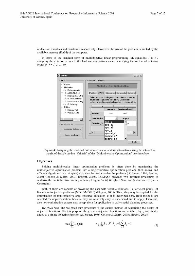
The “Criteria” sub section is used to assign the modeled criterion scores to the land use alternatives by an interactive matrix. Therein, the columns are representing the land use alternatives (e.g. winter wheat, pasture, cf. figure 3), whereas the rows are representing the criteria under consideration (cf. figure 4). The drop down list of the matrix cells provide the user with a list of attributes of the selected criterion layer (cf. sub section “Problem”). Linking a certain criterion score with a land use alternative is done by selecting the appropriate attribute from the appropriate drop down list (i.e. matrix cell). The dimension of the matrix may be adjusted by the arrow buttons on top and on the left hand side of the matrix. Concerning the underlying solver library lp_solve, in principal, there is no fixed limit with respect to the size of the optimization problem (i.e. the number


of decision variables and constraints respectively). However, the size of the problem is limited by the available memory (RAM) of the computer.

In terms of the standard form of multiobjective linear programming (cf. equations 1 to 4), assigning the criterion scores to the land use alternatives means specifying the vectors of criterion scores cj (j = 1, 2, …, n).

Figure 4: Assigning the modeled criterion scores to land use alternatives using the interactive matrix of the sub section “Criteria” of the “Multiobjective Optimization” user interface.

Objectives

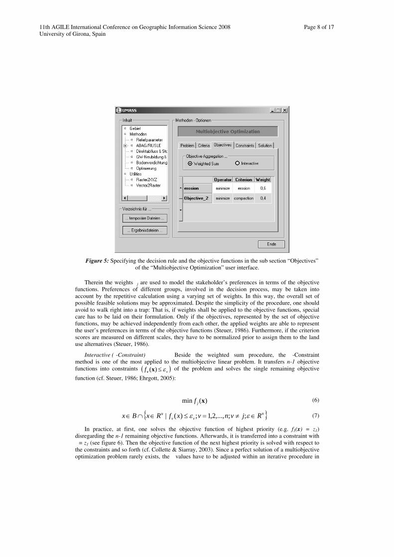
Solving multiobjective linear optimization problems is often done by transferring the multiobjective optimization problem into a singleobjective optimization problem. Well-known and efficient algorithms (e.g. simplex) may then be used to solve the problem (cf. Steuer, 1986; Benker, 2003; Collette & Siarry, 2003; Ehrgott, 2005). LUMASS provides two different procedures to scalarize the multiobjective linear problem (cf. figure 5): (i) Weighted Sum, and (ii) Interactive (i.e. �- Constraint).

Both of them are capable of providing the user with feasible solutions (i.e. efficient points) of linear multiobjective problems (MOLP/MOILP) (Ehrgott, 2005). Thus, they may be applied for the optimization of multiobjective areal resource allocation as it is described here. Both methods are selected for implementation, because they are relatively easy to understand and to apply. Therefore, also non-optimization experts may accept them for application in daily spatial planning processes.

Weighted Sum The weighted sum procedure is the easiest method of scalarizing the vector of objective functions. For this purpose, the given n objective functions are weighted by �j and finally added to a single objective function (cf. Steuer, 1986; Collette & Siarry, 2003; Ehrgott, 2005):

with: (5) jj ∑

=

=>∈∈n

∑=

n

jjj f

1

)(max xλ jnRBx

1

1,0,, λλλ


Figure 5: Specifying the decision rule and the objective functions in the sub section “Objectives” of the “Multiobjective Optimization” user interface.

Therein the weights �j are used to model the stakeholder’s preferences in terms of the objective functions. Preferences of different groups, involved in the decision process, may be taken into account by the repetitive calculation using a varying set of weights. In this way, the overall set of possible feasible solutions may be approximated. Despite the simplicity of the procedure, one should avoid to walk right into a trap: That is, if weights shall be applied to the objective functions, special care has to be laid on their formulation. Only if the objectives, represented by the set of objective functions, may be achieved independently from each other, the applied weights are able to represent the user’s preferences in terms of the objective functions (Steuer, 1986). Furthermore, if the criterion scores are measured on different scales, they have to be normalized prior to assign them to the land use alternatives (Steuer, 1986).

Interactive (�-Constraint) Beside the weighted sum procedure, the �-Constraint method is one of the most applied to the multiobjective linear problem. It transfers n-1 objective functions into constraints ( )vf ε≤)(xv of the problem and solves the single remaining objective

function (cf. Steuer, 1986; Ehrgott, 2005):

)(min xjf (6)

{ }nvv

u RjvnvxfRxBx ∈≠=≤∈∩∈ εε ;;,...,2,1;)(| (7)

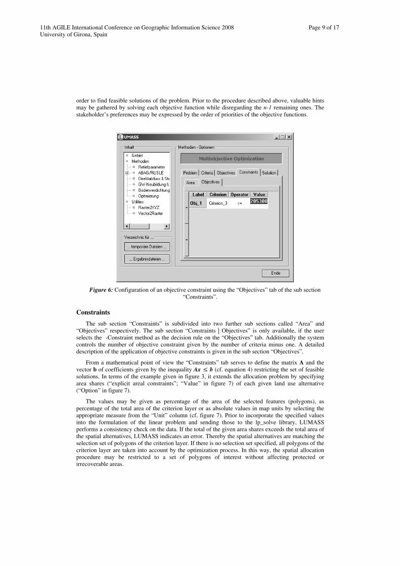
In practice, at first, one solves the objective function of highest priority (e.g. f1(x) = z1) disregarding the n-1 remaining objective functions. Afterwards, it is transferred into a constraint with � = z1 (see figure 6). Then the objective function of the next highest priority is solved with respect to the constraints and so forth (cf. Collette & Siarray, 2003). Since a perfect solution of a multiobjective optimization problem rarely exists, the � values have to be adjusted within an iterative procedure in


order to find feasible solutions of the problem. Prior to the procedure described above, valuable hints may be gathered by solving each objective function while disregarding the n-1 remaining ones. The stakeholder’s preferences may be expressed by the order of priorities of the objective functions.

Figure 6: Configuration of an objective constraint using the “Objectives” tab of the sub section “Constraints”.

Constraints

The sub section “Constraints” is subdivided into two further sub sections called “Area” and “Objectives” respectively. The sub section “Constraints | Objectives” is only available, if the user selects the �-Constraint method as the decision rule on the “Objectives” tab. Additionally the system controls the number of objective constraint given by the number of criteria minus one. A detailed description of the application of objective constraints is given in the sub section “Objectives”.

From a mathematical point of view the “Constraints” tab serves to define the matrix A and the vector b of coefficients given by the inequality Ax ≤ b (cf. equation 4) restricting the set of feasible solutions. In terms of the example given in figure 3, it extends the allocation problem by specifying area shares (“explicit areal constraints”; “Value” in figure 7) of each given land use alternative (“Option” in figure 7).

The values may be given as percentage of the area of the selected features (polygons), as percentage of the total area of the criterion layer or as absolute values in map units by selecting the appropriate measure from the “Unit” column (cf. figure 7). Prior to incorporate the specified values into the formulation of the linear problem and sending those to the lp_solve library, LUMASS performs a consistency check on the data. If the total of the given area shares exceeds the total area of the spatial alternatives, LUMASS indicates an error. Thereby the spatial alternatives are matching the selection set of polygons of the criterion layer. If there is no selection set specified, all polygons of the criterion layer are taken into account by the optimization process. In this way, the spatial allocation procedure may be restricted to a set of polygons of interest without affecting protected or irrecoverable areas.


Figure 7: Configuration of explicit areal constrains (i.e. specifying area shares of the land use alternatives).

According to the domain of the decision variables xi, a user specified area share of the land use alternative Or is given by one of the following expressions (cf. “Explicit Areal Constraint” in figure 3):

∑=

≤m

iw

ri bx

1

continuous / integer (8)

∑=

≤m

iw

rii bxG

1

binary (9)

Therein bw denotes the user specified area shares expressed in map units and Gi denotes the area of the spatial alternative (polygon) Fi. In case of integer decision variables, the given area shares as well as the area of the spatial alternatives are rounded to integer values. In order to ensure that the total quantity of land use alternatives Or allocated to a spatial alternative Fi does not exceed its area, the following constraints (cf. “Implicit Areal Constraint” in figure 3) are additionally managed by LUMASS:

∑=

==p

rwi

ri bGx

1

continuous / integer (10)

∑=

==p

rwi

rii bGxG

1

binary (11)


Solution

The sub section “Solution” provides the user with means to solve, evaluate and map the decision problem at hand. In response of using the “Solve Problem” button, LUMASS reads the user configuration specified in the subsections of the user interface and checks the data in terms of consistency (cf. sub section “Constraints”). Then the given spatial decision problem is mapped into the variables and methods of the lp_solve library. Afterwards, the result of the optimization process is reported within the user interface and may be saved to a text file. Additionally to a brief summary of the decision problem, the report includes the result of the objective functions as well as the results of the inequality constraints (i.e. areal and eventually objective constraints). But most importantly, it also reports the return status of the solver library, which indicates if a feasible solution of the problem exists (cf. figure 8).

Figure 8: The sub section “Solution” of the LUMASS “Multiobjective Optimization” module.

If the user is satisfied with the solution and decides to map it, LUMASS translates the lp_solve result back into a spatial representation (cf. figure 9). Therefore p+1 data fields (OPTr_VAL) are

added to the attribute table of the criterion layer which store the values of the decision variables of

the land use alternatives O

rix

r (cf. figure 10). The additional field OPT_STR serves as value field of the randomly generated unique value legend. It holds the criterion labels (cf. sub section “Criteria”, figure 4) for each criterion whose assigned value of the decision variable is greater than zero.


Figure 9: The automatically generated map as final result of a land use optimization problem.

Figure 10: The representation of optimization results in the attribute table of the criterion layer.


SAMPLE APPLICATION OF THE LUMASS MODULE “MULTIOBJECTIVE OPTIMIZATION”

The application of the LUMASS module “Multiobjective Optimization” is demonstrated using a rather simple but comprehensible optimization problem. The task is to optimize the land use pattern of the investigation site (cf. figure 11) with respect to the minimization of the overall soil erosion. Therefore two scenarios, which differ in the given area shares of the land use alternatives, (cf. table 1) are investigated.

• Scenario 1)

• WW-WB-R

• (c-factor: 0.072)

• Winter Wheat

• (c-factor: 0.115)

• Corn

• (c-factor: 0.505)

• Pasture

• (c-factor: 0.004)

• 1 • ≥ 40

• ≥ 20 • ≥ 6 • ≥ 9

• 2 • ≥ 35

• ≥ 15 • ≥ 6 • ≥ 20

• 1) the values represent the specified area shares as percentage of total

• ww: winter wheat, wb: winter barley, r: rape

Table 1: Scenario definition of the sample application.

Here, the disposition to water driven soil erosion of each land use alternative is expressed in terms of the c-factor. A high value denotes a high disposition to soil erosion and vice versa. Then for each optimization criterion (here: soil erosion), each spatial alternative has to be evaluated with respect to the given land use alternatives. In case of LUMASS, the built in erosion model is used to build the vector of criterion scores as input for the optimization module. Figure 11 maps the results of the model run in terms of a winter wheat – winter barley – rape rotation, which indicates the parcel specific potential erosion risk as well.


Figure 11: Modeled soil erosion for a winter wheat – winter barley – rape rotation.

Solving the optimization problem subject to scenario 1 (cf. table 1 and figure 12, left), it becomes evident, that the optimization procedure assigns the land use alternatives exhibiting a relatively high disposition to soil erosion to those parcels indicated by a relatively low potential erosion risk and vice versa. Adjusting the explicit areal constraints subject to scenario 2, the optimization module produces a similar land use pattern, except that the overall area of parcels providing a relatively high potential erosion risk has become smaller due to the higher percentage of pasture (cf. figure 12, right).


Figure 12: The optimized land use patterns with respect to the minimization of soil erosion and subject to given area shares; left: scenario 1; right: scenario 2

CONCLUSIONS

Using modern software component technologies (e.g. COM, DLL) may facilitate the integration of GIS and additional software packages. This supports the development of powerful and intelligent planning tools that are fully operational in daily planning. The sample application of the module “Multiobjective Optimization” shows plausible land use patterns with respect to the given criteria and subject to the given areal constraints. Due to its generic implementation the application of the optimization module is not restricted to ecological criteria, instead, social or economical criteria may also be taken into account. A drawback of the present system is its limited capabilities considering the geometry and topological structure of the spatial alternatives within the optimization procedure. Concerning the latter, only spatial relationships to parcels that are not under consideration may be specified indirectly.

BIBLIOGRAPHY

Aerts, J. C. J. H., Heuvelink, G. B. M., 2002 Using Simulated Annealing for Resource Allocation. In: International Journal of Geographical Information Science, 16(6), 571-587.

Benker, H., 2003 Mathematische Optimierung mit Computeralgebrasystemen.

Berkelaar, M., Eikland, K., Notebaert, P., 2004 lp_solve Version 5.1 - Open Source (Mixed-Integer) Linear Programming system. http://groups.yahoo.com/group/lp_solve, Date of access: 04.01.2005.

http://groups.yahoo.com/group/lp_solve


Chakhar, S., Martel, J.-M., 2003 Enhancing Geographical Information Systems Capabilities with Multi-Crietria Evaluation Functions. In: Journal of Geographic Information and Decision Analysis, 7(2), 47-71.

Clayton, D., Waters, N., Distributed Knowledge, Distributed Processing, Distributed Users: Integrating Case-based Reasoning and GIS for Multicriteria Decision Making. In: J.-C. Thill (ed.). Spatial Multicriteria Decision Making and Analysis - A Geographic Information Sciences Approach: 275-307, 1999.

Collette, Y., Siarry, P., 2003 Multiobjective Optimization: Principles and Case Studies Decision Engineering.

Denzer, R., Generic Integration in Environmental Information and Decision Support Systems. In: A. E. Rizzoli, A. J. Jakeman (eds.). Integrated Assessment and Decisoin Support, Proceedings of the First Biennial Meeting of the International Environmental Modelling and Software Society iEMSs, 53-60, 2002.

Djokic, D., Toward a General-Purpose Decision Support System Using Existing Technologies. In: M. F. Goodchild, L. T. Steyaert, B. O. Parks, C. Johnston, D. Maidment, M. Crane, S. Glendinning (eds.). GIS and Environmental Modeling: Progress and Research Issues: 353-356, 1996.

Eastman, J. R., 2003 Decision Support: Decision Strategy Anaylsis. In: IDRISI Kilimanjaro - Guide to GIS and Image Processing, 145-166.

Ehrgott, M., 2005 Multicriteria Optimization.

Eldrandaly, K., Eldin, N., Sui, D., 2003 A COM-based Spatial Decision Support System for Industrial Site Selection. In: Journal of Geographic Information and Decision Analysis, 7(2), 72-92.

Fedra, K., Reitsma, R. F., Decision Support And Geographical Information Systems. In: H. J. Scholten, J. C. H. Stillwell (eds.). Geographical Information Systems for Urban and Regional Planning: 177-188, 1990.

Fischer, G., Makowski, M., Land Use Planning. In: A. P. Wierzbicki, M. Makowski, J. Wessels (eds.). Model-Based Decision Support Methodology with Environmental Applications: 333-365, 2000.

Grabaum, R., Meyer, B. C., Mühle, H., 1999 Landschaftsbewertung und -optimierung. Ein integratives Konzept zur Landschaftsentwicklung. UFZ-Bericht, 32.

Jankowski, P., 1995 Integrating Geographical Information Systems and Multiple Criteria Decision-Making Methods. In: International Journal of Geographical Information Science, 9(3), 251-273.

Janssen, R., Rietveld, P., Multicriteria Analysis and Geographical Information Systems: An Application to Agricultural Land Use in the Netherlands. In: H. J. Scholten, J. C. H. Stillwell (eds.). Geographical Information Systems for Urban and Regional Planning: 129-139, 1990.

Löwe, P., 2004 A Spatial Decision Support System for Radarmeteorology Data in South Africa. In: Transactions in GIS, 8(2), 235-244.

Marinoni, O., 2005 A Stochastic Spatial Decision Support System Based on PROMETHEE. In: International Journal of Geographical Information Science, 19(1), 51-68.

Malczewski, J., 1999 GIS and Multicriteria Decision Analysis.

Malczewski, J., 2006 GIS-based multicriteria decision analysis: a survey of the literature. In: International Journal of Geographical Information Science, 20(7), 703-726.


Poch, M., Comas, J., Rodriguez-Roda, I., Sanchez-Marre, M., Cortes, U., 2004 Designing and building real environmental decision support systems. In: Environmental Modelling & Software, 19, 857-873.

Pullar, D., 1999 Using an Allocation Model in Multiple Criteria Evaluation. In: Journal of Geographic Information and Decision Analysis, 3(2), 9-17.

Steuer, R. E., 1986 Multiple criteria optimization: theory, computation, and application. Wiley series in probability and mathematical statistics.

Tkach, R. J., Simonovic, S. P., 1997 A New Approach to Multi-criteria Decision Making in Water Resources. In: Journal of Geographic Information and Decision Analysis, 1(1), 25-44.

Tourino, J., Parapar, J., Doallo, R., Boullon, M., Rivera, F. F., Bruguera, J. D., Gonzales, X. P., Crecente, R., Alvarez, C., 2003 A GIS-Embedded System to Support Land Consolidation Plans in Galicia. In: International Journal of Geographical Information Science, 17(4), 377-396.

Walser, J. P., 1999 Integer Optimization by Local Search - A Domain-Independent Approach.

Wierzbicki, A. P., Makowski, M., Wessels, J. (eds.), 2000 Model-Based Decision Support Methodology with Environmental Applications.

Yialouris, C. P., Kollias, V., Lorentzos, N. A., Kalivas, D., Sideridis, A. B., 1997 An Integrated Expert Geographical Information System for Soil Suitability and Soil Evaluation. In: Journal of Geographic Information and Decision Analysis, 1(2), 89-99.

a gis-based module for the multiobjective optimization of ... · based module for the...

Documents