Proceedings of the 2014 Winter Simulation Conference A. Tolk, S. D. Diallo, I. O. Ryzhov, L. Yilmaz, S. Buckley, and J. A. Miller, eds.

A GLOBAL APPROACH FOR DISCRETE RATE SIMULATION

Cecile Damiron David Krahl

Imagine That Inc.

6830 Via Del Oro, Suite 230 San Jose, CA 95119, USA

ABSTRACT

Before the introduction of discrete rate simulation (DRS), simulating mixed continuous and discrete event (hybrid) systems presented unique challenges that existing simulation methodologies were not suited or adaptable enough to solve. In the 1990’s a new simulation methodology, discrete rate simulation, was developed to address those issues. The most challenging aspect of discrete rate simulation is to accurately calculate the movement of material (“flow”) over a wide range of simulated systems. To calculate flow rates, the first generation DRS technology used an iterative algorithm based on the propagation of potential rates. The iterative approach failed to provide an accurate calculation of flow for many DRS models, limiting the use of this technology to a small range of real world problems. Discussed here is how the second generation DRS technology uses a global oversight approach to model the full range of DRS systems and resolve the issues associated with earlier methods.

1 INTRODUCTION

Discrete rate simulation models the rate-based movement or flow of material between locations, calculating new flow rates when events occur. The materials could be liquids, solids, gases, particles, data, or any other type of fungible or bulk element. Industrial areas where discrete rate simulation is used include bulk material handling, traffic, pipelines, and high speed/large volume production lines.

While the types of problems that discrete rate simulation is designed to solve have always existed, discrete rate simulation is a relatively new development in simulation technology. This combination of the event scheduling features of discrete event simulation with the rate-based capabilities of continuous simulation uniquely addresses a range of systems that cannot be adequately modeled using the discrete event or continuous simulation methods.

Early discrete rate simulation utilized potential rates and iteration algorithms to calculate the flow within these types of systems. A newer global oversight approach utilizes linear programming (LP) to define the problem then solves the LP to maximize rates when algebraic methods are insufficient. The global approach has been proven to be a reliable, computationally efficient, and broadly adaptable DRS technology.

This paper describes discrete rate simulation, compares it to the already well known continuous and discrete event methodologies, and gives an historical perspective. Accurately routing the flow is shown to be the cornerstone of DRS. After showing the usefulness of advanced routing options, the next section presents the iterative approach and its pitfalls. The global oversight approach, implemented in ExtendSim in 2007, is then introduced with its advantages. Finally a real world example of a mine-to-market supply chain simulation illustrates the efficiency and accuracy of the global approach.

Damiron and Krahl

2 DISCRETE RATE SIMULATION

Discrete rate simulation (DRS) is used to model linear continuous systems, hybrid systems, and any other high speed/large volume system that involves the rate-based movement or flow of material from one location to another. During the simulation run, the flow moves at a certain speed, called the effective rate; between events the rate of flow stays constant. The movement of material between locations that hold or route the flow follows paths, rules, and constraints that are set in the model (ExtendSim User Guide 2013). Calculation occurs only at discrete events - such as equipment failure, a product change-over, or a tank reaching full capacity - that would cause a change to one or more effective rates.

There is no concept of delta time (Δt) in discrete rate simulation. Instead, the simulation clock updates only when events occur. The discrete event calendar used by the discrete rate simulation maintains a list of future planned events. It is interesting to note that a single event may be rescheduled many times, adapting its predicted time of occurrence because of other system events. For example, if the flow rate into a tank changes, the predicted time that a tank will be full or empty is adjusted.

2.1 Compared to Continuous and Discrete Event Simulation

Discrete rate simulation is similar to continuous simulation in that they both simulate flow and recalculate flow rates, which are continuous variables. DRS differs from continuous simulation in that it is event-based; it does not simulate every time step. DRS is also similar to discrete event simulation in that both utilize event-based timing. However, while discrete event simulation assumes there is no change in the system between consecutive events, in a DRS model flow continues to move between events, although at a constant rate. Furthermore, DRS models are concerned with the status (quantity and location) of homogeneous flow, rather than the status of discrete system entities.

The issues when trying to model a discrete rate system using continuous or discrete event simulation has been well documented (Sturrock and Drake 1996, Damiron and Nastasi, 2008, Nutaro et al. 2012). If a linear continuous system is modeled with continuous simulation, a time step must be chosen that is sufficiently small to minimize error. Since state change events can occur between time steps, precision errors will happen no matter how small the time step is. Plus smaller time steps negatively affect model performance. If the system is modeled as discrete event, the modeler must choose a “chunk size” or amount of material that a single item represents, dividing the flow into discrete entities. When flow is artificially discretized, the simulation has the same precision issues as with continuous. Here, as well, the modeler will have to trade off accuracy for performance. Neither continuous nor discrete event simulation are as accurate for linear continuous systems as discrete rate, and the approximations and assumption caused by those two approaches often resulted in models that were poor predictors of the real-world systems (Sturrock and Drake 1996).

Figure 1 illustrates the difference in behavior between the three modeling methods in a now classic simulation model of a tank that alternately fills and empties. (Damiron and Nastasi 2008, Krahl 2009, Béchard and Côté 2013) The continuous and discrete event models both show increasing error as the simulation progresses.

Figure 1: Discrete rate, continuous, and discrete event simulation compared

Damiron and Krahl

2.2 Background

Simulation modeling for industries that operate rate-based and hybrid systems has the same objectives as modeling for any other industrial area – how best to design and configure the processes, analyze capacity, maximize throughput, and plan for the future. However, as discussed above, modelers have historically encountered obstacles when trying to simulate hybrid systems using existing methodologies (Sturrock and Drake 1996). This was due to the inherent differences when modeling high speed and large volume processes, the homogeneous properties of the materials being modeled, and the continuous or discrete event formalism of the existing commercial tools (Nutaro 2012). As a consequence, the technology for modeling hybrid systems evolved significantly over the past 20 years.

The first generation DRS tool was developed in the early 1990’s when it was recognized that a new simulation methodology was needed (Siprelle and Parsons 1995). Termed “discrete rate simulation” (Siprelle et al. 1999), this new architecture utilized the discrete event clock but moved flow through the system at rates that maintained mass balance. In this first generation, the routing of the flow was resolved through iteration. If a calculation resulted in a change to one of the input rates, the calculation was iterated until a steady state rate, or a steady state rate within a given tolerance (Béchard and Côté 2013), was detected.

Experience with the iterative approach showed that it had some serious pitfalls when used to model actual systems. Specifically, as the model became more complex with flows merging and diverging and as real-world rules needed to be incorporated into the model, calculations would become unstable or simply wrong. It became apparent that a new method was required if discrete rate simulation were to make the jump from a consulting tool to one suitable for commercial off the shelf (COTS) applications.

In the mid 2000’s a new approach was developed that is computationally efficient, ensures accurate interactions between discrete event and continuous elements, and is adaptable to a wide range of applications. This second generation technology has a global oversight approach that utilizes linear programming (LP) to define and solve the problem when modeling discrete rate systems.

3 MASS BALANCE, MAXIMIZATION, AND ROUTING

In order to fully grasp the benefit of the global approach, it is helpful to understand that routing - merging and diverging of flow - is a critical aspect of DRS systems. And the importance of rules that specify how flow is routed becomes very clear when discussing mass balance and flow maximization.

Definition 1 Effective rate: The actual rate of movement, expressed as a quantity of flow per time unit. Definition 2 Supply rate: The incoming rate as if there were no downstream capacity limitation. Definition 3 Demand rate: The outgoing rate as if there were infinite material availability upstream.

3.1 Mass Balance and Maximization

A basic tenet of discrete rate simulation is to maximize the flow while maintaining mass balance. When merging and diverging flow, these two principles alone are not enough to specify a unique way of directing the flow for each stream.

Consider the example of a component that receives flow at a supply rate of 9 tons per hour and divides the flow into three streams, each with a demand rate of 7 tons per hour. The maximization principle ensures that 9 tons per hour will flow through the component and the mass balance principle ensures that the sum of the 3 exiting streams will equal 9. However, there are an infinite number of ways the flow could be divided between the 3 streams while still respecting mass balance. For example, the top stream could receive 1 ton per hour and the other two streams receive 4 tons each. Or the upper stream could receive nothing, the middle steam could receive 7 tons per hour, and the lower stream could receive 2 tons per hour. Since the supply rate is 9 and the sum of the 3 demand rates is 21, 12 (21-9) represents

Damiron and Krahl

the excess demand over the supply; it also represents the area of possible choices for how the flow could be distributed.

3.2 Routing Rules

The types of systems modeled using DRS have multiple flow streams that merge and diverge. A modeler needs to be able to control and predict how flow will be routed within the model. For this reason, each component routing the flow has to have a set of rules to choose from that will provide a unique “predictable” way to describe how flow should travel through the system.

How each stream sends and receives flow is governed by routing rules that can be generally divided into fixed and non-fixed rules. Using a fixed rule means that, no matter what happens in the rest of the model, the rule's formula will be strictly followed. In contrast, a non-fixed rule is flexible. Its rule is followed only if model conditions allow it; otherwise, maximizing flow takes precedence and the rule expresses a preference rather than a strict formula for how the flow is merged or diverged.

Fixed and non-fixed rules both respect the maximization and mass balance principles. In addition, each rule ensures that there is a unique optimal solution for how to divide the flow between streams. One specificity of a fixed rule is that the rule itself can limit the overall flow going through the system. The non-fixed rule on the other end ensures that as much flow as possible will go through.

The distinction between fixed and non-fixed routing rules is important. Experience has shown that non-fixed rules are essential when modeling discrete rate systems. And, as will be shown in the following section, the iterative approach can fail when using a non-fixed rule.

3.3 Comparing a Fixed and Non-Fixed Rule

There are a range of routing rules. This discussion is limited to two comparable rules: the proportional, a fixed rule, and the distributional, a non-fixed rule. Table 1 compares these two rules. In the table:

• all variables are positive (≥ 0) • x is the effective inflow rate, y is the effective outflow rate • n is the number of streams • pi represents the proportions between streams with 𝑝! = 1, 𝑝! ≥ 0!

!!! • S are slack variables • i, j represent indexes from 0 to n

Table 1: Proportional and Distributional Rules

Rule Type Diverge Component Mathematical Equation

Proportional Fixed

Constraints: 𝑦! = 𝑝! ∗ 𝑥 𝑖 = 0 𝑡𝑜 𝑛

Distributional Non-fixed

𝑚𝑎𝑥: 𝑛𝑥 + −!

!!! 𝑆!" (𝑤𝑖𝑡ℎ 𝑖 ≠ 𝑗)!!!!

Constraints: −𝑥 + 𝑦! = 0!

!!! 𝑝! ∗ 𝑦! − 𝑝! ∗ 𝑦! + 𝑆!" − 𝑆!" = 0

With i and j combination without repetition !!!!

The proportional and distributional rules both route flow based on a percentage for each output. In the

proportional mode the percentages at each outflow path must be observed regardless of the system state. This is a straightforward calculation. However, in the diverging distributional mode these proportions serve as rules for the branches only when the proportional demands exceed supply. When demand

%

pp

p

x01

n

yy

y

01

n

dpp

p

x01

n

yy

y

01

n

Damiron and Krahl

exceeds supply for a component, the proportions assigned to each branch are used as preferences to determine how the limited supply should be distributed across the outflow branches. However, when the supply is greater than or equal to the demand, the diverging component passes as much flow through each branch as the demand will allow and the proportions are ignored.

3.4 Why Non-Fixed Rules are Necessary

Consider a simple process of material in one tank being transferred to three tanks. Outflow of the source tank is limited to 9 units of flow per time unit. Inputs to the three downstream tanks are limited to 1.6, 9, and 9 units of flow per time unit respectively. The diverge rule is to send equal proportions to each tank.

Table 2 highlights the difference in behavior for the fixed and non-fixed rules. For the fixed proportional rule shown on the left, the solution is obvious as each output branch would be limited to receiving 1.6 units of flow per time unit. However, for the non-fixed distributional rule there is a range of optimal solutions. The question then becomes what is the correct way to balance flow between the streams using the proportions of the non-fixed rule when there is excess demand in the system. The optimal solution, shown on the right, routes as much as possible to the top tank (1.6 units) while splitting the remaining supply of 7.4 units equally between the two remaining tanks. This solution not only maintains mass balance and maximizes the flow but also balances flow as equally as possible.

Table 2: Diverging Flows

Proportional Fixed Rule Distributional Non-Fixed Rule

Mathematical representation:

𝑦! = 13 𝑥

𝑦! = 13 𝑥

𝑦! = 13 𝑥

Mathematical representation: 𝑚𝑎𝑥: 3𝑥 − 𝑆!" − 𝑆!" − 𝑆!" − 𝑆!" − 𝑆!" − 𝑆!"

Constraints: −𝑥 + 𝑦! + 𝑦! + 𝑦! = 0 𝑦! − 𝑦! + 𝑆!" − 𝑆!" = 0 𝑦! − 𝑦! + 𝑆!" − 𝑆!" = 0 𝑦! − 𝑦! + 𝑆!" − 𝑆!" = 0

Mathematical representation from the valve components: 𝑥 ≤ 9; 𝑦! ≤ 1.6; 𝑦! ≤ 9; 𝑦! ≤ 9 As seen in the example, the fixed proportion rule is restrictive and limits the overall amount of

product moving through the system. Mass balance is maintained, but this is the only solution possible in order to maximize the flow while respecting the fixed proportions defined by the component. On the other hand, the non-fixed distributional rule allows the modeler to maximize the flow as much as the mass balance only rule would but also allows the modeler to specify “preferences” on how to divide the flow when there is an area of optimal solutions. In a non-fixed rule the proportion between streams is not known in advance and strongly depends on the state of the system surrounding the routing component.

For example: the proportional fixed rule represents a recipe with a fixed mix of ingredients; the distributional non-fixed rule represents liquid circulating along pipes where the proportions are guidelines based on the physical properties of the system. Most DRS models require a mix of all the rules to

1.6

4.8/9%

1.6/9

1.6/9Fixed rule

1/31/31/3

1.6

9d

3.7/9

3.7/9Non-fixed rule

1/31/31/3

Damiron and Krahl

accurately represent a real world system. However, as shown in the next two sections, the iterative approach can fail when non-fixed rules are used. The global approach has none of those issues.

4 ITERATIVE APPROACH

In the iterative approach paradigm, the effective rate is the minimum between the supply and demand rates. Information about potential rates is obtained by propagating the rates through all the connected components of a model.

The supply rate is propagated in the same direction as the flow. Each component receives information from its inflow connection reporting how much flow it would receive if there were no downstream limitation. The component is then in charge of propagating downstream what its upstream potential rate is, given its own status and the upstream potential rate it received.

The demand rate is propagated in the opposite direction of the flow. Each component receives information from its outflow connection reporting how much flow it can receive if there were an infinite upstream supply. The component is then in charge of propagating upstream what its downstream potential rate is, given its own status and the downstream potential rate it received.

For a model built as a straight line, the iterative approach is perfectly valid. Limits to this approach arise when diverging and merging flow gets more involved, especially if non-fixed rules are used or the system has feedback loops.

4.1 Issues When Calculating the Effective Rate

Figure 2 shows how supply and demand is calculated in the iterative approach when there is a diverge component set to a non-fixed distributional rule:

Figure 2: Diverging Flows, Iteration approach

To calculate the supply rates, a hypothetical model is created in sequence for each stream as if an empty tank were placed directly after that stream. The potential rate for the stream is then the effective rate at that location. This case reveals two issues with the use of the potential rate concept.

Iteration assumes the supply and demand are independent but they are not. The supply rate for each stream does not exclusively depend on the supply rate it receives but depends also on the demand rate of the other streams. This makes the propagation of the information much more complicated because in order for the diverge component to provide the supply rate, it needs information from the demand rate. The two propagations of demand rate and supply rate are thus interdependent and, depending on which loop is the starting point, iteration can provide different answers.

Iteration does not always respect mass balance. If the supply rate is summed, it is obvious that the mass balance is not respected:

𝑥! < 𝑦!!!!!! 𝑖𝑚𝑝𝑙𝑖𝑒𝑠 9 < 3.25 + 3.7 + 4.9 𝑖𝑚𝑝𝑙𝑖𝑒𝑠 9 < 11.85.

When the supply rate is defined on a per stream basis and the total amount of flow is examined, the diverge receives a supply rate of 9 but it can potentially distribute 11.85. When the model gets complex, this can cause accuracy and stability issues.

Demand propagates right to left Supply propagates left to right d

9

1/31/31/3

3.25

3.7

4.9

1.6

2.5

9

13.1

Damiron and Krahl

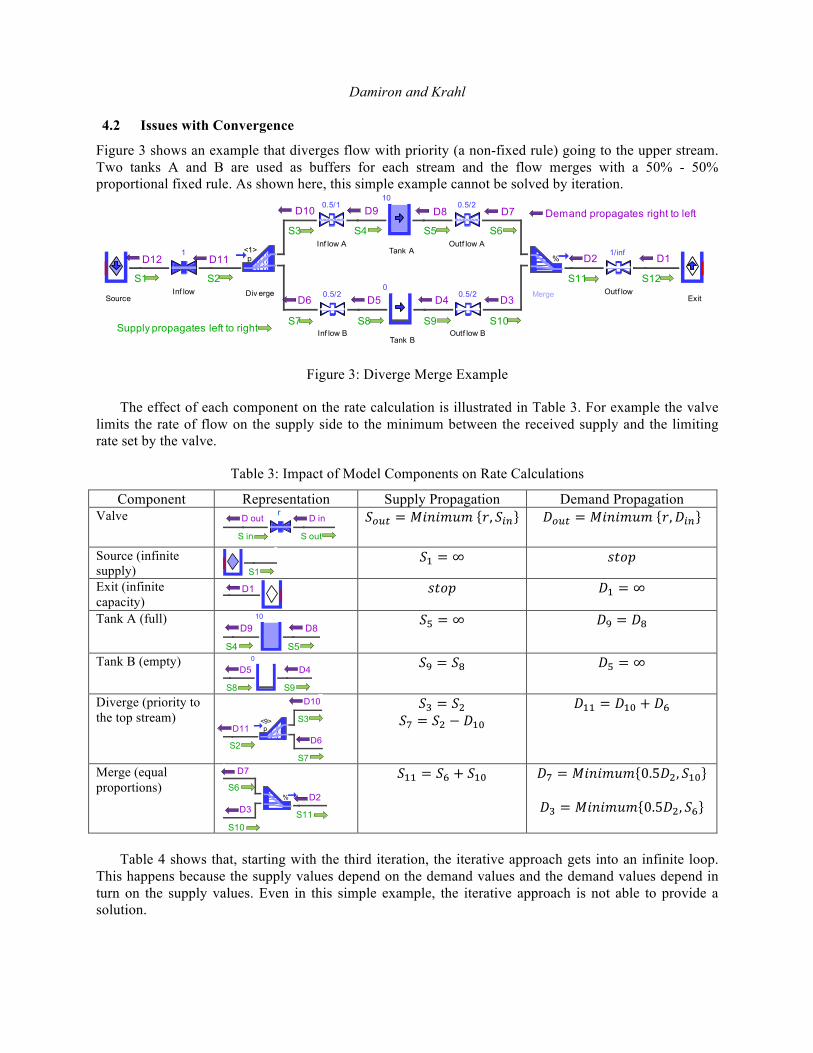
4.2 Issues with Convergence

Figure 3 shows an example that diverges flow with priority (a non-fixed rule) going to the upper stream. Two tanks A and B are used as buffers for each stream and the flow merges with a 50% - 50% proportional fixed rule. As shown here, this simple example cannot be solved by iteration.

Figure 3: Diverge Merge Example

The effect of each component on the rate calculation is illustrated in Table 3. For example the valve limits the rate of flow on the supply side to the minimum between the received supply and the limiting rate set by the valve.

Table 3: Impact of Model Components on Rate Calculations

Component Representation Supply Propagation Demand Propagation Valve

𝑆!"# = 𝑀𝑖𝑛𝑖𝑚𝑢𝑚 𝑟, 𝑆!" 𝐷!"# = 𝑀𝑖𝑛𝑖𝑚𝑢𝑚 𝑟,𝐷!"

Source (infinite supply)

𝑆! = ∞ 𝑠𝑡𝑜𝑝

Exit (infinite capacity)

𝑠𝑡𝑜𝑝 𝐷! = ∞

Tank A (full)

𝑆! = ∞ 𝐷! = 𝐷!

Tank B (empty)

𝑆! = 𝑆! 𝐷! = ∞

Diverge (priority to the top stream)

𝑆! = 𝑆! 𝑆! = 𝑆! − 𝐷!"

𝐷!! = 𝐷!" + 𝐷!

Merge (equal proportions)

𝑆!! = 𝑆! + 𝑆!" 𝐷! = 𝑀𝑖𝑛𝑖𝑚𝑢𝑚 0.5𝐷!, 𝑆!"

𝐷! = 𝑀𝑖𝑛𝑖𝑚𝑢𝑚 0.5𝐷!, 𝑆!

Table 4 shows that, starting with the third iteration, the iterative approach gets into an infinite loop.

This happens because the supply values depend on the demand values and the demand values depend in turn on the supply values. Even in this simple example, the iterative approach is not able to provide a solution.

Source

1

Inf low

p<1>

Div erge

0.5/1

Inf low A

10

Tank A

0.5/2

Outf low A

%

Merge Exit0.5/2

Inf low B

0

Tank B

0.5/2

Outf low B

1/inf

Outf low

Supply propagates left to right

Demand propagates right to left

D1D2

D3D4D5D6

D7 D8D9D10

D11D12

S1 S2

S3 S4 S5 S6

S7 S8 S9 S10

S11 S12

Source

1p

<8>

Div erge

D inD out

S in S out

r

1

S11/inf

D1

0.5/1

Inf low A

100.5/2

Outf low A

D8D9

S4 S5

0.5/2

Inf low B

00.5/2

Outf low B

D4D5

S8 S9

1

Inf low

p<9>

0.5/1

0.5/2D6

D10

D11

S2

S3

S70.5/2

%0.5/2

1/inf

Outf low

D2D3

D7

S6

S10S11

Damiron and Krahl

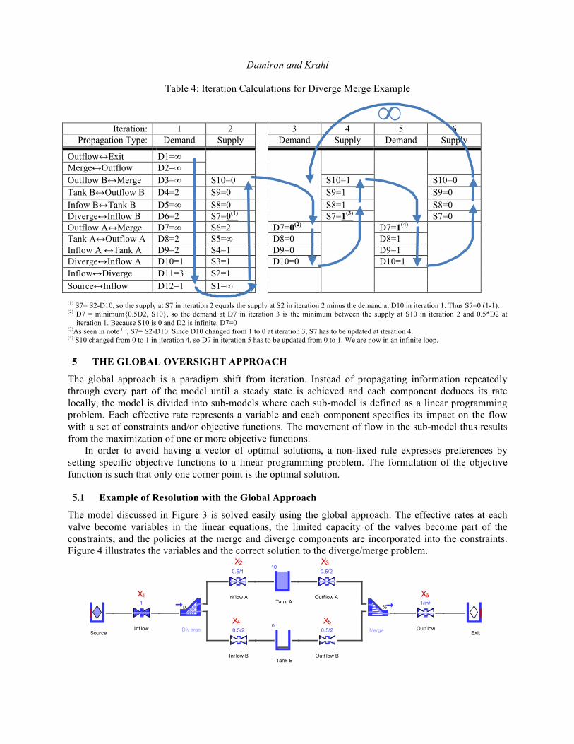
Table 4: Iteration Calculations for Diverge Merge Example

Iteration: 1 2 3 4 5 6 Propagation Type: Demand Supply Demand Supply Demand Supply

Outflow↔Exit D1=∞ Merge↔Outflow D2=∞ Outflow B↔Merge D3=∞ S10=0 S10=1 S10=0 Tank B↔Outflow B D4=2 S9=0 S9=1 S9=0 Infow B↔Tank B D5=∞ S8=0 S8=1 S8=0 Diverge↔Inflow B D6=2 S7=0(1) S7=1(3) S7=0 Outflow A↔Merge D7=∞ S6=2 D7=0(2) D7=1(4) Tank A↔Outflow A D8=2 S5=∞ D8=0 D8=1 Inflow A ↔Tank A D9=2 S4=1 D9=0 D9=1 Diverge↔Inflow A D10=1 S3=1 D10=0 D10=1 Inflow↔Diverge D11=3 S2=1 Source↔Inflow D12=1 S1=∞

(1) S7= S2-D10, so the supply at S7 in iteration 2 equals the supply at S2 in iteration 2 minus the demand at D10 in iteration 1. Thus S7=0 (1-1). (2) D7 = minimum{0.5D2, S10}, so the demand at D7 in iteration 3 is the minimum between the supply at S10 in iteration 2 and 0.5*D2 at

iteration 1. Because S10 is 0 and D2 is infinite, D7=0 (3)As seen in note (1), S7= S2-D10. Since D10 changed from 1 to 0 at iteration 3, S7 has to be updated at iteration 4. (4) S10 changed from 0 to 1 in iteration 4, so D7 in iteration 5 has to be updated from 0 to 1. We are now in an infinite loop.

5 THE GLOBAL OVERSIGHT APPROACH

The global approach is a paradigm shift from iteration. Instead of propagating information repeatedly through every part of the model until a steady state is achieved and each component deduces its rate locally, the model is divided into sub-models where each sub-model is defined as a linear programming problem. Each effective rate represents a variable and each component specifies its impact on the flow with a set of constraints and/or objective functions. The movement of flow in the sub-model thus results from the maximization of one or more objective functions.

In order to avoid having a vector of optimal solutions, a non-fixed rule expresses preferences by setting specific objective functions to a linear programming problem. The formulation of the objective function is such that only one corner point is the optimal solution.

5.1 Example of Resolution with the Global Approach

The model discussed in Figure 3 is solved easily using the global approach. The effective rates at each valve become variables in the linear equations, the limited capacity of the valves become part of the constraints, and the policies at the merge and diverge components are incorporated into the constraints. Figure 4 illustrates the variables and the correct solution to the diverge/merge problem.

Source

1

Inf low

p

Div erge

0.5/1

Inf low A

10

Tank A

0.5/2

Outf low A

%

Merge Exit0.5/2

Inf low B

0

Tank B

0.5/2

Outf low B

1/inf

Outf low

X1

X2 X3

X4 X5

X6

∞

Damiron and Krahl

Figure 4: Variables for Diverge Merge Example

The variables, constraints, and objective function for the problem are shown in Table 5. The LP problem is first pre-solved algebraically to reduce the number of variables and constraints. The resulting linear equations are solved with a linear programming solver. In this example a problem which seems to be 6 variables and 5 constraints ends up being a 4 variables, 3 constraints problem.

Table 5: Diverge Merge Problem Solved with Global Approach

Problem Set by the Model Components Problem to Optimize After Pre-Solve Treatment Global variables:X1, X2, X3, X4, X5, X6 Global variables: X1, X2, X3, X6

Maximization: 2𝑋! + 𝑋!(from Diverge) Maximization: 2𝑋! + 𝑋! Constraints:

C1: −𝑋! + 𝑋! + 𝑋! = 0 (from Diverge) C2: 𝑋! − 𝑋! ≤ 0 (from Tank A) C3: −𝑋! + 𝑋! ≤ 0 (from Tank B) C4: −𝑋! + 0.5𝑋! = 0 (from Merge) C5: −𝑋! + 0.5𝑋! = 0 (from Merge)

Constraints: C1: −𝑋! + 𝑋! + 𝑋! = 0 C2: 𝑋! − 0.5𝑋! ≤ 0 C3: −𝑋! + 0.5𝑋! ≤ 0

Upper bounds: B1: X1<=1 (from Inflow) B2: X2<=1 (from Inflow A) B3: X3<=2 (from Outflow A) B4: X4<=2 (from Inflow B) B5: X5<=2 (from Outflow B)

Upper bounds: B1: X1<=1 B2: X2<=1 B3: X4<=2 B4: X6<=4

5.2 Advantages of the Global Approach

The global approach has a number of advantages over iterative methods. For instance, when there is some degree of flexibility in the system, it balances the flow between branches without the modeler having to define limits based on each possible model state. It is also more reliable than the iterative approach, especially when the system involves routing or feedback loops. Overall, models simulated with the global approach are more reflective of real world conditions.

In addition, the fact that any DRS sub-model can be represented as a linear programming problem takes advantage of the large amount of work done over the years on operations research. Calculating the effective rates in a model becomes a generic and straight forward linear programming problem.

Listed below are some properties making a DRS linear programming problem simple to solve: • A basic feasible solution always exists in a DRS LP problem. In fact, having no flow circulating

in a DRS sub-model (all variables equal 0) is always a solution even if it is not “the” optimal solution. It is an advantage to have a basic feasible solution because it proves that the LP is always “feasible” and given a basic feasible solution the simplex algorithm efficiently moves to a better adjacent basic feasible solution (Chinneck 2008).

• Unbounded solutions are discarded since each flow has a maximum rate. Associated with the existence of at least one feasible solution, this property insures that the problem has at least one optimal solution.

• There are no integer variables or special ordered sets, which makes the problem faster to solve. It might seem at first blush that the computational complexity of the LP solution is dependent on

problem size. This incorrectly assumes that each time effective rates have to be calculated, the entire model is solved using an LP. However, using an LP is, in fact, an efficient approach:

• Only the portions of the model that need it are reevaluated at each event. • If an algebraic solution suffices, it will be used instead of the LP to solve for the effective rates.

Damiron and Krahl

• Each time an area generates an LP problem, a simplification is done to decrease the size of the

LP. For example each constraint of form 𝑥! = 𝑝! ∗ 𝑦 can, after transformation, reduce the LP problem by one less variable and at least one less constraint.

• Upper bounds constraints should not be counted in the number of overall constraints when the computational complexity is evaluated. The reason is that the LP program uses the Upper Bound technique (Hillier and Lieberman, 1995).

Unlike the iterative approach, the complexity of the algorithm does not increase with the complexity of the model. With the global approach, when each type of component has defined how it impacts the flow, the number of instances of the same component does not add to the complexity of the algorithm.

6 A COAL SUPPLY CHAIN EXAMPLE

A mine-to-market model is being used in the ongoing analysis of a coal supply chain. The model has been designed to test stockpile management strategies in a planned materials handling facility (MHF) and to test competing capital investment options for moving coal from the MHF to a planned rail head. An overview of this model is shown in Figure 5.

The primary input to the model is a time-based mine plan containing the specific seam, raw coal amounts, wash plant yield, and the concentrations of chemical constituents for each parcel of coal. After delivery by a haul truck fleet into hoppers feeding the wash plants, the washed coal is conveyed and stacked according to the defined strategy. Reclaiming is triggered by trains and is handled in such a way as to try to blend coal from the available MHF stockpiles as close to final product target specification as possible. In this way, as many trains leaving the MHF as possible will contain product coal on specification, reducing or eliminating the need for downstream blending at the bulk handling port. The model is stochastic and requires multiple trials to generate decision quality results.

This model utilizes a variety of fixed and non-fixed rules for merging flow, truck-level movement of ore at the mine, numerous transitions from flow to discrete entity and back, flow properties indicating the constituents of the ore, and sophisticated logic representing the blending process of the ore. It represents the processing of approximately 700,000 tons of ore each month.

Figure 5: Mine to Market Coal Supply Chain Model

The mine-to-market system is represented in the model by 750 components, 252 DRS components, and 59 DRS routing components. It includes 158 effective rates. Simulating 1 month of operations results in: • Total simulation events: 868,498, total effective rate calculations: 60,997, total optimization solves:

91,289.

Waste Out

Waste Out

Damiron and Krahl

• Per optimization call, the average number of variables is 8.3 with a maximum of 18 and the average

number of constraints is 6.6 with a maximum of 13.

7 CONCLUSION

There are a variety of reasons why a global approach should be used to calculate the maximum flow of material through a simulation model. These generally become evident to the model builder using an older iteration-based technology. Merging and diverging capabilities need to be completely modular, a feedback loop cannot be an issue, no matter how complex the system to model is, the model needs to provide a robust solution.

The global oversight approach is a complete shift of paradigm. A DRS system is now seen as a linear programming problem to optimize. Each effective rate is a variable, each component specifies its impact on the flow with a set of constraints and eventually objective functions to maximize, and the set of effective rates is deduced from one or multiple maximizations of objective functions.

This modern system for resolving rates in discrete rate simulations has proven to be a robust, scalable technology. Solving a single equation in one step yields a more reliable and accurate solution. The global approach has been used in a variety of models and industries since its introduction in 2007 (Sharda and Bury 2008, Savrasovs 2012).

REFERENCES

Béchard, V., and N. Côté. 2013. “Simulation of Mixed Discrete and Continuous Systems: an Iron Ore Terminal Example.” In Proceedings of the 2013 Winter Simulation Conference, edited by R. Pasupathy, S.-H. Kim, A. Tolk, R. Hill, and M. E. Kuhl, 1167-1178. Piscataway, New Jersey: Institute of Electrical and Electronics Engineers, Inc.

Chinneck, J. 2008. Feasibility and Infeasibility in Optimization Algorithms and Computational Methods. New York, New York: Springer Science + Business Media, LLC.

Damiron, C. and A. Nastasi. 2008. “Discrete Rate Simulation Using Linear Programming.” In Proceedings of the 2008 Winter Simulation Conference, edited by S. J. Mason, R. R. Hill, L. Moench, O. Rose, 740-749. Piscataway, New Jersey: Institute of Electrical and Electronics Engineers, Inc.

Hillier, F. S. and G. J. Lieberman. 1995. Introduction to Operations Research, 6th ed. Stanford, California: McGraw Hill.

Imagine That Inc. 2013. ExtendSim User Guide, San Jose, California. Krahl, D. 2009. “ExtendSim Advanced Technology: Discrete Rate Simulation.” In Proceedings of the

2009 Winter Simulation Conference, edited by M. D. Rossetti, R. R. Hill, B. Johansson, A. Dunkin, and R. G. Ingalls, 333–338. Piscataway, New Jersey: Institute of Electrical and Electronics Engineers, Inc.

Nutaro, J., P.T. Kuruganti, V. Protopopescu, and M. Shankar. 2012. “The Split System Approach to Managing Time in Simulations of Hybrid Systems having Continuous and Discrete Event Compo-nents”. SIMULATION 88 (3):281-298.

Savrasovs, M. 2012 “Traffic Flow Simulation on Discrete Rate Approach Base.” In Transport and Telecommunication, 2012, 13 (2), 167-173.

Sharda, B., and S. J. Bury. 2008. “A Discrete Event Simulation Model for Reliability Modeling of a Chemical Plant.” In Proceedings of the 2008 Winter Simulation Conference, edited by S. J. Mason, R. R. Hill, L. Monch, O. Rose, T. Jefferson, J. W. Fowler, 1736-1740. Piscataway, New Jersey: Institute of Electrical and Electronics Engineers, Inc.

Siprelle, A. J. and D. J. Parsons. 1995. “Modeling a Bulk Manufacturing System Using Extend.” In Proceedings of the 1995 Winter Simulation Conference, edited by C. Alexopoulos, K. Kang, W. R. Lilegdon, and D. Goldsman, 813-817. Piscataway, New Jersey: Institute of Electrical and Electronics Engineers, Inc.

Damiron and Krahl

Siprelle, A. J., D. J. Parsons, and R. A. Phelps. 1999. “SDI Industry Pro: Simulation for Enterprise-Wide

Problem Solving.” In Proceedings of the 1999 Winter Simulation Conference, edited by P. A. Farrington, H. B. Nembhard, D. T. Sturrock, and G. W. Evans, 241-248. Piscataway, New Jersey: Institute of Electrical and Electronics Engineers, Inc.

Sturrock, D. T. and G. R. Drake. 1996. “Simulation for High-Speed Processing”. In Proceedings of the 1996 Winter Simulation Conference , edited by J. M. Charnes, D. J. Morrice, D. T. Brunner, and J. J. Swain, 432-436. Piscataway, New Jersey: Institute of Electrical and Electronics Engineers, Inc.

AUTHOR BIOGRAPHIES

CECILE DAMIRON is a Simulation Software Engineer at Imagine That Inc. She received her Masters of Science in Econometrics and completed postgraduate specialized studies in the use of computer science/engineering in economic analysis & decision-making at the University Lumiere Lyon II at Lyon (France). Before joining Imagine That Inc. in 2004, Ms. Damiron worked for 7 years as a simulation consultant at 1Point2 in France. She can be contacted by email at ceciled@extendsim.com DAVID KRAHL is the Technology Evangelist with Imagine That Inc. He received an MS in Project and Systems Management in 1996 from Golden Gate University and a BS in Industrial Engineering from the Rochester Institute of Technology in 1986. Mr. Krahl has worked extensively with a range of simulation programs including ExtendSim, SLAM II, TESS, Factor, AIM, GPSS, SIMAN, XCELL+ and MAP/1. A few of the companies that Mr. Krahl has worked with as a consultant and educator are Chrysler, U.S. National Park Service, Idaho National Engineering Laboratory, United Technologies, and Boeing. He is actively involved in the simulation community. Mr. Krahl is a Certified Analytics Professional. His email address is davek@extendsim.com.