A Global Geometric Framework for Nonlinear Dimensionality Reduction

Joshua B. Tenenbaum (Stanford), Vin de Silva (Stanford), John C. Langford (CMU)

SCIENCE 2000

Presented by: Mingyuan Zhou

Duke University, ECE

April 3, 2009

Outline

• Motivations

• PCA, Principle Component Analysis

• MDS, Multidimensional Scaling

• Isomap, Isometric Feature Mapping

• Examples

• Summary

Motivations

• Finding meaningful low-dimensional structures hidden in their high-dimensional observations

High-dimensional sensory input, Human Brain, a small number of perceptually relevant features

High-dimensional data, Machine Learning, relevant low dimensional features

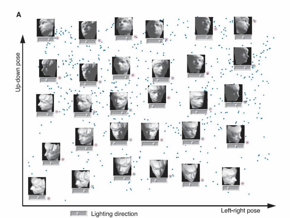
• Discovering the nonlinear degrees of freedom underling complex natural observations: human handwriting, face images, Swiss roll ….

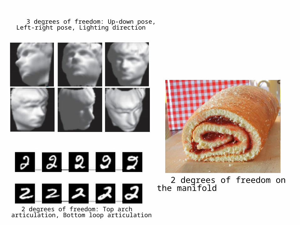
3 degrees of freedom: Up-down pose, Left-right pose, Lighting direction

2 degrees of freedom: Top arch articulation, Bottom loop articulation

2 degrees of freedom on the manifold

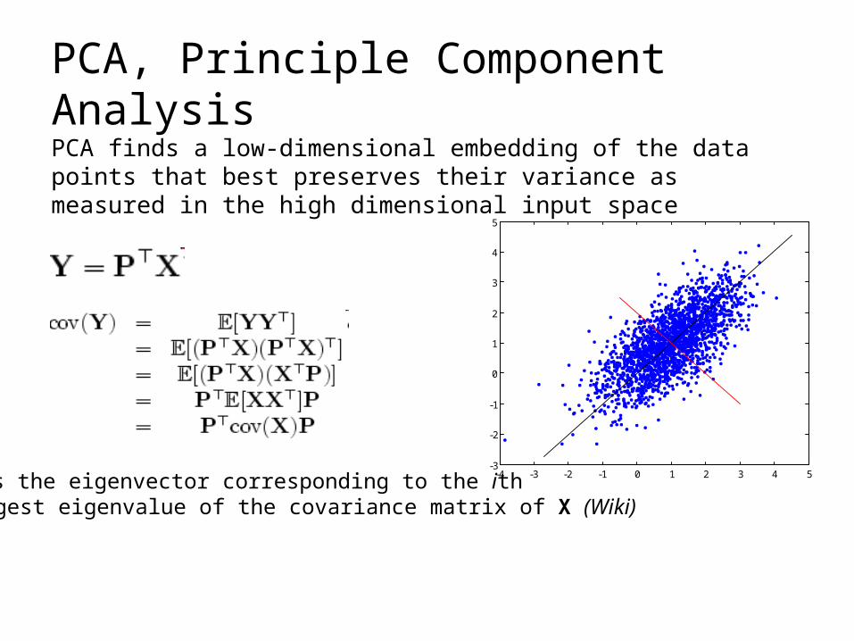
PCA, Principle Component AnalysisPCA finds a low-dimensional embedding of the data points that best preserves their variance as measured in the high dimensional input space

Pi is the eigenvector corresponding to the ithlargest eigenvalue of the covariance matrix of X (Wiki)

-4 -3 -2 -1 0 1 2 3 4 5-3

-2

-1

0

1

2

3

4

5

MDS, Multidimensional Scaling

ij

2( )stress

scaleij ijd

MDS finds an embedding that preserves the pairwise distances (or generalized disparities) between data points, equivalent to PCA when those distances are Euclidean. “An MDS algorithm starts with a matrix of item–item similarities, then assigns a location to each item in N-dimensional space, where N is specified a priori. For sufficiently small N, the resulting locations may be displayed in a graph or 3D visulization.” Wiki

ijdObjective: choose to minimize the stress, where is the Euclidian distance between points i and j on the map, and is the dissimilarity between them.

ijd

Advantages and Limitations of PCA and MDS

Advantages• Computational efficiency• Global optimality• Asymptotic convergence guarantees

Limitations• Many data sets contain essential nonlinear structures that are invisible to PCA and MDS. (The failure of the Euclidean structure in the input space)

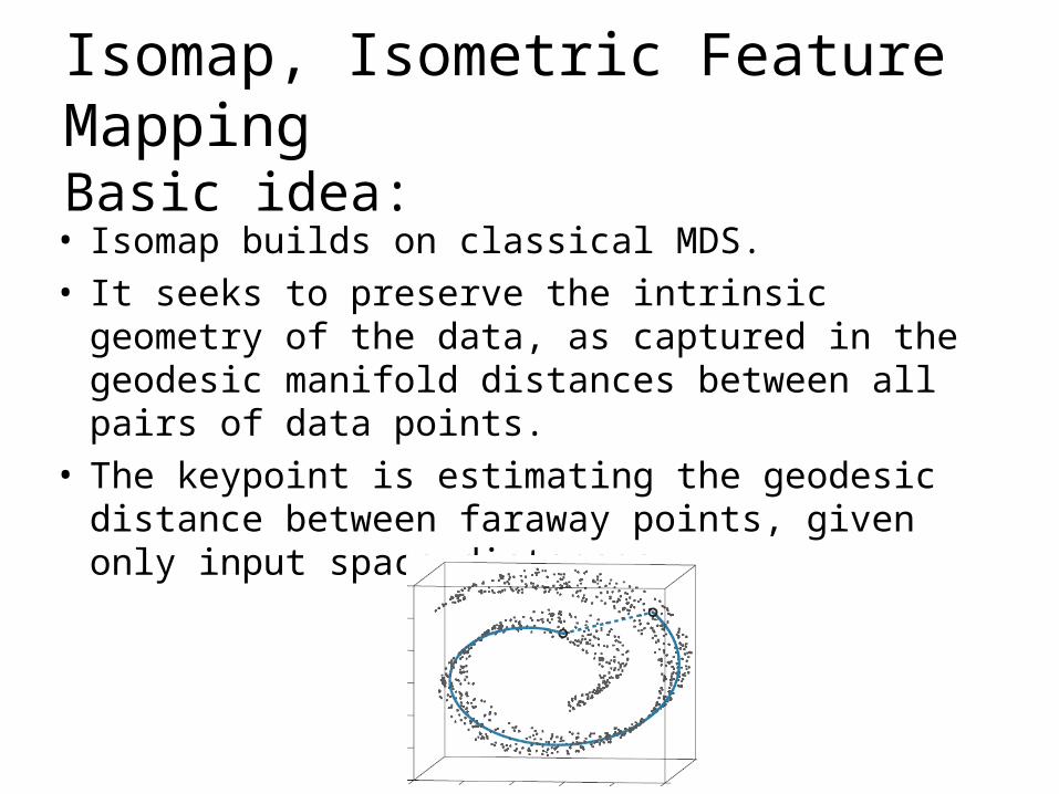
Isomap, Isometric Feature MappingBasic idea:

• Isomap builds on classical MDS.• It seeks to preserve the intrinsic geometry of the

data, as captured in the geodesic manifold distances between all pairs of data points.

• The keypoint is estimating the geodesic distance between faraway points, given only input space distances.

Isomap: Algorithms• Step 1: Based on the distance in the input space

(fixed radius or K nearest neighbors), determining which points are neighbors on the Manifold M.

These neighborhood relations are represented as a weighted graph G over the data points.

( , )Xd i j

Isomap: Algorithms• Step 2: Estimating the geodesic distances between

all pairs of points on the manifold M by computing their shortest path distances in the graph G.

A simple algorithm:

( , )Md i j

( , )Gd i j

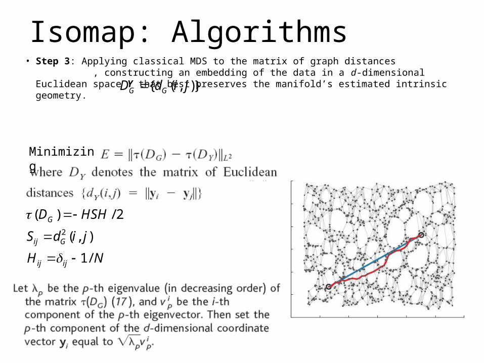
Isomap: Algorithms• Step 3: Applying classical MDS to the matrix of graph distances ,

constructing an embedding of the data in a d-dimensional Euclidean space Y that best preserves the manifold’s estimated intrinsic geometry.

{ ( , )}G GD d i j

2

( ) / 2

( , )

1/

G

ij G

ij ij

D HSH

S d i j

H N

Minimizing

Isomap: Examples

Performance comparison

A. Face images varying in pose and illumination

B. Swiss roll data

PCA, MDS

Isomap

PCA, MDS

Isomap

Summary

• Isomap is capable of discovering the nonlinear degrees of freedom that underline complex natural observations.

• It efficiently (noniterative, polynomial time) computes a globally optimal solution.

• It is guaranteed to converge asymptotically to the true structure for intrinsically Euclidean manifolds.