a guide to spatial diagnosis of catchment water quality
TRANSCRIPT

A guide to spatial diagnosis of catchment water quality
Technical Report No. 20
September 2010

2 Landscape Logic Technical Report No. 20
Published by Landscape Logic, Hobart Tasmania, September 2010.This publication is available for download as a PDF from www.landscapelogicproducts.org.au
Cover photo: View towards Duck Bay. Photographer: Kirsten Verburg
Contact: Dr Kirsten Verburg, CSIRO Land and Water, GPO Box 1666, Canberra ACT [email protected]
Preferred citation: Verburg K, Creswell H and Bende-Michl U (2010) A guide to spatial diagnosis of catchment water quality, Landscape Logic Technical Report no. 20, Hobart.
CSIRO advises that the information contained in this publication comprises general statements based on scientific research. The reader is advised and needs to be aware that such information may be incomplete or unable to be used in any specific situation. No reliance or actions must therefore be made on that information without seeking prior expert professional, scientific and technical advice. To the extent permitted by law, CSIRO (including its employees and consultants) excludes all liability to any person for any consequences, including but not limited to all losses, damages, costs, expenses and any other compensation, arising directly or indirectly from using this publication (in part or in whole) and any information or material contained in it.
ISBN 978-0-9807946-9-4
LANDSCAPE LOGIC is a research hub under the Commonwealth Environmental Research Facilities scheme, managed by the Department of Environment, Water Heritage and the Arts. It is a partnership between: • six regional organisations – the North Central, North East
& Goulburn–Broken Catchment Management Authorities in Victoria and the North, South and Cradle Coast Natural Resource Management organisations in Tasmania;
• five research institutions – University of Tasmania, Australian National University, RMIT University, Charles Sturt University and CSIRO; and
• state land management agencies in Tasmania and Victoria – the Tasmanian Department of Primary Industries & Water, Forestry Tasmania and the Victorian Department of Sustainability & Environment.
The purpose of Landscape Logic is to work in partnership with regional natural resource managers to develop decision-making approaches that improve the effectiveness of environmental management.Landscape Logic aims to:1. Develop better ways to organise existing knowledge and
assumptions about links between land and water management and environmental outcomes.
2. Improve our understanding of the links between land management and environmental outcomes through historical studies of private and public investment into water quality and native vegetation condition.
NORTH CENTRALCatchment
ManagementAuthority
3A guide to spatial diagnosis of catchment water quality
A guide to spatial diagnosis of catchment water qualityKirsten Verburg, Hamish Cresswell, Ulrike Bende-Michl CSIRO Water for a Healthy Country National Research Flagship
SummaryTargeting actions to address water quality issues within catchments requires an understanding of how the catchment ‘works’. It is important to know which nutrients, and in what form, contribute to the prob-lem, the origin of the nutrients, and the location of critical source areas within the catchment. Knowledge of the nutrient pathways and when they reach the stream is also critical – not only for the choice of man-agement action, but also for the design of monitoring to evaluate its effectiveness. In other words, for management actions to be efficient and useful they need to be underpinned by a spatial ‘diagnosis’ of catchment water quality.
A range of different types of information can contribute to such a diagnosis and often complement each other. To form a diagnosis, one effectively combines different ‘lines of evidence’. In many research studies, this process is applied informally. The approach put forward in this guide aims to make it a more transparent process, based on a framework for organising available evidence and integrating that knowledge into a spatial diagnosis. This multiple lines of evidence framework can also assist catchment managers with the cost-effective choice of methods.
The Guide explains the multiple lines of evidence diagnosis framework and describes the individual methods using a step-by-step approach, along with their input and analysis requirements. Some of these methods rely on readily available existing information and their description focuses on how to get the most out of the data. Other methods relate to new data collection for which monitoring design principles are given. The strengths and weaknesses of different methods are identified, as well as powerful com-binations. To illustrate the application of the various methods and the synthesis of the information into a spatial diagnosis the Guide also includes a worked example from the Duck River catchment in NW Tasmania, Australia.

4 Landscape Logic Technical Report No. 20
Acknowledgments
AuthorsKirsten Verburg, Hamish Cresswell and Ulrike Bende-Michl, CSIRO Water for a Healthy Country Flagship, CSIRO Land and Water
Comments and feedbackPeter Hairsine, CSIRO Land and WaterJohn Gibson, TAFITed Lefroy, University of TasmaniaKevin Petrone, CSIRO Land and WaterAniela Grun, NRM SouthPat Feehan, Goulburn-Broken CMADebbie Searle and Andrew Baldwin, NRM NorthSue Botting, Cradle Coast NRMGreg Pinkard, University of TasmaniaKate Hoyle and Kate Wilson, DPIPWE
FundingDepartment of Environment, Water Heritage and the Arts (CERF Landscape Logic program)CSIRO Water for a Healthy Country FlagshipCSIRO Land and Water
Case study fieldwork and assistance, catchment visitsSeija Tuomi, Chris Drury, Danny Hunt, Gordon McLachlan, Tim Ellis, CSIRO Land and WaterValerie Latham, Susan Reynolds, CSIRO Marine and Atmospheric ResearchLachlan Newham, Australian National UniversityJohn Gibson, Steven McGowan, TAFI/University of TasmaniaRegina Magierowski, David Oldmeadow, UTASMr and Mrs Wells, Mr and Mrs Ollington, Land ownersDonald Rockcliffe and Ian Houshold, DPIPWEKaylene Allen, NRM South
Advice, assistance or input to analysis methods and data provisionJames Foley, John Gallant, Trevor Dowling, Andrew Herczeg, CSIRO Land and WaterGrant Dickins, Gang-Jun Liu, RMITBill Cotching, Shane Broad, TIARJohn Gibson, TAFIBrent Henderson, CSIRO Mathematics, Informatics and StatisticsAndrew Herczeg, Fred Leaney, CSIRO Land and WaterCarol Kendall, Steven Silva, Megan Young, U.S. Geological Survey, Menlo Park CABrett McGlone and Darryl Johnson , Incitec Pivot LimitedAndrew Moy, Antarctic and Climate and Ecosystems CRCKate Hoyle, Kate Wilson, David Krushka, DPIPWESue Botting, Cradle Coast NRMFarmers and locals in Duck River catchment
Project communication supportLiam Gash, University of TasmaniaGreg Pinkard, University of TasmaniaMark Smith, DairyTasRosie James, TIARCircular Head Council

5A guide to spatial diagnosis of catchment water quality
Contents
1. Introduction 6
2. Making a catchment diagnosis 72.1 Overview of methods 82.2 Putting it together – the spatial catchment diagnosis 10
3. Methods 113.1 Initial spatial conceptual modelling 113.2 Spatial source area likelihood estimation (SSALE) 153.3 Spatial ‘snapshot’ surveys 193.4 Event monitoring 223.5 High frequency monitoring 243.6 Isotope and tracer analyses 27
4. Duck River catchment case study 294.1 Description 294.2 Initial spatial conceptual modelling 314.3 Spatial Source Area Likelihood Estimation 344.4 Spatial ‘snapshot’ surveys 384.5 High frequency monitoring 434.6 Isotope and tracer analyses 454.7 Putting it together – the spatial catchment diagnosis 49
Appendix A: Spatial source area likelihood estimation (SSALE) 56

6 Landscape Logic Technical Report No. 20
Catchment water quality management interventions are usually prompted by condition assessments (e.g. ANZECC 2000 guidelines) or ecological indicators (e.g. the Queensland Ecosystem Health Monitoring Program report cards), or a specific observed impairment of the river or the receiving water body. The management objectives set in relation to these interventions typically are responses to biophysical, social and economic drivers. From a biophysical point of view, to be cost effective and efficient these interventions need to be implemented in the most appropriate locations. Where high levels of sedi-ment or nutrients are of concern there is, therefore, a need to understand ‘how a catchment works’ with respect to their delivery into rivers and streams. This means answering key questions, including:1. Which forms of nitrogen, phosphorus or sedi-
ments contribute to water quality problems?2. What is their origin?3. Where in the catchment are their source areas?4. Along which hydrological pathways are the
materials transported to the waterways?5. And when?
Effectively this constitutes the development of a spatial catchment ‘diagnosis’, which, similar to a medical diagnosis, is used to inform manage-ment as well as to determine the best strategies for
monitoring the impact of management interventions (Figure 1.1). Different types of complementary information (‘multiple lines of evidence’) are used to develop the diagnosis. In many research stud-ies, this process is applied informally. The approach put forward in this guide aims to make this a more transparent process, based on a framework for organising available evidence and integrating that knowledge into a spatial diagnosis.
The diagnosis framework reflects a multiple lines of evidence approach and highlights the par-ticular strengths of different methods in addressing the 5 questions listed above. Chapter 2 describes this diagnosis framework in more detail. The indi-vidual methods are described using a step-by-step approach in Chapter 3, along with their input and analysis requirements. Some of these methods rely on readily available existing information and the description focuses on how to get the most out of the data. Other methods relate to new data collec-tion for which monitoring design principles are given. The strengths and weaknesses of different methods are also discussed, as well as powerful combinations. Finally Chapter 4 provides a worked example from the Duck River catchment in NW Tasmania, Australia.
1. Introduction
Figure 1.1: Choice and prioritisation of management interventions in response to condition monitoring outcomes requires a spatial ‘diagnosis’ of catchment water quality conditions. This catchment diagnosis uses a range of monitoring data and also informs the type of monitoring suitable for assessments of intervention impact.

7A guide to spatial diagnosis of catchment water quality
Approaches to identifying sources and pathways of nitrogen, phosphorus and sediment within catch-ments have different strengths in relation to the five key questions listed in Section 1. In addition, some methods are useful for forming hypotheses, while others are more suited for testing hypotheses set by other methods. It is recommended that multiple lines of evidence are used for the diagnosis as this provides considerably more confidence for the con-clusions drawn. Table 2.1 shows a framework for applying multiple lines of evidence to address the five key questions from Section 1:1. Which forms of nitrogen, phosphorus or sedi-
ments contribute to water quality problems? Are these nutrients dissolved or attached, organic or inorganic, or are suspended sediments the cause of problems?
2. What is their origin? Are they a consequence of soil erosion, natural mineralisation processes, fer-tiliser inputs, effluent, or a point source?
2. Making a catchment diagnosis
3. Where in the catchment are their source areas? Are these areas linked to intensive land uses? Are they particular locations within the catchment, e.g. steep slopes, certain soil types or areas adjacent to streams?
4. Along which hydrological pathways are the materials transported to the waterways? As sur-face runoff, through the soil as subsurface lateral flow, or groundwater flow?
5. And when? Only during events, or (also) during baseflow periods? Throughout the year, or only in particular seasons?The framework highlights the relative strengths
of a range of methods. It allows selection of the most appropriate methods for different questions. A brief overview of the methods and their strengths is pre-sented next. Underlined methods are discussed in detail in Chapter 3.
Table 2.1: Methods and their areas of strength
Section/Method Constituent/form Origin Source
areas Pathways Timing
3.1 Initial spatial conceptual modelling * * * * *
3.2 Spatial source area likelihood estimation (SSALE)
*** *
3.3 Spatial ‘snapshot’ surveys */*** a) * *** * b)
3.4 Event monitoring */*** a) */*** c) ***
3.5 High frequency monitoring */*** a) * */*** c) ***
3.6 Isotope and tracer analyses *** d) * */*** d)
3.7 Modelling * e) * e) * e) * e) * e)
* Some information, or allowing hypotheses to be formed*** Detailed information, area of strengtha) *** when samples are analysed for constituent formsb) When snapshot surveys are carried out in different seasons, seasonal differences can be established.c) In small catchments (<0.2 km2) the method has been proven useful to identify pathways (e.g. Heathwaite
et al. 1989, Holz 2010), but in larger catchments like the Duck River catchment (542 km2) or even larger ones, high frequency monitoring results are likely to only support hypotheses about possible pathways.
d) Some isotope and tracer analyses have strengths in identifying the origins of nutrients or sediments, others have strengths in identifying water sources or constituent pathways. See Section 3.6.
e) Many different models are available and their strengths will vary according to the type of model, pro-cesses captured, data availability, and mode of use (e.g. predictive or explorative). A discussion of this will be included in a future version of the Guide.
8 Landscape Logic Technical Report No. 20
2.1 Overview of methodsThe condition monitoring, indicators or causal analysis of impairment that prompted the need for a spatial diagnosis of catchment nutrient and sediment sources often already provide some information about the constituent(s) that may be the issue and possibly the timing during the year. A first step in the spatial diagnosis is to interpret these data within the context of a spatial conceptual model of the catchment.
Initial spatial conceptual modelling draws on available information about soils and their distri-bution, land use and its distribution, landform and local climate. It interprets these data to provide a simple synthesis, which is spatial in nature, of the likely hydrology of the catchment and possible source areas and transport processes. This can be presented primarily as a narrative to elucidate feedback from those with knowledge of the catch-ment and to use as a first step in diagnosing how the catchment works in terms of stream, river and estuary water quality. The method provides a docu-mented starting hypothesis, based on best current knowledge, that can point to where more informa-tion is required and what other methods might be valuable for the spatial catchment diagnosis. Some of the strengths of this method include that it can be done fairly quickly, that it can help facilitate integra-tion and data synthesis, and that it can be expressed in a language familiar to local land managers to draw from valuable local knowledge.
If the data on soil type, land use, and terrain are available in a Geographical Information System (GIS), it is often useful to use the spatial source area likelihood estimation (SSALE) method. to explore the spatial location of sources further and obtain more quantitative evidence. It provides a spatial prioritisation of areas within the catchment that are most likely to contribute, and bases this on the con-cept that a critical source area is an area that has both a source and the potential for mobilisation and transport of this source to a receiving body. Source and transport likelihood are explored using a series of decision trees based on soil, land use, rainfall and terrain characteristics that are known to influence source availability and different transport processes. The decision trees and the decision thresholds contained in them are fully transparent and can be adjusted to reflect conditions specific to particular catchments (e.g. informed by the initial conceptual modelling). They can also be used in a non-techni-cal context for NRM/CMA group discussions.
To verify areas identified as potential critical source areas by the initial conceptual modelling and/or the spatial source area likelihood estimation
it is useful to carry out spatial ‘snapshot’ surveys, also referred to as longitudinal or synoptic sampling. It can provide information about the spatial location of point and non-point sources within the catchment, provided these are not short-lived (e.g. spikes in concentrations). During a period of stable flow the river system is sampled at as many points as possi-ble providing a longitudinal profile of water quality, which can be compared with the identified potential critical source areas. The spatial ‘snapshot’ surveys often also identify other unexpected increases or decreases in concentrations along the streams and tributaries that are linked to sources or processes overlooked by the initial conceptual modelling or spatial source area likelihood estimation. This may then prompt some further investigation. Finally, the survey results are useful for improving the spatial conceptual model of the catchment as well. The chemical composition of a stream at any point often reflects the combined impact of several factors such as geology, climatic conditions and land use in its contributing catchment area. Survey results can indicate groups of sites that are affected by similar processes. When the spatial ‘snapshot’ surveys are carried out at different times of the year they can provide some information about seasonal effects and how spatial sources may change in response.
The timing of the spatial ‘snapshot’ surveys dur-ing stable base flow means that they are not suitable for estimation of relative contributions to annual load exports from the catchment, as these occur mainly during storm events. To capture event loads requires sampling with a higher temporal frequency, i.e. event monitoring with auto-samplers, or high frequency monitoring with equipment that allows continuous observation of in-stream nutrient/sedi-ment concentrations (e.g. at 15 min to hourly time scale). These water quality monitoring methods would be used in the spatial catchment diagnosis where there is a need for assessments of loads or information about the conditions under which nutri-ents and sediment are exported from the catchment. This may relate to accurate timing or specification of event types and controlling factors. The analyses typically require information on discharge at the same time scale. The combination of concentra-tion and discharge data can, however, also provide insights into processes that govern catchment scale water quality responses. It can, for example, help form hypotheses on the type of sources and the pathways by which the nutrients may have reached the stream. High frequency monitoring that is not limited to events has in a number of studies proven useful to identify possible point sources and also to help elucidate diurnal processing in-stream. The rel-ative value of event monitoring and high frequency

9A guide to spatial diagnosis of catchment water quality
monitoring depends on the questions one is trying to answer. It is, therefore, important to consider their role within the spatial catchment diagnosis. High fre-quency monitoring usually provides more scope for process interpretations, although this depends on the scale of application. The instruments are also still quite costly. Event monitoring using auto-samplers is often cheaper, but there is a limit to the number of samples that can be taken and the samples need to be collected and analysed in a laboratory. Both methods tend to be applied at catchment or sub-catchment outlets, although event auto-samplers and some high frequency monitoring instruments could be used temporary at key locations in the catchment and then provide a spatial assessment of sources during storm events (to complement simi-lar information from the spatial snapshot surveys for base flow conditions).
When questions of origin or pathway are important, isotope and tracer analyses have often provided powerful evidence. These methods typi-cally require a working hypothesis that can be tested using targeted measurements. They would, therefore, usually be applied after any available water quality data are interpreted in the context of a conceptual model of the catchment. These methods
draw their strength from conservative or predict-able behaviour of constituents in the water and isotopes of the water or the constituents. Some com-monly used methods include natural geochemical tracers, such as alkalinity, Si, Ca, Na, Cl, and TOC, and stable isotope tracers of water (18O, 2H) and of solutes (NO3, PO4, SO4 – 15N, 18O, 34S) and sediments or particulate material (e.g. 15N, 13C, 34S, 87Sr). Radon (222Rn) an odourless and colourless radioactive noble gas that occurs naturally in air, in water, and in rocks and soil is often used pinpoint the location of groundwater –surface water interactions. Many of these require more specialised laboratory analyses and the interpretation of data is often very much a forensic puzzle. Nevertheless their targeted use can improve catchment understanding considerably.
Modelling can potentially contribute towards all 5 questions – depending on the type of model and how the model is used. It is important to realise though that modelling is only one line of evidence and it is typically not where one would start. Building a conceptual model of catchment functioning using a variety of easily available or easily obtainable monitoring data should be a pre-cursor to mod-elling. It can then be applied when and where the diagnosis requires it.

10 Landscape Logic Technical Report No. 20
2.2 Putting it together – the spatial catchment diagnosisIt is difficult to be prescriptive about how a spa-tial catchment diagnosis is put together. Often the knowledge that is obtained by the application of the different methods and the careful consider-ation where this information sits within the multiple lines of evidence framework (Table 2.1) builds up a picture of what is happening in the catchment. To formalise this mental diagnosis it can be useful to document the various pieces of evidence within the multiple lines of evidence diagnosis framework, as shown in Table 4.3 for findings from the Duck River catchment case study. It can also be useful to present findings in a flow diagram to show how the ‘story’ has evolved (see example in Figure 4.26).
One question that is often raised is what to do with contradictory lines of evidence. In other fields where multiple lines of evidence assessments are used some people have taken a (semi-) quantitative approach with relative weights assigned to the dif-ferent lines of evidence on the basis of for example, study design, number of reference or control sites, or study quality (Norris et al. 2005). Most studies, however, use informal applications with ‘best pro-fessional judgement’ (Burton et al. 2002, Chapman et al. 2002) providing the synthesis. We believe that the spatial diagnosis of catchment water quality as presented here also lends itself best to an informal application, especially as it covers multiple aspects (the 5 key questions) and spatially distributed pro-cesses. Most often we are not trying to prove or disprove one hypothesis, but are building up a con-sistent picture or conceptual model.
Nevertheless it can sometimes be useful to reflect on the accumulated evidence, pose some hypotheses and test these. One possible approach to this is shown in Table 2.2, which is adapted from a method used by the Causal analysis and diagnosis decision information system (CADDIS1) developed
by the US EPA to identify stressors that cause bio-logical impairments in aquatic ecosystems (US EPA, 2000). Available evidence can refute or diagnose outright, or support or weaken a case to various degrees. Scores are then evaluated in terms of con-sistency between lines of evidence. Where lines of evidences appear to contradict, this can relate to uncertainties inherent in the method, sampling procedures or interpretation, but it is also quite pos-sible that the conceptual model is not complete. This should, therefore, be an incentive to revisit the conceptual model, rather than straight rejection of the evidence.
ReferencesBurton GA, Chapmen PM, Smith EP (2002) Weight-of-evidence
approaches for assessing ecosystem impairment. Human and Ecological Risk Assessment, 8(7) 1657-1673.
Chapman PM, McDonald BG, Lawrence GS (2002) Weight-of-evidence issues and frameworks for sediment quality (and other) assessments. Human and Ecological Risk Assessment, 8(7), 1489-1515.
Heathwaite AL, Burt TP, Trudgill ST (1989) Runoff, sediment, and solute delivery in agricultural drainage basins: A scale-depen-dant approach, p. 175-190, In: Regional Characterization of Water Quality, IAHS publication no 182.
Holz GK (2010) Sources and processes of contaminant loss from an intensively grazed catchment inferred from patterns in discharge and concentration of thirteen analytes using high intensity sampling. J. Hydrol. 383, 194-208.
Norris R, Liston P, Mugodo J, Nichols S, Quinn G, Cottingham P, Metzeling L, Perriss S, Robinson D, Tiller D, Wilson G (2005) Multiple lines and levels of evidence for detect-ing ecological responses to management intervention. pp. 456-463. In Proceedings of the 4th Australian stream manage-ment conference: linking rivers to landscapes. (Rutherford ID, Wisznieuwski I, Askey-Doran MJ, and Glazik R, Eds.) Department of Primary Industries, Water and Environment, Hobart, Tasmania.
Suter GW, Norton SB, Cormier SM (2002) A methodology for inferring the causes of observed impairments in aquatic eco-systems. Environ Toxicol Chem 21, 1101-1111.
U.S. Environmental Protection Agency (2000) Stressor identifica-tion guidance document. EPA-822-B-00-025. Washington, DC.
Table 2.2: Evidence ‘scoring’ to assess consistency between lines of evidence (adapted from CADDIS, a US EPA system for causal analysis and diagnosis).
Question Hypothesis 1 Hypothesis 2Evidence from method 1 + +
Evidence from method 2 +++ – –
Evidence from method 3 – –
Evidence from method 4 ++ –
Consistency of evidence Supports Weakens
Possible scoring: R refutes, D diagnoses, +++ convincingly supports, --- convincingly weakens, ++strongly supports, – –strongly weakens, + somewhat supports, – somewhat weakens, 0 neither supports nor weakens, NE no evidence
1. The CADDIS system can be accessed at: www.epa.gov/caddis
11A guide to spatial diagnosis of catchment water quality
3. Methods
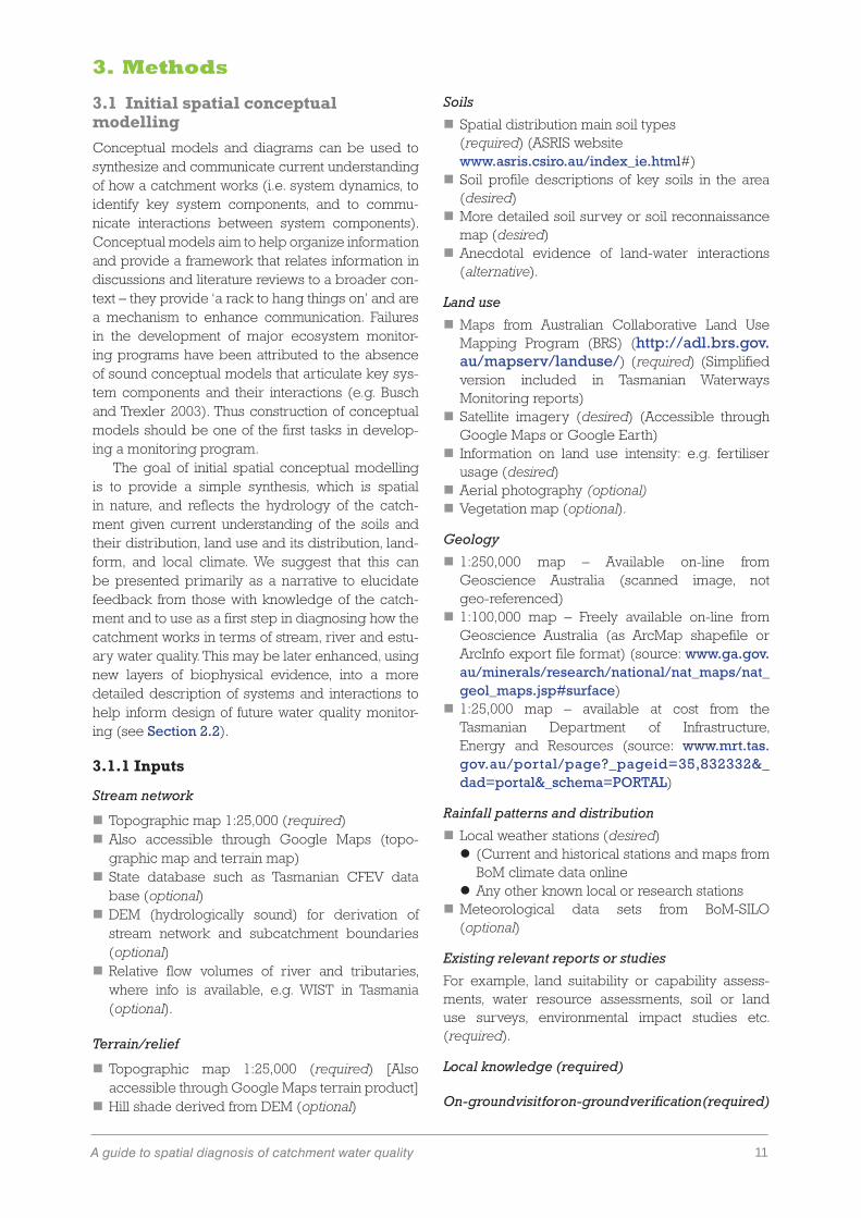
3.1 Initial spatial conceptual modellingConceptual models and diagrams can be used to synthesize and communicate current understanding of how a catchment works (i.e. system dynamics, to identify key system components, and to commu-nicate interactions between system components). Conceptual models aim to help organize information and provide a framework that relates information in discussions and literature reviews to a broader con-text – they provide ‘a rack to hang things on’ and are a mechanism to enhance communication. Failures in the development of major ecosystem monitor-ing programs have been attributed to the absence of sound conceptual models that articulate key sys-tem components and their interactions (e.g. Busch and Trexler 2003). Thus construction of conceptual models should be one of the first tasks in develop-ing a monitoring program.
The goal of initial spatial conceptual modelling is to provide a simple synthesis, which is spatial in nature, and reflects the hydrology of the catch-ment given current understanding of the soils and their distribution, land use and its distribution, land-form, and local climate. We suggest that this can be presented primarily as a narrative to elucidate feedback from those with knowledge of the catch-ment and to use as a first step in diagnosing how the catchment works in terms of stream, river and estu-ary water quality. This may be later enhanced, using new layers of biophysical evidence, into a more detailed description of systems and interactions to help inform design of future water quality monitor-ing (see Section 2.2).
3.1.1 Inputs
Stream network
� Topographic map 1:25,000 (required) � Also accessible through Google Maps (topo-graphic map and terrain map)
� State database such as Tasmanian CFEV data base (optional)
� DEM (hydrologically sound) for derivation of stream network and subcatchment boundaries (optional)
� Relative flow volumes of river and tributaries, where info is available, e.g. WIST in Tasmania (optional).
Terrain/relief
� Topographic map 1:25,000 (required) [Also accessible through Google Maps terrain product]
� Hill shade derived from DEM (optional)
Soils
� Spatial distribution main soil types (required) (ASRIS website www.asris.csiro.au/index_ie.html#)
� Soil profile descriptions of key soils in the area (desired)
� More detailed soil survey or soil reconnaissance map (desired)
� Anecdotal evidence of land-water interactions (alternative).
Land use
� Maps from Australian Collaborative Land Use Mapping Program (BRS) (http://adl.brs.gov.au/mapserv/landuse/) (required) (Simplified version included in Tasmanian Waterways Monitoring reports)
� Satellite imagery (desired) (Accessible through Google Maps or Google Earth)
� Information on land use intensity: e.g. fertiliser usage (desired)
� Aerial photography (optional) � Vegetation map (optional).
Geology
� 1:250,000 map – Available on-line from Geoscience Australia (scanned image, not geo-referenced)
� 1:100,000 map – Freely available on-line from Geoscience Australia (as ArcMap shapefile or ArcInfo export file format) (source: www.ga.gov.au/minerals/research/national/nat_maps/nat_geol_maps.jsp#surface)
� 1:25,000 map – available at cost from the Tasmanian Department of Infrastructure, Energy and Resources (source: www.mrt.tas.gov.au/portal/page?_pageid=35,832332&_dad=portal&_schema=PORTAL)
Rainfall patterns and distribution
� Local weather stations (desired) z (Current and historical stations and maps from BoM climate data online
z Any other known local or research stations � Meteorological data sets from BoM-SILO (optional)
Existing relevant reports or studies
For example, land suitability or capability assess-ments, water resource assessments, soil or land use surveys, environmental impact studies etc. (required).
Local knowledge (required)
On-ground visit for on-ground verification (required)

12 Landscape Logic Technical Report No. 20
3.1.2 Tools
Assessment of typical hydrological behaviour of soils using HOST
HOST (Hydrology of soil types) is a UK soils classifi-cation based on a number of conceptual models that describe dominant hydrological pathways through soil (Boorman et al. 1995). The primary consider-ation within each of the models is at what depth, and for what reason, does lateral water movement become a significant hydrological component.
The models include scenarios such as (a) surface runoff or subsurface lateral flows being dominant due to poor vertical drainage in a soil profile, or (b) where water movement is mainly vertical. Various other models between these two extremes are represented, often with more complexity. Because antecedent water content is a factor controlling soil hydrological response to rainfall, watertable posi-tion is included explicitly. The models represent various physical settings. With available knowledge on the distribution and characteristics of local soils the HOST hydrological classification can be used to group or differentiate soils based on their hydrolog-ical function. This assists overall conceptualisation of catchment hydrology and nutrient transport pro-cesses. Examples of HOST classifications are included in the Technical report (Cresswell and Cotching 2010) that describes the initial conceptual of the Duck River catchment (see also examples in Section 4.2).
Sub-catchment delineation
Delineation of subcatchments of the main rivers and tributaries in the catchment is useful, especially for step 1, the broad catchment disaggregation, below. An approximate delineation can be achieved by visual inspection of the stream network and topog-raphy. More accurate delineations can be calculated using a hydrologically sound DEM. This involves a series of terrain analysis steps in a GIS environment that determine the direction of flow of water in the landscape. Some models have such GIS routines implemented (e.g. catchmentSIM, CatchMODS, Watercast).
3.1.3 Interpretation
1. Broad catchment disaggregation
Divide catchment into zones that reflect similar geo-morphology and possibly soils or land use
� Terrain: look to separate landforms (e.g. hills, plains)
� Land use: consider zoning large areas of native vegetation or other land use
� Separate large areas with functionally different soils
� Make use of subcatchment boundaries � Separate areas otherwise likely to be different in their hydrology (e.g. due to large area of shallow groundwater).
2. Hydrological interpretation
Evaluate within each zone the likely typical hydro-logical behaviour by considering: the rainfall and potential evapotranspiration, the hydrological characteristics of the soils, the ground cover, the perenniality and water use potential of the vegeta-tion, likely nutrient inputs, degree of soil disturbance and land modification (e.g. artificial drainage), and depth to groundwater.
� Assess occurrence and duration of periods where average monthly rainfall exceeds average monthly potential evapotranspiration (i.e. a water excess)
� Look for major groupings of soils and descrip-tions of their hydrological behaviour, or descriptions of the soil characteristics from which their hydrological behaviour can be deduced
� Classify or differentiate soils based on their expected hydrological function (e.g. using the HOST classification)
� Assess the distribution of land use and the likely hydrologic consequences of the major land use/soil type/landform combinations (e.g. contrast remnant native forests on shallow permeable soils and steep slopes, with grazed annual pas-ture on deeper clay soils in foot slope positions).
� Look for other factors that could modify the hydrology – for example shallow water tables that result in soil rapidly saturating with the onset of winter rain, runoff occurring due to a satura-tion excess mechanism, and a high proportion of rainfall running-off.
� How dense is the stream network? (many streams in a small area is indicative of significant runoff and discharge).
3. Possible source areas and transport processes
Given the hydrological behaviour of soils in the zone, geomorphology of the zone, rainfall patterns and land use, identify possible source areas and transport pathways.
� Look for evidence of soil erosion damage using satellite imagery and/or aerial photographs.
� Assess nutrient inputs, known nutrient manage-ment challenges (e.g. dairy effluent disposal), tillage/cultivation practices, and seasonal ground-cover conditions for each of the major land uses within the zone and assess overall nutrient loss likelihood

13A guide to spatial diagnosis of catchment water quality
� Look at the different soils, land use and terrain attributes along hydrological flow paths from hill crests to streams. Are there areas along the flow path that might act as a sink for water and nutrients before they reach the stream? (e.g. depressions with dense high water use perennial groundcover) Are there conditions which might enhance hydrological connection of source areas to streams and/or accelerate water movement? (e.g. artificial drains, steep slopes with poor groundcover)
� Observe the networks of dams and other stor-ages (e.g. using Google Earth, Google Map satellite, aerial photographs) to determine their possible effectiveness as sediment sinks and the extent of the contributing areas (what proportion of the zone contributes water to dams?). Observe the size of the dams and storages relative to the area that supplies water to them (e.g. large stor-ages from small contributing area may indicate large amounts of runoff).
4. Field verification
With a draft spatial conceptual model available, visit the catchment (ideally in different seasons/condi-tions including when the catchment is wet) to verify the spatial data used above, to carefully observe the landscape and to discuss interpretations with people who have extensive knowledge of the local climate, soils, waterways and agriculture.
� Observe local streams z Are the streams large or small given the con-tributing land area? (small streams with little scope for high flows (small culverts etc.) indi-cate only small runoff volumes; small flow volumes indicate a likely small contribution to catchment nutrient load)
z Is there physical evidence of flooding? Ask
local people about previous floods and their magnitude. This information informs about the relative importance of surface runoff events.
z How much sediment is in the stream/river beds?
z Do livestock have direct access to the streams/rivers?
z In what condition are the stream/river banks and the riparian zones?
� Observe the extent and type of artificial drainage (e.g. open drains, tile drains, hump and hollow)
� Observe local topography, landform and hydro-logic connectivity
z How much of the landscape has obvious con-nectivity to the stream network (e.g. via ‘fast’ surface runoff), and conversely, how much of the landscape is not well connected (e.g. internally draining basins where only possible connectivity is via slow sub-surface pathways)
� Assess land use and ground cover (remember satellite imagery and aerial photographs might not be recent)
� Observe the landscape for signs of erosion and of obvious potential nutrient sources (e.g. feedlots, feeding pads, dairy laneways, effluent ponds)
� Observe connectivity of dams and storages to streams
� Observe the local land use and land manage-ment practices
� Observe earthworks and other mitigation mea-sures for floods, erosion etc.
3.1.4 Strengths
� Can formalise current understanding of system processes and dynamics
� Can identify linkages of processes across disci-plinary boundaries
� Initial conceptualisation can be done quickly (although detailed, systems based conceptual models can take a long time with many iterations to do well)
� Aims to make full use of existing data � Draws from valuable local knowledge (e.g. years of farmer observation)
� Can be highly integrative � Provides a documented starting hypothesis, based on best current knowledge, that can be refined and updated as new knowledge becomes available, and can be a pointer towards where current understanding is inadequate (i.e. research investment is required).
� Can be expressed in a language familiar to local land managers and hence can form the basis of dialogue (e.g. to verify or correct the conceptual model, or to use the conceptual model in inform-ing land use or management choices)
Figure 3.1: A network of in-stream dams can be conveniently studied using Google Earth.

14 Landscape Logic Technical Report No. 20
� Useful to communicate ecosystem function � Useful to guide monitoring design � Can help facilitate integration and data synthesis.
3.1.5 Limitations
� Highly dependent on the skill of the person devel-oping the conceptual model (therefore likely to be variable and inconsistent from place to place)
� Qualitative and can be subject to observer bias � Insufficiently detailed models have limited utility � In many cases, it will be difficult to create even a single conceptual model, and the more com-plex the system is, the more difficult it will be to reach consensus on the elements to be included, the key interactions between elements, and the response of the system to drivers and stressors.
� Data layers may be out of date.
Figure 3.2: Field observations help verify and improve the spatial conceptual model; (a) hump and hollow drainage, (b) livestock access to stream.
3.1.6 Complementary methods
Longitudinal or ‘snapshot’ surveys can be used to confirm some of the hypotheses set by the concep-tual modelling or focus the attention on issues or source areas overlooked
The initial spatial conceptual modelling informs the Spatial source area likelihood estimation (SSALE) which provides a more rigorous analysis of likely critical source areas.
The initial spatial conceptual modelling is also the basis for more detailed modelling approaches.
ReferencesBusch E D and Trexler JC (2003) The importance of monitoring
in regional ecosystem initiatives. pp. 1-23 In: E.D. Busch and J.C. Trexler (Eds.) Monitoring ecosystems: Interdisciplinary approaches for evaluating ecoregional initiatives. Island Press, Washington, D.C.
Boorman DB, Hollist JM, and Lilly A (1995) Hydrology of soil types: a hydrologically-based classification of the soils of the United Kingdom. Institute of Hydrology Report No.126. Wallingford: Institute of Hydrology.
Cresswell HP and Cotching WE (2010) Duck River catchment conceptual model. Landscape Logic Technical Report (in press).

15A guide to spatial diagnosis of catchment water quality
3.2 Spatial source area likelihood estimation (SSALE)A critical source area is an area that has both a source and the potential for mobilisation and transport of this source to a receiving body (Figure 3.3). Spatial assessments of critical source areas within catchments or subcatchments can provide additional, more quantitative evidence to the initial conceptual model developed in Section 3.1. Detailed catchment models are sometimes used to identify critical source areas, but here we outline an approach that has more modest data requirements, is easy to use and transparent. The aim is not to predict how much source material is transported, but to provide a spatial prioritisation of areas that are most likely to contribute.
The SSALE method uses a series of decision trees that identify areas that have a high likelihood for source availability or a high likelihood for transport of the source material along different pathways. The decision trees are based on soil, land use, rainfall and terrain characteristics that are known to influence the availability, mobilisation and transport of nutrients and sediments (see Figure 3.4 for an example relating to surface runoff). The focus of the decision trees is on diffuse transport. Known point sources are dealt with at an earlier step in the method (see Appendix A).
The decision trees and the decision thresholds contained in them are fully transparent and can be adjusted to reflect conditions specific to particular catchments. They can be used in a non-technical context for NRM/CMA group discussions, but are also designed to be implemented in a GIS environment like ArcGIS. For this purpose the decision trees have been implemented as an ArcGIS toolbox that is available upon request.
Figure 3.4: A SSALE – Decision Tree example for surface runoff, including infiltration excess runoff from hills and impervious areas as well as saturation excess flow from hills and slopes (all SSALE decision trees are located in the Appendix A).
Figure 3.3: A critical source area (CSA) is an area that has both a source and the potential for mobilisation and transport of this source to a receiving body.
The SSALE method has similarities with index loss modelling. In this approach a range of differ-ent factors are scored that determine the likelihood whether an area has a source and has potential for transport to a surface or groundwater body. Several indices have been developed in Europe and the U.S.A., and they differ in the factors they include, in the way they score the various factors, and how they combine the different factors (addition and/or multi-plication, factor weightings) (see e.g. Sharpley et al. 2003; Buczko and Kuchenbuch 2007; Melland et al. 2007). Most applications of index loss modelling are at the farm scale, although there have been a few attempts to extrapolate these to the catchment scale (Newham et al. 2002, Drewry et al. 2007, Caruso 2001, Strobl et al. 2006). While index loss model-ling could in principle provide more information about the factors contributing to an area having low, medium or high loss likelihood, it is quite difficult to determine (and justify) the relative importance of the different factors and potential flow paths that are weighted and combined in this approach. This prompted the development of the more transparent approach of decision trees. It should, however, be acknowledged that the SSALE method is new and experience in setting thresholds still needs to be built up through application in a range of different catchments.

16 Landscape Logic Technical Report No. 20
3.2.1 Inputs
Terrain/relief
� DEM (required) � Terrain Analysis pre-processing (required) or conducted by SSALE model.
Soils
� Spatial distribution main soil types (required) � Soil profile descriptions of key soils in the area (desired)
� More detailed soil survey or soil reconnaissance map (desired)
� Anecdotal evidence of land-water interactions (alternative).
Land use
� Maps from Australian Collaborative Land Use Mapping Programme (BRS) (http://adl.brs.gov.au/mapserv/landuse/) (required)
� Land use description and interpretation (required)
� Satellite imagery (desired) – Accessible through Google Maps or Google Earth
� Information on land use management intensity: e.g. fertiliser usage, stocking rate (desired)
� Aerial photography (optional) � Vegetation map (optional) � Roads, laneways, farm ways (desired) � Drains (desired).
3.2.2 Tools
SSALE decision trees for different transport pro-cesses are located in Appendix A.
The SSALE model is implemented within ArcGIS as a Toolbox. The Toolbox is available upon request and from Landscape Logic Products website. The SSALE model contains several modules, each rep-resenting a transport pathway, a source factor component and the combination of both. The SSALE toolbox consists also of a pre-processing module including terrain analysis for required attributes (e.g. slope, aspect, TWI). The SSALE toolbox can be simply added within the ArcGIS ‘ArcToolbox’ envi-ronment. Pathways to input data have to be set and are then the SSALE model is ready to be used. Each module includes a self-contained sequence of GIS functions that can be run independently.
3.2.3 Data analysis and interpretation
1. Assess type of source(s)
Consider whether the main sources in the catch-ment are point sources or diffuse sources.
2. Select relevant decision trees
Choose the decision trees of relevance in the catch-ment under consideration (Appendix A).
3. Reclassify inputs
Reflect the decision points in the trees by reclassify-ing input DEM, soils and land use information into layers with yes/no attributes
� Soils: The partitioning of rainfall into flow com-ponents like surface or subsurface flow largely determined by soil characteristics, such as infil-tration capacity or profile permeability. The interpretation of the soils information can be based on guides like the Australian Soil and Land Survey Field Handbook (2009) or the book on soil erosion and conservation by Morgan (1986).a. Low surface permeability: a soil with a low
surface permeability increases the likeli-hood of ponding and runoff. Water tends to accumulate near the surface and can either be transported via surface runoff on sloping terrain or will result in saturated areas on flat land.
b. Profile permeability: the soil profile perme-ability describes the rate of infiltrated water moving through the soil. There is a greater likelihood of water moving freely through the soil profile when no impeding layer exists.
c. Erodibility: the erodibility describes the soil’s susceptibility for loss through rainfall and run-off processes. Soil properties that influence soil erodibility are the organic matter content, chemical composition and soil particle distri-bution. Clay and silt content could be used as a measure of erodibility (Morgan, 1986).
d. Impeding layer: an impeding layer (within the soil profile or the regolith) is a layer in the subsurface soil with low vertical hydraulic conductivity (e.g. a pan). The impeding layer increases the likelihood of subsurface lateral flow in sloping terrain.
e. Lateral transmissivity: lateral transmission of water occurs when a soil layer with high lateral hydraulic conductivity occurs imme-diately above an impeding layer (on sloping lands).
17A guide to spatial diagnosis of catchment water quality
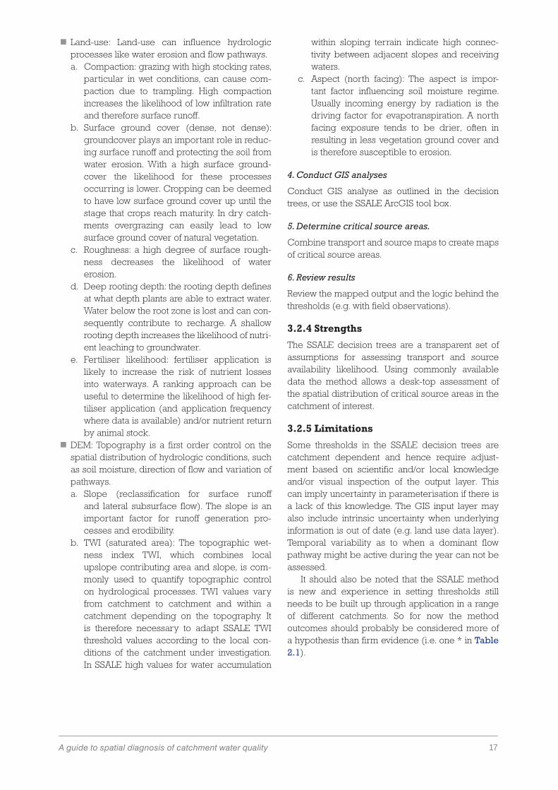
� Land-use: Land-use can influence hydrologic processes like water erosion and flow pathways.a. Compaction: grazing with high stocking rates,
particular in wet conditions, can cause com-paction due to trampling. High compaction increases the likelihood of low infiltration rate and therefore surface runoff.
b. Surface ground cover (dense, not dense): groundcover plays an important role in reduc-ing surface runoff and protecting the soil from water erosion. With a high surface ground-cover the likelihood for these processes occurring is lower. Cropping can be deemed to have low surface ground cover up until the stage that crops reach maturity. In dry catch-ments overgrazing can easily lead to low surface ground cover of natural vegetation.
c. Roughness: a high degree of surface rough-ness decreases the likelihood of water erosion.
d. Deep rooting depth: the rooting depth defines at what depth plants are able to extract water. Water below the root zone is lost and can con-sequently contribute to recharge. A shallow rooting depth increases the likelihood of nutri-ent leaching to groundwater.
e. Fertiliser likelihood: fertiliser application is likely to increase the risk of nutrient losses into waterways. A ranking approach can be useful to determine the likelihood of high fer-tiliser application (and application frequency where data is available) and/or nutrient return by animal stock.
� DEM: Topography is a first order control on the spatial distribution of hydrologic conditions, such as soil moisture, direction of flow and variation of pathways.a. Slope (reclassification for surface runoff
and lateral subsurface flow). The slope is an important factor for runoff generation pro-cesses and erodibility.
b. TWI (saturated area): The topographic wet-ness index TWI, which combines local upslope contributing area and slope, is com-monly used to quantify topographic control on hydrological processes. TWI values vary from catchment to catchment and within a catchment depending on the topography. It is therefore necessary to adapt SSALE TWI threshold values according to the local con-ditions of the catchment under investigation. In SSALE high values for water accumulation
within sloping terrain indicate high connec-tivity between adjacent slopes and receiving waters.
c. Aspect (north facing): The aspect is impor-tant factor influencing soil moisture regime. Usually incoming energy by radiation is the driving factor for evapotranspiration. A north facing exposure tends to be drier, often in resulting in less vegetation ground cover and is therefore susceptible to erosion.
4. Conduct GIS analyses
Conduct GIS analyse as outlined in the decision trees, or use the SSALE ArcGIS tool box.
5. Determine critical source areas.
Combine transport and source maps to create maps of critical source areas.
6. Review results
Review the mapped output and the logic behind the thresholds (e.g. with field observations).
3.2.4 Strengths
The SSALE decision trees are a transparent set of assumptions for assessing transport and source availability likelihood. Using commonly available data the method allows a desk-top assessment of the spatial distribution of critical source areas in the catchment of interest.
3.2.5 Limitations
Some thresholds in the SSALE decision trees are catchment dependent and hence require adjust-ment based on scientific and/or local knowledge and/or visual inspection of the output layer. This can imply uncertainty in parameterisation if there is a lack of this knowledge. The GIS input layer may also include intrinsic uncertainty when underlying information is out of date (e.g. land use data layer). Temporal variability as to when a dominant flow pathway might be active during the year can not be assessed.
It should also be noted that the SSALE method is new and experience in setting thresholds still needs to be built up through application in a range of different catchments. So for now the method outcomes should probably be considered more of a hypothesis than firm evidence (i.e. one * in Table 2.1).

18 Landscape Logic Technical Report No. 20
3.2.6 Complementary methods
SSALE decision tree outcomes can be compared with results from spatial ‘snapshot’ surveys (e.g. EC, nutrients, and other parameters). The SSALE decision trees and their thresholds typically draw on the understanding generated by the Initial spatial conceptual modelling.
ReferencesBuczko U, Kuchenbuch RO (2007) Phosphorus indices as risk-
assessment tools in the U.S.A. and Europe—a review. J. Plant Nutr. Soil Sci., 170, 445–460.
Caruso BS (2001) Risk-based targeting of diffuse contaminant sources at variable spatial scales in a New Zealand high country catchment. Journal of Environmental Management 63, 249–268.
Drewry JJ, Newham LTH, Greene RSB (2007) An index-based modelling approach to evaluate nutrient loss risk at catch-ment-scales. p. 2326-2332. In: Oxley, L. and Kulasiri, D. (Eds) MODSIM 2007 International Congress on Modelling and Simulation. Modelling and Simulation Society of Australia and New Zealand, December 2007.
Melland R, Smith A, Waller R (2007) Farm Nutrient Loss Index. An index for assessing the risk of nitrogen and phosphorus loss for the Australian grazing industries. User Manual for FNLI Version 1.18. Department of Primary Industries, Ellinbank, Victoria.
Morgan RPC (1986). Soil Erosion and Conservation. Essex, 298 pp.
National Committee on Soil and Terrain (2009) Australian Soil and Land Survey, Field Handbook. Third Edition. CSIRO pub-lishing, Collingwood. 246 pp.
Newham LTH, Jakeman AJ, Letcher RA, Heathwaite AL, Smith CJ and Large D (2002) Integrated water quality modelling: Ben Chifley Dam Catchment, Australia. p. 275-280. In: Integrated Assessment and Decision Support, Proceedings of the First Biennial Meeting of the International Environmental Modelling and Software Society, June 2002.
Sharpley AN, Weld JL, Beegle DB, Kleinman PJA, Gburek WJ, Moore Jr PA, Mullins G (2003) Development of phosphorus indices for nutrient management planning strategies in the United States. J. Soil Water Cons. 58, 137–152.
Strobl RO, Robillard PD, Shannon RD, Day RL, McDonnell AJ (2006) A water quality monitoring network design methodology for the selection of critical sampling points: Part I. Environmental Monitoring and Assessment 112, 137–158.

19A guide to spatial diagnosis of catchment water quality
3.3 Spatial ‘snapshot’ surveysA spatial ‘snapshot’ survey, also referred to as lon-gitudinal or synoptic sampling, is used to obtain information about the spatial location of point and non-point sources within the catchment. During a period of stable base flow the river system is sampled at every confluence providing a longitu-dinal profile of water quality (Grayson et al. 1997). The timing of sampling means the method is not suitable for estimation of relative contributions to annual load exports from the catchment, as these occur mainly during storm events. The base flow period is often, however, a critical time from an eco-logical health perspective. In addition, the chemical composition of a stream at any point reflects the combined impact of several factors such as geology, climatic conditions and land use in its contributing catchment area (Close and Davies-Colley, 1990). In the geochemistry literature, these snapshot surveys have been used with a range of statistical techniques to identify relationships between these factors and stream water quality (e.g. Close and Davies-Colley 1990, Wayland et al. 2003, Fröhlich et al. 2008).
In the context of a spatial catchment diagnosis, the snapshot survey can be used to explore the fol-lowing questions:1. From where in the catchment are nutrients and
sediments exported? Do the snapshot survey results verify areas identified as potential critical source areas by the initial conceptual mod-elling (Section 3.1) and spatial source area likelihood estimation (Section 3.2)?
2. Do the snapshot survey results show any other unexpected increases or decreases in concen-trations along the streams and tributaries?
3. Do the snapshot survey results allow grouping of sampling sites that suggest they are affected by similar processes?
3.3.1 Inputs
� Spatially referenced water quality data: z TN, TP, Turbidity (required for minimal analysis) z NO3–N, NH4–N, TN, DRP, TP, TSS, Turbidity, EC (desired)
z Above + NO2–N, DON, PN, PP (optional – depending on analysis questions)
� Water flow measurements at locations of sam-pling (optional)
3.3.2 Monitoring design
Sampling locations should be chosen so as to rep-resent changes in the landscape along the length of the river and its tributaries. Tributaries should be sampled as close as possible to the conflu-ence with the main stream, but out of the zone of
influence from the main stream (e.g. from flood events). To carry out a numerical longitudinal analy-sis of relative loads the main stream should also be sampled before and after the confluence. Local land use issues should be taken into account, e.g. sam-pling upstream of cattle crossings or road culverts. Choice of sampling locations may also be influ-enced by practical considerations such as access (public vs. private land), and stability of and access to the stream bank. If initial conceptual modelling and/or a spatial source area likelihood estimation has been carried out, representative sites of the dif-ferent zones should be sampled and stream sections draining potentially critical source areas should be captured by sampling both up- and down-stream of them.
Sampling should ideally capture some of the seasonal differences, e.g. both a summer and a win-ter snapshot survey. To reduce impact of sampling or lab errors it is useful to repeat sampling at least once.
3.3.3 Tools � Sampling equipment and protocols � Excel or alternative spreadsheet tool � Several statistical packages provide tools for for-mal, statistical cluster analysis. See Kaufman and Rousseeuw (2005) for an introduction to methods.
3.3.4 Data analysisSnapshot data is often presented as follows (exam-ples from the worked example for the Duck River catchment in Section 4.4).
Maps
Maps provide a quick overview of how concen-trations vary (at a certain point in time) within the catchment (between different zones, or between main channel and tributaries). This allows for easy comparison with e.g. initial conceptual modelling and maps of critical source areas as derived from the spatial source area likelihood estimation. Studies reported in the literature use maps as follows:
� with sampling locations represented by circles of different colour or size representing different concentration classes (e.g. Figure 4.11, Figure 4.12) (Works only with limited number of classes.)
� with sampling locations represented by small cir-cles and results written alongside
� with results printed in sampling locations and the stream network reflected by straight line segments (i.e. more like a diagram) (Particularly useful when a quantitative analysis of relative contributions at each confluence is car-ried out.)

20 Landscape Logic Technical Report No. 20
� with stream segments coloured accord ing to results from the sampling point (To be reliable, this requires a large number of sampling points that are representative of the stream segments.)
Transects
Transects are useful for more in-depth study of changes up- or downstream and allows for easy parallel plotting of results for different constituents or combining results from different times. Transects can be used with:
� results plotted as a function of distance up- or downstream along main channel (e.g. Figure 4.13)
� tributary results indicated in the same graph or in a second graph underneath (with junction with main channel as the distance up/downstream)
� results plotted as bar graphs in up- or downstream order with flux loads (if available) added as line graph or presented separately.
Derived data
Derived data like the fraction of NO3/TN or TN/TP, etc. can be useful, depending on issues being considered.
Cluster analysis
Cluster analysis can be used to evaluate whether sampling sites fall into ‘natural’ groups; this can be carried out informally or using formal techniques:
� Plot results for all sites (main channel and tributaries) as bar graphs, box-whisker (if multiple sampling times) or using symbols instead of bars, but with gridlines shown (e.g. Figure 4.15). Visually identify groups of sites with similar results by comparing graphs for the different constituents.
� Plot three-dimensional scatter diagrams or ternary diagrams (triangles) for three constituents at once and visually identify groups of sites with similar results.
� Create minimum variance dendograms (‘trees’) using a formal cluster analysis technique (Kaufman and Rousseeuw, 2005; see e.g. Figure 4.17)
� Create principal component ordination diagrams using formal principal component analysis.
3.3.5 Interpretation
1. Establish concentration distributions for key nutrients
Are there any areas within the catchment that stand out due to having very high or low stream concen-trations? Are there seasonal differences in these patterns?
� Determine suitable concentration classes from a bar graph, box-whisker graph, or graphs like in
Figure 4.15 and then plot the results on maps. � Evaluate whether the concentration patterns correspond with land use, soils or land form, or the zones identified in the Initial spatial conceptual modelling.
� Evaluate whether any spatial patterns or seasonal differences are consistent with the hydrologic interpretations of different parts of the catchment (see step 4).
2. Longitudinal analysis
Are there gradual or sudden changes along the transects of different rivers and creeks in one or more of the water quality parameters (nutrients, TSS, turbidity, EC, DOC)? Changes can relate to inflows of water with higher or lower concentrations, or be due to chemical or biological reactions converting e.g. one form of nitrogen to another or consuming or adsorbing nitrogen and effectively taking it out of the water column.
� Can the changes be ascribed to contributions from tributary streams or drains?
� Could there be biological or chemical reactions producing or consuming particular forms of the nutrients, or settling out of suspended sediments in the stream?
3. Relative loads
Where export of nutrients or sediments to another water body (e.g. wetland, dam, or estuary) is an issue, it is important to establish relative loads, as concentration data alone can give a skewed picture. It should, however, be stressed that these loads only reflect the continuous and relatively small contri-butions during baseflow conditions, while most of the annual loads are typically contributed during events. Nevertheless, from the point of view of eco-logical health the low flow period can be a critical time for rivers as well as receiving water bodies.
� If possible, obtain flow measurements at a few key locations to establish relative loads.
4. Identify zones with similar water quality issues
Looking at the range of water quality parameters (speciated nutrient concentrations, relative proportions of different forms, TSS, turbidity, EC, DOC, pH, etc) are there clusters of sites that observe similar water quality characteristics? (See example in Figure 4.16)
� The combination of high TP and high TSS sug-gests surface runoff and erosion processes may be active
� High nitrate, but low TP, may suggest subsurface transport is more dominant
� A sudden increase in EC could relate to influx from groundwater, or from a point source (e.g. animal or human waste).

21A guide to spatial diagnosis of catchment water quality
3.3.6 Strengths
� Quick, spatially extensive overview of rela-tive concentration levels in different parts of the catchment.
� Together with Initial spatial conceptual mod-elling this provides a very effective first identification of parts of the catchment that may be contributing more than others.
� When multiple measures (speciation of nutri-ents, EC, DOC) are jointly studied, hypotheses on pathways or origins can often be formed.
3.3.7 Limitations
� Unless flow is measured at each sampling point (a time consuming task), only concentration dif-ferences are measured, which only provides a partial picture of relative load contributions. Measurement of flow at a few key locations is recommended.
� The method is only suitable for stable base flow conditions, and hence does not capture event flow contributions from different parts of the catchment. The relative event flow contribu-tions may be different from the relative base flow contributions.
� Measures that are highly variable in time, even under stable flow conditions, are difficult to inter-pret using snapshot surveys.
� As the snapshot surveys typically rely on single sample analyses, any sampling or laboratory errors can complicate the interpretation or even provide a false interpretation. It is useful to repeat the snapshot survey at least once under simi-lar seasonal conditions (e.g. two winter and two summer snapshots) to enable checking for con-sistency of observed patterns.
3.3.8 Complementary methods
� Snapshot surveys can be used to confirm hypoth-eses set by Initial spatial conceptual modelling (Section 3.1) and spatial source area likelihood estimation (Section 3.2).
� High frequency monitoring (Section 3.5) can provide a temporal interpretation of the condi-tions during the snapshot survey.
� Where the snapshot survey suggests a particular origin (e.g. because of co-location with land use, or an influx of groundwater) isotope or tracer analyses are useful to confirm these hypotheses.
ReferencesClose ME, Davies-Colley RJ (1990) Baseflow water chemistry
in New Zealand rivers 2. Influence of environmental factors. New Zealand Journal of Marine and Freshwater Research 24, 343-356.
Fröhlich HL, Breuer L, Frede HG, Huisman JA, Vaché KB (2008) Water source characterization through spatiotemporal pat-terns of major, minor and trace element stream concentrations in a complex, mesoscale German catchment. Hydrological Processes 22, 2028-2043.
Grayson RB, Gippel CJ, Finlayson BL and Hart BT (1997) Catchment-wide impacts on water quality: the use of ‘snap-shot’ sampling during stable flow. Journal of Hydrology 199, 121-134.
Kaufman L and Rousseeuw PJ (2005) Finding groups in data: An introduction to cluster analysis. Wiley, New Jersey.
Wayland KG, Long DT, Hyndman DW, Pijanowski BC, Woodhams SM, Haack SK (2003) Identifying relationships between base-flow geochemistry and land use with synoptic sampling and R-mode factor analysis. Journal of Environmental Quality 32, 180-190.
22 Landscape Logic Technical Report No. 20
3.4 Event monitoringEvent monitoring refers to sampling of water quality during events at a temporal frequency that cap-tures the event in as much detail as possible. This is typically done using ‘auto-samplers’ which allow automated collection of water samples. The sam-ples are brought to a laboratory for analysis. In-situ analysers can also be used for event monitoring; they are discussed in Section 3.5.
Event monitoring has been used in many stud-ies to quantify nutrient export rates during events and explore controlling factors (Hawdon et al. 2007; Bainbridge et al. 2006; Vink et al. 2007). The analy-ses typically require information on discharge at the same time scale. The combination of concentration and discharge data can sometimes also provide insights into processes that govern the event export. It can, for example, help form hypotheses on the pathways by which the nutrients may have reached the stream (Heathwaite et al. 1989, Holz 2010).
3.4.1 Inputs
Event based samplers or ‘auto-samplers’ allow unat-tended, automated collection of water samples. These samplers can be set up for a range of tem-poral sampling intervals, either using fixed time intervals or sampling in response to stage height (discharge-weighted sampling). It can be set up to collect single samples or collect multiple samples into larger bottles (time or discharge weighted).
3.4.2 Monitoring design
Event monitoring is usually located at catchment or sub-catchment outlets, in locations suitable for parallel monitoring of discharge. Event based moni-toring may be suitable for monitoring at several key locations in the catchment and then provide a spatial assessment of sources during storm events to complement similar information from the spatial snapshot surveys for base flow conditions (Section 3.3).
3.4.3 Tools
Depending on the volume of data, data manage-ment systems can be used as outlined in section 3.5.2. With small amounts of data, spreadsheets offer a valid alternative for data organisation, stor-age, validation and analysis.
3.4.4 Data analysis
Depending on the scope, data analysis can include one and/or a combination of the methods used for high frequency and snapshot sampling (Sections 3.3.4 and 3.5.4).
3.4.5 InterpretationInterpretation would have many parallels to that of high frequency monitoring data, except that the length and density of data record is likely to be more limited. See Section 3.5.5 for details. When used spatially with a number of event samplers at key locations in the catchment, the analysis would focus on timing of start of events, relative magnitude of events in different locations (when converted to loads using discharge measurements), and dif-ferences in temporal event dynamics of different constituents. Timing and distribution of rainfall within the catchment would need to be taken into account.
3.4.6 StrengthsA wider variety of water quality parameters can be analysed in the lab compared to high frequency analysers, which are typically restricted in the num-ber of parameters they can analyse. The numbers of parameters is, however, restricted by the capac-ity of the sampling bottles and the volume needed for lab analysis. Costs associated with event sam-plers are less than for high frequency analysers. Event samplers are in principle easy to install and have low maintenance requirements, although sam-ples do need to be collected and when refrigeration is required (see 3.4.7 below) installation is more complicated.
3.4.7 LimitationsEvent samplers require samples to be collected and taken to the laboratory for analysis. They can only take a restricted number of samples (i.e. typically 24 samples maximum) before requiring sample collection. This can limit the monitoring of complete events (rising limb and falling limp of the hydro-graph) and/or during periods with high and closely spaced, consecutive events over a longer period. As a consequence, either more frequent site visits or a switch to lower temporal resolution of sampling is required.
Preservation of samples can be critical. Biological and physiochemical changes can con-tinue to occur in the sample bottles and may even be enhanced when exposed to higher temperatures and/or light. Samples should, therefore, ideally be collected immediately after the event and/or being refrigerated and kept dark. Refrigeration usually requires access to mains power and securing of the instrumentation is preferable. Generally event sam-ples, especially of nitrogen and phosphorus, face the same issues that may affect the quality of the results as manually collected samples (Harmel et al. 2009), e. g. risk of deterioration during transport and sample storage and uncertainties associated with lab analysis routines.
23A guide to spatial diagnosis of catchment water quality
3.4.8 Complementary methods
Event based monitoring may be suitable for moni-toring at several key locations in the catchment and then provide a spatial assessment of sources during storm events (to complement similar information from the spatial snapshot surveys for base flow con-ditions (Section 3.3). One would probably first carry out the baseflow Spatial ‘snapshot’ surveys and the Initial spatial conceptual modelling, and from that choose locations for event monitoring to check rel-ative contributions from different zones to the total export load.
The relative value of event monitoring and high frequency monitoring depends on the questions one is trying to answer. It is, therefore, important to consider their role within the spatial catchment diagnosis. High frequency monitoring usually pro-vides more scope for process interpretations, although this depends on the scale of application. The instruments are also still quite costly. Event monitoring using auto-samplers is often cheaper, but there is a limit to the number of samples that can be taken and the samples need to be collected and analysed in a laboratory.
ReferencesBainbridge Z., Brodie J., Lewis S., Duncan I., Post D., Faithful J.,
Furnas M. (2006). Event-based Water Quality Monitoring in the Burdekin Dry Tropics Region 2004/2005 Wet Season. Australian Centre for Tropical Freshwater Research. Report, pp. 83.
Harmel R.D., Smith D.R., King K.W., Slade R.M. (2009). Estimating storm discharge and water quality data uncertainty: A software tool for monitoring and modeling applications. Environmental Modelling & Software 24:832-842.
Hawdon A., Keen R., Kemei J., Vleeshouwer J., Wallace J. (2007). Design and Application of Automated Flood Water Quality Monitoring Systems in the Wet Tropics, CSIRO Land and Water Science Report 49/07. pp. 31
Heathwaite AL, Burt TP, Trudgill ST (1989) Runoff, sediment, and solute delivery in agricultural drainage basins: A scale-depen-dant approach, p. 175-190, In: Regional Characterization of Water Quality, IAHS publication no 182.
Holz GK (2010) Sources and processes of contaminant loss from an intensively grazed catchment inferred from patterns in discharge and concentration of thirteen analytes using high intensity sampling. J. Hydrol. 383, 194-208.
Vink S., Ford P.W., Bormans M., Kelly C., Turley C. (2007). Contrasting nutrient exports from a forested and an agricul-tural catchment in south-eastern Australia. Biogeochemistry 84:247-264.
24 Landscape Logic Technical Report No. 20
3.5 High frequency monitoringHigh temporal frequency monitoring allows the observation of in-stream nutrient concentrations at the same timescale as hydrologic measure-ments. Three types of high frequency monitoring instruments can be distinguished: wet chemistry analysers, ion selective electrodes and UV/Vis spec-trophotometers. Depending on the system chosen, the measurement interval can be as small as a cou-ple of minutes to less than an hour (Bende-Michl and Hairsine, 2010). The high frequency measure-ments allow study of the ‘true’ pattern of nutrient dynamics under a variety of hydrologic conditions. These dynamics would usually go undetected by nutrient monitoring strategies using lower sampling frequencies (e.g. weekly, monthly).
Analysis of high frequency monitoring data spec-ifies exactly when and how nutrients and sediments are exported from the catchment, and the condi-tions under which this happens. This knowledge enables improved nutrient and sediment export load estimation. The combination of concentra-tion and discharge data can, however, also provide insights into processes that govern catchment scale water quality responses. It can, for example, help form hypotheses on the type of sources and the pathways by which the nutrients may have reached the stream (Heathwaite et al. 1989, Jordan et al. 2005., Holz 2010).
3.5.1 Inputs
� Monitoring of nutrients at a high temporal fre-quency at the catchment outlet (required)
z Measured species typically include TN, TP, NO3–N, NH4–N and PO4–P
z Temporal resolution of nutrient measurements (minutes – 1 hour)
z Data need to be checked for quality (e.g. removal of erroneous data points)
� Discharge data (hourly) (desired) � Rainfall data (hourly) (desired) � Additional monitoring at tributary outlets or particular areas of interest within the catch-ment (desired for establishing direct cause-effect relationships, between e.g. particular land use management systems in response to climatic drivers).
3.5.2 Monitoring design
High frequency monitoring is usually applied at catchment or sub-catchment outlets, in locations suitable for parallel monitoring of discharge. Some high frequency monitoring instruments could be used temporary at key locations in the catchment and then provide a spatial assessment of sources
during storm events to complement similar infor-mation from the spatial snapshot surveys for base flow conditions (Section 3.3).
3.5.3 Tools
Data organisation and cleaning
Due to the large amount of time series data gath-ered by high frequency monitoring, tools for data handling, such as database management systems, are recommended. These systems have the capa-bility to store, administer, clean and documentation observational data. In our work we encountered four major sources of errors in the high frequency data: (i) values above and below the detection limit, (ii) outliers caused by interferences (sudden spikes), (iii) drifts due to instrument cleaning issues (slow acceleration over time) and data losses and miss-ing values due to analyser malfunction (data gaps). Software products that work on database manage-ment systems can provide routines to identify, and remove those erroneous values.
Data analysis
Depending on the type of data analysis visual and statistical methods can be applied using the in-built functions of a spreadsheet (e.g. Excel) and/or statis-tics software (e.g. R, Mathlab).
3.5.4 Data analysis
Visual-graphical and descriptive statistical analyses are the first steps in exploring high frequency moni-toring data:
� Graphical analysis for long time series: Plot nutri-ent and discharge data as a function of time (providing a first impression of seasonal nutrient distribution)
� Graphical and descriptive statistical explora-tion of storm events (a response to rainfall in the catchment) and pollution events (that may be unrelated to discharge or rainfall)
z Determine the duration of events (from when discharge first increases until the next rise in the hydrograph or when flow reaches pre-event levels)
z Perform descriptive statistical analysis for each event: – Maximum, minimum, average, stan-
dard deviation for discharge and nutrient concentrations
– Time to reach maximum discharge and maximum nutrient concentration
– Maximum, minimum and average con-centration change over the duration of the event and/or until reaching maximum concentration.

25A guide to spatial diagnosis of catchment water quality
– Calculate ratios between inorganic nutri-ent species and totals (e.g. PO4–P:TP, NO3–N:TN)
z Perform graphical analysis for each event: Examine discharge-concentration relation-ships by plotting hysteresis effects: Categorise storm events according to hysteresis loop characteristics (direction and shape) (see e.g. Haygarth et al. 2004, Evans and Davies 1998)
z Examine relationships between storm events, rainfall and discharge characteristics, calculate – Amount of rainfall and discharge for hydro-
logic events – Discharge coefficients and the antecedent
wetness index can be used to assess event based wetness conditions
� Graphical and statistical exploration of the dry weather period: Examine the frequency distribu-tion of hourly concentrations for a series of days through for example box plots.
3.5.5 Interpretation
Combinations of the above analyses can be used to explore a number of questions. For example:
Is there a nutrient problem of significance and which nutrient species contribute(s) to the problem?
� Examine the time series data of the different con-stituents, as well as the ratio between inorganic nutrient species and totals to determine what is present and when:
z Which nutrient species dominate(s) through-out the year or during particular seasons or events?
z Are nutrients mostly present in inorganic form or particulate and/or dissolved organic form?
� Examine whether there are consequences for in-stream ecology or ecology of the receiving water body.
z How do maximum values and their frequency or duration compare to water quality guide-lines1 or biological effects data?
Is it a point source or a diffuse source?
� Examine the time series data of the different con-stituents during stable flow periods:
z Concentration spikes occurring over a short period (attaining a maximum within up to ~10
1 Note that high frequency data cannot be directly compared with water quality guidelines obtained from the 20th and 80th percentiles of monthly monitoring data, e.g. the ANZECC default trigger values.
hours) in the absence of a change in discharge may be indicative of a point source as reported for example by Jordan et al. (2005) (see also Figure 4.21).
� For the low period, examine box plots of hourly concentrations:
z In-stream biological activity causes regu-lar diurnal patterns of nutrient concentration fluctuations (Scholefield et al. 2005), but some-times they can also be related to point sources (Jordan et al. 2005).
� Diffuse sources are typically producing con-centration peaks of greater duration occurring concurrent with increases in discharge.
Where particulate material is concerned, is it mainly an in-stream source?
� Examine the time difference between the con-centration and discharge peaks.
z A large peak of particulate nutrients prior to the peak discharge during the first or first few events after a period of hydrologic inac-tivity points to a readily available source. This could be in-stream mobilisation (McDowell & Sharpley 2001)
z To determine the type of in-stream sources (e.g. deposited material or bank erosion) requires further analysis (e.g. geochemical analysis, mapping of river bank erosion).
Does the data suggest temporal change in sources and pathways?
� Examine event based statistical and graphical analysis results (concentration and discharge relationships, maximum and average nutrient concentration per event etc.)
z If event peak nutrient concentrations decline over time (seasonal time-scale) while the mag-nitude of event discharges remains similar this can be indicative of source depletion and/or a change in dominant contributing pathway (see e.g. Figure 4.18).
z Within event relationships between con cen tration and discharge (e.g. concentra-tion-discharge hysteresis loops) can relate to source depletion, transport limitations or a change in dominant contributing pathways. Examples of this type of interpretation can be found in e.g. Haygarth et al. (2004), Evans and Davies (1998).
26 Landscape Logic Technical Report No. 20
3.5.6 Strengths � Defining the nutrient species contributing to the catchment constituent export and the frequency distribution of peak concentrations of these nutri-ent species.
� Ecological risk analysis (cross disciplinary appli-cation): frequency distribution of particular nutrient threshold levels, nutrient exposure rates, diurnal riverine biogeochemical cycling
� Catchment scale nutrient management: accurate nutrient load estimation
� Understanding catchment responses: providing hypotheses on dominant sources and pathways. Note that as monitoring occurs at a catchment or subcatchment outlet the strength of the evi-dence is a function of the catchment scale. In smaller or more uniform catchments hypotheses will be stronger than in larger or heterogeneous catchments.
3.5.7 Limitations
� Currently only a limited number of nitrogen and phosphorus species can be analysed (totals and inorganic species). This limits interpreta-tion of biogeochemical processes, especially if dissolved organic forms are present. Filtering systems for longer term unattended deployment (> 3–4 days) are still under development.
� High cost: initial outlay and ongoing maintenance costs. A high qualified/skilled person for main-taining the system is desirable.
� Wet chemistry analysers require chemicals for the analysis (an additional cost) and some of these are hazardous.
� Ion selective electrode systems also use chemi-cals for calibration. They typically have a higher detection limit and require frequent recalibration.
� UV/Vis spectrophotometers are currently limited to nitrate as the only nutrient.
� Cost often precludes multiple sampling locations, limiting the ability to identify spatial nutrients and sediment sources.
� Reliability: a number of the instruments are com-plex and malfunction can occur often and due to various reasons (hardware failure, operating errors)
� Sufficient data management effort is required (data retrieval, storage, cleaning, documentation)
3.5.8 Complementary methods
� High frequency monitoring can provide a context and design parameters for speciated monitoring undertaken during Spatial ‘snapshot’ surveys. It can also provide further insights into seasonal differences observed in snapshots surveys.
� In return snapshot surveys provide a spatial con-text for the high frequency monitoring.
� Where high frequency monitoring provides hypotheses about catchment response and/or dominant sources or pathways, it can be checked to what extent this is consistent with the initial conceptual modelling.
� If the high frequency monitoring leads to hypoth-eses about the origins or pathways of sediments or nutrients, isotope and/or tracer analyses may be used to verify these.
� High frequency monitoring may inform ecologi-cal studies of responses to nutrient exposure.
ReferencesBende-Michl U. Hairsine PB (2010). A systematic approach to
choosing an automated nutrient analyser for river monitoring. Journal of Environmental Monitoring., 12, 127-134.
Evans C, Davies TD (1998) Causes of concentration/discharge hysteresis and its potential as a tool for analysis of episode hydrochemistry. Water Resources Research 34, 129-137
Haygarth P, Turner BL, Fraser A, Jarvis S, Harrod T, Nash D, Halliwell D, Page T, Beven K (2004) Temporal variability in phosphorus transfers: classifying concentration-discharge event dynamics. Hydrology and Earth System Sciences 8, 88-97.
Heathwaite AL, Burt TP, Trudgill ST (1989) Runoff, sediment, and solute delivery in agricultural drainage basins : A scale-dependant approach, p. 175-190, In: Regional Characterization of Water Quality, IAHS publication no 182.
Holz GK (2010) Sources and processes of contaminant loss from an intensively grazed catchment inferred from patterns in discharge and concentration of thirteen analytes using high intensity sampling. J. Hydrol. 383, 194-208.
Jordan P, Arnscheidt J, McGrogan H, McCormick S (2005) High-resolution phosphorus transfers at the catchment scale: the hidden importance of non-storm transfers. Hydrology and Earth System Sciences 9, 685-691.
McDowell RW, Sharpley AN (2001) A comparison of fluvial sediment phosphorus (P) chemistry in relation to location and potential to influence stream P concentrations. Aquatic Geochemistry 7, 255-265.
Scholefield D, Le Goff R, Braven J, Ebdor L, Long T, Butler M (2005) Concerted diurnal patterns in riverine nutrient concentrations and physical conditions. Science of the Total Environment 344, 201– 210.

27A guide to spatial diagnosis of catchment water quality
3.6 Isotope and tracer analysesIsotope and tracer analyses can be used to identify the origins of nutrients and sediments and/or where the water that carries them came from. Knowing the latter is often useful as it may indicate the pathway along which sediments and nutrients have travelled to the stream (but not always!). These methods draw their strength from conservative or predictable behaviour of constituents in the water and isotopes of the water or the constituents. Some commonly used methods include:
Natural geochemical tracers, such as alkalinity, Si, Ca, Na, Cl, and TOC. These have been used in a number of studies (e.g. Soulsby et al 2003) mainly in conjunction with End Member Mixing Analysis (EMMA). They require that all possible end-members – different sources of water in a catchment – can be identified and sampled and that their geochemical compositions are sufficiently distinct. The analysis requires careful analysis as sometimes solutes can be picked up by water, especially in surface runoff and shallow subsurface flow, which may then confuse the results (Kendall et al. 2001). Analysis for geochemical tracers can be done by most water quality laboratories.
Stable isotope tracers that have often been used in catchment studies include the isotopes of water (18O, 2H) and those of solutes (NO3, PO4, SO4 – 15N, 18O, 34S) and sediments or particulate material (e.g. 15N, 13C, 34S, 87Sr) (see Kendall and McDonnell (1998) for examples). Isotopes are forms of an element that have different numbers of neutrons (but all isotopes of an element have the same number of electrons and protons). Stable isotopes are isotopes that are not radioactive. Many different sources of nutrients have distinctive isotope ratios (expressed by d). See for example Figure 3.5 which shows the typical d18O and d15N values for a range of origins of nitrate. Many different processes (e.g., denitrification, nitrification) change the isotope ratios of the reactants and products (fractionation), but often in predictable ways. The existence and extent of the specific processes can, therefore, often be identified by measurement of the isotope ratios of the product and/or residual reactant (see e.g. the arrow indicating the direction of change with denitrification). While 18O, 2H, 15N, 13C, and 34S are all commonly analysed in many isotope laboratories, techniques for measuring isotopes of specific solutes (e.g. 15N and 18O of nitrate) are more specialised. The latter technique is, for example, not yet available in Australia. Note that these studies focus on natural abundance of the isotopes, rather than adding enriched isotopes.
Fallout (e.g. 137Cs, 210Pb) and lithogenic radio-nuclides 226Ra have been used to trace sediments. As with the other tracers – different sediment ori-gins are characterised by different isotope ratios. E.g. 137Cs is the product of above-ground nuclear weapons testing in the 1950–1970s and often has a maximum slightly below the surface (Wallbrink et al. 2003). It can, therefore, be used to estimate the contributions from cultivated topsoils and subsoils. ‘Composite fingerprints’, comprising a range of different diagnostic properties (geochemical trac-ers and isotopes) is also often applied (Collins and Walling 2002).
Radon (222Rn) an odourless and colourless radio-active noble gas that occurs naturally in air, in water, and in rocks and soil is often used pinpoint the loca-tion of groundwater –surface water interactions (see e.g. Cook et al. 2003).
A range of other tracers have been used as well. All methods are characterised by a forensic type approach. They typically require a working hypothesis that can be tested using targeted mea-surements. Used that way, they can however provide powerful evidence.
3.6.1 Inputs
Inputs depend on method used. It is often important that end-members are sampled and also that any variability in time is captured with repeat sampling.
3.6.2 Data analysis
This depends on the method used. Bar graphs, box-whisker graphs, three-dimensional scatter diagrams or ternary diagrams (triangles) are often useful, as are cluster analysis techniques and principal com-ponent analysis.
3.6.3 Interpretation
Interpretation of tracer data is often like solving a puzzle. Usually interpretation of measurements is not straight forward, and requires an understanding of the many interactions that can occur in the sys-tem. However, see Section 4.6 for a few examples.
3.6.4 StrengthsStrengths of isotope and tracer analyses are in identifying origin or pathways of nutrients and sedi-ments. When the problem is properly framed, the lines of evidence these analyses provided are often quite strong.
3.6.5 LimitationsAnalysis methods and in particular interpretation of data usually requires specialist input. Analysis costs can also be high.

28 Landscape Logic Technical Report No. 20
3.6.6 Complementary methodsIsotope and tracer analyses are typically carried out after a conceptual model of the catchment function has been formed using initial spatial con-ceptual modelling and spatial ‘snapshot’ survey results have been interpreted. They require work-ing hypotheses in order to frame the problem and target sampling.
ReferencesColllins AL and Walling DE (2002) Selecting fingerprint proper-
ties for discriminating potential suspended sediment sources in river basins. Journal of Hydrology 261, 218-244.
Cook PG, Favreau G, Dighton JC, Tickell S (2003) Determining natural groundwater influx to a tropical river using radon, chlorofluorocarbons and ionic environmental tracers. Journal of Hydrology 277, 74-88.
Kendall C, McDonnell JJ (1998) Isotope tracers in catchment hydrology. Elsevier, Amsterdam.
Kendall C, McDonnell JJ, GU W (2001) A look inside ‘black box’ hydrograph separation models: a study at the Hydrohill catch-ment. Hydrol. Process. 15, 1877–1902.
Soulsby C, Rodgers P, Smart R, Dawson J, Dunn S (2003) A tracer-based assessment of hydrological pathways at differ-ent spatial scales in a mesoscale Scottish catchment. Hydrol. Process. 17, 759–777.
Wallbring PJ, Martin CE, Wilson CJ (2003) Quantifying the contri-butions of sediment, sediment-P and fertiliser-P from forested, cultivated and pasture areas at the landuse and catchment scale using fallout radionuclides and geochemistry. Soil & Tillage Research 69, 53–68.
Figure 3.5: Typical ranges of d18O and d15N of nitrate from different origins (diagram courtesy of C. Kendall).

29A guide to spatial diagnosis of catchment water quality
4.1 DescriptionThe Guide to Spatial Diagnosis of Catchment Water Quality was developed while working on a case study in the Duck River catchment in north-west Tasmania. As part of this case study we developed, trialled and refined a number of methods. Findings from this study are used to illustrate some of the methods covered in this guide.
The Duck River catchment is located in north-west Tasmania and drains into Duck Bay at the town of Smithton. The catchment (area of approximately 542 km2) comprises three major landform components all of which dip to the sea from south to north. A flat low-lying plain is the central feature with the Duck River meandering across the plain. Uplifted blocks of rolling low hills with broad crests occur to the east and west of the plain (Figure 4.1). The Duck River provides the main drainage, although Deep Creek and its associated reservoir, Lake Mikany, provides the water supply for Smithton. The case study focussed on the Duck River above the tidal zone.
Rainfall received in the Duck River catchment increases from south to north. At the coast average annual rainfall is just over 900 mm/yr whilst at the southern edge of the catchment rainfall is in the order of 1500 mm/yr (rainfall at Forest is ~1000 mm/yr, at Irishtown ~1200 mm/yr, at Edith Creek ~ 1300 mm/yr). Rainfall is winter dominant, with over two
4. Duck River catchment case study
Figure 4.1: Duck River catchment (including Deep Creek and Scopus Creek, which drain directly into Duck Bay) and its location in Tasmania. Scotchtown monitoring station indicated by «.
thirds falling between the start of April and the end of October.
The distribution of soils in the Duck River catchment is shown in Figure 4.2a. Much of the catchment has not been surveyed and the map shown is an interpretation based on 1:25,000 geological mapping and local soil knowledge (Cotching and Cresswell, 2010, in prep).
Land use in the Duck River catchment is a mix of dairy farming, a significant portion being irrigated, grazing dry stock, cropping, plantation forestry, and native vegetation. Catchment land use is shown in Figure 4.2b. This map is an updated and enhanced version of land use mapping conducted by the Tasmanian Department of Primary Industries and Water (S. Broad, pers.comm).
The following sampling and analysis methods were applied in the Duck River catchment case study:
� Initial spatial conceptual modelling � Spatial source area likelihood estimation � Spatial ‘snapshot’ surveys (2 summer, 2 winter) � Geochemical analyses (targeted) � Radon analyses (targeted) � Nitrate isotope analyses (targeted)
The geochemical analyses and radon analyses were carried out to verify hypotheses about sources and pathways in selected parts of the catchment. A sub-set of the sites of the spatial ‘snapshot’ surveys was analysed using a dual 15N-18O nitrate isotope tech-nique. This was a pilot sampling as the technique is not yet available in Australia.

30 Landscape Logic Technical Report No. 20
Figure 4.2: Distribution of (a) soils and (b) land use in the Duck River catchment.

31A guide to spatial diagnosis of catchment water quality
Figure 4.3: Broad catchment disaggregation of the Duck River catchment.
4.2 Initial spatial conceptual modellingThe initial spatial conceptual model of the Duck River catchment is documented in a separate tech-nical report (Cresswell and Cotching, 2010). It provides background on the Duck River catchment, the available data and descriptions of the differ-ent zones within the catchment. Here we provide a brief summary to illustrate the different steps of the spatial conceptual modelling process outlined in Section 3.1.
1. Broad catchment disaggregation
For the development of the conceptual model the Duck River catchment was divided into seven different zones on the basis of expected nutrient sources and hydrological transport mechanisms (Figure 4.3) – thus reflecting soils and their distribution, land use and its distribution, landform, and local climate. For example, the hills and plains were separated on the basis of land form and the plains were then further divided into the Roger River Plains and Duck River Plains on the basis of soil type.
2. Hydrological interpretation
Descriptions for each of the zones are provided in Cresswell and Cotching (2010). Below examples from two of the zones:
Headwaters of the Duck and Roger Rivers zone
Due to the permeability of the soils, vertical water flow is likely to dominate in this zone. The permeable landscape can absorb much of the high rainfall, although surface water runoff is expected when soils reach field capacity or where surface compaction may have occurred (e.g. due to livestock). The hydrologic schematic for this zone shown in Figure 4.4.
Roger River and Duck River plains zones
The Hydrosols on the Roger River plains (often gleyed podzolic soils or humic gleys) are subject to prolonged periods of saturation. They are arti-ficially drained using open ditches and hump and hollow earthworks, root growth would otherwise be severely limited by lack of aeration. Saturation excess is the dominant runoff mechanism although artificial drainage will result in more vertical leach-ing and then subsurface lateral flow of water across to the drains (Figure 4.5). These Hydrosol soils may be saturated for up to 7 months of the year in this location. The wetness combined with extensive artificial drainage confers high hydrological connec-tivity across the plains and into the streams feeding Roger River. Nutrient pollution through surface and shallow subsurface water movement is likely, espe-cially given the high rainfall and propensity of the soils to exceed field capacity in late winter.

32 Landscape Logic Technical Report No. 20
The soils on the Duck River plains are subject to prolonged periods of saturation. Soils on Waratah, Hopeless, and Jones Plains plus parts of Mowbray Swamp have high groundwater levels leaving the soils wet for around 7 months per year. They are artificially drained using open ditches and hump and hollow earthworks. High water tables result in
Figure 4.4: HOST schematic for the Farnham silty clay loam representative of soils in the headwaters of the Duck and Roger Rivers zone.
high frequency of saturation and dominance of satu-ration excess runoff although artificial drainage will result in more vertical leaching and then subsurface lateral flow of water to the drains. The wetness com-bined with extensive artificial drainage confers high hydrological connectivity across the plains and into the streams feeding the Duck River.
Figure 4.5: HOST schematic for the drained soils in the Roger River and Duck River plains zones.
33A guide to spatial diagnosis of catchment water quality
3. Possible source areas and transport processes
Descriptions for each of the zones are provided in Cresswell and Cotching (2010). Below examples from two of the zones:
Headwaters of the Duck and Roger Rivers zone
� Nutrient transport into the groundwater in this zone is not thought likely to be a major issue due to the small area of livestock farming relative to native vegetation and plantation forestry, likely high soil P fixation, and the large amounts of dilu-tion coming from this high rainfall zone.
� The groundwater system is likely to be slow mov-ing, as evidence by the swamps on the plains to the north.
� Nutrient enrichment through surface water runoff is likely in areas of intensive landuse, especially given the high rainfall and propensity of the soils to exceed field capacity in late winter.
� However, runoff volumes per unit land area do not appear high as this is quite a permeable landscape and many local waterways appear ephemeral.
� The topography and lack of shallow water tables mean that for long time periods, large areas of the landscape are not hydrologically connected to the streams.
Duck River plains zone
� Nutrient pollution through surface water move-ment is highly likely on the plains given the wet soils, shallow groundwater tables and good rain-fall. Seasonal risk will be higher in late winter and early spring.
� Hump and hollow drainage will exacerbate the rapid removal of runoff water, ammonia has been
observed to move by this mechanism (Holtz et al. 2007).
� Open cut drains, used in conjunction with the hump and hollow system, will exacerbate the leaching of nitrate through vertical leaching and then lateral flow across to the drains (Holtz et al. 2007).
� Where these areas with strong hydrological con-nectivity to the river system support intensive dairying then both nutrient source and transport mechanism coincide, inferring high priority loca-tions for management intervention to prevent nutrient pollution.
4. Field verification
The above examples were taken from the initial conceptual model for the Duck River catchment (Cresswell and Cotching, 2010). The descriptions in this report already incorporated field observations of both the authors and of locals they consulted. Among other things, the field verification involved
� observations that streams from the eastern hills (e.g. Edith Creek, Allen Creek) had relatively small flow volumes when reaching the plains, but increased significantly in size within the plains zone, especially in winter. This allowed an assess-ment of likely relative contributions to catchment nutrient loads coming from the hills and plains;
� observations on hump and hollow drainage in the plains zones
� observations of erosion (limited), dairy laneways and livestock having direct access to streams (many places)
� observations of the presence of many in-stream dams in the eastern hills (Edith Creek, Allen Creek).

34 Landscape Logic Technical Report No. 20
4.3 Spatial Source Area Likelihood EstimationIn the application of the SSALE method to identify critical source areas in the Duck River catchment, we followed the steps outlined in Section 3.2 and made the following considerations:
1. Type of sourceAs there was little evidence of substantive gully ero-sion reaching the streams and bank erosion did not appear to occur at a large scale (Conceptual model, section 3.1), we determined that diffuse sources would be the main contributors to nutrient and sedi-ment exports.
2. Relevant decision treesOn the basis of the initial spatial conceptual model (Section 3.1) we considered the following transport pathways and nutrient/sediment sources (Table 4.1):
3. Reclassified inputsBased on the relevant decision trees for these pro-cesses from Appendix A, we reclassified input DEM, soils and land use information into layers with yes/no attributes using the following thresholds:
� Soils: Information was based on the soil survey of the Mowbray swamp (Hubble and and Bastick, 1995) and the Duck River catchment soil map prepared by Cotching and Cresswell (2010, in prep.; Figure 4.2).a. Low surface permeability : soils with low
surface permeability were defined by the saturated conductivity values (Ks) of the upper soil layer. We defined a low soil sur-face permeability by <5 mm/hr Ks (Ticehurst et al. 2007).
b. Profile permeability: the profile per-meability was determined by the saturated conductivity values (Ks) of soil profile layers other then the upper soil layer. We defined a high profile perme-ability as a saturated hydraulic conductivity < 100mm/hr Ks according to ASRIS (2005).
c. Erodibility: soils with a clay content between 9-30% and a silt content between 40-60% were used for a high likelihood of erosion (Morgan, 1986)
d. Impeding layer: a low hydraulic conductivity was characterised by < 5mm/hr Ks (Ticehurst et al. 2007).
e. Lateral transmissivity: if an indication of a pan or cemented layer existed in the soil profile layer.
� Landuse: a. Compaction: Grazing modified pastures and
cropping land uses were assumed to have a high likelihood of compaction occurring, either through tillage operation or through trampling by animal stock.
b. Surface ground cover: Cropping was deemed to have low surface ground cover up until crops reach maturity.
c. Roughness: Grazing modified pastures and irrigated cropping land uses were assumed to a high likelihood of having low surface roughness.
d. Deep rooting depth: Crops and grazing mod-ified pastures was assumed to have a high likelihood of low rooting depth.
e. Fertiliser risk: following consultation on typi-cal fertiliser application rates in the region we developed a fertiliser likelihood risk for high application rates. In the Duck River catch-ment the intensive dairy area in the flats were identified as having highest likelihood of fer-tiliser input (fertiliser application of about 65 kg P/ha/year and 300 kg N/ha/year) in addi-tion to high amounts of nutrients through stock return.
� DEM: a. Slope (reclassification for surface runoff and
lateral subsurface flow). We used a threshold of 2% in order to allow surface runoff erosion by water to occur (Ad-hoc-AG-Boden, 2005.)
b. TWI (saturated area): A value of TWI > 150 on sloping terrain indicated high lateral con-nectivity for the Duck River catchment. The value was defined by visual inspection of the results and is likely to be different in other catchments.
c. Aspect (north facing): Aspect values between 337.5 to 22.5 degrees were classified as north facing.
Transport pathway Source•Surface Runoff – Saturation Excess Flow
a. Infiltration Excess Flow•High likelihood through N and P fertiliser loss and return from cow/
sheep dropping
•Subsurface Run-off – Lateral Flow to Drains – Lateral Flow from Hills
•As above
•Nutrient Leaching to Groundwater •As above
•Surface Erosion by Water •As above and water erosion
Table 4.1

35A guide to spatial diagnosis of catchment water quality
4. GIS analysesWe then combined these layers in GIS analyses as outlined in the decision trees of Appendix A. This process is illustrated in Figure 4.7 for the surface runoff pathway.
5. Critical source areas The map with a high likelihood of saturated excess surface runoff is shown in Figure 4.8a, along with that of a high likelihood of P fertiliser source being available (Figure 4.8b). Combining these two maps shows that while the potential for transport is high in the whole of the central plains, the area likely to contribute to nutrient exports is more limited to that north from Edith Creek (Figure 4.8c). A similar derivation is shown for subsurface lateral flow in Figure 4.9.
6. Review of resultsThe SSALE output maps for the Duck catchment highlighted that (mostly northern) parts of the flat areas comprised a high likelihood for P loss. Two pathways were identified from these areas: satu-rated excess flow and subsurface flow to drains. Transport likelihood matched the earlier conceptual modelling outcomes.
Figure 4.6: SSALE decision tree for surface runoff with thresholds as set for the Duck River catchment.

36 Landscape Logic Technical Report No. 20
Figure 4.7: SSALE maps for surface runoff decision tree. As a result there is a high likelihood of saturated excess runoff and subsurface flow to drains in the flats dominating the transport pathways.
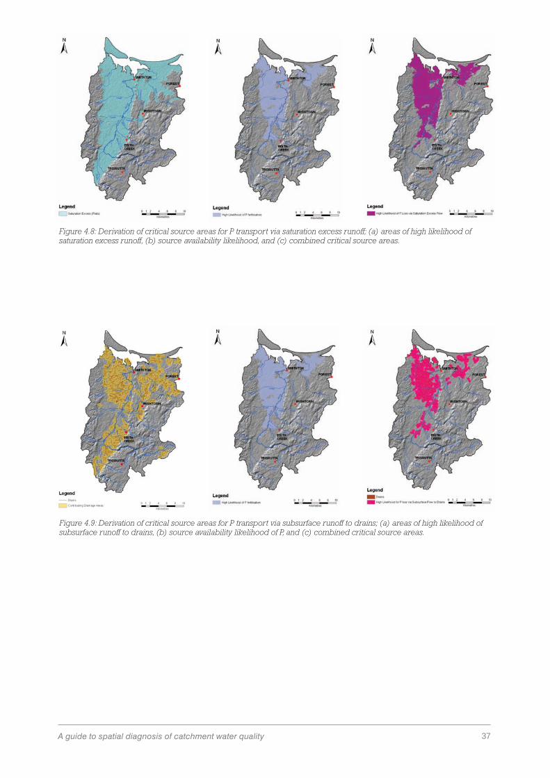
37A guide to spatial diagnosis of catchment water quality
Figure 4.8: Derivation of critical source areas for P transport via saturation excess runoff; (a) areas of high likelihood of saturation excess runoff, (b) source availability likelihood, and (c) combined critical source areas.
Figure 4.9: Derivation of critical source areas for P transport via subsurface runoff to drains; (a) areas of high likelihood of subsurface runoff to drains, (b) source availability likelihood of P, and (c) combined critical source areas.

38 Landscape Logic Technical Report No. 20
4.4 Spatial ‘snapshot’ surveysOver the course of the case study, four snapshot surveys were carried out with an expanding set of sampling sites (up to 50). These surveys were performed during stable base flow in summer and winter (Figure 4.10). Samples were analysed for different forms of nitrogen and phosphorus, EC, total suspended sediments, turbidity, pH and dissolved organic carbon on a subset of samples. A selection of results from the Duck River catchment case study is presented here to illustrate the information that can be extracted from spatial snapshot surveys. The presentation follows the same steps as outlined in Section 3.3:
1. Establish concentration distributions for key nutrientsMaps of the base flow concentrations of total phosphorus (Figure 4.11) and nitrate (Figure 4.12) confirmed the expectations from the initial conceptual modelling and critical source area analysis that transport and source likelihood are different in the plains and the hills of the Duck River catchment. High total phosphorus concentrations were predominantly found in the flats of the Duck River plains zone, whereas in the hills there were only a few ‘hot spots’ for total phosphorus and the location of these varied in time (Figure 4.15).
The snapshot surveys also showed clear
differences between summer and winter nitrate concentrations in most locations, except for a few sites in some streams just below the escarpment (Duck River, Spinks Creek, Birthday, Copper and White Water Creeks) that had year-around high nitrate concentrations (Figure 4.12).
2. Longitudinal analysisLongitudinal analysis of concentration changes in the Duck River showed a marked increase in nitrate at the escarpment, accompanied by an increase in EC and a decrease in dissolved organic carbon (DOC) (Figure 4.13). Tributaries flowing into the Duck River between these sites, could not explain the increase in EC. An influx of nitrate rich, high EC, but low DOC groundwater was suspected, which was consistent with the finding that the changes were more marked in summer. This was subse-quently analysed further using tracer and isotope analysis (see Section 3.6).
3. Relative loadsThe high concentration in e.g. Birthday Creek (Figure 4.12) still only delivers a small contribution to the overall load exported from the catchment due to its low relative flow volume contributed to the Duck River. Flows and loads in the Duck River increase significantly in the flats (confirming the initial conceptual model) (Figure 4.14).
Figure 4.10: Flow conditions (as measured in the Duck River at Scotchtown station) for the four ‘snapshot’ surveys (note different y-axis scales for summer and winter).

39A guide to spatial diagnosis of catchment water quality
Figure 4.11: Total phosphorus concentration observed during base flow in summer (Apr 09) and winter (Jun 09).
Figure 4.12: Nitrate concentration observed during base flow in summer (Apr ‘09) and winter (Jun 09).

40 Landscape Logic Technical Report No. 20
Figure 4.13: Duck River transects of nitrate, EC and DOC during the summer and winter snapshot surveys of 2009.
Figure 4.14: (Left) relative flows; (right) relative loads (June 2009 winter snapshot survey).

41A guide to spatial diagnosis of catchment water quality
4. Identify zones with similar water quality issuesSites DR1-DR7, DR47, DR49, DR50 in the Duck River Plains zone (Figure 4.15a) are all characterised by elevated TP levels (compared to sites elsewhere). The lower Geales Creek sites (DR2, DR50 and DR5 in downstream order) do, however, not have ele-vated DRP levels – these are uncharacteristically low (Figure 4.15b). On the other hand turbidity is extremely high at these sites at most sampling times (Figure 4.15c). This suggests that while
sharing many processes and characteristics with the rest of the Duck River Plains zone, the Geales Creek subcatchment, at least in the flats, has some other processes going on. This was explored fur-ther using geochemical analysis (see Section 3.6). Informal clustering of sites based on a range of water quality parameters (presented like in Figure 4.15) allowed identification different types of sites as shown in Figure 4.16. A formal statistical clustering analysis could provide input in this process (Figure 4.17).
Figure 4.15: Total phosphorus, dissolved reactive phosphorus and turbidity results from the four different spatial snapshot surveys.

42 Landscape Logic Technical Report No. 20
Figure 4.17: Example of statistic clustering of sampling sites Duck River catchment case study (clustering analysis courtesy of B. Henderson).
Figure 4.16: Informal clustering of sites: Green: High TP & High DRP & Med-High TSS & High NO3 in winter & elevated EC; Bright green: High TP, Low DRP, High TSS & High NO3 winter & Very high NH3 & Very high turbidity; Turquoise: Occasionally high or very high NH3, DRP, TSS, TP; Lavender: High NO3 winter & low NO3 summer & low TP; Orange: high NO3 winter and summer & low TP; Yellow: generally lower concentrations – or not (yet) clearly distinguishable.

43A guide to spatial diagnosis of catchment water quality
4.5 High frequency monitoringHigh frequency monitoring equipment was installed in the Duck River near the Scotchtown weir, the flow monitoring point of the Tasmanian Department of Primary Industries, Parks, Water and Environment, and upstream of tidal influences (see « in Figure 4.1). A few of the results are shown here.
Example 1: Graphic analysis of a seasonal time series
Comparison of the high frequency data with monthly routine sampling clearly demonstrates the additional information this data contains (Figure 4.18). Monthly routine sampling does not capture the nutrient dynamics; it misses how events evolve, the peak concentrations, and event duration. High
Figure 4.18: Observed TP (green symbols) and discharge (both hourly) during the high flow season of 2008, compared to monthly routine monitoring (red symbols).
Figure 4.19: Relative contributions of 20 different events during the 2008 high flow season (first five indicated by I – V) to (a) the total volume of discharge and (b) total P load.
0
500
1000
1500
2000
2500
3000
3500
4000
4500
15/05/2008 14/06/2008 14/07/2008 13/08/2008 12/09/20080
10
20
30
40
50
60
70TPDischarge
Con
cent
ratio
n [µ
g P
L-1
]D
ischarge [m3
s-1]
I II
III
IVV
I II
III
IVV
frequency data showed that the majority of nitrogen and phosphorus export was event driven. The first events of the high flow season carried relatively large loads of phosphorus despite the discharge peaks being low as a consequence of the landscape absorbing most of the rain. Later in the season the event peak nutrient concentrations gradually declined while the magnitude of event discharges remained similar. It is suspected this pattern is indicative of source depletion, however, at this large catchment scale this is difficult to prove without further investigations, e.g. including the study of rainfall patterns and soil moisture dynamics across the catchment. The data also demonstrated that the first 5–7 events during the 2008 winter carried about 50% of the total high flow load (Figure 4.19).
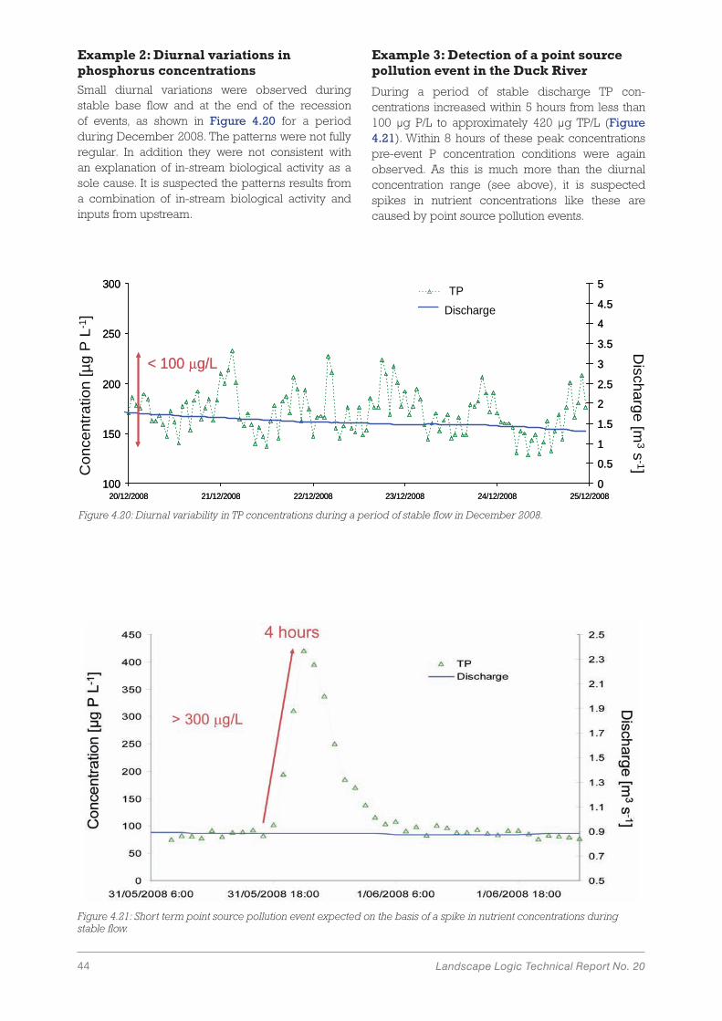
44 Landscape Logic Technical Report No. 20
Example 2: Diurnal variations in phosphorus concentrationsSmall diurnal variations were observed during stable base flow and at the end of the recession of events, as shown in Figure 4.20 for a period during December 2008. The patterns were not fully regular. In addition they were not consistent with an explanation of in-stream biological activity as a sole cause. It is suspected the patterns results from a combination of in-stream biological activity and inputs from upstream.
Example 3: Detection of a point source pollution event in the Duck River
During a period of stable discharge TP con-centrations increased within 5 hours from less than 100 µg P/L to approximately 420 µg TP/L (Figure 4.21). Within 8 hours of these peak concentrations pre-event P concentration conditions were again observed. As this is much more than the diurnal concentration range (see above), it is suspected spikes in nutrient concentrations like these are caused by point source pollution events.
Figure 4.20: Diurnal variability in TP concentrations during a period of stable flow in December 2008.
Con
cent
ratio
n [µ
g P
L-1
]D
ischarge [m3
s-1]
100
150
200
250
300
20/12/2008 21/12/2008 22/12/2008 23/12/2008 24/12/2008 25/12/20080
0.5
1
1.5
2
2.5
3
3.5
4
4.5
5TP [ppb]Q [m3/s]DischargeTP
100
150
200
250
300
20/12/2008 21/12/2008 22/12/2008 23/12/2008 24/12/2008 25/12/20080
0.5
1
1.5
2
2.5
3
3.5
4
4.5
5TP [ppb]Q [m3/s]DischargeTP
< 100 µg/L< 100 µg/L
Figure 4.21: Short term point source pollution event expected on the basis of a spike in nutrient concentrations during stable flow.

45A guide to spatial diagnosis of catchment water quality
4.6 Isotope and tracer analysesIn the Duck River catchment case study we applied geochemical analysis and isotope tracing to two issues that came up in the spatial snapshot survey (see Section 4.4):
� to test the hypothesis that high nitrate concentra-tions found in the Duck River and some creeks at the bottom of the escarpment came from high nitrate groundwater discharging as springs in these places; and
� to determine the reasons for the different P spe-ciation in Geales Creek.Geochemical analyses of cations, anions and
alkalinity were used to determine differences in water sources and radon analysis was used to check inflow of groundwater at the escarpment. In addition, to explore the value of the dual d15N-d18O nitrate isotope technique we carried out a pilot sampling of 15 samples in winter (August 2009) followed by a second pilot of 13 samples in sum-mer (March 2010). The aims of the pilot samplings were to establish whether or not isotope signatures from different locations in the catchment were dis-tinguishable, whether any land use impacts would show up (in particular animal dairy waste) and whether the spring samples would have a separate signature.
In relation to Geales Creek, we collected extra samples at the time of the second summer spatial snapshot survey and analysed these for alkalinity, chloride, sulphate, iron, manganese and silicate.
High nitrate concentrations at the escarpment.During both the winter and summer snapshot surveys high nitrate concentrations were found in Spinks, Birthday, Copper and White Water Creeks and the Duck River at the bottom of the escarpment (Figure 4.12). Significant changes in EC and DOC in the Duck River between DR25 (above escarpment) and DR20 at the bottom of the escarpment were also observed (Figure 4.13). The increase in EC could not be explained by inflows from Faheys and Lairds Creeks, which both had lower EC readings (DOC was not measured in these creeks due to budget limitations). Combined with the finding that the changes were more marked in summer, this suggested the possible inflow of groundwater with high nitrate and EC and low DOC (see Section 4.4). When we explored this possibility with locals from the catchment, they pointed us to a spring on Birthday Creek. The Tasmanian Department of Primary Industries, Parks, Water and Environment also confirmed the presence of a large spring on the Duck River and anecdotal evidence on the internet suggested the presence of springs in the Copper Creek area.
Radon analysis confirmed the inflow of ground-water in the Duck River and Birthday Creek at the escarpment, where radon activity readings were clearly elevated (Figure 4.22). Radon activity read-ings in Spinks Ck at the escarpment were not elevated, nor at a site further upstream. Whitewater Creek and Copper Creek were not sampled.
Figure 4.22: Sampling sites of Mar 2010 2nd nitrate isotope pilot and radon activity measurements.

46 Landscape Logic Technical Report No. 20
Presentation of the geochemical data of the same samples in semi-Piper (ternary) diagrams shows that the samples separated into two groups (Figure 4.23): those influenced by springs at the escarpment, and others. As this included samples of two of the springs themselves, this provided con-vincing support for the above hypothesis of nitrate
rich groundwater flowing into the Duck River and a number of creeks at the escarpment. Data for Copper Creek and Whitewater Creek from the State of Rivers Report (DPIWE, 2003) confirmed these creeks were also spring fed with groundwater from the same or similar origin.
Figure 4.23: Semi-Piper diagrams: March 2010 samples with State of Rivers data (DPIWE, 2003) for Copper, Coventry and Whitewater Creeks (all affected by springs).

47A guide to spatial diagnosis of catchment water quality
Knowing that groundwater discharging as springs was the source of high nitrate concentrations at the escarpment provided us with information about the pathway this nitrate had taken (Table 2.1, Table 4.2), but did not tell us about the origin of nitrate. The area around Trowutta has been farmed for at least 80 years and we know from the initial conceptual modelling that the soils are very permeable and rainfall is high. Nitrate leaching over an extended period could have reached deeper groundwater layers. There are also areas of karst in the area, which may have allowed faster transport to the groundwater body. On the other hand it is also possible that the nitrate has a natural origin. Data from the nitrate isotope pilots were inconclusive on that front. Most samples fell into the range of d15N where fertiliser and soil mineralisation origins cannot be distinguished (Figure 4.24). Samples from sites close to the springs and the springs
themselves did not appear to have a different nitrate isotope signature. Other markers may need to be applied to explore the origin of the nitrate.
On the other hand the nitrate isotope analyses did show that three samples were affected by animal waste. This included a drain in the plains near Birthday Creek under dairy land use, and the creek itself downstream from this point. It demonstrated that while concentration levels at both sites in Birthday Creek (one upstream near the spring and one in the plains downstream of drains) were similar, the origin of their nitrate changed in the plains in winter due to contributions from farm drains. It should be noted that a similarity in constituent concentration between two sites (as shown here for Birthday Creek) can be deceptive as constituent loads may still have increased (or decreased) and hence it does not mean that there were no additional constituent sources.
Figure 4.24: Dual nitrate isotope data from the first pilot (Aug 2009).

48 Landscape Logic Technical Report No. 20
High ammonium and turbidity in the Geales Creek catchment.Geales Creek is in the lower part of the Duck River plains zone that the initial conceptual model describes as being at a significant risk of nutrient pollution due to the high connectivity of the land with the streams (drains and shallow groundwa-ter in winter). Like other sites in the lower parts of the plains, the snapshot survey samples are char-acterised by high nitrate, especially in winter, high total phosphorus (TP) and medium to high total suspended sediments (TSS) (See Section 4.4). In addition ammonia and turbidity are extremely high at the lower Geales Creek sites (up to 0.7 mg N/L ammonia compared with values around 0.1 mg N/L for other lower Duck River plains sites; up to 70 NTU for turbidity compared with values around 10 NTU for other lower Duck River plains sites). These find-ings on their own could suggest that the Geales Creek area is particularly affected by nutrient losses from its dairy land use – more so than other sites in this zone.
Delving deeper into the snapshot survey
data, however, highlighted that there were other processes that also affect water quality in the Geales Creek subcatchment. Unlike the other lower Duck River sites, phosphorus at the lower (plains) Geales Creek sampling sites consisted mostly of particulate P and the dissolved fraction (as measured by DRP) was very small. The observation of red iron staining along the creek (Figure 4.25) suggested that acid sulphate soil issues may play a role in this subcatchment. Additional analyses of the April 2009 summer snapshot survey confirmed the presence of very low chloride to sulphate ratios (an indicator of acid sulphate soil issues), although pH in Geales Creek did not appear to be affected (yet) (unlike e.g. Scopus Creek as documented in State of Rivers report (DPIPWE, 2003)), although this could also reflect timing of sampling (stable low flow, dry period).
The low DRP concentrations are probably linked to the formation of iron-phosphate complexes, which are likely the cause of the observed high turbidity. It is likely the high ammonia values are also linked to the acid sulphate soil chemistry.
Figure 4.25: Iron staining of Geales Creek.

49A guide to spatial diagnosis of catchment water quality
4.7 Putting it together – the spatial catchment diagnosisA summary of methods applied in the Duck River catchment case study is shown in Table 4.2 with strength of evidence these methods provided indicated by one or three asterisks. The full ‘diagnosis’ is presented in Table 4.3, but it should be kept in mind that the case study was not performed in response to an identified impairment or triggered by condition monitoring results. It was purely a study to trial different methods, although the catchment was selected with attention to observed nutrient levels (among the highest in Tasmania), likely land-use impacts, and the presence of a receiving water body with aquaculture industry (Cresswell and Lefroy, 2007).
As shown in this worked example from the Duck River catchment, initial conceptual modelling provided a first assessment of possible source areas and transport processes, and when these might be active (Section 4.2). The use of the GIS approach of the Spatial source area likelihood estimation provided a second line of evidence for potential critical source areas and more precise specification of their locations and processes they relate to (Section 4.3). The spatial snapshot surveys (Section 4.4) confirmed some of the findings from the earlier methods, but also identified some other locations with high nutrient concentrations. As the surveys included full nitrogen and phosphorus speciation this provided valuable information about the form of nitrogen and phosphorus in different locations of the catchment. Where there was a clear co-location of high concentration levels, land use and landscape position, these surveys enabled hypotheses about the origins of the sediments and nutrients to be formed. Natural geochemical and isotope tracers
were used to confirm some of these sources as well as pathways (Section 4.6). High frequency monitoring provided a detailed insight in both species form and timing, and allowed hypotheses concerning pathways and transport processes (Section 4.5).
Figure 4.26 illustrates three of the evolving ‘stories’ from the case study, based on material presented in the worked examples throughout this guide. It is clear that the initial conceptual modelling provided a solid basis for the final summary or diagnosis. From Figure 4.26 and Table 4.3 it is also evident that a detailed spatial snapshot survey, which includes not only speciation of nitrogen and phosphorus, but also additional water quality parameters, has a high information content. It provides a key to further, more targeted investigations. While it may be tempting to stick to the initial diagnosis supported by just one or maybe two lines of evidence, the targeted additional measurements or analyses can improve understanding dramatically. Any apparent contradictions faded away as the conceptual model of the catchment evolved.
The process of documenting the evidence in a table like Table 4.3 or a flow diagram like Figure 4.26 encourages one to consider the consistency between lines of evidence. If required, the evidence can also be checked for consistency by formulating the spatial catchment diagnosis as a number of hypotheses. Table 4.4 illustrates that for the case of the origin of nitrate in Birthday Creek. The apparent contradictory evidence from nitrate isotopes prompted the revision of the conceptual model, allowing mixing of sources to happen in the plains, especially in winter when drains are frequently connected with the creeks.
Table 4.2: Methods and their contribution of evidence to the ‘diagnosis’ of Duck River catchment water quality issues.
Method Constituent/form Origin Source
areas Pathways Timing
Initial Spatial Conceptual Modelling * * * * *
Spatial Source Area Likelihood Estimation *** *
Spatial ‘snapshot’ surveys *** * *** *
Geochemical analysis *** ***
Radon analyses ***
Nitrate isotope analyses ***
High frequency monitoring *** * * ***
* Some information or allowing hypotheses to be formed *** Detailed information, confirming hypotheses

50 Landscape Logic Technical Report No. 20
ReferencesAd-hoc-AG Boden (2005) Bodenkundliche Kartieranleitung,
Hannover. Germany.ASRIS (2005) Australian Soil Resource Information System.
Technical specifications. Version 1.5 October 2005, NJ McKenzie, DW Jacquier, DJ Maschmedt, EA Griffin and DM Broughon,
Cresswell HP and Lefroy EC (2007) Selecting catchments in Tasmania for the nutrient and sediment management project . Landscape Logic Technical Report No. 6.
Cresswell HP and Cotching WE (2010) Duck River catchment conceptual model. Landscape Logic Technical Report (in press).
DPIWE (2003) State of the River Report for the Duck River Catchment. Water Assessment and Planning Branch, Department of Primary Industries, Water and Environment, Hobart. Technical Report No. WAP 03/08.
Holz GK (2007) Montagu River catchment: intensive grazing, drainage and water quality. Final Report UT11673, Tasmanian Institute of Agricultural Research (71pp)
Hubble GD and Bastick C (1995). The Soils and Land Use of Mowbray Swamp and Bordering Heathland, North-West Tasmania. Divisional Report No. 122, CSIRO Division of Soils.
Morgan RPC (1986). Soil Erosion and Conservation. Essex, 298 pp.
Ticehurst JL, Cresswell HP, McKenzie NJ, Glover MR (2007) Interpreting soil and topographic properties to conceptualise hillslope hydrology. Geoderma 137, 279-292.

51A guide to spatial diagnosis of catchment water quality
Table 4.3: Summary of findings in the Duck River catchment case study
Method Constituent/form Origin Spatial source Pathway TimingInitial spatial conceptual modelling
Organic and inorganic dissolved and organic particulate forms of N and P are expected to dominate.
High levels of animal returns and fertiliser usage are expected to contribute to N and P exports.There is little evidence of substantive soil (sheet and gully) erosion reaching the streams. Bank erosion does not appear to occur at a large scale.
The two plains zones are the most likely sources of N and P to the overall catchment loads because of the high connectivity with drains and streams being co-located with potentially high source likelihood.
In the plains zones saturated surface runoff and subsurface flow to drains are the likely dominant pathways delivering N and P to the streams.
Saturated surface runoff and subsurface flow would occur once the whole landscape is has wet up. Most exports are therefore expected from mid- winter to early spring.
Spatial source area likelihood estimation
By combining transport potential with source availability, critical source areas for nutrient losses are identified to be in the northern part of the Duck River plains (from Edith Creek north). Most other areas either do not have the high source availability or the transport potential.
Saturated surface runoff and subsurface flow to drains were confirmed to be the dominant pathways by which N and P from critical source areas reach the stream network.
Spatial ‘snapshot’ surveys
At most sites Total phosphorus during base flow conditions is made up of both particulate and dissolved P. The lower Geales Creek sites are however characterised by very low dissolved P.Nitrate is the main component of Total Nitrogen during base flow conditions, with particulate N and dissolved organic N generally making up the difference and the contribution of particulate N being highly variable from sampling time to sampling time. Ammonium concentrations were high at the lower Geales Creek sites and occasionally at sites in dairy areas of the plains zones.
The combination of high winter base flow concentrations of nitrate, total phosphorus, medium to high total suspended sediments, and elevated ammonium concentrations and EC are found where land use is almost exclusively dairy.
The combination of high winter base flow concentrations of nitrate, total phosphorus, medium to high total suspended sediments, and elevated ammonium concentrations and EC are found in the northern parts of the two plains zones (from Birthday Creek north).
Year-around high nitrate concentrations are also found in some streams just below the escarpment (Duck River, Spinks Creek, Birthday, Copper and White Water Creeks). In all but Spinks Creek this is accompanied by high EC levels, suggesting there may inflows from springs. The contributions to total loads from these streams is, however, small compared with that of contribution coming from plains. It may, however, affect local aquatic health conditions.Informal clustering of sites highlighted different nature of the Geales Creek sampling sites situated in the plains, with these sites having very little dissolved reactive P, unlike the other lower plains sites. The Geales Creek sites also have very high ammonium levels and very high turbidity. Combined with observed red staining along this suggests acid sulphate soil issues.
Catchment-wide there is a significant increase in base flow concentrations in winter. Combined with higher discharge (visual observations, Edith and Duck river discharge measurements) this results in significantly higher loads in winter.
In a number locations along the escarpment, however, nitrate concentrations are equally high during summer and winter.
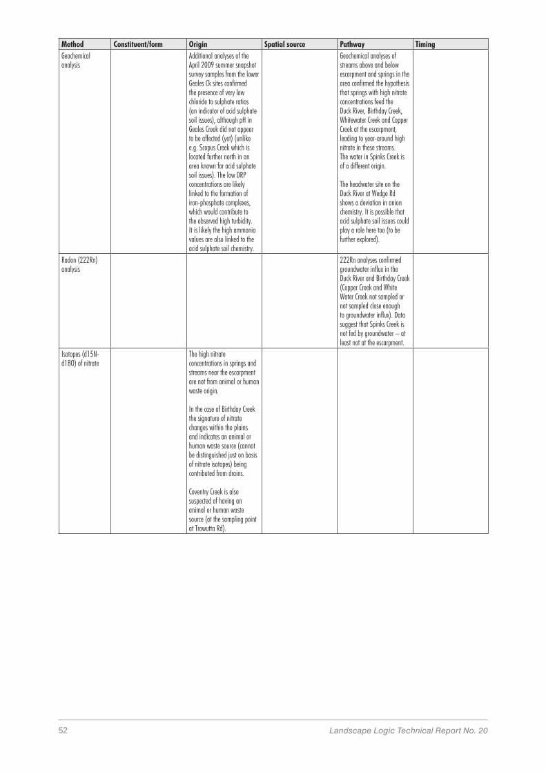
52 Landscape Logic Technical Report No. 20
Method Constituent/form Origin Spatial source Pathway TimingGeochemical analysis
Additional analyses of the April 2009 summer snapshot survey samples from the lower Geales Ck sites confirmed the presence of very low chloride to sulphate ratios (an indicator of acid sulphate soil issues), although pH in Geales Creek did not appear to be affected (yet) (unlike e.g. Scopus Creek which is located further north in an area known for acid sulphate soil issues). The low DRP concentrations are likely linked to the formation of iron-phosphate complexes, which would contribute to the observed high turbidity. It is likely the high ammonia values are also linked to the acid sulphate soil chemistry.
Geochemical analyses of streams above and below escarpment and springs in the area confirmed the hypothesis that springs with high nitrate concentrations feed the Duck River, Birthday Creek, Whitewater Creek and Copper Creek at the escarpment, leading to year-around high nitrate in these streams.The water in Spinks Creek is of a different origin.
The headwater site on the Duck River at Wedge Rd shows a deviation in anion chemistry. It is possible that acid sulphate soil issues could play a role here too (to be further explored).
Radon (222Rn) analysis
222Rn analyses confirmed groundwater influx in the Duck River and Birthday Creek (Copper Creek and White Water Creek not sampled or not sampled close enough to groundwater influx). Data suggest that Spinks Creek is not fed by groundwater – at least not at the escarpment.
Isotopes (d15N-d18O) of nitrate
The high nitrate concentrations in springs and streams near the escarpment are not from animal or human waste origin.
In the case of Birthday Creek the signature of nitrate changes within the plains and indicates an animal or human waste source (cannot be distinguished just on basis of nitrate isotopes) being contributed from drains.
Coventry Creek is also suspected of having an animal or human waste source (at the sampling point at Trowutta Rd).

53A guide to spatial diagnosis of catchment water quality
Method Constituent/form Origin Spatial source Pathway TimingHigh frequency water quality monitoring
During the first large event of winter dissolved P is the main component of Total P, but during subsequent events P is mainly in particulate form.
During base flow P is mostly in dissolved form.
Phosphorus spikes during low flow (rainfall independent) vary in their form, presumably depending on their origin.
The (semi)diurnal variations in nutrient concentrations seen during low flow are expected to be influenced by diurnal riverine transformation processes, but with inputs from upstream modifying these patterns.
Spikes seen during low flow (rainfall independent) are hypothesized to be due to point sources.
Analysis of the concentration patterns in conjunction with discharge patterns allows hypotheses to be formed on processes affecting individual events.
A large event late during winter shows a dilution effect of P.
Total P loads are highest in winter, but especially the first 5-7 events of winter. These were shown to contribute approximately half of the total winter event load in both 2008 and 2009.
These first large events are characterised by P concentration patterns that peak before the discharge peak. During subsequent events peak P concentrations coincide with the discharge peaks. Concentration patterns relative to discharge patterns suggest a switch from initially transport limited.
(Semi) diurnal variations in nutrient concentrations are seen during low flow (rainfall independent).
Occasional spikes in nutrient concentrations are seen during low flow (rainfall independent).

54 Landscape Logic Technical Report No. 20
Figure 4.26: Evolving ‘stories’ in the Duck River catchment case study and their implications.

55A guide to spatial diagnosis of catchment water quality
Table 4.4: Alternate hypotheses on the origin of nitrate in Birthday Creek and evidence
The origin of nitrate in Birthday Creek is due to: Dairy origin Groundwater origin
Initial spatial conceptual modelling: groundwater influx not considered, surface runoff and subsurface flow via drains from dairy land considered likely pathway and origin.
+ –
Spatial snapshot survey: map with concentrations of nitrate at both sites in Birthday Creek shows similar concentrations, suggesting nitrate levels were already high before entering dairy land use area
–a +a
Spatial snapshot survey: the combined analysis of multiple parameters provided strong suggestions of influx of high nitrate groundwater, potentially affecting both sites.
–a ++
Geochemical analysis: geochemistry of samples at both sites fitted with the cluster of samples from springs and spring-fed creeks.
– ++
Radon isotopes: radon analysis confirmed influx of groundwater near upstream site.
b ++
Nitrate isotopes: nitrate isotopes confirmed presence of nitrate from animal waste origin mixed in at the downstream site, especially in winter.
++ (downstream site)
0
Consistency of evidence
Initially appears inconsistent, but modified conceptual model of more than one source at down-stream site resolves this.
Supports
a) The fact that both sampling sites on Birthday Ck had similarly high nitrate concentrations could in absence of flow measurement be interpreted as supporting a common origin at the base of the escarpment. With flow measurements and a longitudinal analysis of loads, the story might, however, have been different.

56 Landscape Logic Technical Report No. 20
Appendix A: Spatial source area likelihood estimation (SSALE)
1. Consider whether the main sources in the catchment are point sources or diffuse sources.2. Choose the decision trees of relevance in the catchment under consideration:
Figure A.1: SSALE – Decision Tree for surface runoff, including infiltration excess runoff from hills and impervious areas as well as saturation excess flow from hills and slopes
Figure A.2: SSALE – Decision Tree for high likelihood of erosion by surface runoff

57A guide to spatial diagnosis of catchment water quality
Figure A.3: SSALE – Decision Tree for nutrient leaching to groundwater
Figure A.4: SSALE – Decision Tree for subsurface lateral flow

58 Landscape Logic Technical Report No. 20
Figure A.5: SSALE – Decision Tree for nutrient source (phosphorus)
Figure A.6: SSALE – Decision Tree for nutrient source (nitrogen)