a heuristic algorithm for determining the part set in a
TRANSCRIPT

University of LouisvilleThinkIR: The University of Louisville's Institutional Repository
Electronic Theses and Dissertations
5-2014
A heuristic algorithm for determining the part set ina powder-bed additive manufacturing machine.Sonja DiederUniversity of Louisville
Follow this and additional works at: https://ir.library.louisville.edu/etd
Part of the Industrial Engineering Commons
This Doctoral Dissertation is brought to you for free and open access by ThinkIR: The University of Louisville's Institutional Repository. It has beenaccepted for inclusion in Electronic Theses and Dissertations by an authorized administrator of ThinkIR: The University of Louisville's InstitutionalRepository. This title appears here courtesy of the author, who has retained all other copyrights. For more information, please [email protected].
Recommended CitationDieder, Sonja, "A heuristic algorithm for determining the part set in a powder-bed additive manufacturing machine." (2014). ElectronicTheses and Dissertations. Paper 345.https://doi.org/10.18297/etd/345

A HEURISTIC ALGORITHM FOR DETERMINING THE PART SET IN A
POWDER-BED ADDITIVE MANUFACTURING MACHINE
By
Sonja Dieder
Diplom-Kauffrau, AKAD, College of higher education Pinneberg, 2004
Master of Science, University of Louisville, 2010
A Dissertation
Submitted to the Faculty of the
J. B. School of Engineering of the University of Louisville
in Partial Fulfillment of the Requirements
for the Degree of
Doctor of Philosophy
Department of Industrial Engineering
University of Louisville
Louisville, Kentucky, USA
May 2014

© Copyright 2014 by Sonja Dieder
All rights Reserved


ii
A HEURISTIC ALGORITHM FOR DETERMINING THE PART SET IN A
POWDER-BED ADDITIVE MANUFACTURING MACHINE
By
Sonja Dieder
Diplom-Kauffrau, AKAD, College of higher education Pinneberg, 2004
Master of Science, University of Louisville, 2010
A Dissertation Approved on
February, 20 2014
by the following Dissertation Committee
______________________________________________
Dr. William E. Biles, Dissertation Director
_____________________________________________
Dr. Brent Stucker
______________________________________________
Dr. Gerald W. Evans
______________________________________________
Prof. James A. Leach

iii
DEDICATION
This dissertation is dedicated to the loving memory of my father
Wilhelm Dieder
And to my mother
Maria Dieder
My deepest gratitude goes to my father. He tried to teach me in Math when I was a young
girl with endless patience and without despairing ☺

iv
ACKNOWLEDGEMENTS
I would like to express my deepest respect and gratitude to my dissertation
director Dr. William Biles for developing and providing outstanding and constant support
from the original idea to the innovation. This dissertation study would not have been
possible without his patient guidance and enthusiastic encouragement of this research
work and during all these years in the program.
I would also like to thank Dr. Brent Stucker for his valuable support and advice in
the area of Additive Manufacturing. Special thanks to Dr. Gerald Evans for contributing
his extensive knowledge in Simulation and Decision Making. Great appreciation is also
offered to Professor James Leach for his excellent support during this dissertation work
and all the graduate school years. He taught accurately and repeatedly to build up a solid
foundation of Graphical Visualization for being in a position for this research work.
I would also like to thank Joseph Vicars for his assistance with a SolidWorks
model.
My grateful thanks are also extended to Mr. Timothy Gornet who assisted with
his excellent skills and advices of the build setup and the background knowledge of the
SLS machine. I would also like to thank Mr. Randall Storey and Dr. Nathan Johnson for
their technical support with infrastructure and software issues.

v
Particular thanks to Dr. Gail DePuy, Director of IE Graduate Programs, for
contributing her excellent knowledge in Foundations of Optimization and Experimental
Design in Engineering. She offered a great support during the program.
Special acknowledgement also goes to Peggy Sue Prater for her assistance with
regulations, as well as organizational, operational and personal matters over all the years
of that program.
I feel special gratitude for my beloved one around me for supporting me with
strong encouragement, motivation and patience in my ongoing process of profound
change. Also special thanks to my fellow student, Peter Brem for his friendship and for
sharing the general ups and downs that come along with this challenge.
In addition I would like to express my gratitude to Siemens AG and Nokia
Siemens Networks GmbH & Co. for the encouragement to pursue the Ph.D. Also my
special thanks to Hartmut Müller-Leitloff, Martin Lüst and Stephan Kalb for promoting
and motivating me and for providing advice and actions over a long time.

vi
ABSTRACT
A HEURISTIC ALGORITHM FOR DETERMING THE PART SET IN A
POWDER-BED ADDITIVE MANUFACTURING MACHINE
Sonja Dieder
February 20, 2014
The goal of this research is to develop a procedure for the placement of a priority
part into a planned build in a powder-bed additive manufacturing machine. Toward that
goal, a heuristic procedure was developed that seeks to maximize the revenue in a
scheduled build, subject to due-date constraints; i.e., all parts with the closest due date
will not only be included in the build, but will be placed near the bottom of the build.
Likewise, any part in the scheduled build that does not have an immediate due
date is a candidate for removal in order to accommodate a higher priority part, the order
for which arrives after the build is underway. The build volume for this experiment with
the SLS2500+ machine is 13-inch x 15-inch x 18-inch rectilinear container.
To achieve this optimization of the build, the experiment for this research
involved a penalty which is based on failure to meet the due date constraint.
The m parts in the build are placed such that are placed the highest priority parts,
including those with immediate due date constraints, are positioned near the bottom of
the build volume.

vii
The focus of this study is to determine which “unbuilt” parts x(i) will be removed
to make room for higher priority parts. Toward that end, each part is assigned a priority
p(i), i = 1, …,m until the build is full. If an order for a part having a higher priority
p(i)than any of the parts in the build, the procedure developed here seeks to replace at
least one of the parts in the scheduled build.
Hence, the dimensions of the lower priority parts are key, since the part that is
removed must provide sufficient space for the new part. Importantly, the enactment of the
procedure developed here takes place in real time, with little or no interruption of the
progress of the build.
The resulting Excel file will be sorted as to place the immediate items at the
bottom on the build. The solution is valid for a single and also for a multiple build.
Simulations of this heuristic procedure were shown to substantially increase the
revenue desired from the planned build by adding higher priority parts.

viii
TABLE OF CONTENTS
ACKNOWLEDGEMENTS ................................................................................... iv
ABSTRACT .......................................................................................................... vi
TABLE OF CONTENTS ..................................................................................... viii
LIST OF TABLES ................................................................................................ xi
LIST OF FIGURES .............................................................................................. xii
INTRODUCTION ................................................................................................. 1
LITERATURE REVIEW ...................................................................................... 2
2.1Rapid Prototyping vs. Additive Manufacturing ................................................... 2
2.1.1Fused Deposition Modeling (FDM) ............................................................ 4
2.1.2 Stereolithography Apparatus (SLA) ........................................................... 6
2.1.3D Printing (3DP) ...................................................................................... 8
2.1.4 Selective Laser Sintering (SLS) ............................................................... 12
2.1.4.1.Indirect Metal Selective Laser Sintering (IMSLS) ............................... 15
2.1.4.2.Selective Laser Melting (SLM) ......................................................... 15
2.1.5.Direct Metal Laser Sintering (DMLS) ...................................................... 23
2.2 AM Process and Supply Chain ................................................................. 25

ix
2.2 Genetic Algorithm .................................................................................. 40
2.3 Bin Packing Problem............................................................................... 43
RESEARCH APPROACH .................................................................................. 45
3.1 New Approach ....................................................................................... 45
3.2 Additional Literature Review ................................................................... 46
PART PACKING ................................................................................................ 52
4.1 The Selective Laser Sintering Machine SLS 2500+ .......................................... 52
4.2 The Part Set ................................................................................................. 55
4.3The Build Setup ............................................................................................ 55
4.4 The Bounding Box Problem .......................................................................... 57
4.5 Multiple Builds ............................................................................................ 66
REVENUE MAXIMIZATION ............................................................................ 70
5.1 Commercial Trends ...................................................................................... 70
5.2 Cost estimation ............................................................................................ 83
5.3Development of the Mathematical Model ........................................................ 88
OPTIMIZATION APPROACHES AND EXPERIMENTAL RESULTS .............. 93
6.1 Optimization Approaches ........................................................................ 93
6.1.1. MATLAB ............................................................................................ 94
6.1.2. LINGO ................................................................................................ 94
6.1.3. EXCEL Solver ...................................................................................... 97
6.2Experimental Results ................................................................................... 110

x
SUMMARY, CONCLUSIONS AND RECOMMENDATIONS ........................... 113
7.1 Summary ............................................................................................. 113
7.2 Conclusions ......................................................................................... 114
7.3 Recommendations for Future Work ........................................................ 114
REFERENCES ................................................................................................. 115
APPENDIX A: Part Catalogue .......................................................................... 118
APPENDIX B: MATLAB GA for Bin Packing ................................................... 153
APPENDIX C: LINGO model and solution ........................................................ 176
APPENDIX E: List of Abbreviations ................................................................. 223
CURRICULUM VITAE .................................................................................... 228

xi
LIST OF TABLES
Table 2.1 Common examples of AM techniques ..................................................... 4
Table 2.2 Summary Extrusion methods (Gebhardt, 2004) ........................................ 5
Table 2.3 Summary Stereolithography(Gebhardt, 2004) ........................................... 7
Table 2.4 Summary 3D Printing (Gebhardt, 2004) ................................................ 10
Table 2.5 Summary Selective Laser Sintering ....................................................... 16
Table 2.6 Checklist for additional purchase of components(Zäh, 2006) ................... 17
Table 2.7 Checklist for procurement of a system(Zäh, 2006) .................................. 20
Table 2.8 Lean and agile supply chain operators (Mason-Jones et al. 2000) ............. 30
Table 2.9 Strategic reasons for using RM for individual cases ................................ 31
Table 5.1 Excel overview of all parts, dimensions and Bounding Volume ................ 98
Table 5.2 Excel Columns for the Solver solution ................................................. 101

xii
LIST OF FIGURES
Figure 2.1 Fused Deposition Modeling(Gebhardt, 2004) ....................................... 5
Figure 2.2 Stereolithography(Gebhardt, 2004) ...................................................... 7
Figure 2.3 3D Printing(Junk et al., 2010) ............................................................. 9
Figure 2.5 Laser Sintering(Boillat et al., 2004) ................................................... 14
Figure 2.6 Product supply chain matrix (Fisher 1997) ........................................ 29
Figure 2.7 Modified production and supply chain matrix (Fisher 1997) ................ 30
Figure 3.1 Inputs, outputs and processes incl. in a product’s life cycle .................. 48
Figure 3.2 Inputs, outputs and the other side of economics: SALES ...................... 51
Figure 4.1 Major components of the SLS System ............................................... 53
Figure 4.2 Pause Build ..................................................................................... 54
Figure 4.3 Build Modify in the SLS 2500+ ........................................................ 54
Figure 4.4 Mouth tray as SolidWorks model ..................................................... 56
Figure 4.5 Build Setup from the Part Set ........................................................... 56
Figure 4.6 Build Setup from the Part Set with the main information ..................... 57
Figure 4.7 Procedure of finding out the minimum BB of a model ......................... 62
Figure 4.8 Bounding Box Kind ......................................................................... 63
Figure 5.1 AM allows for new business models .................................................. 71
Figure 5.2 AM can be more customer friendly .................................................... 71
Figure 5.3 AM can lead to USP ........................................................................ 72

xiii
Figure 5.4 Still some issues .............................................................................. 72
Figure 5.5 AM and business issues .................................................................... 73
Figure 5.6 Individual products from Shapeways marketplace ............................... 74
Figure 5.7 Overview Materialise ....................................................................... 77
Figure 5.8 Overview Twinkind ......................................................................... 78
Figure 5.9 RM supply chain instead of RP supply chain ...................................... 79
Figure 5.10 Scheme of the costing model ............................................................ 84
Figure 5.11 Production curve for the lever (LS) .................................................... 85
Figure 5.12 Cost Overview ................................................................................ 85
Figure 5.13 Screenshot from the Build Setup ....................................................... 86
Figure 5.14 Screenshot from the Build Setup – Part Info ....................................... 87
Figure 5.15 Screenshot from the Build Setup – Time Estimate ............................... 87
Figure 5.16 Screenshot Solver Parameter ........................................................... 102
Figure 5.17 Solution for a single build ............................................................... 103
Figure 5.18 Visual verification for the single machine solution ............................ 104
Figure 5.19 Visual verification for the single machine solution – information ........ 104
Figure 5.20 Solution for multiple machines – first part ........................................ 105
Figure 5.21 Solution for multiple machines – second part .................................... 106
Figure 5.22 Solution replacement of the parts..................................................... 107
Figure 5.23 Visual verificationfor replacement of the parts .................................. 108
Figure 5.24 Visual verificatiofor replacement of the parts – information ............... 108

1
CHAPTER 1
INTRODUCTION
Rapid Prototyping is the general heading about different procedures for the quick
production of pattern components constructed from digital data. In 2009 the F42
Committee on Additive Manufacturing Technologies (ASTM International) adopted the
term Additive Manufacturing (AM) for these procedures. The Technical Committee 261
standardized AM for ISO (International Organization for Standardization). Improvements
in the quality of the output from these machines have led to a higher quality, more precise
part – often equal to that needed for final products. Parts are now fabricated directly by
layer-by-layer deposition of material using three-dimensional Computer Aided Design
(CAD) data. In the powder-bed additive manufacturing process, a rastering infra-red laser
beam heats the surface of a powder bed to fuse the powder in a cross-section that matches
that of a prototype being replicated.
The bin packing problem can be described as follows: given a set of boxes of
different sizes, how should one pack them into containers of a given size, in order to use
a few containers as possible.
The objective of this research is to design m parts to a “build” with the possibility
that part way through the build one or more higher priority parts arrive. Which “unbuilt”
parts can be removed from the build to make room for the higher priority parts?

2
CHAPTER 2
LITERATURE REVIEW
This chapter gives an overview about Rapid Prototyping vs. Additive
Manufacturing and it’s technologies as well as Genetic Algorithms, Cutting and Packing
Optimization and a summary of research in that area so far.
2.1Rapid Prototyping vs. Additive Manufacturing
Rapid Prototyping (RP) can be defined as a process for rapidly creating a system
or part representation as a prototype or base model from which further models and
eventually the final product will be derived. The term Rapid Prototyping describe a
process of developing business and software solutions in a piecewise fashion that allows
clients to test ideas and provide feedback during the development process. In a context of
product development, the term RP was used widely to describe technologies which
created physical prototypes directly from digital data. However, the term RP overlooks
the basic principle of these technologies in that they can often fabricate final parts using
an additive approach.(Gibson et al., 2010) and now Additive Manufacturing is the
worldwide standard name for these processes in the technical community
(http://www.astm.org/COMMITTEE/F42.htm,
http://www.iso.org/iso/standards_development/technical_committees/other_bodies/iso_te
chnical_committee.htm?commid=629086)

3
ASTM defined a Standard Terminology for Additive Manufacturing
Technologies. The recent version F2792-12a includes terms, definitions of terms,
descriptions of terms, nomenclature, and acronyms associated with AM technologies in
an effort to standardize terminology used by AM users, producers, researchers, educators,
press/media and others.
The major terms in this dissertation will also complement with the official
definition of the Standard Terminology.
Standard Terminology:
“Additive Manufacturing (AM), – a process of joining materials to make objects
from 3D model data, usually layer upon layer, a opposed to subtractive manufacturing
methodologies.”
“Rapid Prototyping (RP), – additive manufacturing of a design, often iterative, for
form, fit, or functional testing, or combination thereof”.(ASTM International, 2012)
Additive Manufacturing first emerged in 1987, with Stereolithography (SL) from
3D Systems, a process that solidifies thin layers of ultraviolet (UV) light-sensitive liquid
polymer using a laser. The SLA-1 was the first commercially available AM system in the
world (Wohlers and Gornet, 2011).
In Rapid Prototyping, shapes are constructed not by ablation through turning or
milling, but rather the part arises through joining volume elements layer by layer. Based
on that explanation, Rapid Prototyping methods are also called “generative production
methods”.

4
Common examples of AM techniques are shown in Table 2.1 (Padhye and Deb,
2011)
Table 2.1 Common examples of AM techniques
Technique short cut
Fused Deposition Modeling FDM
Stereolithography SLA
3D printing 3DP
Selective Laser Sintering SLS
Direct Metal Deposition DMLS
2.1.1Fused Deposition Modeling (FDM)
Standard Terminology: “a material extrusion process used to make thermoplastic
parts through heated extrusion and deposition of materials layer by layer; term denotes
machines built by Stratasys, Inc”..(ASTM International, 2012)
Fused Deposition Modeling (FDM) was developed in the 1980s by S. Scott
Crump. The FDM process consists of having a heated, melted thread of plastic pass onto
a “build-platform” in a layer-by-layer fashion via an extrusion nozzle. The nozzle is
controlled by a mechanical “print head” and computer aided manufacturing software that
contains the final image of the product. Upon hitting the build platform, the liquid
solidifies and the platform lowers where the next layer of hot material is laid upon it. The
process continues until the product is complete(http://www.prototypepros.com/rapid-

5
prototyping/fused-deposition-modeling.fdm/). Table 2.2 gives a short summary
describing the FDM method.
Figure 2.1 Fused Deposition Modeling(Gebhardt, 2004)
Table 2.2 Summary Extrusion methods (Gebhardt, 2004)
Extrusion methods
Method Fusion of solid plastics (wire or block) in a heated nozzle. Layered
construct through extrusion. Solidification through cooling. Pillars
needed.
Materials Different kinds of plastic, partially nominally series identical (ABS
Acrylonitrile butadiene styrene, PPSF Polyphenylsulfone)
Advantages Higher mechanical and thermal loading capacity then

6
Stereolithography.
Disadvantages Rougher surfaces, lower level of detail then Stereolithography
2.1.2 Stereolithography Apparatus (SLA)
Standard Terminology:
“Stereolithography (SL), – a vat photopolymerization process used to produce
parts from photopolymer materials in a liquid state using one or more lasers to selectively
cure to a predetermined thickness and harden the material into shape layer upon layer.”
“Stereolithography Apparatus (SLA), – denotes the SL machines from 3D
Systems Corporation” (ASTM International, 2012).
Stereolithography was invented and patented in 1986 by Charles Hull of 3D
Systems Inc. (http://www.wikipedia.org). It is a method and apparatus for making solid
objects by successively printing thin layers of the ultraviolet curable material one on top
of the other.(http://www.3dsystems.com/news/25th-anniversary/) The material used is
liquid photo-curable resin, acrylate. Under the initiation of photons, small molecules
(monomers) are polymerized into large molecules. Based on this principle, the part is
built in a vat of liquid resin.(Yan and Gu, 1996). Table 2.3 gives a short summary of the
Stereolithography process.

7
Figure 2.2 Stereolithography(Gebhardt, 2004)
Table 2.3 Summary Stereolithography(Gebhardt, 2004)
Stereolithography
Method Local hardening of liquid monomer through UV radiation (laser,
lamp), pillar or support material is needed
Materials Epoxy resins, acrylates
Advantages High level of detail, very good surfaces
Disadvantages Lower mechanical and thermal loading capacity then Laser Sintering
and Extrusion techniques. Specialty resins for higher temperatures
available

8
2.1.3D Printing (3DP)
Standard Terminology: “the fabrication of objects through the deposition of a
material using a print head, nozzle, or another printer technology”.(ASTM International,
2012)
3D printing was invented by Prof. Emmanuel Sachs from Massachusetts Institute
of Technology (MIT). This technology uses ink-jet printing nozzles to jet binder droplets
onto solid powder surface. After one layer is formed, the next layer of powder is spread
on the former layer. By providing a linear nozzle array, the forming velocity can be
accelerated. 3D printing was commercialized by Soligen Corporation in the US in the
name of DSPC (Direct Shell Production Casting) used for manufacturing of ceramic
shells and cores for casting. Other similar machines are 3DP (Extruhone, US), and 3DP
(Z-Corp, US).

9
Figure 2.3 3D Printing(Junk et al., 2010)
3D printing needs no additional support, and can form an extensive range of
materials that can be bonded by available binders such as ceramics with binder, metals
with binder and polymers with binder. (Yan et al., 2009). Table 2.5 gives a summary of
3D printing technology.

10
Table 2.4 Summary 3D Printing (Gebhardt, 2004)
3D Printing
Method Injection of binder fluids in a powder bed. Mechanical load through
infiltrate. No pillars needed.
Materials Starch/Water, plaster-ceramic/water, metal
Advantages Rapid and cost-effective, cold process, color models possible
Disadvantages Minimal level of detail, rough surfaces.
Starch and plaster + infiltration: low loading capacity, undefined
mechanical properties
Actually iMaterialise offers a wide variety of 17 different materials and 70
possible color and finish combinations for 3D printing.

11
Figure 2.4 Materials for 3D printing (http://i.materialise.com/materials)
1. Polyamide
2. Alumide
3. Multicolor
4. High detail resin
5. Paintable resin
6. Transparent resin
7. ABS
8. Titanium
9. Stainless Steel

12
10. Silver
11. Gold
12. Prime gray
13. Brass
14. Bronze
15. Ceramics
16. High detailed stainless steel
17. Rubber-like
2.1.4 Selective Laser Sintering (SLS)
Standard Terminology:
Laser Sintering (LS), – “a powder bed fusion process used to produce objects
from powdered materials using one or more lasers to selectively fuse or melt the particles
at the surface, layer by layer, in an enclosed chamber”.
Selective Laser Sintering (SLS), – “denotes the LS process and machines from 3D
Systems Corporation”. (ASTM International, 2012)
In 1992, Selective Laser Sintering from DTM (now a part of 3D Systems) and the
Soliform Stereolithography system from Teijin Seiki became available. Using heat from a
laser, SLS fuses powder materials. The Soliform technology was originally developed by
DuPont under the Somos name and was subsequently licensed to Teijin Seiki for

13
exclusive distribution rights in parts of East Asia. Also in 1992, Allied Signal introduced
vinylether Exactomer resin products for SL. (Wohlers and Gornet, 2011)
The generative technology, Sintering, was invented at the beginning of the 90s. At
that time it was named as Laser Sintering, because all systems worked with a laser. For
differentiation to industrial Sinter methods and due to solidification only in selected
sections, the term Selective Laser Sintering (SLS) was more appropriate. In 2001 the
ARCAM machine was introduced which works with an electron beam instead a laser. In
2005 the Speed Part AB machine was introduced which works with an infrared emitter.
Based on those new technologies the generic name “Selective Sintering” or “Sintering” is
generally used. (Gebhardt, 2007)
In the SLS process, a rastering infrared laser beam heats the surface of a powder
bed to fuse the powder in a cross-section that matches that of a prototype being
replicated. The surface is then covered with another layer of powder and the cycle is
repeated. The current fused layer is bonded to that beneath to build up the 3D shape of a
part. (Berzins et al., 1996)
The obtained part has a rigid but porous structure. The loose powder can be
removed and recycled. Small powder particles tend to melt earlier and more completely
than big ones under the laser radiation. The surface tension of the droplets leads to the
accumulation of liquid phase at the contact points of the large, solid grains.
This process is called “the necking phenomenon” because the bonding between
the particles usually look like necks. (Boillat et al., 2004)

14
Figure 2.5 Laser Sintering(Boillat et al., 2004)
The EOS GmbH is manufacturer of layer manufacturing techniques (LMT).
These techniques, also sometimes referred to as solid freeform manufacturing (SFM) and
other names, enable physical parts to be manufactured directly from computer-aided
design (CAD) data, quickly and automatically. They stated that their machine EOSINT
(SLS) builds with a similar procedure to STEREOS (SLA), in that the part is built up
layer by layer on a platform by scanning a laser beam over the material surface. The
fundamental differences are that the material is in powder form and the solidifying
process is a thermally induced phase change rather than a chemical reaction. In principle
almost any fusible material can be used, but it has to be available with suitable surface
properties for recoating and optical and thermal properties matched to the laser radiation.
Suitable materials include thermoplastics and low-to-medium melting point metals. This
can be extended to other materials such as ceramics or high melting point metals.
(Behrendt and Shellabear, 1995)
The following process variants became known in Selective Laser Sintering:

15
• Indirect Metal Selective Laser Sintering (IMSLS)
• Selective Laser Melting (SLM)
2.1.4.1.Indirect Metal Selective Laser Sintering (IMSLS)
Indirect Metal Selective Laser Sintering (IMSLS) allows steel/bronze composite
parts to be made through a combination of selective laser sintering of a polymer coated
steel powder to create a “green” part, followed by furnace infiltration of the green part
with bronze. The resulting parts are fully dense functional components which can be
exploited for demanding engineering applications, such as injection moulding
tooling.(Zakaria and Dalgarno, 2010)
2.1.4.2.Selective Laser Melting (SLM)
Selective Laser Melting (SLM) has been developed driven by the need to produce
near full dense objects with mechanical properties comparable to those of bulk materials
and the desire to avoid lengthy post processing cycles. Polymers as well as metals can be
completely molten by a laser beam. The appellation Selective Laser Melting is reserved
for metallic materials.
In the ease of processing (e.g. laser absorption, surface tension and viscosity of
the liquid metal, etc.), all metals may be thought of as candidate materials; however, large
differences exist. For each new material, a process-window needs to be determined
experimentally in order to ovoid scan track instabilities (sphereodisation of the liquid
melt pool, also known as “balling”) and part porosity.
In recent years, the idea of full melting metal powders was explored, supported by
the continuously improving process parameters (smaller layer thickness, smaller spot

16
size, etc.), resulting in mechanical properties being much better than those of early time
selective laser sintered parts and comparable with bulk metal properties.(Kruth et al.,
2005a)
Table 2.5 gives a summary of SLS technologies.
Table 2.5 Summary Selective Laser Sintering
Selective Laser Sintering
Method Local fusing of powdered thermoplastic material, layer formation after
solidification. No pillars needed.
Materials Plastics (polyamide, polystyrene), metals, sands, ceramics
Advantages Plastics: high mechanical and thermal load then Stereolithography
Disadvantages Rougher surface, lower level of detail then Stereolithography
Sintering and melting can be used with all materials which behave like
thermoplastics. Therefore, Sintering provides a significantly wider variety of materials
then Stereolithography. The resultant components are mechanically and thermally
loadable. According to the material and application they can be used as a functional
model and often as the end product. Based on that fact, Sintering is the key to Direct
Tooling, (the direct manufacturing of tools and tool inserts) and also for Direct
Manufacturing, the generative production of end products.

17
Powder that has not been melted can be partially recovered and can be put back in
the process, mostly by mixing with unused powder. The recycling rate depends on the
degree of damage and lies in case of polyamide powders between 50 and 30% used
powder in the new construction process.(Gebhardt, 2007)
To help in the decision process for choosing the best application and the most
economical generative production process, there are two checklists available, one
checklist for additional purchase of components and the second checklist for procurement
of a system. Table 2.6 gives a checklist for selecting an SLS system.
Table 2.6 Checklist for additional purchase of components(Zäh, 2006)
Preconditions
1. Are STL, IGES, VDA data to manufacturers ready to submit?
2. Are 3D-constructions ready for transmitting?
4. Are all requirements of the components defined?
4.1 Roughness Level
4.2 Loading capacity
4.3 Heat resistance/acid resistance
4.4 Surface (coated, structured, etc.)
4.5 Accuracy
4.6 Number of parts

18
4.7 Additional requirements
5. Is the budget defined?
6. Is the technology predetermined?
7. Is the system operator detected?
Questions for determination of the right Rapid-Technology
1. Material properties required
2. Roughness Level required
3. Complexity of the parts
4. Size of the parts
5. Numbers of the parts
Definitions with the system operator
1. Shipping costs
2. Technology to apply
3. Component costs
4. Delivery deadline

19
5. Consequences for the delay of the delivery date
6. Dispatch type
7. Deadline for changes of the geometry
8. Costs of data preparation
Characteristics of the right manufacturer
1. Experiences with complying Rapid Technologies?
2. Customer references?
3. Component costs in the range of market level?
4. Established company inside Rapid area?
5. Advisory Service for possibilities and restrictions of appropriate
proceedings?
6. Manufacturer has appropriate resources (systems, employees)
7. Proximity of the manufacturer
8. New or regular supplier?
Table 2.7 gives a checklist to guide the procurement of an SLS system.

20
Table 2.7 Checklist for procurement of a system(Zäh, 2006)
Data Conditions
1. Is there an assessment realized by using STL data (mistake corrections,
supporting constructions, and slice-data-creation) technically usable in the
current software programs of the company?
2. Are there existing connections for data transfer in both directions from/to
the customer realized (internet connection, direct interconnections)?
4. Do the current computers have enough capacity for STL treatment?
5. Which software licenses for 3D-CAD proceedings are needed? Are there
existing connections for interchanging 3D data’s?
6. Which 3D data formats are required?
7. Are data storage and archiving ensured?
8. Are required measures for data security (DIN certification) introduced?
Workshop Conditions
1. Are media connections (power supply, cooling units, compressed air, or
protective gas) present?
2. Existing network connection (Ethernet)?

21
3. System requirements for temperatures/moisture/air purity can be fulfilled?
4. Are there special conditions for the facility environment (load capacity of
the ground, extraction units, vibration through other production plants)?
5. Existing space sufficient?(plant with periphery)
Accessibility to the plant ensured?
6. Existent storage room for building material sufficient?
7. Logistics assured? (transportation of components)
8. After treatment of components ensured?
9. Which periphery equipment for after treatment of components/material
preparation/material recycling is necessary?
Procurement of a system
1. Life cycle of plant components?
2. How many different materials can be used?
Are there different suppliers for the material?
3. What is the cost of building materials?
4. Are required quality of the component reproducible abided?
(surface, strength, dimensional accuracy, life cycle)

22
5. Are regulations or laws on hazardous material to apply?
6. Is the supply of spare parts ensured, also for the future?
7. Availability of service technicians?
8. Setup times (material handling, establishment of build jobs)?
9. Are the employees able to make maintenance by themselves?
10. Are maintenance contracts necessary?
11. Estimation of costs for service and maintenance?
12. Cycles and scope for needed Software/Hardware-Updates?
13. Stage of development for new materials?
14. Are safety data sheets for materials and for operation of the system
available?
Employees
1. Is operating staff available?
2. Is the training strategy scheduled?
3. Is there operating staff for possible after treatment for components
available?
4. Flexibility of the employees in case of working time?

23
2.1.5.Direct Metal Laser Sintering (DMLS)
Standard Terminology: “a powder bed fusion process used to make metal parts
directly from metal powders without intermediate ”green” or ”brown” parts; term denotes
metal-based laser sintering systems from EOS GmbH – Electro Optical Systems”.(ASTM
International, 2012)
The One-Stage SLS Process, also known under its commercial name Direct Metal
Laser Sintering (DMLS), is practiced with different materials. One of the main issues is
porosity. The One-Stage Liquid sintering is a portion of the practiced thermal sintering
with left over porosity. The material composition, the grain size and post treatment with
shot penning have helped to some extent to reduce this problem. The recently introduced
20 mµ metal powders bring a significant improvement in mechanical properties surface
quality and porosity of the productivity decreases strongly. (Levy et al., 2003)
The development with respect to functional, customized products will be
influenced in the future by achievable progress of the generative methods. New
technologies for layer manufacturing on plastic and metal basis, named Selective Laser
Sintering (SLS) and Selective Laser Melting (SLM), already known today economically
for Rapid Prototyping and Rapid Manufacturing, which are major contributions for the
flexibility of production technology. Through these methods it is possible to implement
complex functional components from several different plastics (polyamide, glass fiber-
reinforced plastics) and metal alloys (aluminum, titanium, steel alloy) in a short time
without complex CAD-CAM-interfaces. Typical examples for application are
biocompatible implants for the medical technology, mold inserts with internal cooling
channels for tool and mold construction as well as components for the aerospace industry.

24
The generation of control data for the tool-free manufacturing is based directly on
the 3D-CAD-datas. It is not surprising, because these advantages instead of the traditional
cutting manufacturing, that the manufacturer of these machines have had a high market
growth in recent years. But there are also disadvantages. There is a lack of process
knowledge for a continuous first-time-right production of components without rejects.
There is also a lack of additional experimental research.
For producing parts in large series, there are some changes needed in case of
build-up rate of the material and the quality of the produced parts. A higher
consciousness of the constructors and user is needed for continuous using of the methods
in the industrial area.
To ensure additional market growth of the generative production methods,
numerous tasks in the area of research must be solved in close cooperation with the
industry:
• Component design
• Process modeling (FEM)
• Process development and security
• Material development
• Quality assurance
• Energy and resource efficiency(Abele and Reinhart, 2011)
Standard Terminology:
CAD, –“Computer-Aided Design.The use of computers for the design of real or
virtual objects.”

25
STL,–“in additive manufacturing, file format for 3D model data used by machines
to build physical parts; STL is the de facto standard interface for additive manufacturing
systems. The STL format originated from the term Stereolithography.” (ASTM
International, 2012)
2.2 AM Process and Supply Chain
The Standard Terminology for Additive Manufacturing Technologies provides
also a structure for grouping current and future AM machine technologies. These terms
are useful for educational and standards-development purposes and are intended to clarify
which machine types share processing similarities.
These seven process categories are defined:
- “binder jetting , n – an additive manufacturing process in which a liquid bonding agent
is selectively deposited to join powder materials.
- directed energy deposition, n – an additive manufacturing process in which focused
thermal energy is used to fuse materials by melting as they are being deposited.
- material extrusion, n – an additive manufacturing process in which material is
selectively dispensed through a nozzle or orifice.
- material jetting , n – an additive manufacturing process in which droplets of build
material are selectively deposited.
- powder bed fusion, n – an additive manufacturing process in which thermal energy
selectively fuses regions of a powder bed.

26
- sheet lamination, n – an additive manufacturing process in which sheets of material are
bonded to form an object.
- vat photopolymerization, n – an additive manufacturing process in which liquid
photopolymer in a vat is selectively cured by light-activated polymerization.”
(ASTM International, 2012)
In the literature eight key steps of the AM process were defined:
Step 1: Conceptualization and CAD
The generic AM process starts with 3D CAD information. Most 3D CAD systems are
solid modeling systems with some surface modeling components.
Step2: Conversion to STL
The CAD model has to be converted into the STL format for building using AM
technology. It works by removing any construction data, modeling history, etc., and
approximating the surfaces of the model with a series of triangular facets.
Step 3: Transfer and manipulation of STL file on AM machine
The created STL files can be sent directly to the target AM machine. The first task would
be to verify that the part is correct. The AM system software normally has a visualization
tool that allows the user to view and manipulate the part. The user can make a reposition
of the part or even change the orientation to allow it to be built at a specific location
within the machine. It is quite common to build more than one part in an AM machine at
a time.

27
Step 4: Machine setup
Some machines are designed to run with a variety of materials and may also have some
parameters that require optimization to suit the type of part that is to be built, or permit
parts to be built quicker but with poorer layer resolution, for example. Such machines can
have numerous setup options available.
Step 5: Build
Beginning from this step, the process switches to the computer-controlled building phase.
All AM machines will have a similar sequence of layer control, using a height adjustable
platform, material deposition and layer formation simultaneously while others will
separate them. All machines will repeat the process until either the build is complete or
there is no source material remaining.
Step 6: Part removal and cleanup
The part must be either separated from a build platform on which the part was produced
or removed from excess build material surrounding the part. Some parts are ready to use
and some parts need a manual finishing.
Step 7: Post-processing of part
Post-processing refers to the (usually manual) stages of finishing the parts for application
purposes. This may involve abrasive finishing, like polishing and sandpapering, or
application of coatings.

28
Step 8: Application
Some AM processing inherently create parts with small voids or bubbles trapped inside
them, which could be the source for part failure under mechanical stress. In addition,
some processes may cause the material to degrade during build or for materials not to
bond, link, or crystallize in an optimum way. However, AM materials and processes are
improving all the time, and many applications do not require high performance from
many of their components. The number of applications for the output from AM processes
is therefore constantly increasing.(Gibson et al., 2010)
Advantages of additive manufacture lie in the ability to produce highly complex
parts that require no tooling and thus reduce the costs of manufacture, especially for low
volumes (Hopkinson and Dickens 2001, Griffiths 2002). As high volumes do not need to
be manufactured to offset the cost of tooling then the possibilities for affordable, highly
complex custom parts becomes apparent. In theory, each part that is produced could be a
custom part.
It must be stated that current RM (Rapid Manufacturing) is being done on RP
(Rapid Prototyping) systems such as laser sintering (LS) or stereolithography (SL).
However, though the machines have improved considerably over the past ten years, these
systems require further development for full scale manufacturing, such as:
1. The machines have been designed for prototyping and are therefore relatively slow,
inaccurate and give poor surface finish.
2. The cost of materials and machines is prohibitive.
3. Materials selection is limited to a few polymeric, metallic and ceramic materials.

29
4. The materials available have little information available with regard to their true
engineering characteristics.
In the development of suitable supply chain practices for the appropriation of
value, a number of supply chain concepts have been developed. These include:
• Lean
• Agile
• Leagility and Postponement
• Mass Customization
• Demand chain
These concepts have been used as a basis for arguments that will become
applicable on the successful realization of RM and are discussed in more detail below.
Figure 2.6 Product supply chain matrix (Fisher 1997)

30
Table 2.8 Lean and agile supply chain operators (Mason-Jones et al. 2000)
Figure 2.7 Modified production and supply chain matrix (Fisher 1997)
Each case operates in a very different market. Case 1 produces automotive
vehicles at medium to high volumes for sale to the consumer. Case 2 operates in the
Formula 1 arena and as such a highly competitive sector where development of the race
car is of paramount importance, i.e. improved performance on the track equals increased
revenue. Case 3 produces hearing devices for the consumer; comfort and quality are key
market levers. A summary of the strategic reasons for using RM are shown in the Table
2.9.

31
Table 2.9 Strategic reasons for using RM for individual cases
Lean
The application of RM for the fulfilment of lean principles in an organization has
been demonstrated by the three cases presented. Taking each of the factors discussed with
illustration from the cases it is possible to see the possible impact that RM can have on
this SCM paradigm. The eight characteristics discussed by Cox 1999b have been affected
by the introduction of RM in these organizations. Case 1 in particular highlights the
ability of RM to impact the lean SCM paradigm. Through the use of RM, the time
pressures due to an engineering issue were solved. This consequently highlighted the
ability of RM as a production method to influence the four criteria seen above. A
summary of the effect of RM on lean criteria for case 1 now follows:
Produce only when necessary through JIT
The component was produced as to requirements of the production schedule. The
1800 components built were produced in 6 batches of 300 at a production time of 8 hours
per batch.
Dematerialised supply chain
An intrinsic quality of the RM production system is the necessity of digital data
and raw materials for production. The use of digital data means that the systems are ideal
for developing a dematerialised supply chain, where components are produced with little

32
to no work in progress. In this specific case the data produced by the designer was sent
directly to the RM machine operators and then placed upon the bed for manufacture.
Reduced set up, changeover time and number of assemblies
Again an intrinsic quality of RM, case 1, as mentioned previously, used an
existing prototyping facility within the organization to produce the parts in question. In
order to begin production the only set up that was required was to fill the LS machine
with raw material and place the digital data on the “virtual” bed of the machine.
Therefore changeover time was minimal. In addition, after the first batch had been set up,
subsequent batches require less time to set as the “build” file can be saved along with the
3D CAD data for use in the future. This case has not shown the reduction of the number
of assemblies with the use of RM; however, examples of this exist in other industries.
Wohlers, 2005, has presented how RM can be used to rationalize the number of
assemblies in a product, specifically, the development of a single part by On-Demand-
Manufacture (ODM) for Boeing. The use of RM and innovative design reduced an air
ducting component from an assembly of 10 components to a single piece that could be
produced using LS.
Elimination of waste
The waste eliminated in Case 1 revolved around the reduction in time for the
component to be delivered to the manufacturing organization. The use of RM for the
component reduced the waiting time of the initial batch of components from 6 weeks to 8
hours. The total production of RM components during this 6 week period resulted in a
total of 1800 components. The use of RM saved each of these vehicles (900 in total) £40
due to the delays for traditional manufacturing resulting in a company saving of £36,000.

33
In addition to this cost saving, distribution costs were minimized as the components were
produced on site.
Agile
The impact of RM for an agile supply chain has been demonstrated by case 2.
Kochan, 2003 shows how RP (though arguably it is RM) has been exploited at Renault
F1 as a flexible manufacturing system. The business model for Renault F1 is very
different to that shown in case 1, as their prime focus is on speed of vehicle development
to gain fractions of a second on the racetrack. The wind tunnel facility that the RM
systems support tests 30-40 new aerodynamic designs per day on 50% scale models.
Traditionally the components would have been produced by model makers from carbon
fiber.
The reasons for utilizing RM in case 2 are two-fold: Firstly, each component
required by the wind tunnel is unique, i.e. the components are incrementally different.
The fact that each component is different means that traditional manufacturing methods
such as injection molding would be unsuitable as the cost of tooling would be prohibitive.
The second reason for utilizing RM is that traditionally wind tunnel parts were
manufactured by laminating a machined mold with carbon fiber. This consumed both
labor and capacity on existing machining facilities which reduced the time available for
race car production. Renault F1 is able to offer a service to their designers and wind
tunnel facility that ensures time is not taken from essential race car manufacturing
equipment. Indeed a 24 hr turnaround time from receipt of CAD data at the facility to
having the part ready for testing has been quoted. In addition to this it is also possible to
have another 30 different variations of the component being built at the same time. The

34
use of RM has meant that Renault F1 has increased the number of designs made and
tested by a factor of 10.
The products produced by RM at Renault F1 show the key characteristics of the
agile products as described by Mason-Jones et al. 2000 (Table A comparison of lean and
agile supply chain operators). The components have high variety, are innovative and have
a short product lifecycle. The availability of these components at the correct time is key
to the future of the business.
In addition to the production of test components, RM is also now being used for
the production of race car components. The parts in question are lightly stressed
components such as complex air ducting components and parts for the electrical system
(Goode, 2003). Additionally, the demands of each race circuit are quite different; as such
the RM components are able to be optimized for each race without expensive tooling
changes. The move to RM has also had implications on operations at Renault. Due to the
low labor content of RM production the machines are able to run 24hrs a day 7 days a
week. However, the facility operates over a normal working week (8:30 am – 6:30 pm,
Monday through Friday) with systems in place to inform operatives in the event of a
breakdown or build completion. Using the criteria for agile manufacturing set out in
section 4.2 the impact of RM on the agile paradigm outlining the attribute shown by case
2 in comparison to traditional manufacturing methods can be summarized.
Low cost products with fast re-configurability and fast response
As with case 1 the RM system is able to be reconfigured for each different build
through the addition or subtraction of components to the “virtual” build area. The
response of this set up and re-configurability is limited only to the speed of the operator

35
and software at placing the components. Traditionally these components would have
required newly machined mold patterns (taking up time from race car component
production) and subsequent mold production and lamination.
Reduced stock levels
The stock levels of components have not changed as the components are
individual and only used for testing their lifetime is very short. However, if a component
requires reproduction it is only necessary to find the requisite 3D CAD data for
production. In comparison to traditional methods the storage of the original molding
would be required and thus in effect the use of RM has reduced the stock levels of
physical components at the factory.
Reduced waste
Waste has been reduced in various forms when compared to the original
manufacturing operation. Firstly the removal of molds has been possible; in addition the
removal of labor for carbon fiber lamination has meant that this skilled labor can be
moved to the race car. Time that was previously required for the machining of patterns on
race car production equipment has been removed releasing capacity for manufacture of
chassis components.
Increased value
Labor has been able to be moved from the production of test components to the
value adding activities of race car production and component design.

36
Reduced logistics cost
The use of RM in case 2 has resulted in the reduction of mold tools in the
production of components for the test facility. Therefore storage of these mold tools is no
longer required and existing designs are now stored virtually (as the 3D CAD file).
Reduced part count
Part count reduction has also been possible in specific instances, for example
radiator test components have been consolidated from an assembly of 5 items to a single
part.
Increased flexibility
The use of RM in case 2 has resulted in an increase in the number of components
tested by the wind tunnel (x10) and in addition production of a greater number of variants
(50-100 variants of every component tested in the wind tunnel). Additionally race car
components have been able to be produced where the mechanical demands have been
met by the RM process. This is truly agile manufacturing as the RM systems produce
individual parts not only from build to build but also in the same batch of components.
Mass Customization
Case 3 has been identified as a suitable demonstration of how RM can be utilized
for the production of mass customized components. In many ways the case echoes case 2.
The production of customized hearing aids requires the same agility and flexibility within
the business as that shown by case 2. In fact for the demonstration of an agile paradigm
the two are interchangeable. However, where case 3 differs is in the production of body

37
fitting customized components. Case 3 has exploited recent advances in 3D scanning
techniques and RM and developed these into a new business concept.
Using 3D scan data taken from the molded impression the detail of the human ear
canal can be exported to suitable software, manipulated and a final CAD model produced
for manufacturing. In addition to getting the form of the shell correct for a good fit,
articles such as ventilation holes and receiver holes are added during the CAD phase. RM
techniques are then used to build the individual ITE devices from biocompatible
materials; usually stereolithography resins (Hopkinson et al. 2005). Previously, this was
done by taking a deep impression of the ear and then molding a hollow shell from the
impression. However, problems exist with this method. For example manual finishing of
the product can result in a badly fitting device or the impression of the ear may not
provide all necessary information. The production of these devices was dependent on the
skill of operatives, both in taking a suitable impression and finishing the final shell. In
terms of the company’s operations the move to RM has significant benefits:
1. Tooling has been eliminated
2. Labor has been reduced in manufacture and finishing
3. Weekend or overnight production possible without increased labor
4. Lower cost product with increased quality
These benefits all stem from the ability to take 3D CAD data and reproduce this directly
in an RM machine. Wohlers (2005) has reported on the hearing aid industry being a great
proponent of RM and quotes that Siemens Hearing Solutions had sold more than 150,000
units to mid -year 2003 at a rate of 2000 products per week. This surely demonstrates that
38
RM (even with RP equipment) is a viable manufacturing technique and offers Companies
savings in terms of waste reduction. In addition, the application of RM in this area proves
the effective use of RM as a tool for customization and mass customized products,
offering both advantages for the manufacturer and the user of the component. Referring
to Alford et al. (2000), though the product is not based in the automotive sector; it does
demonstrate the use of RM for core customization, i.e. intrinsically linked to the
customer’s wants and needs. The development of RM as a flexible manufacturing has
direct influence on the agile and lean paradigms discussed. With particular reference to
Anderson and Pine (1997) agile manufacturing capability is one of the key process
infrastructures that is needed for mass customization.
It is clear that RM has the potential to change or modify these paradigms greatly.
The opportunities available for reduction in costs of production through the natural
rationalization of logistics, labor, stock holding and the ability to deal with unstable
demand patterns are all apparent. The ability to remove these costs could also affect the
manufacturing environment on a global scale, by returning manufacturing to the country
of origin, as labor costs are no longer a burden. Rapid Manufacturing could also realize
the first truly flexible and JIT supply chain paradigm, that can respond to customer
demand and changes in taste and design with ease.
Additionally, the introduction of Rapid Manufacturing could lead to increased
value in products through the realization of truly customized production. The ability to
produce innovative customized products through an efficient and responsive supply chain
could mean both increases in overall market share for organizations and increased
satisfaction for the consumer.

39
The impact on manufacturing will be the most profound. Rapid Manufacturing
will change design leading to a reduction in both the number of components necessary for
assemblies and a reduction in waste, whether this be time or cost.
The ability to produce part and products locally will have profound effects on the
lead times and costs of these parts, brought about partly through the removal of inventory
costs and a reduced cost of distribution. Indeed, no longer will it be necessary to produce
parts cheaply thousands of miles away; for low volume and custom products, they could
be produced for less, in a more convenient location.
Multiple RM machinery can currently be operated by a single operator, thus
reducing the demands placed on the labor force and, consequently, bringing
manufacturing back from low wage economies. Thus the economies of the global work
place could be replaced by the economies of technology.
The RM cases discussed highlight many of the advantages that are hoped will
become mainstream as RM evolves. The automotive case outlines the advantages of RM
in terms of speed to market (reduced by one month compared to traditional production)
and the subsequent improvement in stock levels (i.e. products can be sold earlier). Again
the leagility of the process is born out as no changes in skills or tooling are necessary to
build different parts and changeover times are eliminated.
Renault F1 are currently using RP as a manufacturing method which allows them
to produce low volume (custom) components efficiently (24/7) with a low labor
requirement. RM offers the flexibility of producing thousands of individual components
from a 3D CAD data source for wind tunnel testing, and the production of highly
complex structures for race cars.
40
The case of the hearing aid industry serves to show the reduction in
manufacturing operations for a complex customized component that benefits, in terms
operations management, from reduced labor, reduced waste (finishing) and greater
flexibility of production (i.e. a greater number of production hours per week) are
possible.
Though many questions remain to be answered on how the development of RM
and full customization can be implemented, the impact of this technology on the
manufacturing and consumer environment will be immense (Tuck et al., 2007).
2.2 Genetic Algorithm
Genetic Algorithms represent an attempt, using natural processes for imitation of
the evolution implement in computational algorithms, to find the optimal solution for a
problem.
Foundations of GA were laid in the 1960s in the USA from John Holland in his
1975 published monograph. Only 10 years later the heuristic methods for optimization
were developed and with David E. Goldberg’s book “Genetic Algorithms in Search,
Optimization, and Machine Learning” this topic was available to a broader audience.
Heuristic methods have been used effectively in many applications for many
years and they have a great potential in the area of optimization of fault-tolerant systems.
In this case, GA helps because of the steered chance iteratively search to find better
solutions until the optimum case is determined. To resolve such topics GAs imitate
natural processes. The transfer performance for technical tasks is not simply to define the
target of the specific task, but to choose the appropriate representation (genetic coding).

41
The description of the objective function (fitness) in mathematical form is of significant
importance for using a GA.
The procedure of a Genetic Algorithm works as follows. The structure at the start
is the transformation of a chromosome, whereby an individual is defined as a binary
code. In the cell, chromosomes are carriers of genetic information, on which the genes
are linearly arranged. There will be an initial population with n chromosomes with
random inserted zeros and ones.
These chromosomes are in conformity with n solutions, e.g. n systems with
typically very low chances of success to survive and produce offspring. The chances of
survival will be defined by Darwin’s fitness. The numerical value fitness will be
determined through simulation and is the basis for the next step, the selection.
The selection of parents for the successor generation is determined randomly with
probability of reproduction or frequency of reproduction. In other words, in each case
there are two (or more) chromosomes chosen based on these principles and they are
crossed (crossover operation) at one (or more) random places.
With the new individuals (descendent), the population will be replaced in whole
or in part and this will be defined as the new starting population. As long as the goal of
the optimization for the GA is not matched, the procedure of evolutionary cycle will be
repeated.
With the progress of the GA, the idea is to eliminate the worst individuals
(solutions) and to constantly improve the offspring solutions. (Eusgeld, 2009)

42
Genetic Algorithms were often used for the bin packing problem in
“transportation terms: given a set of boxes of different sizes, how should one pack them
all into containers of a given size, in order to use a few containers as possible?
Advantages:
The programming of a genetic algorithm can be very simple because the basic
scheme is always the same. Only the presentation of the solution as gene, combination,
mutation and fitness must be programmed.
Disadvantages:
Based on the essence of the evolution, the results are very good. In the string
mathematical sense, there is no expectation for the “optimal” solution. Based on that idea,
genetic algorithms are used when a correct solution is either unknown or when it’s not
possible to calculate in an acceptable length of time.
Through the influence of randomness it can be assumed that a good solution will
be lost over time. The best solution so far has to be memorized.
Ideally the genetic algorithm runs endlessly as in nature. However, based on an
appropriate criterion there will be a termination – often without knowledge of the
difference between a “good” solution and the “optimal” solution. (von Rimscha, 2008)
GA’s were developed e.g. for transportation problems, knapsack problem,
traveling salesman problem and by researching for 1D, 2D and 3D Bin Packing
problems. To find efficient Genetic algorithms researchers worked with e.g. global
optimization, simulated annealing, ant colony and local search. A comprehensive

43
literature review for GA as a basement for that research was made. (Dieder and Biles,
2014a)
2.3 Bin Packing Problem
A Bin Packing Problem is similar to the knapsack problem. In the knapsack
problem the task is to fill the knapsack with different sized objects so that the content
knapsack is optimally filled. Starting with the empty knapsack, the task is to fill objects
in sequence while offering the best relation of size and value.
Problem: Given k objects with the volume of each vk and the value of wk
and the knapsack with the volume V.
Searched: A combination of n objects which would fit and shall have a high
priority.
This kind of problem occurs in the logistics area (truck loading) as well as also
often in the field of cutting optimization (e.g. cutting of clothing or stamping of shapes
from a metal plate). (Gerdes et al., 2004)
In the literature, there are different mathematical models and computational
solutions solving Bin Packing Problems for e.g. warehouse problems, truck loading by
application of e.g. Genetic Algorithms, heuristics or arc flow formulation. By searching
for a solution to place the parts into the bin, researchers found ways e.g. to improve the
computational time, to rotate the parts for making the space in the bin more efficient and
it was important to find solutions by don’t loosing good solutions. A comprehensive

44
literature review for Bin Packing as a basement for that research was made. (Dieder and
Biles, 2014b)

45
CHAPTER 3
RESEARCH APPROACH
The goal of this experiment was researching the packing of the build volume by
maximizing the revenue and meeting at the same time the due date constraint.. There will
be m parts to a “build” with the possibility that orders for one or more higher priority
parts arrive part-way through the build. The focus of this study is which “unbuilt” parts
can be removed from the build to make room for the higher priority parts.
The SLS Sinterstation 2500+ has a cubical build volume with the dimensions
13”x15”x18”.
3.1 New Approach
The main advantage of the SLS 2500+ is that the build can be changed while the
job is running! That was the feature that provided the inspiration for that dissertation.
The logical forward-thinking approach is to not seek an optimally packed “bin”,
but optimize with the objective of maximizing revenue for the completed bin while
satisfying due-date constraints on any parts. So it occurs that the first parts built will be
those that satisfy an immediate due-date constraint, and then the parts that provide the
greatest revenue last.

46
To achieve the maximization of the revenue by meeting at the same time the due
date constraint is realized by placing the parts with the closest due date at the bottom of
the build and put on that the parts with the highest priority.
Former research in that area so far optimized the build by seeking to find the
optimal bin packing solution. Because of the limitation of current optimization tools a
solution was found by implementing a penalty be based on failure to meet the due date
constraint with Excel Solver. The resulting Excel file will be sorted as to place the
immediate items at the bottom of the build. That gives the opportunity to replace the parts
on the top (with the longest due date) for movement.
3.2 Additional Literature Review
To ensure the new approach with the economical view, this chapter will present a
summary of an additional literature review.
2005, Benchmarking of different SLS/SLM Processes as Rapid Manufacturing
Techniques
J.-P. Kruth, B. Vandenbroucke, J. Van Vaerenbergh and P. Mercells summarized
the shift of Rapid Prototyping to Rapid Manufacturing because of technical
improvements of Layer Manufacturing processes. They examined different SLS/SLM
processes with regard to conditions that become very important for manufacturing, such
as accuracy, material, mechanical properties, speed and reliability.
They described, that the competitive advantages of SLS/SLM are geometrical
freedom, mass customization and material flexibility and worked out that the most
important challenge was to reach high process accuracy for any geometrical shape – also

47
economic aspects like production time (production time consists of powder depositioning
time, scanning time and file loading time) and costs (as no manpower is required during
the process, production costs are mainly determined by machine hours) were discussed.
(Kruth et al., 2005b)
2010, Experimental analysis of selective laser sintering of polyamide powders: an energy
perspective
Alessandro Franco, Michele Lanzetta and Luca Romoli saw that SLS has a
potential as an environmental benign alternative to traditional processes but only few
authors deal with the process optimization including energy aspects. They paid attention
to the correlation between the technological results and the energy input in the process
characterized by the Energy Density parameter.
With the view of reducing energy consumption they worked out that most of the
energy (35%) was consumed by the chamber heaters, followed by the stepper motors for
the piston control (25%) , the laser (20%) and the roller drives (20%). (Franco et al.,
2010)
2011, A Comparative Evaluation of Energy Consumption of Selective Laser Sintering
and Injection Molding of Nylon Parts
The research of Cassandra Telenko and Carolyn Conner Seepersad focused on
estimating and comparing the energy consumption required for different production
volumes of nylon parts using either Selective Laser Sintering (SLS) or Injection Molding
(IM).

48
They described that SLS and competing AM technologies are generally assumed
to be more environmentally sustainable than conventional manufacturing methods
because the additive process minimizes tooling, material waste, and chemical fluids.
They showed the following inputs, outputs and processes included in a product’s life
cycle.
Figure 3.1 Inputs, outputs and processes incl. in a product’s life cycle
The results and analysis support three major recommendations for reducing the
energy consumption of SLS:
• build volumes should be packed as densely as possible to maximize the
part output per build height because SLS energy consumption is dependent
upon the height of the build and the corresponding number of SLS layers.
• material-related energy consumption could be improved by engineering
infinitely recyclable powder and reducing powder loss during handling.

49
• reducing the time required to scan and prepare each layer would
significantly lower the energy consumption of SLS. (Telenko and Conner
Seepersad, 2011)
2012, Combined Build-Time, Energy Consumption and Cost Estimation for Direct
Metal Laser Sintering
M. Baumers, C. Tuck, R. Wildmann, I. Ashcroft, E. Rosamond and R. Hague
demonstrated in their research the construction of a combined estimator of build-time,
energy consumption and cost for parallel additive techniques such as DMSL which
reflects technically efficient machine operation. The application of this methodology
shows that the cost and energy consumption of the DMLS process are determined by the
user’s ability to fill the available build space.
They summarized, that the proposed method can be used to estimate the
production of own designs in build volumes that are populated (where necessary) with
parts drawn from a representative basket. (Baumers et al., 2011)
2012, Towards energy and resource efficient manufacturing: A process and systems
approach
Joost R. Duflou, John W. Sutherland, David Dornfeld, Christoph Herrmann, Jack
Jeswiet, Sami Kara, Michael Hauschild and KarelKellens discussed and identified
methods and techniques for analysis and system optimization with relation to
environmental impact reducing measures in general, energy and resource efficiency in
specific.

50
The work was related to different levels:
• unit process level
• multi-machine systems
• multi-facility level
• supply-chain level
The outcome was that the different opportunities for efficiency improvement were
identified at the respective distinguished levels can be combined in an integrated effort
for impact reduction and economy improvement. The possible measures were not
mutually independent: energy or material resource saving measures at unit process level
will, for example typically result in a decrease in possible energy reuse at multi-machine
level. An overall reduction in electrical energy consumption will reduce the impact of
choice of location for a production facility in absolute terms. (Duflou et al., 2012)
Also Ruffoet. al and Son published articles for cost estimation in the International
Journal Research and Taylor presented a workshop with scenarios and strategies for
energy technology perspectives.
At the end there were a lot of research work in the area Inputs regarding Energy
and Materials mainly with the view of costs and time. This research looks on the other
side from the economical point of view – to the Sales Part (Ruffo et al., 2006)

51
Figure 3.2 Inputs, outputs and the other side of economics: SALES

52
CHAPTER 4
PART PACKING
The part will be packed in the Build Setup of the Selective Laser Sintering
Machine SLS 2500+.
4.1 The Selective Laser Sintering Machine SLS 2500+
This research was done with the Selective Laser Sintering machine from DTM,
SLS 2500+. With this model it is possible to produce components made of plastics and
metallic material. The machine is inserted in the area of
• Concept- and geometry models from model material
• Functional samples from polyamides or metal
• Technical Prototypes
Major components of the SLS Systems are:

53
Figure 4.1 Major components of the SLS System
The SLS2500+ is known for those process behaviors:
• Simple workability
� Low processing temperature (short heating and cooling times)
� No restrictions of design space
� No supporting geometries needed
� Simple unpacking
� Good productivity
• Recycling of material
� complete recyclability (Glanemann)
With the SLS 2500+ it is possible to make changes during a build with the Build
Modify dialog box.
Pausing a Build
It is possible to stop the build and display options when the Pause Build is active:

54
Figure 4.2 Pause Build
The subsection contains three topics:
• Modifying Part and Build Profiles
• Adding and Deleting Parts and Other Changes
• Running a Prime Cycle
Figure 4.3 Build Modify in the SLS 2500+
Modifying Part and Build Profiles
It is possible to change parameters (e.g. temperature) in the Change Build Mode
dialog box.
Adding and Deleting Parts and Other Changes
In the Build Setup application can be use to modify most aspects of the build
packet during the build. Changes are made below the plane, such as adding or moving
parts, will not affect the current build, although they will be saved and will affect future
runs of this build packet. Parts are initially displayed in Box view.

55
Running a Prime Cycle
The Prime Cycle button enables the potential to spread powder across the part bed
without moving the part piston, which can compensate for a short feed.
It is possible when a build is terminated before completion to restart it. This
depends on the material in use and the temperature at which the build was running.
When a build is complete, there is a need to remove the sintered parts from the
process chamber and clean. The parts and the surrounding powder are called a part cake.
Removing parts from the part cake is called breakout.(3D Systems, 2004)
The SLS Sinterstation 2500+ has a cubical build volume with the dimensions
13”x15”x18”.
4.2 The Part Set
The Part Set contains 125 parts with different sizes and different geometries and is
introduced in Appendix A.
4.3The Build Setup
From each part a stl file has to be created. In this research SolidWorks was used
for creating the technical engineering drawing and reformatting it to a STL file.

56
Figure 4.4 Mouth tray as SolidWorks model
In the Build Setup each part is added by the STL file.
Figure 4.5 Build Setup from the Part Set

57
The Information page in the Build Setup shows the details about material and all
the parts which are placed in that build:
Figure 4.6 Build Setup from the Part Set with the main information
4.4 The Bounding Box Problem
In computer graphics and computational geometry, a bounding volume for a set of
objects is a closed volume that completely contains the union of the objects in the set.
Bounding volumes are used to improve the efficiency of geometrical operations by using
simple volumes to contain more complex objects. Normally, simpler volumes have
simpler ways to test for overlap.
A bounding volume for a set of objects is also a bounding volume for the single
object consisting of their union, and the other way around. Therefore it is possible to
confine the description to the case of a single object, which is assumed to be non-empty
and bounded (finite).

58
A bounding box is a cuboid, or in 2-D a rectangle, containing the object. In
dynamical simulation, bounding boxes are preferred to other shapes of bounding volume
such as bounding spheres or cylinders for objects that are roughly cuboid in shape when
the intersection test needs to be fairly accurate. The benefit is obvious, for example, for
objects that rest upon other, such as a car resting on the ground: a bounding sphere would
show the car as possibly intersecting with the ground, which then would need to be
rejected by a more expensive test of the actual model of the car; a bounding box
immediately shows the car as not intersecting with the ground, saving the more expensive
test.
In many applications the bounding box is aligned with the axes of the co-ordinate
system, and it is then known as an axis-aligned bounding box (AABB). To distinguish the
general case from an AABB, an arbitrary bounding box is sometimes called an oriented
bounding box (OBB). AABBs are much simpler to test for intersection than OBBs, but
have the disadvantage that when the model is rotated they cannot be simply rotated with
it, but need to be recomputed (http://en.wikipedia.org/wiki/Bounding_volume).
Following research is very interesting in that area:
2010, Efficient collision detection using a dual OBB-sphere bounding volume
hierarchy
Jung-Woo Changa, Wenping Wangb and Myung-Soo Kima presented an efficient
algorithm for collision detection between static rigid objects using a dual bounding
volume hierarchy which consists of an oriented bounding box (OBB) tree enhanced with
bounding spheres. This approach combines the compactness of OBBs and the simplicity
of spheres. The majority of distant objects are separated using the simpler sphere tests.

59
The remaining objects are in close proximity, where some separation axes are
significantly more effective than others.
This formula clearly shows that the performance mainly depends on two factors:
the tightness of the bounding volumes and the simplicity of the overlap test for a pair of
bounding volumes.
The main contribution of this work can be summarized as follows:
- A dual OBB-sphere tree was proposed, where each OBB node is enhanced with a
bounding sphere. The more efficient sphere test is applied first to eliminate distant
objects.
- A selection of five separation axes that are effective in separating objects which are
very close but not overlapping were proposed. For a wide range of experiments, the
performance improvement has been observed over conventional OBB algorithms.
A fast OBB-based collision detection algorithm that uses both OBBs and
spherical bounding volumes was presented. They have shown how to combine the
compactness of OBBs and the efficient overlap test for spheres. Out of the 15 possible
separation axes for two OBBs, a selection of 5 axes which detect separation most
effectively was done. Experimental results show that this scheme makes favorable speed
up with respect to existing algorithms based on OBBs (Changa et al., 2010).
2004, Oriented bounding box and octree based global interference detection in 5-
axis machining of free-form surfaces
Global interference detection is a critical problem in 5-axis NC machining of free-
form surfaces. Based on the hierarchical oriented bounding box (OBB) which is used in

60
virtual reality to detect spatial collisions between 3D objects, a new global interference
detection method is developed in this paper from S. Ding , M. A Mannan and A. N. Poo.
In this method, in order to simplify the computation process of updating tool positions
and orientations in 5-axis machining, the cutter and cutter holder are modeled by a
hierarchical OBB structure, whereas the workpiece surfaces are approximated by an
octree.
The bounding volumes used are usually simple geometrical shapes such as
spheres, ellipses and cubes. These simple geometric components are used to enclose the
objects of interest. Collision detection is checked by first checking overlaps between
these simple bounding geometric volumes. If there is no collision between these
bounding volumes, there would be no collision between the objects they contained.
However, if collisions do occur between these bounding volumes, there is still no
certainty that collisions would occur between theobjects they enclose.
The idea behind bounding volume is to approximate 3D objects with simple
geometric shapes so as to reduce the number of pairs that are needed to be checked for
collisions.
In this method, in order to reduce the computation burden of updating the moving
and rotating tool during the machining process, hierarchical OBBs are applied to model
the cutter and the cutter holder. Further, in order to apply the separating axis theory,
which is effective in solving 3D object collision problems in computer graphics, an octree
is used to approximate the freeform surfaces. With this strategy, interference detection is
conducted between the octants of the octree and the OBBs using the separating axis
theorem. When interference is detected between the bounding volumes, the discretized

61
surface points stored in the leaf octants of the surface octree are further checked with
vector calculation to determine whether these points really collide with the tool (Ding et
al., 2004).
2001, Determination of the minimum bounding box of an arbitrary solid: an
iterative approach
C. K. Chan and S. T. Tan worked out that if an arbitrary model is reoriented in
such a way that the bounding box of its projected areas to the three principal planes are
minimum, the volume of the bounding box of the reoriented model so derived is also a
minimum. This is because the three mutually perpendicular faces of the bounding box
(Bxy, Byz, Bzx) of the model are also the two-dimensional bounding boxes of the projected
areas of the model. The following procedure is adopted. A simple example is used to
illustrate the main idea of the algorithm. A model is shown in Figure 4.7. The steps
involved are:
1. Find the bounding box of the model as shown in Figure 4.7
2. In stage 1, construct an axis Rz (it could be Rx, Ry or Rz) normal to the XY plane
and passing through the box center (see Figure 4.7).
3. The model iteratively rotated about Rz until its projected bounding box area on
XY plane achieves a minimum. The resultant model is shown in Figure b. The so-called
XY-bounding box whose y edge length is shorter than the x edge length was the result.
4. In stage 2, the model is rotated about Ry until its projected bounding box are on
ZX plane is a minimum Axis Ry is selected because the y edge length remains unchanged

62
during the rotations. The ZX-bounding box whose z edge length is shorter than the x edge
length as shown in Figure 4.7 was the result.
5. In stage 3, axis Rz, which is normal to the y edge length and z edge length, is
selected. The model is rotated about Rz until its projected bounding box area on ZY plane
achieves a minimum (see Figure 4.7).
6. The model is now oriented at a position which gives an approximate minimum
bounding box volume. The rotation sequence thus followed is Rz→ Ry→ Rx which is
recorded for further analysis.
Figure 4.7 Procedure of finding out the minimum BB of a model
(Chan and Tan, 2001)

63
2012, Collision Detection Based on Bounding Box for NC Machining Simulation
The Bounding box algorithm from Yao Wang, Yan-juan Hu, Jiu-chen Fan, Yu-
feng Zhang and Qi-jiu Zhang included: Axis-Aligned Bounding Boxes (AABB),
Oriented Bounding Box (OBB), Sphere, Fixed Directions Hulls (FDH), etc., as shown in
Figure4.8:
Figure 4.8 Bounding Box Kind
Simplicity and tightness of bounding box directly affect the efficiency of collision
detection. Simplicity is that the bounding box should be simple geometrical body, at least
simpler than the object enveloped by bounding box, and can realize the calculation of
intersecting detection rapidly.
Tightness is that bounding box closes to the object which is enveloped as much as
possible. Inbounding box algorithms, the simplicity of AABB is good, but its tightness is
poor, after the object rotating, AABB should be do the same rotation and update. Either
geometrical body or intersecting detection of Sphere is very simple, but its tightness is

64
very poor. The tightness of OBB is best, and it can multiply shorten the number of
bounding boxes involved in intersecting detection and basic geometrical elements, after
geometrical object rotating, it only need to do the same rotation for the substrate of OBB.
The total performance of OBB is better than AABB and Sphere. For the collision
detection of rigid bodies, OBB is the better choice, but, after the rigid body deforming,
the update of OBB tree is a difficult problem which is not solved so far. Both simplicity
and tightness of FDH are very good, because the normal vectors of all surfaces of
bounding box come from the fixed direction vector set. After object rotating, calculation
of FDH is not complex, and also, after object deforming, it can regenerate bounding
boxes for the deformed object rapidly.
This paper introduces condition and kind of collision generating, and also
analyzed detection algorithms, in which FDH algorithm is studied mainly. Detection
includes three steps: crudity detection, further detection and subtlety detection. In crudity
detection stage, AABB algorithm and two-dimensional projection are adopted to find
latent crossed object pair, which improves detection efficiency. In further detection stage,
FDH algorithm is used to judge if collision happens by assuring and traversing
hierarchical tree of bounding box, doing intersection detection of bounding box. In
subtlety detection stage, the intersection detection of basic volumes is implemented, after
space volumes are judged, the volumes are projected on two-dimensional plane to be
detected, which can simplify computation and improve detection efficiency. The
application examples proved that the presented algorithm is effective and efficiency
(Wang et al., 2012).

65
2013, Precise convex hull computation for freeform models using a hierarchical
Gauss map and a Coons bounding volume hierarchy
Yong-Joon Kim, Myung-Soo Kim and Gershon Elber presented an interactive-
speed algorithm for computing the precise convex hull of freeform geometric models.
The algorithm was based on two pre-built data structures: (i) a Gauss map organized in a
hierarchy of normal pyramids and (ii) a Coons bounding volume hierarchy (CBVH)
which effectively approximates freeform surfaces with a hierarchy of bilinear surfaces.
For the axis direction of each normal pyramid, a point on the convex hull boundary using
the CBVH was presented. The sampled points together with the hierarchy of normal
pyramids served as a hierarchical approximation of the convex hull, with which the
majority of redundant surface patches was eliminated. The precise trimmed surface
patches was computed on the convex hull boundary using a numerical tracing technique
and then stitch them together in a correct topology while filling the gaps with tritangent
planes and bitangent developable scrolls.
Algorithms for convex objects are usually more efficient than for non-convex
ones. The convex hull computation as a simple problem of constructing the upper
envelope of support distance functions defined by the given surfaces was reformulated.
Using a CBVH for freeform surfaces and their normal cones and a hierarchical
tessellation of the Gaussian sphere, an efficient convex hull algorithm can be developed
while greatly improving both the efficiency and robustness of the previous algorithm was
shown(Kim et al., 2013)

66
4.5 Multiple Builds
Companies, like Shapeways (world’s largest 3D printer marketplace) and
Materialise (with the biggest machine fleet in Europe) have created services where
consumers can customize objects using simplified web based customization software, and
order the resulting items as 3D printed unique objects. This allows consumers to create
custom cases for their mobile phones. Nokia has released the 3D designs for its case so
that owners can customize their own case and have it 3D printed.
The current slow print speed of 3D printers limits their use for mass production.
To reduce this overhead, several fused filament machines now offer multiple extruder
heads. These can be used to print in multiple colors, with different polymers, or to make
multiple prints simultaneously. This increases their overall print speed during multiple
instance production, while requiring less capital cost than duplicate machines since they
can share a single controller.
Distinct from the use of multiple machines, multi-material machines are restricted
to making identical copies of the same part, but can offer multi-color and multi-material
features when needed. The print speed increases proportionately to the number of heads.
Furthermore, the energy cost is reduced due to the fact that they share the same heated
print volume. Together, these two features reduce overhead costs
(http://en.wikipedia.org/wiki/3D_printing).
Another article in that field is very interesting:

67
2011, Energy Inputs to Additive Manufacturing does capacity utilization matter?
The available additive manufacturing (AM) platforms differ in terms of their
operating principle, but also with respect to energy input usage. This study from M.
Baumers, C. Tuck, R. Wildman, I. Ashcroft and R. Hague presented an overview of
electricity consumption across several major AM technology variants, reporting specific
energy consumption during the production of dedicated test parts (ranging from 61 to
4849 MJ per kg deposited). Applying a consistent methodology, energy consumption
during single part builds is compared to the energy requirements of full build experiments
with multiple parts (up to 240 units). It is shown empirically that the effect of capacity
utilization on energy efficiency varies strongly across different platforms.
The term – additive manufacturing– describes the use of a collection of
technologies capable of joining materials to manufacture complex products in a single
process step. Moreover, the technique allows the production of multiple components in a
parallel manner (Ruffo et al., 2006) entirely without the need for tooling (Hague et al.,
2004). The single-step nature of the additive processes affords an unprecedented level of
transparency with respect to the energy inputs employed in the manufacture of complex
end-use components. This advantage has received little attention in the literature and
motivates the current paper. Due to the parallel characteristics of additive processes,
allowing the contemporaneous production of multiple parts in a build, it must be expected
that the degree of capacity utilization during additive production impacts the total energy
inputs. Hence, any corresponding summary metrics of energy consumption, such as the
specific energy consumption per kg of material deposited, are also likely to be affected.

68
Regarding the work based on experimental results, it also reports whether the data
were obtained from build configurations holding only a single test part or from builds
with multiple parts.
In contrast to the simplicity of the power monitoring setup, the creation of a
standardized level of full build capacity utilization across different additive platforms
proved non-trivial. The idea pursued in this research was to apply a custom-developed
build volume packing algorithm, producing densely packed, albeit sub-optimal, build
configurations for use in the full build experiments. The resulting implementation is
capable of generating build configurations both in full 3D mode as well as in a 2D mode
constrained to the substrate area. A simple algorithm is used to insert and translate voxel
representations of the test part in the build volumes in order to produce a densely packed
configuration. In the full 3D packing mode, used only for the full build on EOSINT P
390, the algorithm was also allowed to flip test parts upside-down.
The current research has conclusively demonstrated that the realized degree of
capacity utilization has an impact on process energy efficiency. In the performed
experiments, this impact on energy savings in terms of specific energy consumption per
kg of material deposited ranged from small (-3.17 % for FDM) to extreme (-97.79 % for
LS). Considering the LS and EBM processes, which include extensive energy
expenditure for atmosphere generation, warm-up and cool-down, full capacity utilization
will result in far greater energy efficiency compared to a single part mode of production.
This may pose problems in the estimation of process energy consumption for additively
produced parts if the composition of the production build is unknown. Contrasting this,
the results indicate that the FDM process (where system warm-up and cool-down do not
enter the energy consumption metric at all) does not benefit significantly from full

69
capacity utilization. It appears that FDM can be applied in a serial fashion generating
output part-by-part without incurring a significant energy efficiency loss. Operating LS or
EBM equipment in this way would result in a severe penalty to the environmental
performance of the process.

70
CHAPTER 5
REVENUE MAXIMIZATION
This chapter is divided in five subchapters. The first subchapter implies some
commercial trends. The second subchapter describes the cost estimation. The third
subchapter gives some basics of Operations Research and the development of a
Mathematical Model. The fourth subchapter shows the optimization of the mathematical
model by analyzing and solving with optimization tools. The last chapter contains a
summary.
5.1 Commercial Trends
The Company Berenschot summarized the business opportunities, issues and the
vision for the future for AM as follows:

71
Figure 5.1 AM allows for new business models
Figure 5.2 AM can be more customer friendly

72
Figure 5.3 AM can lead to USP
Figure 5.4 Still some issues

73
Figure 5.5 AM and business issues
The Company Econolyst, focused on Integrating AM into mainstream production:
Why is econolyst interested in the service side of RM
- Manufacturing activity in the West is progressively being focused on value added
‘service’ activities coupled with technology
- There is a lot of work going on (and investment) in RM processes and materials
- However, little is being done on the management and implementation of the technology
into business
- The flexibility of the technology makes the implementation possibilities very broad.
- There is significant opportunity to develop ‘service based products’ within the emerging
RM supply chain

74
(http://www.rm-
platform.com/index2.php?option=com_docman&task=doc_view&gid=121&Itemid=5)
Examples for such companies, focused on service based products are e.g.
Shapeways, Materialise, Twinkind, which are introduced in the next section. Also
possible problems are explained.
Shapeways was founded in 2008. The company works similar to a marketplace.
Individuals can make, buy and sell their own products at the homepage from Shapeways:
Figure 5.6 Individual products from Shapeways marketplace
Recently Shapeways community member Dotsan designed an amazing Stag Wire
570mm that used the full size of the largest Nylon (WSF) 3D printer. Shapeways did
manage to print two of these for Dotsan, but the model was so fine, with 1mm wires for
such a large object it failed during printing and broke during post processing, so it took
Shapeways multiple prints to get it to survive. Shapeways packed it very, very carefully
and shipped it to Dotsan with the fingers crossed, hoping that it was not damaged in
transport.

75
Fortunately, the 3D prints were delivered to Dotsan intact. Unfortunately, the
risks involved in printing, post processing, packaging, and shipping the item are too great
and Shapeways have asked Dotsan to take the design down from sale on Shapeways to
ensure his customers don't have a negative experience. This is not something Shapeways
wanted to do, they struggled and debated internally about the ramifications of this, but in
the end they were forced to take this action for a number of reasons, the two main issues
were:
• The cost of such a large, wiry model with very little mass does not match the
actual cost of 3D printing, especially as the model is prone to failure at any point
along the supply chain so they would have to reprint multiple times.
• When a model of this size fails and they need to reprint, it will consume capacity
and delay all other models in the queue, especially large ones.
Shapeways needs to look at how they address the pricing structure to account for
large wiry models such as this in the future. They could look at them on a case by case
basis, which could slow down the production of large models, lead to rejections after
acceptance if they are too fragile and add a degree of unpredictability. Or they could
address the pricing structure at Shapeways to better reflect the actual cost of 3D printing.
At the moment, they only charge for the amount of material used and not the
overall size (bounding box) of an object that we 3D print. The size of an object DOES
influence the actual cost of printing. If Shapeways were to bring the bounding box into
the pricing equation, it would make some thin, wiry 3D prints more expensive, but it
would reduce the cost of many 3D prints that are thicker, with greater density. Thin wiry

76
models are more prone to print failure, damage during cleaning, post processing and
shipping so there is additional cost (and delays) when they need to reprint a model.
Shapeways already offers a volume and density discount on Nylon (strong
&flexible) materials. For models that have greater than 10% density (material volume
divided by bounding box volume), after the first 20 cm³, the remaining volume is
calculated with a 50% discount.
Unfortunately Shapeways will not print this Wired Life Stag due to their pricing
structure. They created an alternative 580mm high flat version and a 75mm, 150mm and
a 300mm version. This is a truly inspiring piece, designed to use the minimum material
and the largest print size while keeping the cost low. This is huge at 570mm high it's a
show stopper and a head turner. Shapeways have been pushed to their limits to produce
and ship this. It is fragile and care must be taken but once it is hanging from a wall with a
small pin or nail. The fine 1mm wire structure comes together to create a wonderful huge
majestic stag head and a wonderful balance of weight in the form while almost being
invisible.(http://www.shapeways.com/about).
Materialise was founded in 1990. The Online 3D printing service provides
services for creating, sharing and selling designs.

77
Figure 5.7 Overview Materialise
Through their work with Additive Manufacturing (AM), also known in the
popular media as 3D printing, Materialise is helping bring great ideas to life. They work
with others to put great products aimed at niche markets directly into the marketplace as
well as helping make the prototypes of products later manufactured by the millions.
What’s more, through our software, they enable others to do the same with their own AM
equipment and services.
The software is also powering new innovations in biomedical research, helping
others make discoveries that save lives. Furthermore, they are taking patient-specific
healthcare to new heights by working closely with surgeons for the planning and
execution of complicated surgical procedures. Their work with surgeons and the

78
improved medical solutions being created with their software are getting people back on
their feet, and putting smiles back on patient’s faces.
Materialise is also putting the power of Additive Manufacturing into the hands of
everyday people. With an easy-to-use online service, now anyone can create a truly
customized object, whether they are experts at computer modeling or beginners who are
discovering 3D printing for the first time. They have also challenged some of the world’s
top designers to use this technology in the creation of an award winning line of 3D
printed objects available for sale worldwide or from their own store in Brussels, the
world’s first store dedicated to 3D printed design.(http://www.materialise.com/about-
materialise).
Twinkind was founded in June 2012. They offers custom made live like 3D mini
twins.
Figure 5.8 Overview Twinkind
Twinkind is a new service that creates custom 3D printed photorealistic figurines.
The company’s studio in Hamburg, Germany is equipped with a multi-camera 3D

79
scanner that instantaneously captures a 3D scan of the subject. The digital likeness is then
3D printed in full color. The figurines can be printed in a range of sizes from 6 inches to
13 inches (http://www.twinkind.com/de/product).
Econolyst summarized the differences of the Rapid Prototyping supply chain
instead the Rapid Manufacturing supply chain (see Figure 5.9).
Figure 5.9 RM supply chain instead of RP supply chain
Econolyst showed their view about what tools will companies need to manage an
RM customization supply chain:
- Companies will need tools to integrate the customer into the supply chain (possible
intermediaries at first, such as orthodontist, doctor, and optician) but ultimately the
consumer

80
- Companies will need the tools to control design intent, IP issues, quality, after sales
issues, part failure, liability and warranty
- Companies will need the tools to undertake make or buy analysis and to develop cost
effective RM part supply methodologies
- If companies decide to buy RM parts from third parties they will need to specify issues
such as quality, material and process conformance and data control within the supply
chain
- This area of RM could stimulate a whole new raft of unique businesses that are
consumer -trend orientated. (95% business and marketing and 5% engineering). Tools
need to be simple and accessible.
They showed also what tools will companies need to manage an “RM high value
supply chain”:
- RM part users will need to become ‘intelligent customers’ capable of managing the RM
procurement process
- They will need tools to make fundamental engineering decisions on RM material
properties (mechanical, thermal, electrical, magnetic, aesthetic, toxicity)
- They will need access to process information (build envelope, accuracy, repeatability,
bed variance, speed)
- They will need tools to provide rapid cost comparisons between RM and traditional
technologies
- They will need tools to assess ‘business confidence’ in potential suppliers

81
- They will need tools to identify or mark unique RM parts and link parts with associated
documentation
- They will need tools to conduct e-auctions and access underutilized capacity on
disparate build platforms (GRID-RM)
- Companies that use RM for high value low volume applications will need tools to
rapidly deploy digital data and part specifications
- After part generation RM users will need tools to associate and archive digital data such
as build log files, SPC data, material conformance and machine calibration certificates
Econolyst also described what tools will companies need to manage a ‘design
optimized RM supply chain’:
- Companies that design RM optimized products will need new CAD systems and design
tools that integrate geometric and parametric design with FEA and CFD.
- Such tools will require an extended set of material properties data such as mechanical
properties, density and surface finish that are all specific to RM processes
- Companies may need new post manufacture testing procedures and processes such as
new forms of NDT or new processes for fluid and gas flow analysis
They provide tools for these following groups:
- Product designers and engineers need information at their ‘finger tips’ about RM
materials and process capabilities
- Manufacturing engineers need to understand the process capabilities and constraints of
RM technologies in order to integrate them into the supply chain

82
- Purchasing and procurement engineers need confidence in the capability of their supply
chain
- Quality engineers need to ensure part traceability and conformance
The following questions can help companies to make a real build of the actual
status of knowledge and skills:
- Do they know how to control their machines (and post processes) to provide
repeatability of supply?
- Can they demonstrate material traceability and control?
- Can they demonstrate procedures for part traceability and control?
- Can they demonstrate procedures for digital data control?
- Do they understand Total Quality Management and business excellence (ISO9000:2000
BEM)?
- Do they provide inspection and quality assurance (SPC, Batch sampling)?
- Do they have in-house access to calibrated metrology equipment and the skills to use it?
- Do they have experience of integrating part delivery into a manufacturing (JIT) supply
chain (not just an RP supply chain)?
- Are they financial stable and capable of entering into a supplier agreement?
- Do they have a cost-down (Lean RM) strategy?
- Can they provide maintenance and calibration certification for all their machines and
metrology?

83
- Do they have well trained and capable staff?
(http://www.econolyst.co.uk/resources/documents/files/Report%20-
%20March%202008%20-%20East%20Midlamnds%20Development%20Agency%20-
%20East%20Midlands%20RM%20Strategy.pdf).
5.2 Cost estimation
For identifying realistic cost estimation some interesting aspects from former
research take place:
2006, Cost estimation for rapid manufacturing – laser sintering production for low
to medium volumes
M. Ruffo, C. Tuck and R. Hague researched in the area of cost estimation for
rapid manufacturing. The flexibility of additive techniques allows the production of more
than one part at a time. In addition, the parts in production can be different from one
another. For this reason it is possible to define RM as a parallel process, where different
parts can be built contemporaneously. Also, if the production regards only copies of the
same part, the graph of Figure 5.10 is incorrect for lower production volumes. In fact, just
as the IM (injection molding) process has to amortize the initial cost of the tool, the RM
process needs to amortize the investment of buying the machine. Therefore, the RM
production curve must have a deflection for low-volume production, taking into
consideration the fixed time and cost described above.

84
Figure 5.10 Scheme of the costing model
The value of PR (Packing Ratio) can vary: between zero, in the case of an empty
bed (no production), and one, if the volume of the components equalizes the volume of
the beds. The higher the packing ratio, the lower the waste in material and the production
time per component, with a consequent cost saving.
The resulting curve relating the cost/part with the production volume is shown in
Figure 5.11. A full machine bed envelope comprised 896 components, with each lever
having a volume of 7106mm3. The packing ratio intuitively varies with the number of
components ‘nested’ in the build envelope, so each increment on the x axis corresponds
to a different packing ratio. The optimum packing ratio was 0.12 for any full bed (896
components and multiples thereof).

85
Figure 5.11 Production curve for the lever (LS)
Both the initial transition and the final stabilized value of the curve depend upon:
(a) the part size – big parts quickly fill layers and machine beds, splitting the
additional cost between fewer parts; small parts allow a more fractionated assignment of
indirect costs;
(b) the packing ratio – it influences both build time and material waste, being a
fundamental parameter for cost estimations.
Figure 5.12 Cost Overview

86
The main outcome achieved shows a curve relating the cost per part to the
production volume. The curve has a saw tooth shape, owing to the filling of the machine
bed-space. Specifically, if adding parts to a production set-up does not increase the
number of layers (i.e. parts are added next to each other in the horizontal directions), the
time and cost of the build is efficient. In contrast, when a new part needs to be placed on
a new layer, both time and cost for the build increase dramatically, owing to the enlarged
build-height (which means additional layers for recoating). The same effect is present
when the additional part causes the set-up of a new machine-bed.
Costs are visible by using the information’s which are retrievable from the Build
Setup Software. For that example of build with parts
Figure 5.13 Screenshot from the Build Setup
the information button gives a lot of information like how much powder is needed
or the estimated time to finish.

87
Figure 5.14 Screenshot from the Build Setup – Part Info
Another important point for calculating costs is the Total Scan Time and the
percentage of the Build Volume - that means what proportion of the total build is
occupied by the particular part.
Figure 5.15 Screenshot from the Build Setup – Time Estimate

88
Per conversation with Mr. Timothy Gornet he approximated the cost of the build
with $6,000 (height of 15” and about $400/in). Therefore a revenue value of $10,000 is
generated; if the parts are packed so that they occupy a total of 3400 m³ inches (that meet
97% of the total build volume, because there must be some space between parts).
5.3Development of the Mathematical Model
A related problem is that as the complexity and the specialization in an
organization increase, it becomes more and more difficult to allocate the available
resources to the various activities in a way that is most effective for the organization as a
whole. These kinds of problems and the need to find a better way to solve them provided
the environment for the emergence of Operations Research (OR).
As its name implies, operations research involves “research on operations”. Thus,
operations research is applied to problems that concern how to conduct and coordinate
the operations (i.e. the activities) within an organization. The nature of organization is
essentially immaterial, and, in fact, OR has been applied extensively in such diverse areas
as manufacturing, transportation, construction, telecommunications, financial planning,
health care, the military, and public services, to name just a few. Therefore, the breadth of
application is unusually wide.
The – “research” part of the name means that operations research uses an
approach that resemble the way research is conducted in established scientific fields. To a
considerable extent, the scientific method is used to investigate the problem of concern.
(In fact, the term “management science” sometimes is used as a synonym for operations
research).

89
One way of summarizing the usual (overlapping) phases of an OR study is the following:
1. Define the problem of interest and gather relevant data.
2. Formulate a mathematical model to represent the problem.
3. Develop a computer-based procedure for deriving solutions to the problem
from the model.
4. Test the model and refine it as needed.
5. Prepare for the ongoing application of the model as prescribed by
management.
6. Implement.
The first order of business is to study the relevant system and develop a well-
defined statement of the problem to be considered. This includes, determining such things
as the appropriate objectives, constraints on what can be done, interrelationships between
the area to be studied and other areas, of organization, possible alternative courses of
action, and time limits for making a decision, and so on.
The purpose of this research is to maximize the revenue for all parts from the part
catalogue.
The constraints for that problem are the fixed size of the build volume with
13”x15”x18” and the due date constraints, because the contractual agreed delivery time
shall not be exceeded.
After the decision maker’s problem is defined, the next phase is to reformulate
this problem in a form that is convenient for analysis. The conventional OR approach for

90
doing this is to construct a mathematical model that represents the essence of the
problem.
If there are n related quantifiable decisions to be made, they are represented as
decision variables (say, x1, x2,…,xn) whose respective values are to be determined. The
appropriate measure of performance (e.g. profit) is then expressed as a mathematical
function of these decision variables (for example, P = 3 x1 + 2 x2 + … + 5xn). This
function is called the objective function. Any restrictions on the values that can be
assigned to these decision variables are also expressed mathematically, typically by
means of inequalities or equations (for example, x1 + 3x1 x2 + 2x2≤ 10). Such
mathematical expression, for the restrictions are often called constraints. The constraints
(namely, the coefficient and righthand sides) in the constraints and the objective function
are called the parameters of the model.
The mathematical model might then say that the problem is to choose the values
of the decision variables so as to maximize the objective function, subject to the specified
constraints.
Maximize � = ��x�, … , x�� (5.1)
= ∑ S�x����� (5.2)
With constraints:
∑ v�x� ≤ L���� (5.3)
x� ≤ n�fori = 1,… , N (5.4)
x� ≥ 0andintegerfori = 1, … , N (5.5)

91
N ≡ number of different types of parts i
x� ≡ number of parts of type i built, i = 1,…,N
S� ≡ selling price per unit of part of type i
v� ≡ volume of bounding box for part of type i
L ≡ total volume available
n� ≡ number of parts of type i needed in the current build
In addition to the limitation problem there is also to implement the due date
constraint. This will be realized by a penalty function.
p� ≡ penalty cost per part for type i for not meeting its due-date, n� −x�
The multiple-objective optimization problem is
Maximize � = ∑ S�x����� − % �p�� ∗ �n� −x��
�
��� (5.6)
With constraints
∑ v�x� ≤ L���� (5.7)
x� ≤ n�fori = 1,… , N (5.8)
x� ≥ 0andintegerfori = 1, … , N (5.9)
N ≡ number of different types of parts i
x� ≡ number of parts of type i built, i = 1,…,N
S� ≡ selling price per unit of part of type i

92
v� ≡ volume of bounding box for part of type i
L ≡ total volume available
n� ≡ number of parts of type in the current build
After a mathematical model is formulated for the problem under consideration,
the next phase in an OR study is to develop a procedure (usually a computer-based
procedure) for deriving solutions to the problem from this model (Hillier and Lieberman,
2010).
.

93
CHAPTER 6
OPTIMIZATION APPROACHES AND EXPERIMENTAL RESULTS
6.1 Optimization Approaches
The process of optimizing systematically and simultaneously a collection of
objective functions is called multi-objective optimization (MOO) or vector optimization.
In this research a multi-objective optimization is using because of the goal to maximize
the revenue by meeting at the same time the due date constraint.
Because genetic algorithms do not require gradient information, they can be
effective regardless of the nature of the objective functions and constraints. They
combine the use of random numbers and information from previous iterations to evaluate
and improve a population of points (a group of potential solutions) rather than a single
point at a time.
Genetic algorithms are global optimization techniques, which mean they converge
to the global solution rather than to a local solution. However, this distinction becomes
unclear when working with multi-objective optimization, which usually entails a set of
solution points. (Marler and Arora, 2004)
94
6.1.1. MATLAB
MATLAB® is a high-level language and interactive environment for numerical
computation, visualization, and programming.
(http://www.mathworks.com/products/matlab/).
A 2D box packing algorithm with MATLAB will be provided in the Appendix B.
Mathworks suggests also using a GA for multi-objective optimization.
6.1.2. LINGO
LINGO is a comprehensive tool designed to make building and solving
mathematical optimization models easier and more efficient. LINGO provides a
completely integrated package that includes a powerful language for expressing
optimization models, a full-featured environment for building and editing problems, and
a set of fast built-in solvers capable of efficiently solving most classes of optimization
models (LINGO 11 User’s Manual).
The entire models in detail are implemented in the Appendix B. The first LINGO
model solved only the limitation constraint. The total Build Volume of 3510 inches
(13”x15”x18”) will be filled with the following parts: 1297122 of x13, 1 of x16, 2 of x19
and 14 of x100 after executing of 11 iterations.
By implementing the penalty for not meeting the number required today into the
second LINGO model the result showed to fill these parts in the build:
X( 1) 1.000000
X( 3) 2.000000

95
X( 5) 1.000000
X( 7) 1.000000
X( 12) 3.000000
X( 13) 1.000000
X( 14) 1.000000
X( 16) 3.000000
X( 23) 2.000000
X( 26) 1.000000
X( 29) 1.000000
X( 37) 1.000000
X( 42) 1.000000
X( 48) 2.000000
X( 49) 2.000000
X( 50) 3.000000
X( 52) 1.000000
X( 53) 1.000000
X( 54) 4.000000
X( 57) 2.000000

96
X( 67) 2.000000
X( 69) 4.000000
X( 72) 4.000000
X( 78) 4.000000
X( 79) 4.000000
X( 84) 2.000000
X( 86) 4.000000
X( 87) 3.000000
X( 88) 2.000000
X( 91) 1.000000
X( 93) 1.000000
X( 95) 2.000000
X( 96) 4.000000
X( 99) 3.000000
X( 105) 1.000000
X( 106) 3.000000
X( 107) 1.000000
X( 108) 2.000000

97
X( 114) 4.000000
X( 115) 1.000000
X( 117) 3.000000
X( 119) 2.000000
X( 120) 3.000000
X( 121) 3.000000
X( 122) 1.000000
X( 123) 3.000000
with an objective value of $-82999.85. There is negative revenue by producing that build
– that means it is not possible to build each of the parts needed with one build. Regarding
the high demand with the short due date the next step is to check how many machines are
needed.
6.1.3. EXCEL Solver
Spreadsheet software, such as Excel, is a popular tool for analyzing and solving
small linear programming problems. The main features of a linear programming model,
including all its parameters, can be easily entered onto a spreadsheet. However,
spreadsheet software can do much more than just display data. With including some
additional information, the spreadsheet can be used to quickly analyze potential solutions.
For example, a potential solution can be checked to see if it is feasible and what Z value
(profit or cost) it achieves. Much of the power of the spreadsheet lies in its ability to

98
immediately reveal the results of any changes, made in the solution (Hillier and
Lieberman, 2010).
The Excel Software is universally available and easy to apply to multi-objective
optimization.
The first Excel spreadsheet shows the overview of all parts with all dimensions
and the Bounding Volume of each part. The Build Volume of the SLS 2500+ is given by
the dimensions 13”x15”x18”.
Table 5.1 Excel overview of all parts, dimensions and Bounding Volume
Part BBX BBY BBZ Bounding Volume
Nozzle 0,685 0,704 0,233 0,112362 Shell bottle 0,392 0,841 0,141 0,046484 Hooke's joint Collar 0,170 0,041 0,164 0,001143 Hooke's joint Pin 0,170 0,651 0,164 0,018150 Hooke's joint Locking Pin 0,017 0,017 0,164 0,000047 Hooke's joint Fork 0,299 0,556 0,561 0,093263 Hooke's joint Center Piece 0,326 0,366 0,354 0,042238 Clerget 9B 130 Cylinder 0,540 0,923 0,536 0,267153 Clutch Plate 1,553 0,906 2,217 3,119359 Wallpaper 1,041 1,034 1,007 1,083929 P-51 Throttle Quadrant Cover 0,820 0,240 0,207 0,040738 P-51 Landing Gear Retract Hook 0,280 0,411 0,130 0,014960 Gear Wheel Module 0,068 0,202 0,197 0,002706 Engine 4 Cyl Tube 5 0,019 0,119 0,018 0,000041 Engine 4 Cyl Hood 0,061 0,041 0,005 0,000013 Engine 4 Cyl Flywheel 0,095 0,058 0,092 0,000507 Engine 4 Cyl Tube 2 0,044 0,078 0,013 0,000045 Engine 4 CylT Connection 0,044 0,020 0,016 0,000014 Engine 4 Cyl Inverter 0,068 0,037 0,066 0,000166 Engine 4 Cyl Chassis Quadruple 0,217 0,081 0,184 0,003234 Engine 4 Cyl Ring 0,044 0,027 0,043 0,000051 Engine 4 Cyl Axis 34mm 0,017 0,115 0,016 0,000031 Engine 4 Cyl Flywheel 2 0,326 1,140 1,102 0,409547 Engine 4 Cyl Tube 4 1,333 1,713 0,717 1,637219

99
Engine 4 Cyl Tube 3 0,860 0,232 0,157 0,031325 Engine 4 Cyl Piston 0,407 0,407 1,969 0,326163 Engine 4 Cyl Dowel 0,163 0,489 0,157 0,012514 Engine 4 Cyl Panel 2,198 1,466 0,079 0,254559 Engine 4 Cyl Spacer 1,832 0,814 0,236 0,351935 Engine 4 Cyl Cylinder 0,733 1,588 0,654 0,761259 Engine 4 Cyl Valve Cover 0,651 0,163 0,630 0,066851 Engine 4 Cyl Arm 0,204 1,221 0,079 0,019678 Engine 4 Cyl Axis 28mm 0,204 1,140 0,197 0,045814 Engine 4 Cyl Assbly Inv ArmTube 1 0,224 1,425 0,216 0,068947 Engine 4 Cyl Assbly Inv Arm Tube 2 0,223 1,425 0,216 0,068639 Engine 4 Cyl Assbly Cyl Piston Hood 0,407 0,407 1,969 0,326163 Camera Holder 6,920 0,733 8,465 42,937527 Wine Bottle Klein 13,900 9,047 6,050 760,807465 Brake 12,213 12,213 2,362 352,309706 Grabcad Trophy 7,161 14,004 6,923 694,256744 Klein Stein 3,460 6,513 5,059 114,004464 Charger Hat iPhone 1,520 1,284 1,571 3,066089 Apple iPod Shuffle 1,288 1,204 0,344 0,533459 Clip 2,304 0,917 0,591 1,248646 EOS UK Plug Fixer 1,580 0,946 1,512 2,259956 JBL Speaker 2,854 2,253 2,750 17,682671 Inline Acustic Box 11,304 16,501 10,589 1975,137622 Piston Sample 1,625 2,443 1,575 6,252553 Cat Pumpkin 11,828 11,311 11,423 1528,243281 Logo Vietnam Electricity 8,549 1,547 8,268 109,346805 2 Euro 1,018 1,018 0,095 0,098451 Chocolate Riddle 2,280 0,305 5,197 3,613994 Battery Bracket 2,524 0,407 0,850 0,873178 Laptop Paper Holder 4,071 2,023 0,606 4,990794 3M Stethoscope 11,322 0,979 6,558 72,690433 Traffic Light 2,496 6,106 2,361 35,983000 iPhone 5C 2,430 5,089 0,353 4,365293 iPhone 4S Irig Case 3,816 4,858 1,133 21,003699 Apple Lightning Pin Adapter 1,068 1,080 0,222 0,256064 Ribbon Stand 4,249 2,267 2,867 27,616329 iShare 4,168 1,018 0,551 2,337906 iPhone 5 Cover 2,791 5,122 0,866 12,379905 iPod 2,516 4,229 0,551 5,862730 Apple of Eden Lamp 6,716 6,681 6,495 291,428026 Apple WiFi Router 14,248 5,498 6,339 496,568760 iPad Model 1,832 0,130 2,196 0,522999

100
Speaker 4,485 8,386 4,500 169,250445 Playing Card 2,585 3,619 0,030 0,280653 Shaft Lubricator 6,651 4,966 6,929 228,857013 Coupling Flange 1,221 13,637 13,189 219,607098 Clock 6,106 9,917 2,626 159,012708 Edge Protector 1,622 1,637 1,575 4,181962 Soft Jaws - Full Wrap 12,211 1,710 11,811 246,623247 Rubber Stamp 4,067 6,214 3,937 99,497195 USB Keychain Holder 0,691 0,329 0,938 0,213244 Junction Box 3,420 2,353 5,039 40,550143 Engine Crankcase Cover 2,972 15,669 7,126 331,845478 Shaft and Guide Support 4,437 5,618 2,008 50,053549 Mount for Maxon Gearmotor 1,506 1,370 1,102 2,273668 Face Mill 8,544 8,537 2,223 162,145905 EMI Filter 2,378 2,497 1,900 11,281945 Sony PCM D50 3,318 6,277 1,343 27,970776 FPV Camera Turnigy 600 TVL PAL 1,301 1,233 1,159 1,859190 Grill for Stove 16,283 8,142 0,472 62,575960 Engine Spoket 3,852 3,834 0,394 5,818816 Sheet Metal Pipe 3,053 3,053 11,811 110,088075 Electric Eel Eurosocket 12,886 1,851 1,459 34,800048 Ship's Propeller 9,189 2,768 8,887 226,042196 Impeller 5,317 1,669 5,143 45,639357 Can Cover 2,401 0,326 2,322 1,817490 Mount for IG 1,750 2,361 3,094 12,783635 Record Player Clip 0,749 1,070 1,892 1,516306 Engine Mount 6,885 2,544 4,075 71,375418 Jet Engine Bracket 7,505 2,646 3,963 78,698165 Battery Cover 2,227 0,183 1,177 0,479676 Roller Handle and Knob 5,745 1,990 1,535 17,548964 Pasta Spoon 2,897 2,269 11,071 72,772927 Pivot Guide 7,309 4,375 3,543 113,294068 Mouth Tray 2,384 0,766 2,886 5,270252 Carotid Bifurcation 0,002 0,001 0,006 0,000000 Inhaler Case 0,552 1,397 1,151 0,887587 Pill Box 3,541 0,979 3,425 11,873239 Fixture Medical Cevices 1,723 0,933 0,125 0,200945 Walking Stick Handle 9,037 3,769 1,445 49,217355 Digital Timer 2,456 2,428 0,563 3,357264 Thermoform Tray 9,977 1,750 6,893 120,350057 Rotate Drill Dentist (Drillholder) 5,638 0,407 2,087 4,788968 Toothbrush 7,333 0,730 0,672 3,597276 Ferrule Clamp Tool 2,051 2,051 1,750 7,361552

101
Sheet Metal Part Box 5,266 1,323 3,911 27,247616 Teeth 2,421 4,366 1,267 13,392299 Electrical Box 8,796 1,876 6,025 99,420308 Plastic Vending Cup 7,337 8,065 7,100 420,127626 Medicine Spoon 10,205 0,724 3,739 27,625302 Zigbee 0,992 0,289 1,098 0,314783 LCD TV 4,798 3,949 1,153 21,846239 CD Writer Case 5,943 1,774 5,900 62,203004 Roof Hook 3,827 5,659 5,669 122,773493 Portable Stove 8,541 1,692 7,625 110,191712 DVD Burner 6,961 1,677 5,756 67,193224 Plate 6,690 0,770 6,470 33,328911 Motherboard Adapter Plate 7,735 0,129 7,150 7,134377 Bottom Plate 3,989 1,710 2,913 19,870126 Faceplate Spider 8,937 5,377 0,032 1,537736 Carbon Fiber Dash 15,155 5,625 2,250 191,805469
Table 5.2 Excel Columns for the Solver solution
Excel Columns
A Part Description (text)
B BBX, in x dimension of part
C BBY, in y dimension of part
D BBZ, in z dimension of part
E V(i), in3 = B2*C2*D2 bounding volume for part i
F S(i) = 10000*E2/3400 price changed for part I (per part)
G n(i) = INT (10*RAND()) order size for part i
H d(i) = INT (3+30*RAND()) build has to be ready at day 3
I x(i) = no. part i built obtained by Excel Solver application

102
J x(i)” = satisfying due-date constraint IF(H2<6, G2, I2)
K Revenue (i) = total revenue J2*F2
L Penalty Cost (i) = penalty charge for failing to satisfy the due-date for part i
IF(H2<6,0,J2*.5*E2)
M Volume (i) = total volume for x(i)”units of part i J2*E2
With the Excel Solver an optimization in the Excel spreadsheet is an effective
approach.
Figure 5.16 Screenshot Solver Parameter

103
Figure 5.17 Solution for a single build
Result
Parts85
Revenue $9697.91
Build Volume in cu. in. 3394
Penalty cost $193.64
The visual verification with the Build Setup Software show that all parts are matching in
the Build Volume of the SLS 2500+.

Figure 5.18 Visual verification
Figure 5.19 Visual verification
104
Visual verification for the single machine solution
Visual verification for the single machine solution – information
information

105
Figure 5.20 Solution for multiple machines – first part
After a single machine build was covered the next was to apply this solution to a
multiple machine.

106
Figure 5.21 Solution for multiple machines – second part
Total Revenue, $43,354.13
Number of Machines 6
Total Volume 17,206 cu. In.
Total Build Time, 3 days
Figure 5.22 shows the replacement of parts when a high priority part will come in.

107
Figure 5.22 Solution replacement of the parts
Build can be easily changed when a high priority part comes in. Both units of part
13 (fork), shaded blue which provides 55.94 cu. in.of the volume were replaced with the
parts which are shaded yellow.
Also this build was visually verified with the Build Setup Software of the
SLS2500+ machine.

Figure 5.23 Visual verifica
Figure 5.24 Visual verifica
108
Visual verification for replacement of the parts
Visual verification for replacement of the parts – information
information

109
Through the replacement with this build 100 parts are covering the whole build
volume. The assumption of a build volume of 3400 cu. in. was supported.
The first version of a large mathematical model inevitably contains many flaws.
Some relevant factors or interrelationships undoubtedly y have not been incorporated into
the model, and some parameters undoubtedly have not been estimated correctly. This
inevitable is given the difficulty of communicating and understanding all the aspects and
subtleties of a complex operational problem as well as the difficulty of collecting reliable
data.
This process of testing and improving a model to increase its validity is
commonly referred to as model validation.
If the model is to be used repeatedly, the next step is to install a well-documented
system for applying the model as prescribed by management. This system will include
the model, solution procedure (including post optimality analysis), and operating
procedures for implementation. Then, even as personnel changes, the system can be
called on at regular intervals to provide a specific numerical solution.
After a system is developed for applying the model, the last phase of an OR study
is to implement this system as prescribed by management. This phase is a critical one
because it is here, and only here, that the benefits of the study are reaped. Therefore, it is
important for the OR team to participate in launching this phase, both to make sure that
model solutions, are accurately translated to an operating procedure and to rectify any
flaws in the solutions that are then uncovered.

110
Upon culmination of a study, it is appropriate for the OR team to document its
methodology clearly and accurately enough so that the work is reproducible.
Replicability should be part of the professional ethical code of the operations researcher.
This condition is especially crucial when controversial public policy issues are being
studied(Hillier and Lieberman, 2010).
6.2Experimental Results
A mathematical model for that research was formulated by using penalty costs for
not meeting the due date. The LINGO optimization tool found a solution but delivered
the result that not all of the parts which are ordered can be produced with one build. To
find a solution for multiple machines the change to Excel Solver was needed.
By using Excel Solver a single and a multiple machines build were developed for
3 days build. Additionally a solution was found to place the parts with the immediate
due-dates at the bottom of the build to replace the parts on top when a high priority part
will come in. That is the solution to maximize the revenue with each build.
Basically for an entrepreneur the production of parts with an Additive
Manufacturing Machine it is not only a Part Packing Problem. It’s rather a question of
leading a successful business. The business has to be competitive and in line with market
conditions.
These five steps are changing the Part Packing Problem to a secured economical business
solution.
Five Steps from a Part Packing to a secured economical business solution
1. Define all foundations which are clear bounded by contracts with existing customers

111
It is significant to have the overview of all contractual conditions. This can be
binding delivery dates as also surface quality etc. It is a current practice to conclude
contractual clauses with often contractual penalties by non-compliance.
2. Identify the market demand
It is also essential to analyze the market demand and it is also necessary to make a
Forecast planning with existing customers. Additionally it is important to identify the
competitors, their market positions and their actions.
3. Production planning with/without stock
If the market demand is analyzed the next step is to check if the targets are
achievable by the normal daily production planning or do there is a need for more
machines a stock. There has to be a further analysis for the costs of the stock.
4. Analysis of the economic efficiency
For optimizing the business results there is an absolute must to identify all
economic numbers. That is on the one hand the market prices and on the other hands all
the costs (labor, machine, material, location etc.).
5. Maximize Revenue
Identify opportunities to maximize the revenue. This research for example
changed the merely Part Packing to an Optimization problem by maximizing the revenue.
There are a lot of further possibilities to optimize
To be successful in the market in this area it is not only a question to pack the
parts in the given dimensions of the Build Volume.

112
It’s rather a question from considering the constraints, but also to take the
opportunity for identifying the optimization potential. In this example the optimization
potential is identified by maximizing the revenue.

113
CHAPTER 7
SUMMARY, CONCLUSIONS AND RECOMMENDATIONS
7.1 Summary
The additive manufacturing technology changed a lot for the manufacturer and
implies in general a big volume for new commercial trends. For example, the concept of
the companies Shapeways and materialize is, offering a marketplace where people can
design their own products and they will produce that. Also in the near future it will give a
lot of local shops which provide that service. For example if there is a need for an
adjusting knob for a washing machine, an agent from this service shop can download the
stl file from the internet for that part and produce it shortly.
The next step on this technology trend is then not only the question how to fill the
build volume of the machine but have at the same time a look of the costs and the profit.
For this research a comprehensive literature research focused on the Bin Packing Problem
which was mainly done by using a Genetic Algorithm in the past, the Bounding Box
problem, cost analysis and optimization tools.
By using a multi-objective function to maximize the revenue and meeting at the
same time the due date constraint the actual available optimization tools are only partially
applicable. Therefore LINGO and Excel Solver were evaluated for this purpose.

114
7.2 Conclusions
This research has demonstrated that the Excel Solver application can be very
useful and effective in optimizing Additive Manufacturing builds. This is especially true
given the multiple-optimization framework for the problem of maximizing revenue while
satisfying due-date constraints, owing to the ease with which the “IF then Else” logic can
be implemented. This feature was indispensable in the current work, and gave Excel
Solver a significant advantage over the other applications evaluated. The arrival of
Priority parts was handled with ease, though somewhat mechanistically; that is, the
Solver solution had to be visually searched for the parts to be removed.
7.3 Recommendations for Future Work
The research described in this dissertation represents only a beginning of the
development of multi-objective optimization tools for application in Additive
Manufacturing. This approach can be extended to 3D printing or to any other AM
technologies with little difficulty. The greatest challenge is to develop a real-time
coupling of the optimization application with the bin-packing visualization software.
Also for future work it would prove beneficial to make research for calculating
the build height and a build time estimator.

115
REFERENCES
3D SYSTEMS, I. 2004. SLS Systems User's Guide. ABELE, E. & REINHART, G. 2011. Zukunft der Produktion, Herausforderungen,
Forschungsfelder, Chancen, München, Carl Hanser Verlag. ASTM INTERNATIONAL 2012. Standard Teminology for Additive Manufacturing
Technologies. BAUMERS, M., TUCK, C., WILDMAN, R., ASHCROFT, I., ROSAMOND, E. &
HAGUE, R. Combined Build-Time, Energy Consumption and Cost Estimation for Direct Metal Laser Sintering. Institution of Mechanical Engineering, 2011. Journal of Engineering Manufacture, 13.
BEHRENDT, U. & SHELLABEAR, M. 1995. The EOS rapid prototyping concept. Computers in Industry, 28, 5.
BERZINS, M., CHILDS, T. H. C. & RYDER, G. R. 1996. The Selective Laser Sintering of Polycarbonate. CIRP Annals, 45, 4.
BOILLAT, E., KOLOSOV, S., GLARDON, R., LOHER, M. & SALADIN, D. Finite Element And Neural Network Models For Process Optimisation in Selective Laser Sintering. Proceedings of the Institution of Mechanical Engineers, 2004. Journal of Engineering Manufacture, 8.
CHAN, C. K. & TAN, S. T. 2001. Determination of the minimum bounding box of an arbitrary solid: an iterative approach. Computers and Structures, 79, 16.
CHANGA, J.-W., WANGB, W. & KIMA, M.-S. 2010. Efficient collision detection using a dual OBB-sphere bounding volume hierarchy. Computer Aided Design, 42, 7.
DIEDER, S. & BILES, W. E. 2014a. Application of Genetic Algorithm Approaches to Optimizing the Arrangement of Parts in a Rapid Prototyping Build.
DIEDER, S. & BILES, W. E. 2014b. Applications of the Bin Packing Algorithm to Rapid Prototyping of Manufactured Parts.
DING, S., MANNAN, M. A. & POO, A. N. 2004. Oriented bounding box and octree based global interference detection in 5-axis machining of free-form surfaces. Computer Aided Design, 36, 13.
DUFLOU, J. R., SUTHERLAND, J. W., DORNFELD, D., HERRMANN, C., JESWIET, J., KARI, S., HAUSCHILD, M. & KELLENS, K. 2012. Towards energy and resource efficient manufacturing: A processes and systems approach. CIRP Annals - Manufacturing Technology, 61, 33.
EUSGELD, I. 2009. Design von Fehlertoleranten Systemen durch Genetische Algorithmen, Hagen, LiLoLe-Verlag GmbH (serving life-long learning).
FRANCO, A., LANZETTA, M. & ROMOLI, L. 2010. Experimental analysis of selective laser sintering of polyamide powders: an ernergy perspective Journal of Cleaner Production, 18, 9.
GEBHARDT, A. 2004. Grundlagen des Rapid Prototyping. RTejournal, 1.

116
GEBHARDT, A. 2007. Generative Fertigungsverfahren, München, Carl Hanser Verlag.GERDES, I., KLAWONN, F. & KRUSE, R. 2004. Evolutionäre Algorithmen, Wiesbaden, Friedr. Vieweg + Sohn Verlage.
GIBSON, I., ROSEN, D. W. & STUCKER, B. 2010. Additive Manufacturing Technologies, New York, Springer Science + Business.
GLANEMANN, U. DTM SLS Selektives Laser Sintern - Anwendungen, Entwicklungen und Trends [Online]. http://www.hs-owl.de/fb7/uploads/media/1_SLS_Anwendungen_Entwicklungen_-_Glanemann.pdf.
HILLIER, F. S. & LIEBERMAN, G. J. 2010. Introduction to Operations Research, New York, McGraw-Hill Companies, Inc.
HTTP://EN.WIKIPEDIA.ORG/WIKI/3D_PRINTING. HTTP://EN.WIKIPEDIA.ORG/WIKI/BOUNDING_VOLUME. HTTP://I.MATERIALISE.COM/MATERIALS. HTTP://WWW.3DSYSTEMS.COM/NEWS/25TH-ANNIVERSARY/. Stereolithography
[Online]. http://www.3dsystems.com/news/25th-anniversary/. HTTP://WWW.ASTM.ORG/COMMITTEE/F42.HTM. HTTP://WWW.ECONOLYST.CO.UK/RESOURCES/DOCUMENTS/FILES/REPORT
%20-%20MARCH%202008%20-%20EAST%20MIDLAMNDS%20DEVELOPMENT%20AGENCY%20-%20EAST%20MIDLANDS%20RM%20STRATEGY.PDF.
HTTP://WWW.GCEUROPE.COM/PRODUCTS/OP_IMPRESSION_TAKING.PHP. HTTP://WWW.ISO.ORG/ISO/STANDARDS_DEVELOPMENT/TECHNICAL_COM
MITTEES/OTHER_BODIES/ISO_TECHNICAL_COMMITTEE.HTM?COMMID=629086.
HTTP://WWW.MATERIALISE.COM/ABOUT-MATERIALISE. HTTP://WWW.MATHWORKS.COM/PRODUCTS/MATLAB/. HTTP://WWW.PROTOTYPEPROS.COM/RAPID-PROTOTYPING/FUSED-
DEPOSITION-MODELING.FDM/. Fused Deposition Modeling [Online]. http://www.prototypepros.com/rapid-prototyping/fused-deposition-modeling.fdm/.
HTTP://WWW.RM-PLATFORM.COM/INDEX2.PHP?OPTION=COM_DOCMAN&TASK=DOC_VIEW&GID=121&ITEMID=5.
HTTP://WWW.SHAPEWAYS.COM/ABOUT. HTTP://WWW.TWINKIND.COM/DE/PRODUCT. HTTP://WWW.WIKIPEDIA.ORG. Stereolithography [Online].
http://www.wikipedia.org. JUNK, S., SÄMANN-SUN, M. & NIEDERHOFER. Application of 3D Printing for the
Rapid Tooling of Thermoforming Moulds. Proceedings of the 36th International MATADOR Conference, 2010 London. Springer.
KIM, Y.-J., KIM, M.-S. & ELBER, G. 2013. Precise convex hull computation for freeform models using a hierarchical Gauss map and a Coons bounding volume hierarchy. Computer Aided Design.
KRUTH, J. P., MERCELIS, P., FROYEN, L. & ROMBOUTS, M. 2005a. Binding Mechanisms in Selective Laser Sintering and Selective Laser Melting. Rapid Prototyping Journal, 11, 11.
117
KRUTH, J. P., VANDENBROUCKE, J., VAN VAERENBERGH, P. & MERCELIS, P. Benchmarking Of Different SLS/SLM Processes As Rapid Manufacturing Techniques. Int. Conf. Polymers & Moulds Innovations (PMI), April 20-23 2005b Gent, Belgium. 7.
LEVY, G. N., SCHINDEL, R. & KRUTH, J. P. 2003. Rapid Manufacturing and Rapid Tooling with Layer Manufacturing (LM) Technologies, State of the Art and Future Perspectives. CIRP Annals - Manufacturing Technology, 52, 21.
MARLER, R. T. & ARORA, J. S. 2004. Survey of milti-objective optimization methods for engineering. Struct Multidisc Optim, 26, 26.
PADHYE, N. & DEB, K. 2011. Multi-objective optimization and multi-criteria decision making in SLS using evolutionary approaches. Rapid Prototyping Journal, 17, 20.
RUFFO, M., TUCK, C. & HAGUE, R. 2006. Cost estimation for rapid manufacturing - laser sintering production for low to medium volumes. IMechE, 230, 10.
TELENKO, C. & CONNER SEEPERSAD, C. A Comparative Evaluation of Energy Consumption of Selective Laser Sintering and Injection Molding of Nylon Parts. Solid Freeform Fabrication Symposium, August 8-10 2011 Texas, USA. 13.
TUCK, C., HAGUE, R. & BURNS, N. 2007. Rapid Manufacturing - Impact on Supply Chain Methodologies and Practice. International Journal of Services and Operations Management, 3, 22.
VON RIMSCHA, M. 2008. Algorithmen kompakt und verständlich, Wiesbaden, Vieweg + Teubner Verlag.
WANG, Y., HU, Y.-J., FAN, J.-C., ZHANG, Y.-F. & ZHANG, Q.-J. 2012. Collision Detection Based on Bounding Box for NC Machining Simulation. Physics Procedia, 24, 5.
WOHLERS, T. & GORNET, T. 2011. History of additive manufacturing. Wohlers Report 2011, 24.
YAN, X. & GU, P. 1996. A review of rapid prototyping technologies and systems. Elsevier Computer Aided Design, 28, 9.
YAN, Y., LI, S., ZHANG, R., LIN, F., WU, R., LU, Q., XIONG, Z. & WANG, X. 2009. Rapid Prototyping and Manufacturing Technology: Principle, Reprensentative Technics, Applications, and Development Trends. Tsinghua Science and Technology, 14, 12.
ZÄH, M. F. 2006. Wirtschaftliche Fertigung mit Rapid-Technologien, München, Wien, Carl Hanser Verlag.
ZAKARIA, K. & DALGARNO, K. W. Influence of distortion on part accuracy of Indirect Metal Selective Laser Sintering. Proceedings of the 36th International MATADOR Conference, 2010 London. Springer.

118
APPENDIX A: Part Catalogue
Nozzle BBX 0,685” BBY 0,704” BBZ 0,233”
Shell Bottle BBX 0,392” BBY 0,841” BBZ 0,141
Hooke’s Joint Assembly
Collar BBX 0,170” BBY 0,041” BBZ 0,164”
Pin BBX 0,170” BBY 0,651” BBZ 0,164”

119
Locking Pin BBX 0,017” BBY 0,017” BBZ 0,164”
Fork BBX 0,299” BBY 0,556” BBZ 0,561”
Center Piece BBX 0,326” BBY 0,366” BBZ 0,354”
Clerget 9B 130 Cylinder BBX 0,540” BBY 0,923” BBZ 0,536”
Clutch Plate BBX 1,553” BBY 0,906” BBZ 2,217”

120
Wallpaper BBX 1,041” BBY 1,034” BBZ 1,007”
P-51 Throttle Quadrant
Cover BBX 0,820” BBY 0,240” BBZ 0,207”
P-51 Landing Gear
Retract Hook BBX 0,280” BBY 0,411” BBZ 0,130”

121
Gear Wheel Module BBX 0,068” BBY 0,202” BBZ 0,197”
Engine 4 Cylinder
Tube 5 BBX 0,019” BBY 0,119” BBZ 0,018”
Hood BBX 0,061” BBY 0,041” BBZ 0,005
Flywheel BBX 0,095” BBY 0,058 BBZ 0,092”
Tube 2 BBX 0,044” BBY 0,078 BBZ 0,013”
T Connection BBX 0,044” BBY 0,020” BBZ 0,016”
Inverter BBX 0,068” BBY 0,037” BBZ 0,066”
Chassis Quadruple BBX 0,217” BBY 0,081” BBZ 0,184”
Ring BBX 0,044” BBY 0,027” BBZ 0,043”
Axis BBX 0,017” BBY 0,115” BBZ 0,016”
Flywheel 2 BBX 0,326” BBY 1,140” BBZ 1,102”
Tube 4 BBX 1,333” BBY 1,713” BBZ 0,717”

122
Tube 3 BBX 0,860” BBY 0,232” BBZ 0,157”
Piston BBX 0,407” BBY 0,407” BBZ 1,969”
Dowel BBX 0,163” ^ BBY 0,489” BBZ 0,157”
Panel BBX 2,198” BBY 1,466” BBZ 0,079”
Spacer BBX 1,832” BBY 0,814” BBZ 0,236”
Cylinder BBX 0,733” BBY 1,588” BBZ 0,654”
Valve Cover BBX 0,651” BBY 0,163” BBZ 0,630”
Arm BBX 0,204” BBY 1,221” BBZ 0,079”
Axis 28mm BBX 0,204” BBY 1,140” BBZ 0,197”
Assembly Inverter,
Arm Tube 1 BBX 0,224” BBY 1,425” BBZ 0,216”
Assembly Inverter
Arm Tube 2 BBX 0,223” BBY 1,425” BBZ 0,216”
Assembly Cylinder
Piston, Hood BBX 0,407” BBY 0,407” BBZ 1,969”

123
Camera Holder BBX 6,920 BBY 0,733” BBZ 8,465”
Wine Bottle Klein BBX 13,900” BBY 9,047” BBZ 6,050”

124
Braket BBX 12,213” BBY 12,213” BBZ 2,362”
Grabcad Trophy BBX 7,161” BBY 14,004” BBZ 6,923”
Klein Stein BBX 3,460” BBY 6,513” BBZ 5,059”
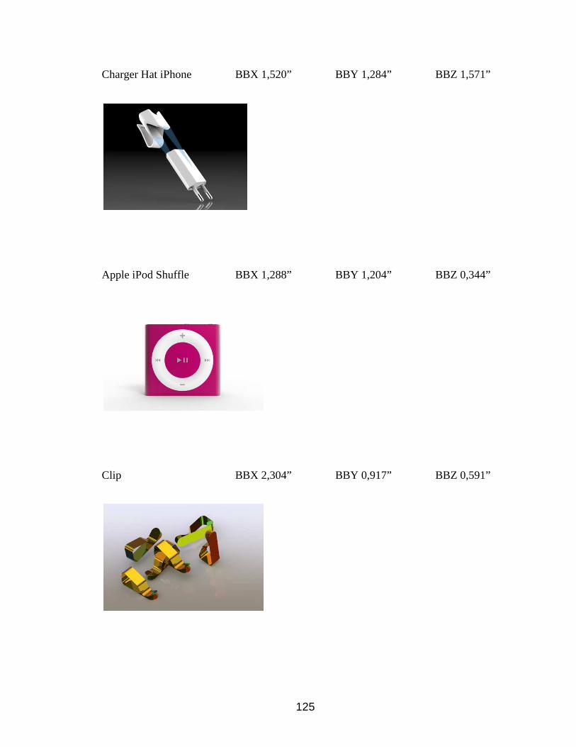
125
Charger Hat iPhone BBX 1,520” BBY 1,284” BBZ 1,571”
Apple iPod Shuffle BBX 1,288” BBY 1,204” BBZ 0,344”
Clip BBX 2,304” BBY 0,917” BBZ 0,591”

EOS UK Plug Fixer
JBL Speaker
Inline Acustic Box
126
BBX 1,580” BBY 0,946”
BBX 2,854“ BBY 2,253“
BBX 11,304“ BBY 16,501“
BBZ 1,512”
BBZ 2,750“
BBZ 10,589“

127
Piston Sample BBX 1,625“ BBY 2,443“ BBZ 1,575“
Cat Pumpkin BBX 11,828“ BBY 11,311“ BBZ 11,423“
Logo Vietnam Electricity BBX 8,549“ BBY 1,547“ BBZ 8,268“

128
2 Euro BBX 1,018“ BBY 1,018“ BBZ 0,095“
Chocolate Riddle BBX 2,280“ BBY 0,305“ BBZ 5,197“
Battery Bracket BBX 2,524“ BBY 0,407“ BBZ 0,850“

129
Laptop Paper Holder BBX 4,071“ BBY 2,023“ BBZ 0,606“
3M Stethoscope BBX 11,322“ BBY 0,979“ BBZ 6,558“
Traffic Light BBX 2,496“ BBY 6,106“ BBZ 2,361“

130
iPhone 5C BBX 2,430“ BBY 5.089“ BBZ 0,353“
iPhone 4S Irig Case BBX 3,816“ BBY 4,858“ BBZ 1,133“
Apple Lightning Pin
Adapters BBX 1,068“ BBY 1,080“ BBZ 0,222“

131
Ribbon Stands BBX 4,249“ BBY 2,267“ BBZ 2,867“
iShare BBX 4,168“ BBY 1,018“ BBZ 0,551“
iPhone 5 Cover BBX 2,791“ BBY 5,122“ BBZ 0,866“

132
iPod BBX 2,516“ BBY 4,229“ BBZ 0,551“
Apple of Eden Lamp BBX 6,716“ BBY 6,681“ BBZ 6,495“
Apple WiFi Router BBX 14,248“ BBY 5,498“ BBZ 6,339“

133
iPad Model BBX 1,832“ BBY 0,130“ BBZ 2,196“
Speaker BBX 4,485“ BBY 8,386“ BBZ 4,500“
Playing Card BBX 2,585“ BBY 3,619“ BBZ 0,030“

134
Shaft Lubricator BBX 6,651“ BBY 4,966“ BBZ 6,929“
Coupling Flange BBX 1,221“ BBY 13,637“ BBZ 13,189“
Clock BBX 6,106“ BBY 9,917“ BBZ 2,626“

135
Edge Protector BBX 1,622“ BBY 1,637“ BBZ 1,575“
Soft Jaws – Full Wrap BBX 12,211“ BBY 1,710“ BBZ 11,811“
Rubber Stamp BBX 4,067“ BBY 6,214“ BBZ 3,937“

USB Keychain Holder
Junction Box
Engine Crankcase Covers
136
BBX 0,691“ BBY 0,329“
BBX 3,420“ BBY 2,353“
Engine Crankcase Covers BBX 2,972“ BBY 15,669“
BBZ 0,938“
BBZ 5,039“
BBZ 7,126“

137
Shaft and Guide Support BBX 4,437“ BBY 5,618“ BBZ 2,008“
Mount for Maxon
Gearmotor BBX 1,506“ BBY 1,370“ BBZ 1,102“
Face Mill BBX 8,544“ BBY 8,537“ BBZ 2,223“

138
EMI Filter BBX 2,378“ BBY 2,497“ BBZ 1,900“
Sony PCM D50 BBX 3,318“ BBY 6,277“ BBZ 1,343“
FPV Camera Turnigy 600 BBX 1,301“ BBY 1,233“ BBZ 1,159“

139
Grill for Stove BBX 16,283“ BBY 8,142“ BBZ 0,472“
Engine Spoket BBX 3,852“ BBY 3,834“ BBZ 0,394“
Sheet Metal Pipe BBX 3,053“ BBY 3.053“ BBZ 11,811“

140
Electric Eel Eurosocket BBX 12,886“ BBY 1,851“ BBZ 1,459“
Ship’s Propeller BBX 9,189“ BBY 2,768“ BBZ 8,887“
Can Cover BBX 2,401“ BBY 0,326“ BBZ 2,322“

141
Mount for IG BBX 1,750“ BBY 2,361“ BBZ 3,094“
Record Player Clip BBX 0,749“ BBY 1,070“ BBZ 1,892“
Engine Mounts BBX 6,885“ BBY 2,544“ BBZ 4,075“

142
Jet Engine Bracket BBX 7,505“ BBY 2,646“ BBZ 3,963“
Battery Cover BBX 2,227“ BBY 0,183“ BBZ 1,177“
Roller Handle and Knob BBX 5,745“ BBY 1,990“ BBZ 1,535“

143
Pasta Spoon BBX 2,897“ BBY 2,269“ BBZ 11,071“
Pivot Guide BBX 7,309“ BBY 4,375“ BBZ 3,543“
Rotate Drill for the Dentist BBX 5,638” BBY 0,407” BBZ 2,087”

144
Sheet Metal Part Box BBX 5,266” BBY 1,323” BBZ 3,911”
Thermoform Tray BBX 9,977” BBY 1,750” BBZ 6,893”
Fixture Medical Devices BBX 1,723” BBY 0,933” BBZ 0,125”

145
Electrical Box BBX 8,796” BBY 1,876” BBZ 6,025”
Medicine Spoon BBX 10,205” BBY 0,724” BBZ 3,739”
Walking Stick Handle BBX 9,037” BBY 3,769” BBZ 1,445”

146
Toothbrush BBX 7,333” BBY 0,730” BBZ 0,672”
Tooth BBX 2,421” BBY 4,366” BBZ 1,267”
Plastic Vending Cup BBX 7,337” BBY 8,065” BBZ 7,100”

147
Inhaler Case BBX 0,552” BBY 1,397” BBZ 1,151”
Impression Tray BBX 2,384” BBY 0,766” BBZ 2,886”
(http://www.gceurope.com/products/op_impression_taking.php)
The Solid Works Model for the Impression Tray was done by Joe Vicar, Laser
Development Engineer from the University of Louisville.
Carotid Bifurcation BBX 0,002” BBY 0,001” BBZ 0,006”

148
Pill Box BBX 3,541” BBY 0,979” BBZ 3,425”
Digital Timer BBX 2,456” BBY 2,428” BBZ 0,563”
Ferrule, Clamp Tool BBX 2,051” BBY 2,051” BBZ 1,750”
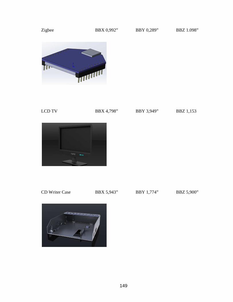
149
Zigbee BBX 0,992” BBY 0,289” BBZ 1.098”
LCD TV BBX 4,798” BBY 3,949” BBZ 1,153
CD Writer Case BBX 5,943” BBY 1,774” BBZ 5,900”

Roof Hook
Portable Stove
DVD Burner
150
BBX 3,827” BBY 5,659”
BBX 8,541” BBY 1,692”
BBX 6,961” BBY 1,677”
BBZ 5,669”
BBZ 7,625”
BBZ 5,756”
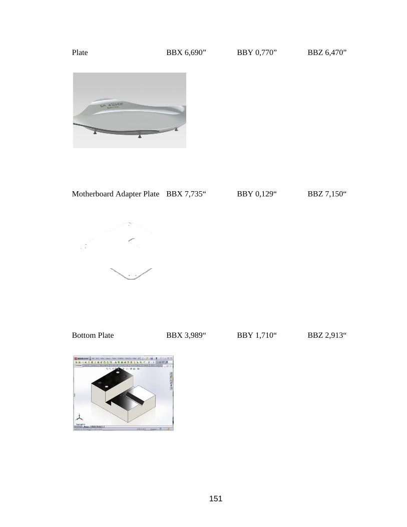
Plate
Motherboard Adapter Plate
Bottom Plate
151
BBX 6,690” BBY 0,770”
Motherboard Adapter Plate BBX 7,735“ BBY 0,129“
BBX 3,989“ BBY 1,710“
BBZ 6,470”
BBZ 7,150“
BBZ 2,913“

152
Faceplate Spider BBX 8,937“ BBY 5,377“ BBZ 0,032“
Carbon Fiber Dash BBX 15,155“ BBY 5,625“ BBZ 2,250“
Excluded the mouth tray all photos and models were adapted from grabcad.com.

153
APPENDIX B: MATLAB GA for Bin Packing
ga_2d_box_packing.m
% main box sizes:
a=2;
b=1;
Nb=30; % number of boxes
% random boxes sizes:
mab=mean([a b]);
aa=0.05*mab+0.3*mab*rand(1,Nb);
bb=0.05*mab+0.3*mab*rand(1,Nb);
m2=min([aa bb]/2); % smallest half-size
AA=aa.*bb; % boxes areas

154
penalty=0.2*a*b;
nac=0.8; % negative area coefficient
N=500; % population size
ng=5000; % number of generations
pmpe=0.05; % places exchange mutation probability
pmbj=0.01; % big gauss jump
pmsj=0.02; % small gauss jump
pmrr=0.05; % random rotation
pmvi=0.05; % random visible/invisible
pmne=0.1; % move to nearest adge
figure;
%ha1=axes;
ha1=subplot(2,1,1);
plot([0 a a 0 0], [0 0 b b 0],'b-');
xlim([-0.1*a 1.1*a]);
ylim([-0.1*b 1.1*b]);

155
set(ha1,'NextPlot','add');
ht=title(ha1,'start');
ha2=subplot(2,1,2);
drawnow;
set_cl; % set color table cl to plot boxes with different colors
% random initial population:
G=zeros(N,4*Nb);
Gch=zeros(N,4*Nb); % children
for Nc=1:N % for each individual
G1=zeros(4,Nb); % one individual
% G1(1,i)=1 if i-box is visible
% G1(2,i)=1 if i-box is rotated at 90 degrees
% G1(3,i) - x-coordinate of i-box center
% G1(4,i) - y-coordinate of i-box center
G1(1,:)=double(rand(1,Nb)<0.2);

156
G1(2,:)=double(rand(1,Nb)<0.5);
G1(3,:)=m2+(a-m2)*rand(1,Nb);
G1(4,:)=m2+(b-m2)*rand(1,Nb);
G(Nc,:)=(G1(:))'; % (G1(:))' converts matrix to row-vector
end
hi=imagesc(G,'parent',ha2);
drawnow;
Gpr1=zeros(4,Nb);
Gpr2=zeros(4,Nb); % two parents
Gch1=zeros(4,Nb);
Gch2=zeros(4,Nb); % two children
for ngc=1:ng % generations counting
% find fitnesses:
fitnesses=zeros(N,1);
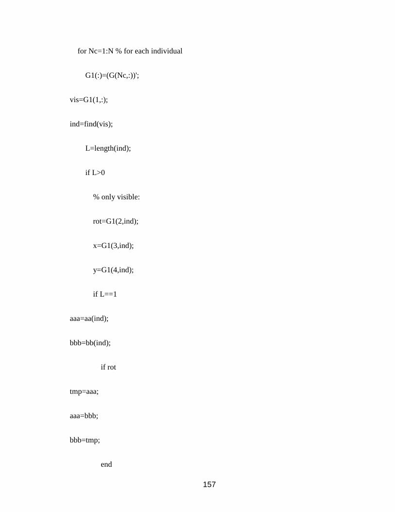
157
for Nc=1:N % for each individual
G1(:)=(G(Nc,:))';
vis=G1(1,:);
ind=find(vis);
L=length(ind);
if L>0
% only visible:
rot=G1(2,ind);
x=G1(3,ind);
y=G1(4,ind);
if L==1
aaa=aa(ind);
bbb=bb(ind);
if rot
tmp=aaa;
aaa=bbb;
bbb=tmp;
end

158
A0=AA(ind); % box area
x1=max([x-aaa/2 0]);
y1=max([y-bbb/2 0]);
x2=min([x+aaa/2 a]);
y2=min([y+bbb/2 b]);
% x1 - x2, y1 - y2 is box (part of current box) that inside main box
if (x1>=x2)||(y1>=y2)
A=0; % box that inside main box area
else
A=(x2-x1)*(y2-y1); % box that inside main box area
end
%if A<A0 % if not fully inside main box
if (aaa/2<=x)&&(x<=a-aaa/2)&&(bbb/2<=y)&&(y<=b-bbb/2) % if filly inside
fitness=A;
else
fitness=A-nac*(A0-A)-penalty;
end
else

159
fitness=0;
ispen=false; % true if penality
% check cross with main box:
% add boxes arreas and strong subtract out areas:
for n=1:L % for each box
ind1=ind(n);
aaa=aa(ind1);
bbb=bb(ind1);
if rot(n)
tmp=aaa;
aaa=bbb;
bbb=tmp;
end
A0=AA(ind1); % box area
x1=max([x(n)-aaa/2 0]);
y1=max([y(n)-bbb/2 0]);
x2=min([x(n)+aaa/2 a]);

160
y2=min([y(n)+bbb/2 b]);
% x1 - x2, y1 - y2 is box (part of current box) that inside main box
if (x1>=x2)||(y1>=y2)
A=0; % box that inside main box area
else
A=(x2-x1)*(y2-y1); % box that inside main box area
end
%if A<A0 % if not fully inside main box
%fitness=fitness + A-nac*(A0-A);
%ispen=true; % penality
%else
%fitness=fitness + A;
%end
if (aaa/2<=x(n))&&(x(n)<=a-aaa/2)&&(bbb/2<=y(n))&&(y(n)<=b-bbb/2) %
if filly inside
fitness=fitness + A;
else

161
fitness=fitness + A-nac*(A0-A);
ispen=true; % penality
end
end
% for each pair of boxes:
for n1=1:L-1
ind1=ind(n1);
aaa1=aa(ind1);
bbb1=bb(ind1);
if rot(n1)
tmp=aaa1;
aaa1=bbb1;
bbb1=tmp;
end
A1=AA(ind1);
x1=x(n1);

162
y1=y(n1); % position of 1st box of pair
for n2=n1+1:L
ind2=ind(n2);
aaa2=aa(ind2);
bbb2=bb(ind2);
if rot(n2)
tmp=aaa2;
aaa2=bbb2;
bbb2=tmp;
end
A2=AA(ind2);
x2=x(n2);
y2=y(n2); % position of 2nd box of pair
dx=abs(x1-x2);
dy=abs(y1-y2); % distancies
a12=(aaa1/2+aaa2/2);
b12=(bbb1/2+bbb2/2);
if (dx<a12)&&(dy<b12) % if cross

163
ispen=true;
Ac=(a12-dx)*(b12-dy); % area of cross
fitness=fitness-Ac-Ac; % becuse area of n1 and n2 was added fully
fitness=fitness-2*nac*Ac;
end
end
end
if ispen
fitness=fitness-penalty;
end
end
else
fitness=0;
end
fitnesses(Nc)=fitness;

164
end
[fb bi]=max(fitnesses); % best
% plot best:
G1(:)=(G(bi,:))';
Gb=G(bi,:); % best
if mod(ngc,10)==0
cla(ha1);
Atmp=0;
for Nbc=1:Nb
vis1=G1(1,Nbc);
if vis1
rot1=G1(2,Nbc);
aaa=aa(Nbc);
bbb=bb(Nbc);
if rot1
tmp=aaa;

165
aaa=bbb;
bbb=tmp;
end
x=G1(3,Nbc);
y=G1(4,Nbc);
plot([x-aaa/2 x+aaa/2 x+aaa/2 x-aaa/2 x-aaa/2],...
[y-bbb/2 y-bbb/2 y+bbb/2 y+bbb/2 y-bbb/2],...
'-','color',cl(Nbc,:),...
'parent',ha1);
hold on;
Atmp=Atmp+aaa*bbb;
end
end
plot([0 a a 0 0], [0 0 b b 0],'b-','parent',ha1);
xlim(ha1,[-0.1*a 1.1*a]);
ylim(ha1,[-0.1*b 1.1*b]);
set(hi,'Cdata',G);

166
nvb=length(find(G1(1,:))); % number of visible boxes
set(ht,'string',[' generation: ' num2str(ngc) ', boxes: ' num2str(nvb) ', area: '
num2str(fb)]);
drawnow;
end
% prepare for crossover, selection:
fmn=min(fitnesses);
fst=std(fitnesses);
if fst<1e-7
fst=1e-7;
end
fmn1=fmn-0.01*fst; % little low then minimum
P=fitnesses-fmn1; % positive values
p=P/sum(P); % probabilities

167
ii=roulette_wheel_indexes(N,p);
Gp=G(ii,:); % parents
% crossover:
for n=1:2:N
pr1=Gp(n,:);
pr2=Gp(n+1,:); % two parents
% in matrix form:
Gpr1(:)=pr1';
Gpr2(:)=pr2';
for Nbc=1:Nb
% visibility:
if rand<0.5
Gch1(1,Nbc)=Gpr1(1,Nbc);
else
Gch1(1,Nbc)=Gpr2(1,Nbc);

168
end
if rand<0.5
Gch2(1,Nbc)=Gpr1(1,Nbc);
else
Gch2(1,Nbc)=Gpr2(1,Nbc);
end
% rotation:
if rand<0.5
Gch1(2,Nbc)=Gpr1(2,Nbc);
else
Gch1(2,Nbc)=Gpr2(2,Nbc);
end
if rand<0.5
Gch2(2,Nbc)=Gpr1(2,Nbc);
else
Gch2(2,Nbc)=Gpr2(2,Nbc);
end

169
% position:
% child 1:
%i3=ceil(3*rand);
%i3=roulette_wheel_indexes(1,[0.2 0.4 0.4]);
i3=1+ceil(2*rand);
switch i3
case 1 % get mean position
Gch1(3,Nbc)=(Gpr1(3,Nbc)+Gpr2(3,Nbc))/2;
Gch1(4,Nbc)=(Gpr1(4,Nbc)+Gpr2(4,Nbc))/2;
case 2 %get position of parent 1
Gch1(3,Nbc)=Gpr1(3,Nbc);
Gch1(4,Nbc)=Gpr1(4,Nbc);
case 3 %get position of parent 2
Gch1(3,Nbc)=Gpr2(3,Nbc);
Gch1(4,Nbc)=Gpr2(4,Nbc);
end
% child 2:

170
%i3=ceil(3*rand);
%i3=roulette_wheel_indexes(1,[0.2 0.4 0.4]);
i3=1+ceil(2*rand);
switch i3
case 1 % get mean position
Gch2(3,Nbc)=(Gpr1(3,Nbc)+Gpr2(3,Nbc))/2;
Gch2(4,Nbc)=(Gpr1(4,Nbc)+Gpr2(4,Nbc))/2;
case 2 %get position of parent 1
Gch2(3,Nbc)=Gpr1(3,Nbc);
Gch2(4,Nbc)=Gpr1(4,Nbc);
case 3 %get position of parent 2
Gch2(3,Nbc)=Gpr2(3,Nbc);
Gch2(4,Nbc)=Gpr2(4,Nbc);
end
end
ch1=(Gch1(:))';
ch2=(Gch2(:))';

171
Gch(n,:)=ch1;
Gch(n+1,:)=ch2;
end
G=Gch; % now children
% mutations:
% places exchange
for Nc=1:N % for each individual
if rand<pmpe
G1(:)=(G(Nc,:))';
ir1=ceil(Nb*rand);
ir2=ceil(Nb*rand);
tmp1=G1(3:4,ir1);
G1(3:4,ir1)=G1(3:4,ir2);
G1(3:4,ir2)=tmp1;
G(Nc,:)=(G1(:))';
end

172
end
% big gauss jump:
for Nc=1:N % for each individual
if rand<pmbj
G1(:)=(G(Nc,:))';
ir=ceil(Nb*rand);
G1(3:4,ir)=G1(3:4,ir)+[0.05*a*randn;
0.05*b*randn];
G(Nc,:)=(G1(:))';
end
end
% small gauss jump:
for Nc=1:N % for each individual
if rand<pmsj
G1(:)=(G(Nc,:))';
ir=ceil(Nb*rand);

173
G1(3:4,ir)=G1(3:4,ir)+[0.005*a*randn;
0.005*b*randn];
G(Nc,:)=(G1(:))';
end
end
% random rotation:
for Nc=1:N % for each individual
if rand<pmrr
G1(:)=(G(Nc,:))';
ir=ceil(Nb*rand);
G1(2,ir)=double(rand<0.5);
G(Nc,:)=(G1(:))';
end
end
% random visible/invisible:
for Nc=1:N % for each individual
if rand<pmvi
G1(:)=(G(Nc,:))';

174
ir=ceil(Nb*rand);
G1(1,ir)=double(rand<0.5);
G(Nc,:)=(G1(:))';
end
end
% move to nearest edge:
for Nc=1:N % for each individual
if rand<pmne
G1(:)=(G(Nc,:))';
ir=ceil(Nb*rand); % random small box
rv=find((G1(1,:))&((1:Nb)~=Nc)); % find rest visible
if rand<0.5
% to veritcile edge
eax=[G1(3,rv)-aa(rv)/2 G1(3,rv)+aa(rv)/2 0 a]; % edge xs
deax=[(G1(3,ir)-aa(ir)/2) - eax (G1(3,ir)+aa(ir)/2) - eax]; % distancies
[dmnindm]=min(abs(deax));
G1(3,ir)=G1(3,ir)-deax(indm);
else

175
% to horizontal edge
eay=[G1(4,rv)-bb(rv)/2 G1(4,rv)+bb(rv)/2 0 b]; % edge ys
deay=[(G1(4,ir)-bb(ir)/2) - eay (G1(4,ir)+bb(ir)/2) - eay]; % distancies
[dmnindm]=min(abs(deay));
G1(4,ir)=G1(4,ir)-deay(indm);
end
end
end
% ellitism:
G(1,:)=Gb;
end
http://www.mathworks.com/matlabcentral/fileexchange/index?utf8=%E2%9C%93&term
=ga_2d_box_packing.m+category%3A%22Mathematics%22+type%3A%22script%22+t
ype%3A%22Function%22

176
APPENDIX C: LINGO model and solution
Lingo model to meet the limitation of the Build volume: sets: indexj /1..120/: V, S, d, X; endsets Data: !attribute values; V = 0.11236192 0.04648375 0.00114308 0.01814988 4.7396E-05 0.09326288 0.04223786 0.26715312 3.11935891 1.08392876 0.0407376 0.0149604 0.00270599 4.0698E-05 1.2505E-05 0.00050692 4.4616E-05 0.00001408 0.00016606 0.00323417 5.1084E-05 0.00003128 0.40954728 1.63721859 0.03132464 0.32616288 0.012514 0.25455917 0.35193453

177
0.76125862 0.06685119 0.01967764 0.04581432 0.0689472 0.0686394 0.32616288 42.9375274 760.807465 352.309706 694.256744 114.004464 3.06608928 0.53345869 1.24864589 2.25995616 17.6826705 1975.13762 6.25255313 1528.24328 109.346805 0.09845078 3.6139938 0.8731778 4.9907936 72.6904328 35.9829999 4.36529331 21.003699 0.25606368 27.6163288 2.33790622 12.3799047 5.86273036 291.428026 496.56876 0.52299936 169.250445 0.28065345 228.857013 219.607098 159.012708 4.18196205 246.623247 99.4971947 0.21324398 40.5501431 331.845478

178
50.0535485 2.27366844 162.145905 11.2819454 27.9707765 1.85919015 62.5759598 5.81881579 110.088075 34.8000476 226.042196 45.6393574 1.81748977 12.7836345 1.51630556 71.375418 78.6981655 0.47967576 17.5489643 72.7729268 113.294068 5.27025158 1.2E-08 0.88758674 11.8732386 0.20094488 49.2173546 3.35726358 120.350057 4.78896794 3.59727648 7.36155175 27.2476163 13.392299 99.4203084 420.127626 27.6253024 0.31478342 21.8462392 62.2030038 122.773493 110.191712 67.1932243 ; S = 11.236192 4.6483752 0.114308

179
1.814988 0.0047396 9.3262884 4.2237864 26.715312 311.935891 108.392876 4.07376 1.49604 0.2705992 0.0040698 0.0012505 0.050692 0.0044616 0.001408 0.0166056 0.3234168 0.0051084 0.003128 40.954728 163.721859 3.132464 32.6162881 1.2513999 25.4559172 35.1934528 76.1258616 6.685119 1.9677636 4.581432 6.89472 6.86394 32.6162881 4293.75274 76080.7465 35230.9706 69425.6744 11400.4464 306.608928 53.3458688 124.864589 225.995616 1768.26705 197513.762 625.255313 152824.328 10934.6805 9.845078

180
361.39938 87.31778 499.07936 7269.04328 3598.29999 436.529331 2100.3699 25.606368 2761.63288 233.790622 1237.99047 586.273036 29142.8026 49656.876 52.299936 16925.0445 28.065345 22885.7013 21960.7098 15901.2708 418.196205 24662.3247 9949.71947 21.3243982 4055.01431 33184.5478 5005.35485 227.366844 16214.5905 1128.19454 2797.07765 185.919015 6257.59598 581.881579 11008.8075 3480.00476 22604.2196 4563.93574 181.748977 1278.36345 151.630556 7137.5418 7869.81655 47.9675757 1754.89643 7277.29268 11329.4068 527.025158

181
0.0000012 88.7586744 1187.32386 20.0944875 4921.73546 335.726358 12035.0057 478.896794 359.727648 736.155175 2724.76163 1339.2299 9942.03084 42012.7626 2762.53024 31.4783424 2184.62392 6220.30038 12277.3493 11019.1712 6719.32243 ; d = 8 9 11 4 10 7 11 4 4 5 5 3 7 7 9 6 5 7 12 6 3 10 5 5 6

182
8 6 4 5 10 9 10 7 11 10 12 3 5 8 11 5 7 6 4 12 4 9 8 10 5 6 9 7 6 10 8 11 9 10 7 4 5 6 6 12 8 9 4 9 11 4 6 4

183
7 9 11 3 12 9 12 8 12 8 10 12 5 9 5 11 3 8 8 3 10 3 5 11 4 11 3 9 8 4 8 7 12 8 7 8 7 9 5 6 7 11 4 6 9 11 5 ;

184
Enddata Max = @Sum(indexj(j): S(j)*X(j)); @SUM(indexj(j):V(j)*X(j))<=3510; @FOR(indexj(j): @GIN(x(j))); Lingo Solution Report:
Global optimal solution found. Objective value: 351000.3 Objective bound: 351000.3 Infeasibilities: 0.000000 Extended solver steps: 0 Total solver iterations: 11 Variable Value Reduced Cost V( 1) 0.1123619 0.000000 V( 2) 0.4648375E-01 0.000000 V( 3) 0.1143080E-02 0.000000 V( 4) 0.1814988E-01 0.000000 V( 5) 0.4739600E-04 0.000000

185
V( 6) 0.9326288E-01 0.000000 V( 7) 0.4223786E-01 0.000000 V( 8) 0.2671531 0.000000 V( 9) 3.119359 0.000000 V( 10) 1.083929 0.000000 V( 11) 0.4073760E-01 0.000000 V( 12) 0.1496040E-01 0.000000 V( 13) 0.2705990E-02 0.000000 V( 14) 0.4069800E-04 0.000000 V( 15) 0.1250500E-04 0.000000 V( 16) 0.5069200E-03 0.000000 V( 17) 0.4461600E-04 0.000000 V( 18) 0.1408000E-04 0.000000 V( 19) 0.1660600E-03 0.000000 V( 20) 0.3234170E-02 0.000000 V( 21) 0.5108400E-04 0.000000 V( 22) 0.3128000E-04 0.000000 V( 23) 0.4095473 0.000000 V( 24) 1.637219 0.000000 V( 25) 0.3132464E-01 0.000000 V( 26) 0.3261629 0.000000 V( 27) 0.1251400E-01 0.000000 V( 28) 0.2545592 0.000000 V( 29) 0.3519345 0.000000 V( 30) 0.7612586 0.000000 V( 31) 0.6685119E-01 0.000000 V( 32) 0.1967764E-01 0.000000 V( 33) 0.4581432E-01 0.000000 V( 34) 0.6894720E-01 0.000000 V( 35) 0.6863940E-01 0.000000 V( 36) 0.3261629 0.000000 V( 37) 42.93753 0.000000 V( 38) 760.8075 0.000000 V( 39) 352.3097 0.000000 V( 40) 694.2567 0.000000 V( 41) 114.0045 0.000000 V( 42) 3.066089 0.000000 V( 43) 0.5334587 0.000000 V( 44) 1.248646 0.000000 V( 45) 2.259956 0.000000 V( 46) 17.68267 0.000000 V( 47) 1975.138 0.000000 V( 48) 6.252553 0.000000 V( 49) 1528.243 0.000000 V( 50) 109.3468 0.000000 V( 51) 0.9845078E-01 0.000000 V( 52) 3.613994 0.000000 V( 53) 0.8731778 0.000000

186
V( 54) 4.990794 0.000000 V( 55) 72.69043 0.000000 V( 56) 35.98300 0.000000 V( 57) 4.365293 0.000000 V( 58) 21.00370 0.000000 V( 59) 0.2560637 0.000000 V( 60) 27.61633 0.000000 V( 61) 2.337906 0.000000 V( 62) 12.37990 0.000000 V( 63) 5.862730 0.000000 V( 64) 291.4280 0.000000 V( 65) 496.5688 0.000000 V( 66) 0.5229994 0.000000 V( 67) 169.2504 0.000000 V( 68) 0.2806535 0.000000 V( 69) 228.8570 0.000000 V( 70) 219.6071 0.000000 V( 71) 159.0127 0.000000 V( 72) 4.181962 0.000000 V( 73) 246.6232 0.000000 V( 74) 99.49719 0.000000 V( 75) 0.2132440 0.000000 V( 76) 40.55014 0.000000 V( 77) 331.8455 0.000000 V( 78) 50.05355 0.000000 V( 79) 2.273668 0.000000 V( 80) 162.1459 0.000000 V( 81) 11.28195 0.000000 V( 82) 27.97078 0.000000 V( 83) 1.859190 0.000000 V( 84) 62.57596 0.000000 V( 85) 5.818816 0.000000 V( 86) 110.0881 0.000000 V( 87) 34.80005 0.000000 V( 88) 226.0422 0.000000 V( 89) 45.63936 0.000000 V( 90) 1.817490 0.000000 V( 91) 12.78363 0.000000 V( 92) 1.516306 0.000000 V( 93) 71.37542 0.000000 V( 94) 78.69817 0.000000 V( 95) 0.4796758 0.000000 V( 96) 17.54896 0.000000 V( 97) 72.77293 0.000000 V( 98) 113.2941 0.000000 V( 99) 5.270252 0.000000 V( 100) 0.1200000E-07 0.000000 V( 101) 0.8875867 0.000000

187
V( 102) 11.87324 0.000000 V( 103) 0.2009449 0.000000 V( 104) 49.21735 0.000000 V( 105) 3.357264 0.000000 V( 106) 120.3501 0.000000 V( 107) 4.788968 0.000000 V( 108) 3.597276 0.000000 V( 109) 7.361552 0.000000 V( 110) 27.24762 0.000000 V( 111) 13.39230 0.000000 V( 112) 99.42031 0.000000 V( 113) 420.1276 0.000000 V( 114) 27.62530 0.000000 V( 115) 0.3147834 0.000000 V( 116) 21.84624 0.000000 V( 117) 62.20300 0.000000 V( 118) 122.7735 0.000000 V( 119) 110.1917 0.000000 V( 120) 67.19322 0.000000 S( 1) 11.23619 0.000000 S( 2) 4.648375 0.000000 S( 3) 0.1143080 0.000000 S( 4) 1.814988 0.000000 S( 5) 0.4739600E-02 0.000000 S( 6) 9.326288 0.000000 S( 7) 4.223786 0.000000 S( 8) 26.71531 0.000000 S( 9) 311.9359 0.000000 S( 10) 108.3929 0.000000 S( 11) 4.073760 0.000000 S( 12) 1.496040 0.000000 S( 13) 0.2705992 0.000000 S( 14) 0.4069800E-02 0.000000 S( 15) 0.1250500E-02 0.000000 S( 16) 0.5069200E-01 0.000000 S( 17) 0.4461600E-02 0.000000 S( 18) 0.1408000E-02 0.000000 S( 19) 0.1660560E-01 0.000000 S( 20) 0.3234168 0.000000 S( 21) 0.5108400E-02 0.000000 S( 22) 0.3128000E-02 0.000000 S( 23) 40.95473 0.000000 S( 24) 163.7219 0.000000 S( 25) 3.132464 0.000000 S( 26) 32.61629 0.000000 S( 27) 1.251400 0.000000 S( 28) 25.45592 0.000000 S( 29) 35.19345 0.000000

188
S( 30) 76.12586 0.000000 S( 31) 6.685119 0.000000 S( 32) 1.967764 0.000000 S( 33) 4.581432 0.000000 S( 34) 6.894720 0.000000 S( 35) 6.863940 0.000000 S( 36) 32.61629 0.000000 S( 37) 4293.753 0.000000 S( 38) 76080.75 0.000000 S( 39) 35230.97 0.000000 S( 40) 69425.67 0.000000 S( 41) 11400.45 0.000000 S( 42) 306.6089 0.000000 S( 43) 53.34587 0.000000 S( 44) 124.8646 0.000000 S( 45) 225.9956 0.000000 S( 46) 1768.267 0.000000 S( 47) 197513.8 0.000000 S( 48) 625.2553 0.000000 S( 49) 152824.3 0.000000 S( 50) 10934.68 0.000000 S( 51) 9.845078 0.000000 S( 52) 361.3994 0.000000 S( 53) 87.31778 0.000000 S( 54) 499.0794 0.000000 S( 55) 7269.043 0.000000 S( 56) 3598.300 0.000000 S( 57) 436.5293 0.000000 S( 58) 2100.370 0.000000 S( 59) 25.60637 0.000000 S( 60) 2761.633 0.000000 S( 61) 233.7906 0.000000 S( 62) 1237.990 0.000000 S( 63) 586.2730 0.000000 S( 64) 29142.80 0.000000 S( 65) 49656.88 0.000000 S( 66) 52.29994 0.000000 S( 67) 16925.04 0.000000 S( 68) 28.06535 0.000000 S( 69) 22885.70 0.000000 S( 70) 21960.71 0.000000 S( 71) 15901.27 0.000000 S( 72) 418.1962 0.000000 S( 73) 24662.32 0.000000 S( 74) 9949.719 0.000000 S( 75) 21.32440 0.000000 S( 76) 4055.014 0.000000 S( 77) 33184.55 0.000000

189
S( 78) 5005.355 0.000000 S( 79) 227.3668 0.000000 S( 80) 16214.59 0.000000 S( 81) 1128.195 0.000000 S( 82) 2797.078 0.000000 S( 83) 185.9190 0.000000 S( 84) 6257.596 0.000000 S( 85) 581.8816 0.000000 S( 86) 11008.81 0.000000 S( 87) 3480.005 0.000000 S( 88) 22604.22 0.000000 S( 89) 4563.936 0.000000 S( 90) 181.7490 0.000000 S( 91) 1278.363 0.000000 S( 92) 151.6306 0.000000 S( 93) 7137.542 0.000000 S( 94) 7869.817 0.000000 S( 95) 47.96758 0.000000 S( 96) 1754.896 0.000000 S( 97) 7277.293 0.000000 S( 98) 11329.41 0.000000 S( 99) 527.0252 0.000000 S( 100) 0.1200000E-05 0.000000 S( 101) 88.75867 0.000000 S( 102) 1187.324 0.000000 S( 103) 20.09449 0.000000 S( 104) 4921.735 0.000000 S( 105) 335.7264 0.000000 S( 106) 12035.01 0.000000 S( 107) 478.8968 0.000000 S( 108) 359.7276 0.000000 S( 109) 736.1552 0.000000 S( 110) 2724.762 0.000000 S( 111) 1339.230 0.000000 S( 112) 9942.031 0.000000 S( 113) 42012.76 0.000000 S( 114) 2762.530 0.000000 S( 115) 31.47834 0.000000 S( 116) 2184.624 0.000000 S( 117) 6220.300 0.000000 S( 118) 12277.35 0.000000 S( 119) 11019.17 0.000000 S( 120) 6719.322 0.000000 D( 1) 8.000000 0.000000 D( 2) 9.000000 0.000000 D( 3) 11.00000 0.000000 D( 4) 4.000000 0.000000 D( 5) 10.00000 0.000000

190
D( 6) 7.000000 0.000000 D( 7) 11.00000 0.000000 D( 8) 4.000000 0.000000 D( 9) 4.000000 0.000000 D( 10) 5.000000 0.000000 D( 11) 5.000000 0.000000 D( 12) 3.000000 0.000000 D( 13) 7.000000 0.000000 D( 14) 7.000000 0.000000 D( 15) 9.000000 0.000000 D( 16) 6.000000 0.000000 D( 17) 5.000000 0.000000 D( 18) 7.000000 0.000000 D( 19) 12.00000 0.000000 D( 20) 6.000000 0.000000 D( 21) 3.000000 0.000000 D( 22) 10.00000 0.000000 D( 23) 5.000000 0.000000 D( 24) 5.000000 0.000000 D( 25) 6.000000 0.000000 D( 26) 8.000000 0.000000 D( 27) 6.000000 0.000000 D( 28) 4.000000 0.000000 D( 29) 5.000000 0.000000 D( 30) 10.00000 0.000000 D( 31) 9.000000 0.000000 D( 32) 10.00000 0.000000 D( 33) 7.000000 0.000000 D( 34) 11.00000 0.000000 D( 35) 10.00000 0.000000 D( 36) 12.00000 0.000000 D( 37) 3.000000 0.000000 D( 38) 5.000000 0.000000 D( 39) 8.000000 0.000000 D( 40) 11.00000 0.000000 D( 41) 5.000000 0.000000 D( 42) 7.000000 0.000000 D( 43) 6.000000 0.000000 D( 44) 4.000000 0.000000 D( 45) 12.00000 0.000000 D( 46) 4.000000 0.000000 D( 47) 9.000000 0.000000 D( 48) 8.000000 0.000000 D( 49) 10.00000 0.000000 D( 50) 5.000000 0.000000 D( 51) 6.000000 0.000000 D( 52) 9.000000 0.000000 D( 53) 7.000000 0.000000

191
D( 54) 6.000000 0.000000 D( 55) 10.00000 0.000000 D( 56) 8.000000 0.000000 D( 57) 11.00000 0.000000 D( 58) 9.000000 0.000000 D( 59) 10.00000 0.000000 D( 60) 7.000000 0.000000 D( 61) 4.000000 0.000000 D( 62) 5.000000 0.000000 D( 63) 6.000000 0.000000 D( 64) 6.000000 0.000000 D( 65) 12.00000 0.000000 D( 66) 8.000000 0.000000 D( 67) 9.000000 0.000000 D( 68) 4.000000 0.000000 D( 69) 9.000000 0.000000 D( 70) 11.00000 0.000000 D( 71) 4.000000 0.000000 D( 72) 6.000000 0.000000 D( 73) 4.000000 0.000000 D( 74) 7.000000 0.000000 D( 75) 9.000000 0.000000 D( 76) 11.00000 0.000000 D( 77) 3.000000 0.000000 D( 78) 12.00000 0.000000 D( 79) 9.000000 0.000000 D( 80) 12.00000 0.000000 D( 81) 8.000000 0.000000 D( 82) 12.00000 0.000000 D( 83) 8.000000 0.000000 D( 84) 10.00000 0.000000 D( 85) 12.00000 0.000000 D( 86) 5.000000 0.000000 D( 87) 9.000000 0.000000 D( 88) 5.000000 0.000000 D( 89) 11.00000 0.000000 D( 90) 3.000000 0.000000 D( 91) 8.000000 0.000000 D( 92) 8.000000 0.000000 D( 93) 3.000000 0.000000 D( 94) 10.00000 0.000000 D( 95) 3.000000 0.000000 D( 96) 5.000000 0.000000 D( 97) 11.00000 0.000000 D( 98) 4.000000 0.000000 D( 99) 11.00000 0.000000 D( 100) 3.000000 0.000000 D( 101) 9.000000 0.000000

192
D( 102) 8.000000 0.000000 D( 103) 4.000000 0.000000 D( 104) 8.000000 0.000000 D( 105) 7.000000 0.000000 D( 106) 12.00000 0.000000 D( 107) 8.000000 0.000000 D( 108) 7.000000 0.000000 D( 109) 8.000000 0.000000 D( 110) 7.000000 0.000000 D( 111) 9.000000 0.000000 D( 112) 5.000000 0.000000 D( 113) 6.000000 0.000000 D( 114) 7.000000 0.000000 D( 115) 11.00000 0.000000 D( 116) 4.000000 0.000000 D( 117) 6.000000 0.000000 D( 118) 9.000000 0.000000 D( 119) 11.00000 0.000000 D( 120) 5.000000 0.000000 X( 1) 0.000000 -11.23619 X( 2) 0.000000 -4.648375 X( 3) 0.000000 -0.1143080 X( 4) 0.000000 -1.814988 X( 5) 0.000000 -0.4739600E-02 X( 6) 0.000000 -9.326288 X( 7) 0.000000 -4.223786 X( 8) 0.000000 -26.71531 X( 9) 0.000000 -311.9359 X( 10) 0.000000 -108.3929 X( 11) 0.000000 -4.073760 X( 12) 0.000000 -1.496040 X( 13) 1297122. -0.2705992 X( 14) 0.000000 -0.4069800E-02 X( 15) 0.000000 -0.1250500E-02 X( 16) 1.000000 -0.5069200E-01 X( 17) 0.000000 -0.4461600E-02 X( 18) 0.000000 -0.1408000E-02 X( 19) 2.000000 -0.1660560E-01 X( 20) 0.000000 -0.3234168 X( 21) 0.000000 -0.5108400E-02 X( 22) 0.000000 -0.3128000E-02 X( 23) 0.000000 -40.95473 X( 24) 0.000000 -163.7219 X( 25) 0.000000 -3.132464 X( 26) 0.000000 -32.61629 X( 27) 0.000000 -1.251400 X( 28) 0.000000 -25.45592 X( 29) 0.000000 -35.19345

193
X( 30) 0.000000 -76.12586 X( 31) 0.000000 -6.685119 X( 32) 0.000000 -1.967764 X( 33) 0.000000 -4.581432 X( 34) 0.000000 -6.894720 X( 35) 0.000000 -6.863940 X( 36) 0.000000 -32.61629 X( 37) 0.000000 -4293.753 X( 38) 0.000000 -76080.75 X( 39) 0.000000 -35230.97 X( 40) 0.000000 -69425.67 X( 41) 0.000000 -11400.45 X( 42) 0.000000 -306.6089 X( 43) 0.000000 -53.34587 X( 44) 0.000000 -124.8646 X( 45) 0.000000 -225.9956 X( 46) 0.000000 -1768.267 X( 47) 0.000000 -197513.8 X( 48) 0.000000 -625.2553 X( 49) 0.000000 -152824.3 X( 50) 0.000000 -10934.68 X( 51) 0.000000 -9.845078 X( 52) 0.000000 -361.3994 X( 53) 0.000000 -87.31778 X( 54) 0.000000 -499.0794 X( 55) 0.000000 -7269.043 X( 56) 0.000000 -3598.300 X( 57) 0.000000 -436.5293 X( 58) 0.000000 -2100.370 X( 59) 0.000000 -25.60637 X( 60) 0.000000 -2761.633 X( 61) 0.000000 -233.7906 X( 62) 0.000000 -1237.990 X( 63) 0.000000 -586.2730 X( 64) 0.000000 -29142.80 X( 65) 0.000000 -49656.88 X( 66) 0.000000 -52.29994 X( 67) 0.000000 -16925.04 X( 68) 0.000000 -28.06535 X( 69) 0.000000 -22885.70 X( 70) 0.000000 -21960.71 X( 71) 0.000000 -15901.27 X( 72) 0.000000 -418.1962 X( 73) 0.000000 -24662.32 X( 74) 0.000000 -9949.719 X( 75) 0.000000 -21.32440 X( 76) 0.000000 -4055.014 X( 77) 0.000000 -33184.55

194
X( 78) 0.000000 -5005.355 X( 79) 0.000000 -227.3668 X( 80) 0.000000 -16214.59 X( 81) 0.000000 -1128.195 X( 82) 0.000000 -2797.078 X( 83) 0.000000 -185.9190 X( 84) 0.000000 -6257.596 X( 85) 0.000000 -581.8816 X( 86) 0.000000 -11008.81 X( 87) 0.000000 -3480.005 X( 88) 0.000000 -22604.22 X( 89) 0.000000 -4563.936 X( 90) 0.000000 -181.7490 X( 91) 0.000000 -1278.363 X( 92) 0.000000 -151.6306 X( 93) 0.000000 -7137.542 X( 94) 0.000000 -7869.817 X( 95) 0.000000 -47.96758 X( 96) 0.000000 -1754.896 X( 97) 0.000000 -7277.293 X( 98) 0.000000 -11329.41 X( 99) 0.000000 -527.0252 X( 100) 14.00000 -0.1200000E-05 X( 101) 0.000000 -88.75867 X( 102) 0.000000 -1187.324 X( 103) 0.000000 -20.09449 X( 104) 0.000000 -4921.735 X( 105) 0.000000 -335.7264 X( 106) 0.000000 -12035.01 X( 107) 0.000000 -478.8968 X( 108) 0.000000 -359.7276 X( 109) 0.000000 -736.1552 X( 110) 0.000000 -2724.762 X( 111) 0.000000 -1339.230 X( 112) 0.000000 -9942.031 X( 113) 0.000000 -42012.76 X( 114) 0.000000 -2762.530 X( 115) 0.000000 -31.47834 X( 116) 0.000000 -2184.624 X( 117) 0.000000 -6220.300 X( 118) 0.000000 -12277.35 X( 119) 0.000000 -11019.17 X( 120) 0.000000 -6719.322 Row Slack or Surplus Dual Price 1 351000.3 1.000000 2 0.1199976E-07 0.000000

195
Lingo model with penalty for not meeting number required for today: sets: parttypes /1..125/: V, S, n , p, X; endsets Data: !attribute values; V = 1.8175 0.3262 0.0422 246.6232 3.1194 2.2600 33.3289 12.3799 27.6163 496.5688 420.1276 0.0000 0.0181 113.2941 0.7613 0.0000 11.8732 0.3262 99.4203 109.3468 27.9708 0.0313 0.4797 1.6372 3.3573 0.8732 3.5973 49.2174 0.0000 226.0422 0.2561 694.2567 5.8188 2.3379 331.8455 228.8570 0.2807 352.3097 4.3653 162.1459

196
13.3923 0.0686 0.0465 99.4972 62.2030 67.1932 0.0985 7.3616 0.0032 0.0027 7.1344 21.0037 17.5490 4.7890 50.0535 6.2526 122.7735 0.8876 4.1820 45.6394 71.3754 1528.2433 5.2703 0.0001 0.0002 12.7836 11.2819 0.2546 0.0458 110.0881 72.6904 1.2486 17.6827 0.0689 0.0011 0.3148 3.6140 0.0000 0.3519 34.8000 120.3501 1.5163 0.0005 114.0045 110.1917 72.7729 1.5377 19.8701

197
0.0197 219.6071 1.0839 1975.1376 0.0000 0.2132 0.4095 0.2672 35.9830 0.5335 159.0127 2.2737 21.8462 191.8055 27.6253 0.0407 0.1124 3.0661 0.0000 62.5760 27.2476 1.8592 0.0150 4.9908 0.0933 42.9375 40.5501 5.8627 291.4280 0.2009 0.0669 78.6982 169.2504 0.5230 0.0000 760.8075 0.0125 ; S = 25.89 4.65 0.60 3513.15 44.44 32.19 474.77 176.35 393.39

198
7073.63 5984.72 0.00 0.26 1613.88 10.84 0.00 169.13 4.65 1416.24 1557.65 398.44 0.45 6.83 23.32 47.82 12.44 51.24 701.10 0.00 3219.97 3.65 9889.70 82.89 33.30 4727.14 3260.07 4.00 5018.66 62.18 2309.77 190.77 0.98 0.66 1417.34 886.08 957.17 1.40 104.87 0.05 0.04 101.63 299.20 249.99 68.22 713.01 89.07 1748.91

199
12.64 59.57 650.13 1016.74 21769.85 75.07 0.00 0.00 182.10 160.71 3.63 0.65 1568.21 1035.48 17.79 251.89 0.98 0.02 4.48 51.48 0.00 5.01 495.73 1714.39 21.60 0.01 1624.00 1569.68 1036.65 21.91 283.05 0.28 3128.31 15.44 28135.86 0.00 3.04 5.83 3.81 512.58 7.60 2265.14 32.39 311.20 2732.27 393.52 0.58 1.60

200
43.68 0.00 891.40 388.14 26.48 0.21 71.09 1.33 611.65 577.64 83.51 4151.40 2.86 0.95 1121.06 2410.98 7.45 0.00 10837.71 0.18 ; n= 1 1 2 4 1 4 1 0 1 4 3 3 1 1 4 3 1 1 0 3 0 2 2 0 4 1

201
4 2 1 4 2 1 4 2 4 0 1 1 3 0 2 1 4 3 0 1 1 3 2 3 4 1 1 4 2 1 2 4 0 2 2 3 1 2 3 1 2 4 4 1 0 4 2 1

202
0 0 1 4 4 0 3 0 1 2 4 4 3 2 0 0 1 1 1 0 2 4 0 1 4 4 0 3 0 0 4 3 1 2 1 3 0 0 1 4 1 2 3 3 3 3 3 1

203
3 2 0 ; p = 12.95 2.32 0.30 1756.58 22.22 16.10 237.39 88.18 196.70 3536.81 2992.36 0.00 0.13 806.94 5.42 0.00 84.57 2.32 708.12 778.82 199.22 0.22 3.42 11.66 23.91 6.22 25.62 350.55 0.00 1609.99 1.82 4944.85 41.44 16.65 2363.57 1630.04 2.00 2509.33 31.09 1154.89 95.39 0.49 0.33

204
708.67 443.04 478.58 0.70 52.43 0.02 0.02 50.81 149.60 124.99 34.11 356.51 44.53 874.46 6.32 29.79 325.07 508.37 10884.92 37.54 0.00 0.00 91.05 80.36 1.81 0.33 784.10 517.74 8.89 125.94 0.49 0.01 2.24 25.74 0.00 2.51 247.86 857.19 10.80 0.00 812.00 784.84 518.33 10.95 141.53 0.14 1564.15

205
7.72 14067.93 0.00 1.52 2.92 1.90 256.29 3.80 1132.57 16.19 155.60 1366.14 196.76 0.29 0.80 21.84 0.00 445.70 194.07 13.24 0.11 35.55 0.66 305.82 288.82 41.76 2075.70 1.43 0.48 560.53 1205.49 3.73 0.00 5418.86 0.09 ; Enddata !objective function; Max = @Sum(parttypes(i): (S(i)*X(i))- p(i)*(n(i)-X(i))); !constraints; @SUM(parttypes(i):V(i)*X(i)) <=3510; @FOR(parttypes(i):X(i) <= n(i));

206
@FOR(parttypes:@GIN(X)); End
Lingo Solution Report:
Global optimal solution found. Objective value: -82999.85 Objective bound: -82999.85 Infeasibilities: 0.000000 Extended solver steps: 90 Total solver iterations: 1080 Variable Value Reduced Cost V( 1) 1.817500 0.000000 V( 2) 0.3262000 0.000000 V( 3) 0.4220000E-01 0.000000 V( 4) 246.6232 0.000000 V( 5) 3.119400 0.000000 V( 6) 2.260000 0.000000

207
V( 7) 33.32890 0.000000 V( 8) 12.37990 0.000000 V( 9) 27.61630 0.000000 V( 10) 496.5688 0.000000 V( 11) 420.1276 0.000000 V( 12) 0.000000 0.000000 V( 13) 0.1810000E-01 0.000000 V( 14) 113.2941 0.000000 V( 15) 0.7613000 0.000000 V( 16) 0.000000 0.000000 V( 17) 11.87320 0.000000 V( 18) 0.3262000 0.000000 V( 19) 99.42030 0.000000 V( 20) 109.3468 0.000000 V( 21) 27.97080 0.000000 V( 22) 0.3130000E-01 0.000000 V( 23) 0.4797000 0.000000 V( 24) 1.637200 0.000000 V( 25) 3.357300 0.000000 V( 26) 0.8732000 0.000000 V( 27) 3.597300 0.000000 V( 28) 49.21740 0.000000 V( 29) 0.000000 0.000000 V( 30) 226.0422 0.000000 V( 31) 0.2561000 0.000000 V( 32) 694.2567 0.000000 V( 33) 5.818800 0.000000 V( 34) 2.337900 0.000000 V( 35) 331.8455 0.000000 V( 36) 228.8570 0.000000 V( 37) 0.2807000 0.000000 V( 38) 352.3097 0.000000 V( 39) 4.365300 0.000000 V( 40) 162.1459 0.000000 V( 41) 13.39230 0.000000 V( 42) 0.6860000E-01 0.000000 V( 43) 0.4650000E-01 0.000000 V( 44) 99.49720 0.000000 V( 45) 62.20300 0.000000 V( 46) 67.19320 0.000000 V( 47) 0.9850000E-01 0.000000 V( 48) 7.361600 0.000000 V( 49) 0.3200000E-02 0.000000 V( 50) 0.2700000E-02 0.000000 V( 51) 7.134400 0.000000 V( 52) 21.00370 0.000000 V( 53) 17.54900 0.000000 V( 54) 4.789000 0.000000

208
V( 55) 50.05350 0.000000 V( 56) 6.252600 0.000000 V( 57) 122.7735 0.000000 V( 58) 0.8876000 0.000000 V( 59) 4.182000 0.000000 V( 60) 45.63940 0.000000 V( 61) 71.37540 0.000000 V( 62) 1528.243 0.000000 V( 63) 5.270300 0.000000 V( 64) 0.1000000E-03 0.000000 V( 65) 0.2000000E-03 0.000000 V( 66) 12.78360 0.000000 V( 67) 11.28190 0.000000 V( 68) 0.2546000 0.000000 V( 69) 0.4580000E-01 0.000000 V( 70) 110.0881 0.000000 V( 71) 72.69040 0.000000 V( 72) 1.248600 0.000000 V( 73) 17.68270 0.000000 V( 74) 0.6890000E-01 0.000000 V( 75) 0.1100000E-02 0.000000 V( 76) 0.3148000 0.000000 V( 77) 3.614000 0.000000 V( 78) 0.000000 0.000000 V( 79) 0.3519000 0.000000 V( 80) 34.80000 0.000000 V( 81) 120.3501 0.000000 V( 82) 1.516300 0.000000 V( 83) 0.5000000E-03 0.000000 V( 84) 114.0045 0.000000 V( 85) 110.1917 0.000000 V( 86) 72.77290 0.000000 V( 87) 1.537700 0.000000 V( 88) 19.87010 0.000000 V( 89) 0.1970000E-01 0.000000 V( 90) 219.6071 0.000000 V( 91) 1.083900 0.000000 V( 92) 1975.138 0.000000 V( 93) 0.000000 0.000000 V( 94) 0.2132000 0.000000 V( 95) 0.4095000 0.000000 V( 96) 0.2672000 0.000000 V( 97) 35.98300 0.000000 V( 98) 0.5335000 0.000000 V( 99) 159.0127 0.000000 V( 100) 2.273700 0.000000 V( 101) 21.84620 0.000000 V( 102) 191.8055 0.000000

209
V( 103) 27.62530 0.000000 V( 104) 0.4070000E-01 0.000000 V( 105) 0.1124000 0.000000 V( 106) 3.066100 0.000000 V( 107) 0.000000 0.000000 V( 108) 62.57600 0.000000 V( 109) 27.24760 0.000000 V( 110) 1.859200 0.000000 V( 111) 0.1500000E-01 0.000000 V( 112) 4.990800 0.000000 V( 113) 0.9330000E-01 0.000000 V( 114) 42.93750 0.000000 V( 115) 40.55010 0.000000 V( 116) 5.862700 0.000000 V( 117) 291.4280 0.000000 V( 118) 0.2009000 0.000000 V( 119) 0.6690000E-01 0.000000 V( 120) 78.69820 0.000000 V( 121) 169.2504 0.000000 V( 122) 0.5230000 0.000000 V( 123) 0.000000 0.000000 V( 124) 760.8075 0.000000 V( 125) 0.1250000E-01 0.000000 S( 1) 25.89000 0.000000 S( 2) 4.650000 0.000000 S( 3) 0.6000000 0.000000 S( 4) 3513.150 0.000000 S( 5) 44.44000 0.000000 S( 6) 32.19000 0.000000 S( 7) 474.7700 0.000000 S( 8) 176.3500 0.000000 S( 9) 393.3900 0.000000 S( 10) 7073.630 0.000000 S( 11) 5984.720 0.000000 S( 12) 0.000000 0.000000 S( 13) 0.2600000 0.000000 S( 14) 1613.880 0.000000 S( 15) 10.84000 0.000000 S( 16) 0.000000 0.000000 S( 17) 169.1300 0.000000 S( 18) 4.650000 0.000000 S( 19) 1416.240 0.000000 S( 20) 1557.650 0.000000 S( 21) 398.4400 0.000000 S( 22) 0.4500000 0.000000 S( 23) 6.830000 0.000000 S( 24) 23.32000 0.000000 S( 25) 47.82000 0.000000

210
S( 26) 12.44000 0.000000 S( 27) 51.24000 0.000000 S( 28) 701.1000 0.000000 S( 29) 0.000000 0.000000 S( 30) 3219.970 0.000000 S( 31) 3.650000 0.000000 S( 32) 9889.700 0.000000 S( 33) 82.89000 0.000000 S( 34) 33.30000 0.000000 S( 35) 4727.140 0.000000 S( 36) 3260.070 0.000000 S( 37) 4.000000 0.000000 S( 38) 5018.660 0.000000 S( 39) 62.18000 0.000000 S( 40) 2309.770 0.000000 S( 41) 190.7700 0.000000 S( 42) 0.9800000 0.000000 S( 43) 0.6600000 0.000000 S( 44) 1417.340 0.000000 S( 45) 886.0800 0.000000 S( 46) 957.1700 0.000000 S( 47) 1.400000 0.000000 S( 48) 104.8700 0.000000 S( 49) 0.5000000E-01 0.000000 S( 50) 0.4000000E-01 0.000000 S( 51) 101.6300 0.000000 S( 52) 299.2000 0.000000 S( 53) 249.9900 0.000000 S( 54) 68.22000 0.000000 S( 55) 713.0100 0.000000 S( 56) 89.07000 0.000000 S( 57) 1748.910 0.000000 S( 58) 12.64000 0.000000 S( 59) 59.57000 0.000000 S( 60) 650.1300 0.000000 S( 61) 1016.740 0.000000 S( 62) 21769.85 0.000000 S( 63) 75.07000 0.000000 S( 64) 0.000000 0.000000 S( 65) 0.000000 0.000000 S( 66) 182.1000 0.000000 S( 67) 160.7100 0.000000 S( 68) 3.630000 0.000000 S( 69) 0.6500000 0.000000 S( 70) 1568.210 0.000000 S( 71) 1035.480 0.000000 S( 72) 17.79000 0.000000 S( 73) 251.8900 0.000000

211
S( 74) 0.9800000 0.000000 S( 75) 0.2000000E-01 0.000000 S( 76) 4.480000 0.000000 S( 77) 51.48000 0.000000 S( 78) 0.000000 0.000000 S( 79) 5.010000 0.000000 S( 80) 495.7300 0.000000 S( 81) 1714.390 0.000000 S( 82) 21.60000 0.000000 S( 83) 0.1000000E-01 0.000000 S( 84) 1624.000 0.000000 S( 85) 1569.680 0.000000 S( 86) 1036.650 0.000000 S( 87) 21.91000 0.000000 S( 88) 283.0500 0.000000 S( 89) 0.2800000 0.000000 S( 90) 3128.310 0.000000 S( 91) 15.44000 0.000000 S( 92) 28135.86 0.000000 S( 93) 0.000000 0.000000 S( 94) 3.040000 0.000000 S( 95) 5.830000 0.000000 S( 96) 3.810000 0.000000 S( 97) 512.5800 0.000000 S( 98) 7.600000 0.000000 S( 99) 2265.140 0.000000 S( 100) 32.39000 0.000000 S( 101) 311.2000 0.000000 S( 102) 2732.270 0.000000 S( 103) 393.5200 0.000000 S( 104) 0.5800000 0.000000 S( 105) 1.600000 0.000000 S( 106) 43.68000 0.000000 S( 107) 0.000000 0.000000 S( 108) 891.4000 0.000000 S( 109) 388.1400 0.000000 S( 110) 26.48000 0.000000 S( 111) 0.2100000 0.000000 S( 112) 71.09000 0.000000 S( 113) 1.330000 0.000000 S( 114) 611.6500 0.000000 S( 115) 577.6400 0.000000 S( 116) 83.51000 0.000000 S( 117) 4151.400 0.000000 S( 118) 2.860000 0.000000 S( 119) 0.9500000 0.000000 S( 120) 1121.060 0.000000 S( 121) 2410.980 0.000000

212
S( 122) 7.450000 0.000000 S( 123) 0.000000 0.000000 S( 124) 10837.71 0.000000 S( 125) 0.1800000 0.000000 N( 1) 1.000000 0.000000 N( 2) 1.000000 0.000000 N( 3) 2.000000 0.000000 N( 4) 4.000000 0.000000 N( 5) 1.000000 0.000000 N( 6) 4.000000 0.000000 N( 7) 1.000000 0.000000 N( 8) 0.000000 0.000000 N( 9) 1.000000 0.000000 N( 10) 4.000000 0.000000 N( 11) 3.000000 0.000000 N( 12) 3.000000 0.000000 N( 13) 1.000000 0.000000 N( 14) 1.000000 0.000000 N( 15) 4.000000 0.000000 N( 16) 3.000000 0.000000 N( 17) 1.000000 0.000000 N( 18) 1.000000 0.000000 N( 19) 0.000000 0.000000 N( 20) 3.000000 0.000000 N( 21) 0.000000 0.000000 N( 22) 2.000000 0.000000 N( 23) 2.000000 0.000000 N( 24) 0.000000 0.000000 N( 25) 4.000000 0.000000 N( 26) 1.000000 0.000000 N( 27) 4.000000 0.000000 N( 28) 2.000000 0.000000 N( 29) 1.000000 0.000000 N( 30) 4.000000 0.000000 N( 31) 2.000000 0.000000 N( 32) 1.000000 0.000000 N( 33) 4.000000 0.000000 N( 34) 2.000000 0.000000 N( 35) 4.000000 0.000000 N( 36) 0.000000 0.000000 N( 37) 1.000000 0.000000 N( 38) 1.000000 0.000000 N( 39) 3.000000 0.000000 N( 40) 0.000000 0.000000 N( 41) 2.000000 0.000000 N( 42) 1.000000 0.000000 N( 43) 4.000000 0.000000 N( 44) 3.000000 0.000000

213
N( 45) 0.000000 0.000000 N( 46) 1.000000 0.000000 N( 47) 1.000000 0.000000 N( 48) 3.000000 0.000000 N( 49) 2.000000 0.000000 N( 50) 3.000000 0.000000 N( 51) 4.000000 0.000000 N( 52) 1.000000 0.000000 N( 53) 1.000000 0.000000 N( 54) 4.000000 0.000000 N( 55) 2.000000 0.000000 N( 56) 1.000000 0.000000 N( 57) 2.000000 0.000000 N( 58) 4.000000 0.000000 N( 59) 0.000000 0.000000 N( 60) 2.000000 0.000000 N( 61) 2.000000 0.000000 N( 62) 3.000000 0.000000 N( 63) 1.000000 0.000000 N( 64) 2.000000 0.000000 N( 65) 3.000000 0.000000 N( 66) 1.000000 0.000000 N( 67) 2.000000 0.000000 N( 68) 4.000000 0.000000 N( 69) 4.000000 0.000000 N( 70) 1.000000 0.000000 N( 71) 0.000000 0.000000 N( 72) 4.000000 0.000000 N( 73) 2.000000 0.000000 N( 74) 1.000000 0.000000 N( 75) 0.000000 0.000000 N( 76) 0.000000 0.000000 N( 77) 1.000000 0.000000 N( 78) 4.000000 0.000000 N( 79) 4.000000 0.000000 N( 80) 0.000000 0.000000 N( 81) 3.000000 0.000000 N( 82) 0.000000 0.000000 N( 83) 1.000000 0.000000 N( 84) 2.000000 0.000000 N( 85) 4.000000 0.000000 N( 86) 4.000000 0.000000 N( 87) 3.000000 0.000000 N( 88) 2.000000 0.000000 N( 89) 0.000000 0.000000 N( 90) 0.000000 0.000000 N( 91) 1.000000 0.000000 N( 92) 1.000000 0.000000

214
N( 93) 1.000000 0.000000 N( 94) 0.000000 0.000000 N( 95) 2.000000 0.000000 N( 96) 4.000000 0.000000 N( 97) 0.000000 0.000000 N( 98) 1.000000 0.000000 N( 99) 4.000000 0.000000 N( 100) 4.000000 0.000000 N( 101) 0.000000 0.000000 N( 102) 3.000000 0.000000 N( 103) 0.000000 0.000000 N( 104) 0.000000 0.000000 N( 105) 4.000000 0.000000 N( 106) 3.000000 0.000000 N( 107) 1.000000 0.000000 N( 108) 2.000000 0.000000 N( 109) 1.000000 0.000000 N( 110) 3.000000 0.000000 N( 111) 0.000000 0.000000 N( 112) 0.000000 0.000000 N( 113) 1.000000 0.000000 N( 114) 4.000000 0.000000 N( 115) 1.000000 0.000000 N( 116) 2.000000 0.000000 N( 117) 3.000000 0.000000 N( 118) 3.000000 0.000000 N( 119) 3.000000 0.000000 N( 120) 3.000000 0.000000 N( 121) 3.000000 0.000000 N( 122) 1.000000 0.000000 N( 123) 3.000000 0.000000 N( 124) 2.000000 0.000000 N( 125) 0.000000 0.000000 P( 1) 12.95000 0.000000 P( 2) 2.320000 0.000000 P( 3) 0.3000000 0.000000 P( 4) 1756.580 0.000000 P( 5) 22.22000 0.000000 P( 6) 16.10000 0.000000 P( 7) 237.3900 0.000000 P( 8) 88.18000 0.000000 P( 9) 196.7000 0.000000 P( 10) 3536.810 0.000000 P( 11) 2992.360 0.000000 P( 12) 0.000000 0.000000 P( 13) 0.1300000 0.000000 P( 14) 806.9400 0.000000 P( 15) 5.420000 0.000000

215
P( 16) 0.000000 0.000000 P( 17) 84.57000 0.000000 P( 18) 2.320000 0.000000 P( 19) 708.1200 0.000000 P( 20) 778.8200 0.000000 P( 21) 199.2200 0.000000 P( 22) 0.2200000 0.000000 P( 23) 3.420000 0.000000 P( 24) 11.66000 0.000000 P( 25) 23.91000 0.000000 P( 26) 6.220000 0.000000 P( 27) 25.62000 0.000000 P( 28) 350.5500 0.000000 P( 29) 0.000000 0.000000 P( 30) 1609.990 0.000000 P( 31) 1.820000 0.000000 P( 32) 4944.850 0.000000 P( 33) 41.44000 0.000000 P( 34) 16.65000 0.000000 P( 35) 2363.570 0.000000 P( 36) 1630.040 0.000000 P( 37) 2.000000 0.000000 P( 38) 2509.330 0.000000 P( 39) 31.09000 0.000000 P( 40) 1154.890 0.000000 P( 41) 95.39000 0.000000 P( 42) 0.4900000 0.000000 P( 43) 0.3300000 0.000000 P( 44) 708.6700 0.000000 P( 45) 443.0400 0.000000 P( 46) 478.5800 0.000000 P( 47) 0.7000000 0.000000 P( 48) 52.43000 0.000000 P( 49) 0.2000000E-01 0.000000 P( 50) 0.2000000E-01 0.000000 P( 51) 50.81000 0.000000 P( 52) 149.6000 0.000000 P( 53) 124.9900 0.000000 P( 54) 34.11000 0.000000 P( 55) 356.5100 0.000000 P( 56) 44.53000 0.000000 P( 57) 874.4600 0.000000 P( 58) 6.320000 0.000000 P( 59) 29.79000 0.000000 P( 60) 325.0700 0.000000 P( 61) 508.3700 0.000000 P( 62) 10884.92 0.000000 P( 63) 37.54000 0.000000

216
P( 64) 0.000000 0.000000 P( 65) 0.000000 0.000000 P( 66) 91.05000 0.000000 P( 67) 80.36000 0.000000 P( 68) 1.810000 0.000000 P( 69) 0.3300000 0.000000 P( 70) 784.1000 0.000000 P( 71) 517.7400 0.000000 P( 72) 8.890000 0.000000 P( 73) 125.9400 0.000000 P( 74) 0.4900000 0.000000 P( 75) 0.1000000E-01 0.000000 P( 76) 2.240000 0.000000 P( 77) 25.74000 0.000000 P( 78) 0.000000 0.000000 P( 79) 2.510000 0.000000 P( 80) 247.8600 0.000000 P( 81) 857.1900 0.000000 P( 82) 10.80000 0.000000 P( 83) 0.000000 0.000000 P( 84) 812.0000 0.000000 P( 85) 784.8400 0.000000 P( 86) 518.3300 0.000000 P( 87) 10.95000 0.000000 P( 88) 141.5300 0.000000 P( 89) 0.1400000 0.000000 P( 90) 1564.150 0.000000 P( 91) 7.720000 0.000000 P( 92) 14067.93 0.000000 P( 93) 0.000000 0.000000 P( 94) 1.520000 0.000000 P( 95) 2.920000 0.000000 P( 96) 1.900000 0.000000 P( 97) 256.2900 0.000000 P( 98) 3.800000 0.000000 P( 99) 1132.570 0.000000 P( 100) 16.19000 0.000000 P( 101) 155.6000 0.000000 P( 102) 1366.140 0.000000 P( 103) 196.7600 0.000000 P( 104) 0.2900000 0.000000 P( 105) 0.8000000 0.000000 P( 106) 21.84000 0.000000 P( 107) 0.000000 0.000000 P( 108) 445.7000 0.000000 P( 109) 194.0700 0.000000 P( 110) 13.24000 0.000000 P( 111) 0.1100000 0.000000

217
P( 112) 35.55000 0.000000 P( 113) 0.6600000 0.000000 P( 114) 305.8200 0.000000 P( 115) 288.8200 0.000000 P( 116) 41.76000 0.000000 P( 117) 2075.700 0.000000 P( 118) 1.430000 0.000000 P( 119) 0.4800000 0.000000 P( 120) 560.5300 0.000000 P( 121) 1205.490 0.000000 P( 122) 3.730000 0.000000 P( 123) 0.000000 0.000000 P( 124) 5418.860 0.000000 P( 125) 0.9000000E-01 0.000000 X( 1) 1.000000 -38.84000 X( 2) 0.000000 -6.970000 X( 3) 2.000000 -0.9000000 X( 4) 0.000000 -5269.730 X( 5) 1.000000 -66.66000 X( 6) 0.000000 -48.29000 X( 7) 1.000000 -712.1600 X( 8) 0.000000 -264.5300 X( 9) 0.000000 -590.0900 X( 10) 0.000000 -10610.44 X( 11) 0.000000 -8977.080 X( 12) 3.000000 0.000000 X( 13) 1.000000 -0.3900000 X( 14) 1.000000 -2420.820 X( 15) 0.000000 -16.26000 X( 16) 3.000000 0.000000 X( 17) 0.000000 -253.7000 X( 18) 0.000000 -6.970000 X( 19) 0.000000 -2124.360 X( 20) 0.000000 -2336.470 X( 21) 0.000000 -597.6600 X( 22) 0.000000 -0.6700000 X( 23) 2.000000 -10.25000 X( 24) 0.000000 -34.98000 X( 25) 0.000000 -71.73000 X( 26) 1.000000 -18.66000 X( 27) 0.000000 -76.86000 X( 28) 0.000000 -1051.650 X( 29) 1.000000 0.000000 X( 30) 0.000000 -4829.960 X( 31) 0.000000 -5.470000 X( 32) 0.000000 -14834.55 X( 33) 0.000000 -124.3300 X( 34) 0.000000 -49.95000

218
X( 35) 0.000000 -7090.710 X( 36) 0.000000 -4890.110 X( 37) 1.000000 -6.000000 X( 38) 0.000000 -7527.990 X( 39) 0.000000 -93.27000 X( 40) 0.000000 -3464.660 X( 41) 0.000000 -286.1600 X( 42) 1.000000 -1.470000 X( 43) 0.000000 -0.9900000 X( 44) 0.000000 -2126.010 X( 45) 0.000000 -1329.120 X( 46) 0.000000 -1435.750 X( 47) 0.000000 -2.100000 X( 48) 2.000000 -157.3000 X( 49) 2.000000 -0.7000000E-01 X( 50) 3.000000 -0.6000000E-01 X( 51) 0.000000 -152.4400 X( 52) 1.000000 -448.8000 X( 53) 1.000000 -374.9800 X( 54) 4.000000 -102.3300 X( 55) 0.000000 -1069.520 X( 56) 0.000000 -133.6000 X( 57) 2.000000 -2623.370 X( 58) 0.000000 -18.96000 X( 59) 0.000000 -89.36000 X( 60) 0.000000 -975.2000 X( 61) 0.000000 -1525.110 X( 62) 0.000000 -32654.77 X( 63) 0.000000 -112.6100 X( 64) 0.000000 0.000000 X( 65) 0.000000 0.000000 X( 66) 0.000000 -273.1500 X( 67) 2.000000 -241.0700 X( 68) 0.000000 -5.440000 X( 69) 4.000000 -0.9800000 X( 70) 0.000000 -2352.310 X( 71) 0.000000 -1553.220 X( 72) 4.000000 -26.68000 X( 73) 0.000000 -377.8300 X( 74) 0.000000 -1.470000 X( 75) 0.000000 -0.3000000E-01 X( 76) 0.000000 -6.720000 X( 77) 0.000000 -77.22000 X( 78) 4.000000 0.000000 X( 79) 4.000000 -7.520000 X( 80) 0.000000 -743.5900 X( 81) 0.000000 -2571.580 X( 82) 0.000000 -32.40000

219
X( 83) 0.000000 -0.1000000E-01 X( 84) 2.000000 -2436.000 X( 85) 0.000000 -2354.520 X( 86) 4.000000 -1554.980 X( 87) 3.000000 -32.86000 X( 88) 2.000000 -424.5800 X( 89) 0.000000 -0.4200000 X( 90) 0.000000 -4692.460 X( 91) 1.000000 -23.16000 X( 92) 0.000000 -42203.79 X( 93) 1.000000 0.000000 X( 94) 0.000000 -4.560000 X( 95) 2.000000 -8.750000 X( 96) 4.000000 -5.710000 X( 97) 0.000000 -768.8700 X( 98) 0.000000 -11.40000 X( 99) 3.000000 -3397.710 X( 100) 0.000000 -48.58000 X( 101) 0.000000 -466.8000 X( 102) 0.000000 -4098.410 X( 103) 0.000000 -590.2800 X( 104) 0.000000 -0.8700000 X( 105) 1.000000 -2.400000 X( 106) 3.000000 -65.52000 X( 107) 1.000000 0.000000 X( 108) 2.000000 -1337.100 X( 109) 0.000000 -582.2100 X( 110) 0.000000 -39.72000 X( 111) 0.000000 -0.3200000 X( 112) 0.000000 -106.6400 X( 113) 0.000000 -1.990000 X( 114) 4.000000 -917.4700 X( 115) 1.000000 -866.4600 X( 116) 0.000000 -125.2700 X( 117) 3.000000 -6227.100 X( 118) 0.000000 -4.290000 X( 119) 2.000000 -1.430000 X( 120) 3.000000 -1681.590 X( 121) 3.000000 -3616.470 X( 122) 1.000000 -11.18000 X( 123) 3.000000 0.000000 X( 124) 0.000000 -16256.57 X( 125) 0.000000 -0.2700000 Row Slack or Surplus Dual Price 1 -82999.85 1.000000 2 0.2000000E-03 0.000000 3 0.000000 0.000000

220
4 1.000000 0.000000 5 0.000000 0.000000 6 4.000000 0.000000 7 0.000000 0.000000 8 4.000000 0.000000 9 0.000000 0.000000 10 0.000000 0.000000 11 1.000000 0.000000 12 4.000000 0.000000 13 3.000000 0.000000 14 0.000000 0.000000 15 0.000000 0.000000 16 0.000000 0.000000 17 4.000000 0.000000 18 0.000000 0.000000 19 1.000000 0.000000 20 1.000000 0.000000 21 0.000000 0.000000 22 3.000000 0.000000 23 0.000000 0.000000 24 2.000000 0.000000 25 0.000000 0.000000 26 0.000000 0.000000 27 4.000000 0.000000 28 0.000000 0.000000 29 4.000000 0.000000 30 2.000000 0.000000 31 0.000000 0.000000 32 4.000000 0.000000 33 2.000000 0.000000 34 1.000000 0.000000 35 4.000000 0.000000 36 2.000000 0.000000 37 4.000000 0.000000 38 0.000000 0.000000 39 0.000000 0.000000 40 1.000000 0.000000 41 3.000000 0.000000 42 0.000000 0.000000 43 2.000000 0.000000 44 0.000000 0.000000 45 4.000000 0.000000 46 3.000000 0.000000 47 0.000000 0.000000 48 1.000000 0.000000 49 1.000000 0.000000 50 1.000000 0.000000 51 0.000000 0.000000

221
52 0.000000 0.000000 53 4.000000 0.000000 54 0.000000 0.000000 55 0.000000 0.000000 56 0.000000 0.000000 57 2.000000 0.000000 58 1.000000 0.000000 59 0.000000 0.000000 60 4.000000 0.000000 61 0.000000 0.000000 62 2.000000 0.000000 63 2.000000 0.000000 64 3.000000 0.000000 65 1.000000 0.000000 66 2.000000 0.000000 67 3.000000 0.000000 68 1.000000 0.000000 69 0.000000 0.000000 70 4.000000 0.000000 71 0.000000 0.000000 72 1.000000 0.000000 73 0.000000 0.000000 74 0.000000 0.000000 75 2.000000 0.000000 76 1.000000 0.000000 77 0.000000 0.000000 78 0.000000 0.000000 79 1.000000 0.000000 80 0.000000 0.000000 81 0.000000 0.000000 82 0.000000 0.000000 83 3.000000 0.000000 84 0.000000 0.000000 85 1.000000 0.000000 86 0.000000 0.000000 87 4.000000 0.000000 88 0.000000 0.000000 89 0.000000 0.000000 90 0.000000 0.000000 91 0.000000 0.000000 92 0.000000 0.000000 93 0.000000 0.000000 94 1.000000 0.000000 95 0.000000 0.000000 96 0.000000 0.000000 97 0.000000 0.000000 98 0.000000 0.000000 99 0.000000 0.000000

222
100 1.000000 0.000000 101 1.000000 0.000000 102 4.000000 0.000000 103 0.000000 0.000000 104 3.000000 0.000000 105 0.000000 0.000000 106 0.000000 0.000000 107 3.000000 0.000000 108 0.000000 0.000000 109 0.000000 0.000000 110 0.000000 0.000000 111 1.000000 0.000000 112 3.000000 0.000000 113 0.000000 0.000000 114 0.000000 0.000000 115 1.000000 0.000000 116 0.000000 0.000000 117 0.000000 0.000000 118 2.000000 0.000000 119 0.000000 0.000000 120 3.000000 0.000000 121 1.000000 0.000000 122 0.000000 0.000000 123 0.000000 0.000000 124 0.000000 0.000000 125 0.000000 0.000000 126 2.000000 0.000000 127 0.000000 0.000000

223
APPENDIX E: List of Abbreviations
AABB
ABS
ACO
AM
ARCAM
Axis-Aligned Bounding Boxes
Acrylonitrile butadiene styrene
Ant Colony Optimization
Additive Manufacturing
A&R Cambridge Ltd
ASTM
BL
BLF
American Society for Testing and Materials
Bottom-Left
Bottom-Left-Fill
CAD
CAM
CBVH
CCG
CFD
CMAME
CSP
C&P
DIN
Computer Aided Design
Computer Aided Manufacturing
Coons bounding volume hierarchy
Controlling The Maximum Number Of Crossed Genes
Computational fluid dynamics
Computer Methods in Applied Mechanics and Engineering
Cutting Stock Problem
Cutting and Packing Problem
Deutsches Institut für Normung e.V.

224
DMD
DMLS
DP
DSPC
EA
EOS
EP
Direct Metal Deposition
Direct Metal Laser Sintering
Difference Process Algorithm
Direct Shell Production Casting
Evolutionary Algorithm
Electro Optical Systems
Evolutionary Programming
FDH
FDM
FEA
FEM
FF
FFD
GA
GARP
GEA
GEC
GR
HGGA
IBEA
IGES
Fixed Directions Hulls
Fused Deposition Modeling
Finite Element Analysis
Finite Element Method
First-Fit-Algorithm
First-Fit-Decreasing-Algorithm
Genetic Algorithm
Genetic Algorithm For Part Packing In A Rapid Prototyping Machine
Genetic and Evolutionary Algorithm
Genetic and Evolutionary Computation
Gap Reduction
Hybrid Grouping Genetic Algorithm
Indicator-Based Evolutionary Algorithm
Initial Graphics Exchange Specification

225
IM
IMSLS
ISO
JSSP
LGFi
LMT
LS
Injection Molding
Indirect Metal Selective Laser Sintering
International Organization for Standardization
Job-Shop Scheduling Problem
Lowest Gap Fill
Layer Manufacturing Techniques
Laser Sintering
LOM
MATLAB
MHz
MIT
MOO
MOPSO
MSPOS
MTP
ND
NE
NF
NP
NSGA
OBB
Laminated Object Manufacturing
Matrix Laboratory
Megahertz
Massachusetts Institute of Technology
Multi-Objective Optimization
Multiple-Objective Particle Swarm Optimizer
Maximum Spread Pareto Optimal Solutions
Martello-Tooth Procedure
Nth-Dimensional
Naive Evolution
Next-Fit-Algorithm
Nondeterministic Polynomial Time
Non-Dominated Sorting Genetic Algorithm
Oriented Bounding Boxes

226
OR
PC
PMX
PPSF
PR
PR
PVM
Ra
Operations Research
Personal Computer
Partially Matched Crossover
Polyphenylsulfone
Packing Ratio
Partial Reordering
Parallel Virtual Machine
Surface Roughness
RM
RP
RS
SA
SFM
SJX
SL
SLA
SLM
Rapid Manufacturing
Rapid Prototyping
Restricted Swapping
Simulated Annealing
Solid Freeform Manufacturing
Stefan Jakobs Crossover
Stereolithography
Stereolithography Apparatus
Selective Laser Melting
SLS
SP
SPC
SPEA
Selective Laser Sintering
Storage Problem
Statistical process control
Strength Pareto Evolutionary Algorithm

227
STL
T
UML
Surface Triangulation Language
Build Time
Unified Modeling Language
UV
VDA
VIV
VR
VRML
1D
2D
Ultraviolet
Verband der Automobilindustrie
Virtual Virus
Virtual Reality
Virtual Reality Modeling Language
One-Dimensional
Two-Dimensional
3D
3DP
Three-Dimensional
3D Printing

228
CURRICULUM VITAE
NAME Sonja Dieder
EDUCATION
& TRAINING Diploma in Business Administration
specialized in Information Management,
AKAD, Private-Academy
University of Applied Sciences Pinneberg
2000-2004
M.Sc. Master of Science in Industrial Engineering,
University of Louisville
2008-2010
Ph.D. Industrial Engineering
University of Louisville
2011-2014