A Hierarchical Model for Spatially Clustered Disease Rates

Ronald E. Gangnon

Department of Biostatistics and Medical Informatics, University of Wisconsin{Madison,

610 N. Walnut Street, Madison, Wisconsin 53705, U.S.A.

email: ronald@biostat.wisc.edu

and

Murray K. Clayton

Department of Statistics, University of Wisconsin{Madison,

1210 W. Dayton Street, Madison, Wisconsin 53706, U.S.A.

SUMMARY. Maps of regional disease rates are potential useful tools in examining spatial

patterns of disease and for identifying clusters. Bayes and empirical Bayes approaches to

this problem have proven useful in smoothing crude maps of disease rates. In recent years,

the model of Waller et al. (1997) has proven to be very popular. This model includes both

spatial autocorrelation and spatial heterogeneity e�ects. The spatial autocorrelation e�ect

attempts to capture \clustering" e�ects in the data, while the spatial heterogeneity e�ect

attempts to capture spatially unstructured variation. In practice, the two sets of e�ects are

generally not separately identi�ed by the data, leading to many challenges in model �tting

and interpretation. As an alternative, we propose replacing the spatial autocorrelation e�ect

with clustering e�ects associated with particular areas. A computational algorithm based on

reversible jump Markov chain Monte Carlo (RJMCMC) is described. We illustrate our model

using the well-known New York leukemia data.

KEY WORDS: Bayesian inference; Clustering; Disease mapping; Generalized linear model;

Leukemia; Poisson model; Relative risk; Reversible jump MCMC

1

1 Introduction

Statistical methods for analyzing spatial patterns of disease incidence or mortality have been of great

interest over the past decade. To a large extent, the statistical approaches taken fall into two classes:

cluster detection or disease mapping. In cluster detection, one typically adopts the hypothesis

testing framework, testing the null hypothesis of a common disease rate across the study region

against a \clustering" alternative (cf., Whittemore et al., 1987, Kulldor� and Nagarwalla, 1995).

In disease mapping, one typically uses Bayes or empirical Bayes methods to produce smoothed

estimates of the cell-speci�c disease rates suitable for mapping (cf, Clayton and Kaldor, 1987 and

Besag et al., 1991). Few e�orts have been made to attack simultaneously both the cluster detection

problem and the disease mapping problem.

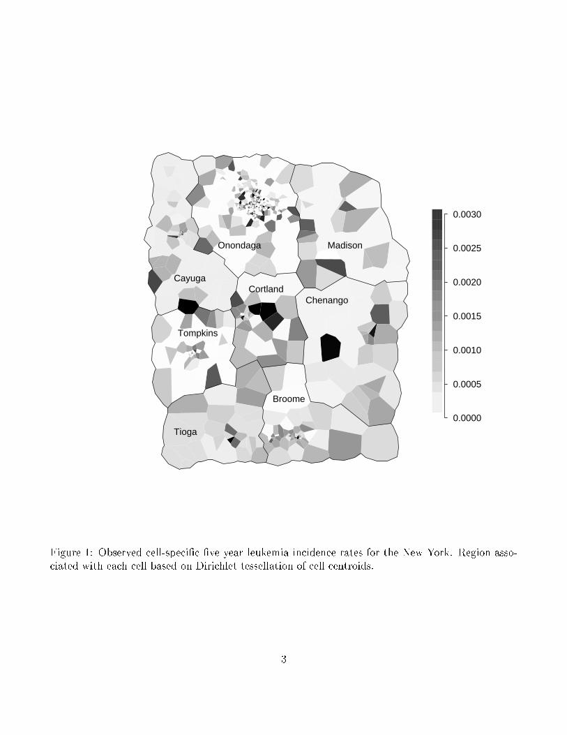
As an example, consider the well-known data set consisting of data on leukemia incidence for

a �ve-year period in an eight-county region of upstate New York. The observed leukemia rates for

census blocks (in seven counties) or tracts (in Broome county) are displayed in Figure 1. Waller

et al. (1994) provide additional background information about the New York leukemia data as well

as analyzes of these data using a number of cluster detection methods, including their own method

and the methods of Whittemore et al. (1987), Openshaw et al. (1988), Turnbull et al. (1990).

Kulldor� and Nagarwalla (1995) and Gangnon and Clayton (2001) later analyzed the New York

leukemia data using cluster detection methods they had developed.

Many Bayesian approaches to analyzing spatial disease patterns focus on mapping spatially

smoothed disease rates (for example, Clayton and Kaldor, 1987, Besag et al., 1991 and Waller et al.,

1997)). Mapping methods produce stable estimates for cell-speci�c rates by borrowing strength from

neighboring cells. These are most useful for capturing gradual, regional changes in disease rates, and

are less useful in detecting abrupt, localized changes indicative of hot spot clustering. The models

proposed by Besag et al. (1991) and Waller et al. (1997) incorporate both spatially structured

2

0.0000

0.0005

0.0010

0.0015

0.0020

0.0025

0.0030

Broome

Tioga

Tompkins

CortlandChenango

Cayuga

Onondaga Madison

Figure 1: Observed cell-speci�c �ve year leukemia incidence rates for the New York. Region asso-ciated with each cell based on Dirichlet tessellation of cell centroids.

3

(spatial correlation) and unstructured (extra-Poisson variation) heterogeneity in one model. The

ability of these models to detect localized clusters is questionable, because they incorporate only

a global clustering mechanism. In addition, typically, the spatially structured and unstructured

components of the heterogeneity are not separately identi�able by the likelihood (Waller et al.,

1997).

A few Bayesian approaches more directly address the disease clustering problem, including

Lawson (1995), Lawson and Clark (1999), Gangnon and Clayton (2000), Knorr-Held and Ra�er

(2000), Lawson (2000) and Denison and Holmes (2001). Lawson (1995) proposes a point process

model for detection of cluster locations when exact case (and control) locations are known. Lawson

(2000) describes an extension of this model to incorporate both localized clustering and general

spatial heterogeneity of disease rates. Lawson and Clark (1999) describe the application of a point

process clustering model to case count data through data augmentation. To apply their model,

one imputes locations for each member of the population at risk, typically by assuming a uniform

spatial distribution within each cell, to produce a point process. One then proposes a clustering

model for the point process.

Gangnon and Clayton (2000), Knorr-Held and Ra�er (2000) and Denison and Holmes (2001)

each consider a relatively nonparametric Bayesian framework for cluster detection in which cells are

grouped into clusters. A single, common rate for cells belonging to the same cluster is assumed.

The prior speci�cation of Gangnon and Clayton (2000) assumes a large background area and a

small number of clusters; the prior probability of a speci�c set of clusters is based on geographic

characteristics of the clusters such as their size and shape. The prior speci�cations of Knorr-Held

and Ra�er (2000) and Denison and Holmes (2001) assume clusters are de�ned by a set of cells

chosen as cluster centers (cells belong to the cluster associated with the nearest cluster center); the

prior probability of a set of clusters is based on a uniform selection of each cell as a cluster center.

All three methods provide very exible speci�cations of clusters. The approaches of Knorr-Held and

4

Ra�er (2000) and Denison and Holmes (2001) have some analytic advantages, while the approach

of Gangnon and Clayton (2000) more directly models the prior probability of particular clusters.

None of these methods include a spatial heterogeneity component in their model.

In this paper, we develop a Bayesian approach to inference about the parameters of a hierarchical

model for spatial clustering. This model includes both a discrete spatial clustering component and a

general spatial heterogeneity component to capture extra-Poisson variation. The model requires the

speci�cation of a set of potential clusters and a prior distribution on that set of potential clusters.

The proposed approach allows for multiple clusters and produces posterior estimates of cell-speci�c

and cluster-speci�c relative risks as well as cell-speci�c probabilities of cluster membership. In

addition, posterior inference about the number of clusters in the data is also possible, and estimates

are available both conditional on a �xed number of clusters and unconditionally.

In Section 2, we describe our hierarchical model for spatial clustering of disease rates, which

includes spatially unstructured random e�ects to capture extra-Poisson variation in the rates. In

Section 3, we describe our implementation of a reversible jump Markov chain Monte Carlo algorithm

(RJMCMC) (Green, 1995) sampler for drawing inferences about the model. In Section 4, we analyze

the aforementioned data on leukemia incidence in upstate New York using the proposed model.

Finally, in Section 5, we close with a discussion of alternative model speci�cations and extensions.

2 Statistical Model

We begin by de�ning some notation and a basic statistical model. We consider situations in which

the study region is divided into N subregions, or cells. For each cell i, we observe Oi, the number

of cases of disease, and ni, the population at risk in cell i. We assume a Poisson model for the data,

i.e., Oi � Poisson(�ini), where �i is the disease rate in cell i.

We model the cell-speci�c disease rates using a log-linear model log(�i) = �+Pk

j=1 �jIfi2cjg+ �i.

There are three basic components in this model: a non-spatial component (�), a spatial clustering

5

component (Pk

j=1 �jIfi2cjg), and a spatial heterogeneity (or extra-Poisson variation) component (�i).

Our primary interest lies in a prior speci�cation for the spatial clustering component of the model;

fairly standard priors are available for the other two components.

In our development here, the non-spatial component of the model consists of a single parameter

�. This parameter is related to the overall rate across the study region and is well-identi�ed by the

data. We propose using a at prior for this parameter (a normal prior with large variance serves

equally well). In other settings, the non-spatial component of the model could also incorporate the

e�ects of covariates such as age and sex.

For the spatial heterogeneity e�ects (�i), we follow other authors (cf. Waller et al. (1997)) in

proposing an exchangeable normal prior for the �i's; that is, �i � N(0; 1=�). For the parameter

� , we use a proper, but relatively weak, gamma prior distribution for � . In Section 4, a gamma

distribution with mean 1 and variance 1=4 is used.

The spatial clustering component of the model is based on the following parameters: k, the

number of clusters; c1; c2; : : : ; ck, the sets of cells belonging to the k clusters; and �1; �2; : : : ; �k,

the log relative risks associated with each cluster. We develop a prior for the spatial clustering

component of the model by successively conditioning on parameters. Given k; c1; c2; : : : ; ck (i.e.,

the number of clusters and their locations), we assign an exchangeable normal prior for �1; �2; : : : �k;

that is, �j � N(0; �2�). The prior variance �2� must be chosen in advance. Given the relatively

small number of clusters in most settings, the data will not provide enough information to reliably

estimate �2� . In the example, we take �2� to be 0:355 so that, a priori, the relative risk associated

with a cluster falls between 0.25 and 4.00 with 99% probability.

Next, given k (i.e., the number of clusters), we select c1; c2; : : : ; ck exchangeably (independently)

from a prior distribution on the space of possible clusters; denote this distribution by p(c). Note

that, under such a speci�cation, one of the clusters may overlap or, in the extreme, even duplicate

another cluster. To make this discussion more concrete, we consider a speci�c set of potential

6

clusters and develop a prior distribution for it. A similar development in a hypothesis testing

framework is described in Gangnon and Clayton (2001).

We consider circular clusters centered at the cell centroids as potential clusters. We center

clusters at the centroids to avoid empty clusters. The radius of the circles varies continuously

from zero up to a �xed maximum radius, rmax. If the centroid of a cell falls within the circle,

then the whole cell is included in the cluster. Since there are only a �nite number of cells, there

will only be a �nite number of clusters about each cell centroid. To identify these clusters, let

0 = ri;(1) < ri;(2) < : : : < ri;(mi) � rmax be the ordered distances from the centroid of cell i to the

centroids of all cells, truncated at rmax. (If two or more centroids are equidistant from the centroid

i, the common distance is only listed once.) Then, the distinct potential clusters about cell i are

circles of radii ri;(1); ri;(2); : : : ; ri;(mi). We refer to the cluster centered at the centroid of cell i of

radius ri;(j) as cluster i; j for j = 1; 2; : : : ; mi and i = 1; 2; : : : ; N .

Our prior distribution on the set of potential clusters is developed as and approximation to the

uniform selection of a cluster from the study region. Speci�cally, we �rst select a cluster center

and then, conditional on that center, select a cluster radius. We �rst select a point from a uniform

distribution over the study area and making the centroid of the cell to which the point belongs the

cluster center. The radius of the circle is then selected at random from a uniform distribution on

[0; rmax]. Thus, the prior probability of selecting cluster i; j is

p(i; j) =aiA�ri;j+1 � ri;j

rmax

,

where ai is the area of cell i, A is the area of the study region, and ri;mi+1 = rmax.

Finally, we select a prior distribution for k, the number of clusters. One possibility would be

distributions on the non-negative integers such as the Poisson, geometric, or negative binomial distri-

butions. Another possibility, which we generally prefer, is to restrict k to the values 0; 1; 2; : : : ; kmax

7

for some positive integer kmax. In most problems, selecting a maximum number of clusters kmax

should not be too diÆcult. In the example, we assign kmax = 10. On this restricted space, we

typically place a at (discrete uniform) prior distribution.

3 Posterior Calculation

If the clusters (both number and location) were �xed, simulation from the posterior using Markov

chain Monte Carlo techniques would be quite straightforward. The structure of the problem is that

of a hierarchical generalized linear model. Bayesian techniques for analyzing GLMs are discussed

in Gelman et al. (1995), and we follow their approach. The normal prior distributions for �,

�1; �2; : : : ; �k, and �1; �2; : : : ; �N are conjugate to a normal approximation to the Poisson likelihood.

For this normal approximation, we can easily �nd the full conditional distributions, and Gibbs

sampling would be appropriate. To correct for the approximation, the Gibbs sampler is used as a

proposal distribution in a Metropolis-Hastings algorithm (Hastings, 1970).

To make this discussion more concrete, we explicitly describe the Metropolis-Hastings steps for

updating �. To propose a new value for �, we need Ot (the total case count in the study region), Et

(the current value for the expected number of cases in the entire study region), and �0, the current

value for � in addition to the prior mean and variance for �, denoted by � and �2�. A proposed new

value of �, denoted �0, is drawn from a normal distribution with mean

�p =Et

Et + 1=�2��0 +

1=�2�Et + 1=�2�

� +Ot � Et

Et + 1=�2�

and variance

�2p =1

Et + 1=�2�.

8

The new value �0 is accepted with probability

min

8<:1; �(�; �

0p; �

2p

0)

�(�0; �p; �2p)

�(�0; �; �2�)

�(�; �; �2�)

l(Ot; E0t)

l(Ot; Et)

9=; ;

otherwise, the current value � is retained. In this equation, �(�; �; �2) is the density of a normal

random variable with mean � and variance �2 and l(y; �) is the likelihood of a Poisson random

variable with observed count y and mean �. The de�nitions of Metropolis-Hastings steps for the

other parameters �1; �2; : : : ; �k and �1; �2; : : : ; �N follow the same template.

The gamma prior distribution for � (the inverse of the prior variance for �1; �2; : : : ; �N) is also

conjugate, so samples for � can be obtained using the Gibbs sampler. To be concrete, if the

prior distribution for � follows a gamma(a; b) distribution (mean a=b and variance a=b2), the full

conditional distribution of � is gamma(a+N; b+PN

i=1 �i).

The novelty in the current problem is the unknown number (and locations) of the clusters. A

number of additional transitions must be proposed to account for the varying number of clusters. A

general approach to accounting for a varying numbers of parameters is the reversible jump Markov

chain Monte Carlo (RJMCMC) algorithm (Green, 1995).

In addition to the steps for �xed clusters described above, we propose the following three steps.

1. ADD: Propose a new cluster ck+1 and its associated parameter �k+1 for the model.

2. DROP: Propose a cluster to remove from the model.

3. CHANGE: Propose a new cluster location for a cluster currently in the model (maintaining

the same value for the associated �).

The ADD and DROP steps are counterparts of each other, while the CHANGE step is its own

counterpart. In each iteration of the algorithm, one of these three steps is proposed with probability

pa(k), pd(k) and pc(k) respectively. Note that these probabilities depend on the current value of the

9

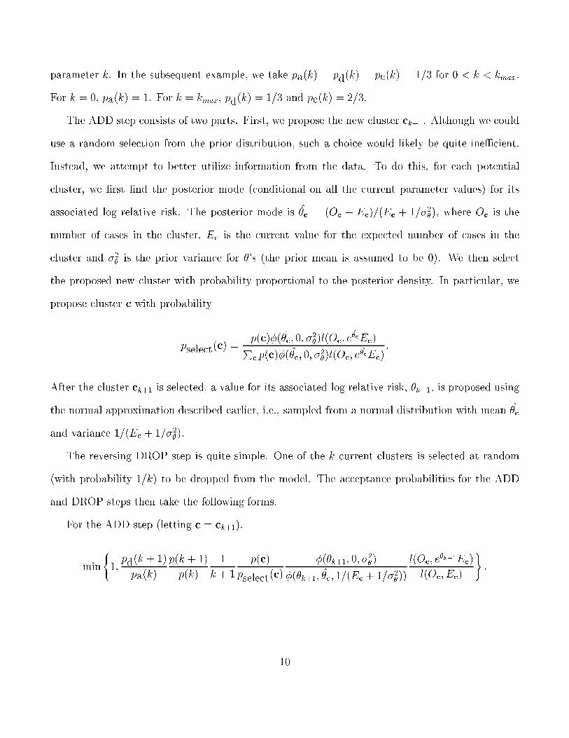
parameter k. In the subsequent example, we take pa(k) = pd(k) = pc(k) = 1=3 for 0 < k < kmax.

For k = 0, pa(k) = 1. For k = kmax, pd(k) = 1=3 and pc(k) = 2=3.

The ADD step consists of two parts. First, we propose the new cluster ck+1. Although we could

use a random selection from the prior distribution, such a choice would likely be quite ineÆcient.

Instead, we attempt to better utilize information from the data. To do this, for each potential

cluster, we �rst �nd the posterior mode (conditional on all the current parameter values) for its

associated log relative risk. The posterior mode is �̂c = (Oc � Ec)=(Ec + 1=�2�), where Oc is the

number of cases in the cluster, Ec is the current value for the expected number of cases in the

cluster and �2� is the prior variance for �'s (the prior mean is assumed to be 0). We then select

the proposed new cluster with probability proportional to the posterior density. In particular, we

propose cluster c with probability

pselect(c) =p(c)�(�̂c; 0; �

2�)l(Oc; e

�̂cEc)Pcp(c)�(�̂

c; 0; �2�)l(Oc

; e�̂cEc).

After the cluster ck+1 is selected, a value for its associated log relative risk, �k+1, is proposed using

the normal approximation described earlier, i.e., sampled from a normal distribution with mean �̂c

and variance 1=(Ec + 1=�2�).

The reversing DROP step is quite simple. One of the k current clusters is selected at random

(with probability 1=k) to be dropped from the model. The acceptance probabilities for the ADD

and DROP steps then take the following forms.

For the ADD step (letting c = ck+1),

min

(1;pd(k + 1)

pa(k)

p(k + 1)

p(k)

1

k + 1

p(c)

pselect(c)

�(�k+1; 0; �2�)

�(�k+1; �̂c; 1=(Ec + 1=�2�))

l(Oc; e�k+1Ec)

l(Oc; E

c)

).

10

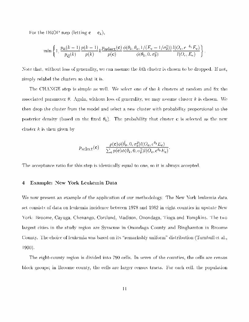
For the DROP step (letting c = ck),

min

(1;pa(k � 1)

pd(k)

p(k � 1)

p(k)kpselect(c)

p(c)

�(�k; �̂c; 1=(Ec + 1=�2�))

�(�k; 0; �2�)

l(Oc; e��kEc)

l(Oc; Ec)

).

Note that, without loss of generality, we can assume the kth cluster is chosen to be dropped. If not,

simply relabel the clusters so that it is.

The CHANGE step is simple as well. We select one of the k clusters at random and �x the

associated parameter �. Again, without loss of generality, we may assume cluster k is chosen. We

then drop the cluster from the model and select a new cluster with probability proportional to the

posterior density (based on the �xed �k). The probability that cluster c is selected as the new

cluster k is then given by

pselect(c) =p(c)�(�̂k; 0; �

2�)l(Oc

; e�kEc)P

cp(c)�(�k; 0; �2�)l(Oc; e�kEc)

.

The acceptance ratio for this step is identically equal to one, so it is always accepted.

4 Example: New York Leukemia Data

We now present an example of the application of our methodology. The New York leukemia data

set consists of data on leukemia incidence between 1978 and 1982 in eight counties in upstate New

York: Broome, Cayuga, Chenango, Cortland, Madison, Onondaga, Tioga and Tompkins. The two

largest cities in the study region are Syracuse in Onondaga County and Binghamton in Broome

County. The choice of leukemia was based on its \remarkably uniform" distribution (Turnbull et al.,

1990).

The eight-county region is divided into 790 cells. In seven of the counties, the cells are census

block groups; in Broome county, the cells are larger census tracts. For each cell, the population

11

at risk, count of leukemia cases and geographic centroid are available. A few cases could not be

assigned to a single cell due to incomplete location data. These cases are fractionally assigned to

the possible cells in proportion to the cell populations. Additional background information on the

New York leukemia data is available in Waller et al. (1994) and Gangnon and Clayton (2000). The

observed leukemia rate for each cell in Figure 1 using the Dirichlet tessellation of the cell centroids.

No obvious clusters are evident in this �gure. (Insertion point for Figure 1)

For our analysis of the New York leukemia data, we utilized the prior described in Section 2.

Following Gelman and Rubin (1992), we ran �ve independent Markov chains. Each chain used a

run-in of 10,000 iterations, and samples from the next 10,000 iterations were used for inference.

The chains appeared to converge by that point, and there were not substantial di�erences in the

samples across chains.

In Table 1, we present the posterior distribution of the number of clusters k included in the

model. Based on this distribution, there does not appear to be strong evidence about the correct

number of clusters in the model. A model with no clusters has a posterior probability of 0.10.

Higher posterior probabilities are associated with the one cluster (0.28), two cluster (0.32) and

three cluster (0.19) models. The posterior probability of a model with more than three clusters is

approximately 0.11. Thus, we have fairly strong evidence of clustering in the data, but equivocal

evidence for the correct number of clusters (1, 2, or 3).

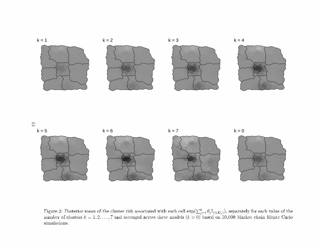
In Figure 2, we display the posterior means for the cluster risks associated with each cell

exp(Pk

j=1 �jIfi2cjg), separately for each value of the number of clusters k = 1; 2; : : : ; 7 and aver-

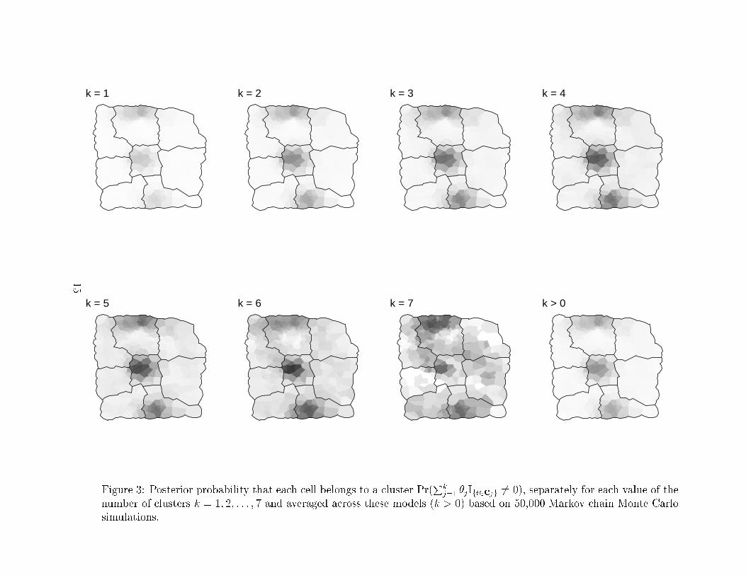
aged across these models (k > 0). In Figure 3, we display the posterior probability that a cell

belongs to a cluster Pr(Pk

j=1 �jIfi2cjg 6= 0), separately for each value of the number of clusters

k = 1; 2; : : : ; 7 and averaged across these models (k > 0).

These �gures show convincing evidence for three areas of clustering in the New York leukemia

data. The term \areas of clustering" is used instead of \clusters" to indicate that the data support

12

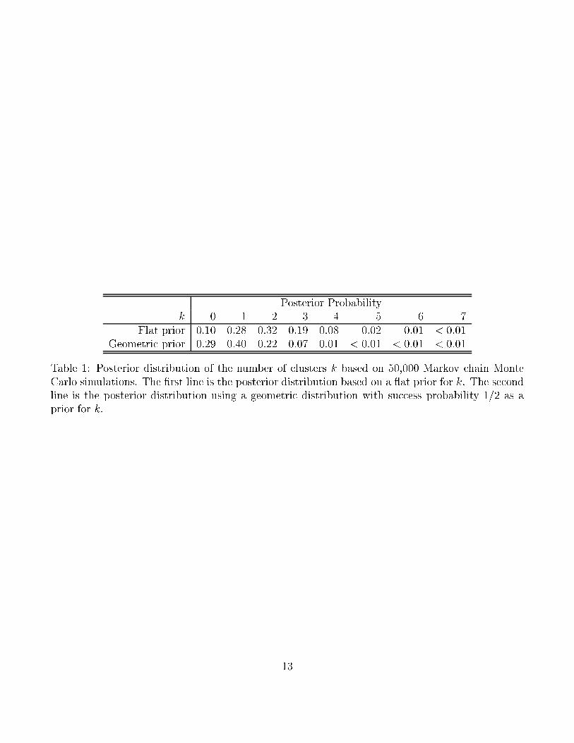
Posterior Probabilityk 0 1 2 3 4 5 6 7

Flat prior 0.10 0.28 0.32 0.19 0.08 0.02 0.01 < 0:01Geometric prior 0.29 0.40 0.22 0.07 0.01 < 0:01 < 0:01 < 0:01

Table 1: Posterior distribution of the number of clusters k based on 50,000 Markov chain MonteCarlo simulations. The �rst line is the posterior distribution based on a at prior for k. The secondline is the posterior distribution using a geometric distribution with success probability 1=2 as aprior for k.

13

k = 1 k = 2 k = 3 k = 4

k = 5 k = 6 k = 7 k > 0

Figure 2: Posterior mean of the cluster risk associated with each cell exp(Pk

j=1 �jIfi2cjg), separately for each value of the

number of clusters k = 1; 2; : : : ; 7 and averaged across these models (k > 0) based on 50,000 Markov chain Monte Carlo

simulations.

14

k = 1 k = 2 k = 3 k = 4

k = 5 k = 6 k = 7 k > 0

Figure 3: Posterior probability that each cell belongs to a cluster Pr(Pk

j=1 �jIfi2cjg 6= 0), separately for each value of the

number of clusters k = 1; 2; : : : ; 7 and averaged across these models (k > 0) based on 50,000 Markov chain Monte Carlo

simulations.

15

many di�erent speci�c clusters in a particular area. The �rst area of clustering is located in Broome

County in the southern portion of the study region and is associated with an increased leukemia

risk. This area includes the city of Binghamton. The second area of clustering is located in Cortland

County in the center of the study region and is also associated with an increased leukemia risk. The

third area of clustering is located in Onondaga County, north of Syracuse, and is associated with

a decreased risk of leukemia. As the number of clusters in the model increases, the estimated risks

or bene�ts associated with these clusters increases.

To summarize the risks associated with these apparent clusters, we use the posterior expected

risk associated with the cell in each area with the largest estimated probability of belonging to a

cluster. The estimated risk associated with the area of clustering in Cortland County is 1.40. The

estimated risk associated with the area of clustering in Broome County is 1.19. The estimated risk

associated with the area of clustering in Onondaga County is 0.81.

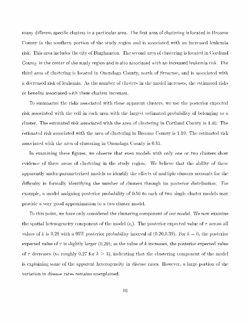
In examining these �gures, we observe that even models with only one or two clusters show

evidence of three areas of clustering in the study region. We believe that the ability of these

apparently under-parameterized models to identify the e�ects of multiple clusters accounts for the

diÆculty in formally identifying the number of clusters through its posterior distribution. For

example, a model assigning posterior probability of 0.50 to each of two single cluster models may

provide a very good approximation to a two cluster model.

To this point, we have only considered the clustering component of our model. We now examine

the spatial heterogeneity component of the model (�i). The posterior expected value of � across all

values of k is 0.28 with a 95% posterior probability interval of (0.20,0.39). For k = 0, the posterior

expected value of � is slightly larger (0.29); as the value of k increases, the posterior expected value

of � decreases (to roughly 0.27 for k � 3), indicating that the clustering component of the model

is explaining some of the apparent heterogeneity in disease rates. However, a large portion of the

variation in disease rates remains unexplained.

16

In Figure 3, we present the posterior means for the disease rate in each cell, �rst without a clus-

tering component (k = 0) and second with an unspeci�ed number of clusters (k > 0). Although the

two maps seem almost indistinguishable at a glance, some evidence of the three areas of clustering is

apparent upon study. For the representative cell in Cortland County, the posterior mean rate is 13.7

per 10,000 persons with a clustering component versus 11.4 per 10,000 persons without a clustering

component. For Broome County, the rates are 7.1 per 10,000 and 6.6 per 10,000, respectively. For

Onondaga County, the rates are 3.6 per 10,000 and 4.5 per 10,000 respectively.

In truth, a at prior on the number of clusters may be unrealistic. A more defensible prior

would likely place higher weight a priori on models with few clusters than on models with many

clusters. To illustrate the e�ects of such a prior choice on inference, we consider the impact of

assigning a geometric prior (with failure probability 1=2) to k. The posterior samples based on

the at prior provide an importance sample for the posterior based on the geometric prior; the

importance sampling weights for a model with k clusters is proportional to 0:5k. The posterior for

k based on this second prior is provided in Table 1. Compared with the posterior based on a at

prior, this distribution is shifted substantially towards models with k = 0; 1 or 2. There is little

support for a model with k > 3 (posterior probability < 0:10).

Despite this shift in the posterior for k, the resulting posterior for the cluster risks (and associated

probabilities of belonging to a cluster) still shows evidence of the three areas of clustering. Under

this posterior, the estimated risks associated with the representative cells described above are 1.31 in

Cortland County, 1.14 in Broome County and 0.83 in Onondaga County. This again demonstrates

the ability of the one and two cluster models to capture, at least partially, the risks associated with

three clusters.

Many previous analyses of the New York leukemia data have been published. Most of the

previous analyses have been based on hypothesis testing methods and solely aimed at detecting a

single cluster with an elevated risk of disease. These methods have generally detected clustering

17

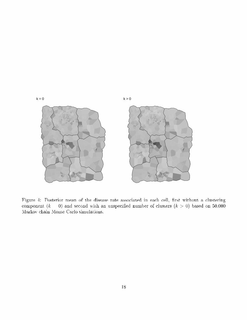
k = 0 k > 0

Figure 4: Posterior mean of the disease rate associated in each cell, �rst without a clusteringcomponent (k = 0) and second with an unspeci�ed number of clusters (k > 0) based on 50,000Markov chain Monte Carlo simulations.

18

in either Broome County or Cortland County (Waller et al., 1994). Some methods such as that

of Kulldor� and Nagarwalla (1995) showed evidence of clustering in both locations; however, they

provided no formal method for evaluating the signi�cance of multiple clusters.

An alternative Bayesian analysis of the New York leukemia data was described by Gangnon and

Clayton (2000). Their method allowed for a much larger class of potential clusters; essentially any

connected set of cells was a potential cluster. In contrast, the method described here uses a limited

set of potential clusters. The bene�ts of using a limited set of clusters include a more concrete prior

speci�cation (especially for the parameter k) and the ability to incorporate spatial heterogeneity

e�ects into the model.

Gangnon and Clayton (2000) found evidence for three clusters associated with an increased risk

of leukemia: areas of clustering in Broome and Cortland counties discussed here and an area of

clustering in Onondaga county within the city of Syracuse. The di�erences in inference likely result

from di�erences in prior speci�cations and the inclusion of a spatial heterogeneity component in

our model. The prior used in Gangnon and Clayton (2000) places relatively larger weight on the

many small, overlapping clusters within Syracuse than the more uniform prior used in our analysis.

A recent analysis by Denison and Holmes (2001) produced an estimated risk surface that shows

apparent evidence for all four features described above. They found compelling evidence for elevated

leukemia risks in Broome and Cortland counties, but did not present formal evaluations of the risks

in Onondaga county.

5 Discussion

In this paper, we demonstrate the use of a hierarchical model for estimating spatial clustering

and spatial heterogeneity e�ects in cell count data. The model for clustering e�ects assumes a

discontinuous risk surface with a large background region and a small number of clusters. The

model for heterogeneity e�ects incorporates non-localized extra-Poisson variation in disease rates.

19

In addition to formal posterior inference on the number of clusters, the explanatory power of the

clustering e�ects can be assessed by the percent reduction in the variance of the heterogeneity e�ects

associated with their inclusion. We conclude by brie y commenting on two extensions of this work.

In our presentation, we have focused on a \ at prior" for the clusters. Likewise, inference about

the possibility of certain prespeci�ed clusters can be evaluated using a \ at" prior for the clusters.

On the other hand, prior knowledge of cluster locations can be incorporated into these models in

one of two ways. An informative prior could be postulated for the �rst cluster. For example, with

probability one, the �rst cluster could be required to overlap a single cell (or a set of cells or one

of a set of cells). In such a setting, the �rst cluster would likely be forced into the model and

inference would range over cluster sizes from 1 up to kmax. Alternatively, if the presence of the

cluster was less certain, a mixture prior could be formulated for the clusters such that, with some

probability, a cluster is drawn from the restricted distribution above, otherwise, a cluster is drawn

from the \uniform" distribution. The extension of these ideas to multiple prespeci�ed clusters is

straightforward.

Finally, we note that, in many applications, it is useful to evaluate the clustering e�ects after

accounting for regional covariates such as demographic composition of the cells or average pollution

levels. Since the underlying model is a generalized linear model, the inclusion of such covariates is

quite straightforward. One would simply replace the parameter � with the linear predictor �+� 0x.

One could also easily extend the model to incorporate interactions between the covariate e�ects

and the clusters.

References

Besag, J., York, J. and Molli�e, A. (1991). Bayesian image restoration, with two applications in

spatial statistics (with discussion). Annals of the Institute of Statistical Mathematics 43, 1{59.

20

Clayton, D. and Kaldor, J. (1987). Empirical Bayes estimates of age-standardized relative risks for

use in disease mapping. Biometrics 43, 671{681.

Denison, D. and Holmes, C. (2001). Bayesian partitioning for estimating disease risk. Biometrics

57, 143{149.

Gangnon, R. E. and Clayton, M. K. (2000). Bayesian detection and modeling of spatial disease

clustering. Biometrics 56, 922{935.

Gangnon, R. E. and Clayton, M. K. (2001). A weighted average likelihood ratio test for spatial

clustering of disease. Statistics in Medicine To Appear.

Gelman, A., Carlin, J. B., Stern, H. S. and Rubin, D. B. (1995). Bayesian Data Analysis. Chapman

& Hall.

Gelman, A. and Rubin, D. (1992). Inference from iterative simulation using multiple sequences.

Statistical Science 7, 457{472.

Green, P. (1995). Reversible jump Markov chain Monte Carlo computation and Bayesian model

determination. Biometrika 82, 711{732.

Hastings, W. K. (1970). Monte Carlo sampling methods using Markov chains and their applications.

Biometrika 57, 97{109.

Knorr-Held, L. and Ra�er, G. (2000). Bayesian detection of clusters and discontinuites in disease

maps. Biometrics 56, 13{21.

Kulldor�, M. and Nagarwalla, N. (1995). Spatial disease clusters: Detection and inference. Statistics

in Medicine 14, 799{810.

Lawson, A. B. (1995). Markov chain Monte Carlo methods for putative pollution source problems

in environmental epidemiology. Statistics in Medicine 14, 2473{2486.

Lawson, A. B. (2000). Cluster modelling of disease incidence via RJMCMC methods: a comparative

evaluation. Statistics in Medicine 19, 2361{2375.

Lawson, A. B. and Clark, A. (1999). Markov chain Monte Carlo methods for putative sources

21

of hazard and general clustering. In Lawson, A. B., Bohning, D., Biggeri, A., Viel, J.-F. and

Bertollini, R., editors, Disease Mapping and Risk Assessment for Public Health, chapter 9. Wiley

WHO.

Openshaw, S., Craft, A. W., Charlton, M. and Birch, J. M. (1988). Investigation of leukaemia

clusters by use of a geographical analysis machine. Lancet 1, 272{273.

Turnbull, B. W., Iwano, E. J., Burnett, W. S., Howe, H. L. and Clark, L. C. (1990). Monitoring for

clusters of disease: Application to leukemia incidence in upstate New York. American Journal

of Epidemiology 132, S136{S143.

Waller, L. A., Carlin, B. P., Xia, H. and Gelfand, A. E. (1997). Hierarchical spatio-temporal

mapping of disease rates. Journal of the American Statistical Association 92, 607{617.

Waller, L. A., Turnbull, B. W., Clark, L. C. and Nasca, P. (1994). Spatial patten analyses to detect

rare disease clusters. In Lange, N., Ryan, L. and Billard, L., editors, Case Studies in Biometry,

pages 3{22. John Wiley and Sons, New York.

Whittemore, A., Friend, N., Brown, B. W. and Holly, E. A. (1987). A test to detect clusters of

disease. Biometrika 74, 31{35.

22