Technische Universit�at ChemnitzSonderforschungsbereich 393Numerische Simulation auf massiv parallelen RechnernMathias Meisel Arnd MeyerHierarchically PreconditionedParallel CG{Solvers with andwithout Coarse{Mesh{Solversinside FEAPPreprint SFB393/97-20Fakult�at f�ur MathematikTU Chemnitz-ZwickauD-09107 Chemnitz, FRG(0371)-531-2657 (fax)mathias.meisel@mathematik.tu-chemnitz.dehttp://www.tu-chemnitz.de/�mmeisel(0371)-531-4105arnd.meyer@mathematik.tu-chemnitz.dehttp://www.tu-chemnitz.de/�amey(0371)-531-2659Preprint-Reihe des Chemnitzer SFB 393SFB393/97-20 September 1997

Hierarchically Preconditioned Parallel CG{Solverswith and without Coarse{Mesh{Solvers insideFEAPMathias Meisel Arnd MeyerSeptember 30, 1997AbstractAfter some remarks on the parallel implementation of the Finite Element pack-age FEAP, our realisation of the parallel CG{algorithm is sketched. From atechnical point of view, a hierarchical preconditioner with and without addi-tional global crosspoint preconditioning is presented. The numerical proper-ties of this preconditioners are discussed and compared to a Schur{comple-ment{preconditioning, using a wide range of data from computations on tech-nical and academic examples from elasticity.Contents1 The parallelized FEAP{Version 12 The parallel conjugate gradients algorithm 23 Hierarchical preconditioning 33.1 The hierarchical list : : : : : : : : : : : : : : : : : : : : : : : : : : : : 33.2 The hierarchical preconditioner : : : : : : : : : : : : : : : : : : : : : 44 Coars grid preconditioning 54.1 The coarse grid matrix : : : : : : : : : : : : : : : : : : : : : : : : : : 64.2 The crosspoint solver : : : : : : : : : : : : : : : : : : : : : : : : : : : 75 Di�erent technologies for the global assembly 76 Comparison to the Schur complement CG 87 Numerical results 97.1 The model problems : : : : : : : : : : : : : : : : : : : : : : : : : : : 107.2 Grid geometry and preconditioning : : : : : : : : : : : : : : : : : : : 107.3 Comparison of the preconditioners : : : : : : : : : : : : : : : : : : : : 137.4 Di�erent crosspoint matrices : : : : : : : : : : : : : : : : : : : : : : : 220

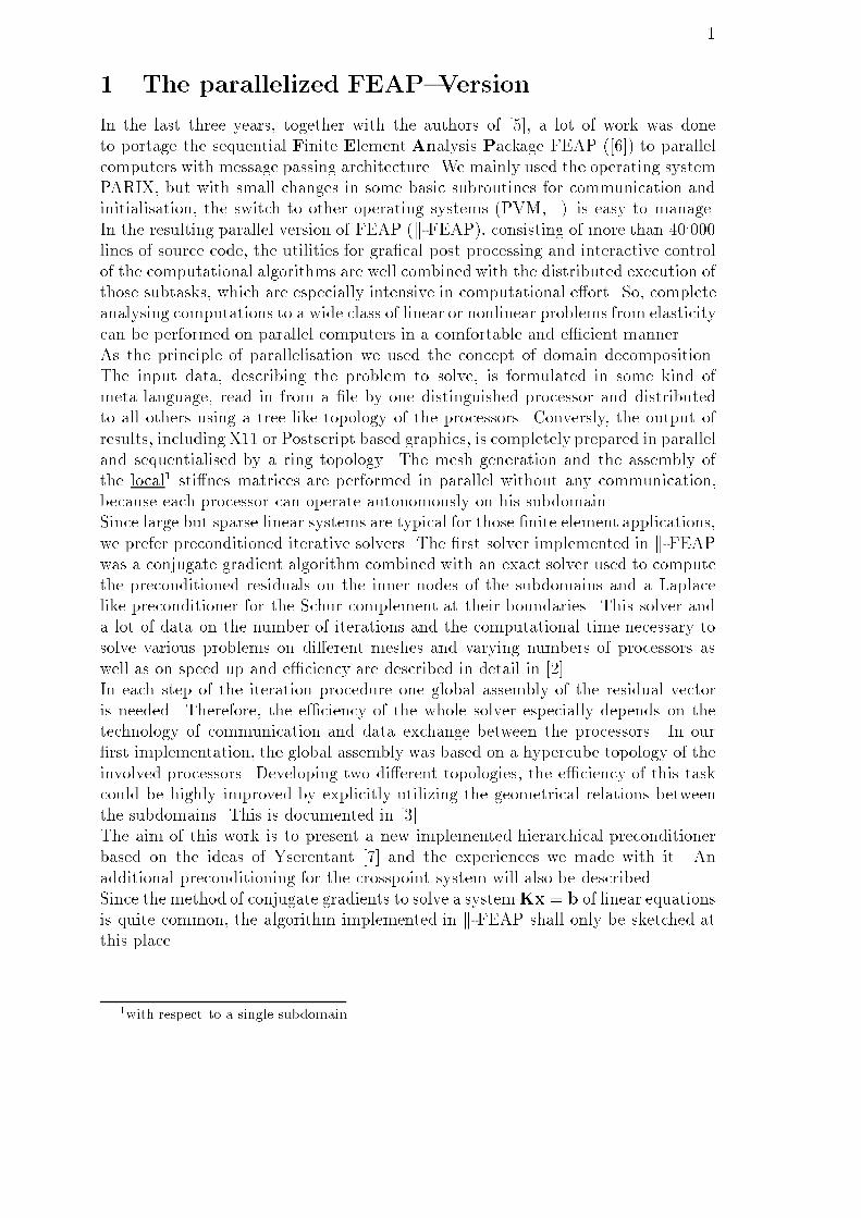
11 The parallelized FEAP{VersionIn the last three years, together with the authors of [5], a lot of work was doneto portage the sequential Finite Element Analysis Package FEAP ([6]) to parallelcomputers with message passing architecture. We mainly used the operating systemPARIX, but with small changes in some basic subroutines for communication andinitialisation, the switch to other operating systems (PVM,...) is easy to manage.In the resulting parallel version of FEAP (k-FEAP), consisting of more than 40:000lines of source code, the utilities for gra�cal post processing and interactive controlof the computational algorithms are well combined with the distributed execution ofthose subtasks, which are especially intensive in computational e�ort. So, completeanalysing computations to a wide class of linear or nonlinear problems from elasticitycan be performed on parallel computers in a comfortable and e�cient manner.As the principle of parallelisation we used the concept of domain decomposition.The input data, describing the problem to solve, is formulated in some kind ofmeta language, read in from a �le by one distinguished processor and distributedto all others using a tree like topology of the processors. Conversly, the output ofresults, including X11 or Postscript based graphics, is completely prepared in paralleland sequentialised by a ring topology. The mesh generation and the assembly ofthe local1 sti�nes matrices are performed in parallel without any communication,because each processor can operate autonomously on his subdomain.Since large but sparse linear systems are typical for those �nite element applications,we prefer preconditioned iterative solvers. The �rst solver implemented in k-FEAPwas a conjugate gradient algorithm combined with an exact solver used to computethe preconditioned residuals on the inner nodes of the subdomains and a Laplacelike preconditioner for the Schur complement at their boundaries. This solver anda lot of data on the number of iterations and the computational time necessary tosolve various problems on di�erent meshes and varying numbers of processors aswell as on speed up and e�ciency are described in detail in [2].In each step of the iteration procedure one global assembly of the residual vectoris needed. Therefore, the e�ciency of the whole solver especially depends on thetechnology of communication and data exchange between the processors. In our�rst implementation, the global assembly was based on a hypercube topology of theinvolved processors. Developing two di�erent topologies, the e�ciency of this taskcould be highly improved by explicitly utilizing the geometrical relations betweenthe subdomains. This is documented in [3].The aim of this work is to present a new implemented hierarchical preconditionerbased on the ideas of Yserentant [7] and the experiences we made with it. Anadditional preconditioning for the crosspoint system will also be described.Since the method of conjugate gradients to solve a systemKx = b of linear equationsis quite common, the algorithm implemented in k-FEAP shall only be sketched atthis place.1with respect to a single subdomain

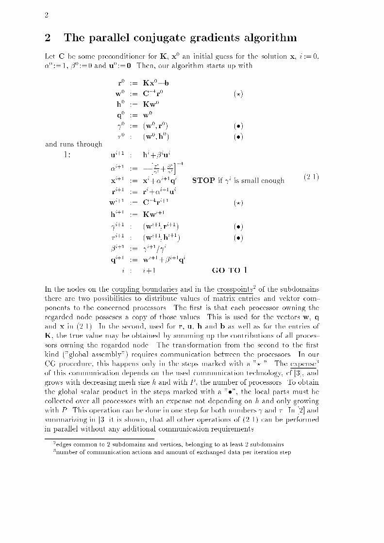
22 The parallel conjugate gradients algorithmLet C be some preconditioner for K, x0 an initial guess for the solution x, i := 0,�0 :=1, �0 :=0 and u0 :=0. Then, our algorithm starts up withr0 := Kx0�bw0 := C�1r0 (?)h0 := Kw0q0 := w0 0 := (w0; r0) (�)� 0 := (w0;h0) (�)and runs through1: ui+1 := hi+�iui�i+1 := � h � i i+ �i�i i�1xi+1 := xi+�i+1qi STOP if i is small enoughri+1 := ri+�i+1uiwi+1 := C�1ri+1 (?)hi+1 := Kwi+1 i+1 := (wi+1; ri+1) (�)� i+1 := (wi+1;hi+1) (�)�i+1 := i+1= iqi+1 := wi+1+�i+1qii := i+1 GO TO 1(2.1)

In the nodes on the coupling boundaries and in the crosspoints2 of the subdomainsthere are two possibilities to distribute values of matrix entries and vektor com-ponents to the concerned processors. The �rst is that each processor owning theregarded node posseses a copy of those values. This is used for the vectors w, qand x in (2.1). In the second, used for r, u, h and b as well as for the entries ofK, the true value may be obtained by summing up the contributions of all proces-sors owning the regarded node. The transformation from the second to the �rstkind ("global assembly") requires communication between the processors. In ourCG procedure, this happens only in the steps marked with a "? ". The expense3of this communication depends on the used communication technology, cf.[3], andgrows with decreasing mesh size h and with P , the number of processors. To obtainthe global scalar product in the steps marked with a "�", the local parts must becollected over all processors with an expense not depending on h and only growingwith P . This operation can be done in one step for both numbers and � . In [2] andsummarizing in [3] it is shown, that all other operations of (2.1) can be performedin parallel without any additional communication requirements.2edges common to 2 subdomains and vertices, belonging to at least 2 subdomains3number of communication actions and amount of exchanged data per iteration step

3The main disadvantages of using an exact solver to compute the preconditionedresiduum w at the inner nodes of the subdomains are the large amount of stor-age needed for the decomposed submatrices of K and the expense of arithmetic tocompute these factorization and the inner residuals.To overcome this, the hierarchical preconditioner presented in the following sectionwas implemented.3 Hierarchical preconditioningNeither the original version of FEAP nor the recent version of k-FEAP are designedto generate hierarchical meshes. Therefore, for meshes that could have been gener-ated by some hierarchical mesh generator, an algorithm for computing a hierarchicallist to such an existing mesh was implemented.3.1 The hierarchical listSuppose, the considered domain is decomposed into P quadrilateral subdomainss (0 � s � P �1) and these subdomains are distributed to P processors. As-sume, each processor Ps has generated a quadrilateral mesh on s, consisting of(2Nxs +1)�(2Nys +1) grid points. The totality of all these submeshes de�nes a FE{grid over without "hanging nodes". Then, k-FEAP is able to compute the hier-archical list for each subdomain in parallel and without communication, and theirtotality is a hierarchical list of the whole mesh.1 12 23 34 45 56 67 78 89 910 1011 1112 1213 1314 1421 2120 2019 1918 1817 1716 1615 1524 2423 2322 2225 2526 2627 2728 2829 2930 3031 3132 3233 3334 3435 3536 3637 3738 3839 3940 4041 4142 4243 4344 4445 450 0 00 0 01 11 12 2 2 2 23 3 3 33 3 3 33 3 3 344 44 44 44 44 44 44 44 445 5 5 5 5 5 5 55 5 5 5 5 5 5 55 5 5 5 5 5 5 55 5 5 5 5 5 5 55 5 5 5 5 5 5 5Figure 1: Example of a hierarchicalised mesh in 2 subdomainsIn �gure 1, the local numbering of the nodes used inside k-FEAP (above) and themembership of the nodes to the hierarchical levels (below) are displayed for the caseof 2 subdomains with Nx0 =Nx1 =3 and Ny0 =Ny1 =2.

4The main idea to get the hierarchical lists is the following:Let the boundary and the vertices of the subdomain (level 0) be �xed. Then,alternating in horizontal and vertical direction4, new lines are inserted, de�ning anew level, and the points of intersection with the just existing lines are added tothe hierarchical list at this new level als "sons" of the two nodes (fathers) in theneighbourhood on the intersected line.For each subdomain from �gure 1 this leads to the list presented in table 1.son father 1 father2 son father 1 father2 son father 1 father2level 1 level 4 5 1 68 1 2 22 4 23 19 18 2018 3 4 40 20 33 41 40 42level 2 42 18 35 34 33 3523 1 4 44 16 37 27 26 2835 8 18 14 3 13 7 6 813 2 3 24 1 23 17 16 18level 3 26 6 33 43 42 4420 4 18 28 8 35 36 35 3733 23 35 30 10 37 29 28 306 1 8 12 2 13 9 8 1016 3 18 level 5 15 3 1637 13 35 21 4 20 45 14 4410 2 8 39 22 40 38 13 3732 23 33 31 12 3025 24 26 11 2 10Table 1: Hierarchical list to �gure 13.2 The hierarchical preconditionerIn elasticity problems, there are typically I > 1 degrees of freedom associated to eachsingle node in the computational grid. They shall be numbered by i ; 1 � i � I,and the total number of unknowns is N :=I � p�1Ps=0 (2Nxs + 1)(2Nys + 1).Except the four vertices of the subdomain (level 0), each node in the hierarchi-cal(ized) mesh is the "son" of exactly two "fathers", cf. table 1, and for a meshconsisting of (2Nxs + 1) � (2Nys + 1) grid points the hierarchical list consists ofMs := (2Nxs +1)(2Nys +1) � 4 lines. Let these lines be numbered, starting fromthe lowest level 1 and ending at the highest level Nxs +Nys , with m ; 1 � m � Ms.With thist conventions, the notation Sm, F 1m and F 2m for the "son" and the two"fathers" in the m`th row of the hierarchical list is used to de�ne the linear operatorQs : viSm :=viSm+ 12 �viF 1m+viF 2m� ; i=1 (1) Im=1 (1) Ms (3.1)4in case of jNxs�Nys j > 1 in a more exible way to distribute the directions as evemly as possible

5acting on some grid function v, and it's transposedQTs : viF jm :=viF jm+ 12viSm ; j=1; 2i=1 (1) Im=Ms (�1) 1 : (3.2)In (3.1), the half of the sum of the values of both "fathers" is added to the value ofthe "son", whereas in (3.2) the half of the value of the \son\ is added to the valuesof both "fathers".As the collectivity of the local hierarchical lists de�nes the hierarchical list over thewhole domain, the local matrices Qs and QTs de�ne the two parts Q and QT of thehierarchical preconditioner over the whole grid.Since nodes with essential boundary conditions cannot be removed from the gridand the preconditioned residual wi has to be zero for all times whenever the initialsolution ful�lls this conditions, we need the diagonal matrix of dimension N:= diag (ll ) :=( 0 essential conditions1 all others (3.3)to cut o� pollutions. The matrixJ := diag (k�1ll ) (3.4)of the same dimension and derived from the sti�ness matrix K is needed to de-scribe an additional Jacobi scaling. Finally let � denote the operation of the globalassembly of a vector (cf. section 5).Then, the hierarchical preconditioner C in (2.1) may be expressed by5C�1 :=Q � J QT : (3.5)Except the assembly �, all operations in (3.5) can be performed in parallel andwithout communication.Applying or J to a vector is realized with the multiplication in components of twolocal vectors using standard routines described in [1], and Q as well as QT containonly simple operations acting on the same local vector.4 Coars grid preconditioningRegarding the loaded beam from �gure 3, divided into 128 subdomains and dis-tributet to 128 processors, we state, that only the subdomains s ; 96 � s � 127 ;are subject to the loading and no other than 0 contains essential boundary con-ditions. Since, in each CG{step, exchange of information takes place only acrossthe coupling boundaries between geometrically neighbouring subdomains, it takes5The rightmost can be dropped, if K contains no other than diagonal entries in the rowsassociated to essential boundary conditions.

6at least 96 steps until processor P0 gets some knowledge about the existence of theloading, and additional 127 steps are necessary to bring the �rst reaction forces fromo to P127`s attention.This heuristic considerations explain, why computations to the beam problem re-quire, by the same number of degrees of freedom, essentially more iterations thanthe geometrically more compact problem from �gure 2, when a large number ofprecessors is used6.The main idea of coarse grid preconditioning consists in regarding the domain de-composition as a computational grid and solving a suitable boundary value problem(BVP) on this grid to obtain improved residuals in the crosspoints. This BVP canbe the original problem or a substitute with similar properties.4.1 The coarse grid matrixIn case of quadrilateral subdomains, the most simple but in common use variant ofconstructing a coarse grid matrix is to regard the quadrilaterals as unit squares7 andassemble the descrete Laplacian over this uniform grid. The resulting matrix shallbe refered to by eLS . This requires no local computations and only a minimum ofstorage and communication, but the more the real geometry of the s di�ers fromsquares, the less is the coincidence to the original problem (cf. sections 7.4 and 7.2).To overcome this, the Matrix eLQ, arising from the global assembly of the descreteLaplacian over the real quadrilateral grid, takes presedence. The storage and com-munication requirements are the same as for eLS and so are the dimension and thebandwidth of the matrices. Because the geometrical computations must be per-formed only once bevor the iteration starts, the local computational e�ort can beleft out of account.Since the discrete Laplacians eLS or eLQ will be used separately for each of the Idegrees of freedom associated to a single node in the grid, the coarse grid matricesLS and LQ are de�ned to be the block diagonal matrices consisting of I eLS { oreLQ {blocks, respectively.The most expensive variant is to discretize the original problem on the coarse grid.In case of I > 1 degrees of freedom per single node, the dimenson of the resultingmatrices ES or EQ is the same as the dimension of LS, but they are less sparse,their bandwith is larger and they do not decompose into I submatrices independentfrom each other.Since a direct solver shall be used to solve the crosspoint problem, the matrix LQseems to be a good compromise.In k-FEAP, eLQ is gained by discretising the Laplace operator with bilinear functionsover all s and performing a global assembly on each Ps (cf. section 5). After that,each processor Ps performs a Cholesky decomposition with its own copy of eLQ,6With the preconditioner (3.5) inside the algorithm (2.1) on 128 processors, 837 iterationswere needed to solve the beam problem with 143550 degrees of freedom (dof), whereas thewedge problem with 143088 dof was solved after 136 steps.7e.g., neglecting the real geometry

7implicitly de�ning a decomposition for LQ:eLQ = eL eLT ; LQ = L LT : (4.1)4.2 The crosspoint solverWith the coarse grid matrix LQ (or LS) from the previous section, I being the unitmatrix of dimension N �NC , NC beeing the dimension of L,G�1 := L�1Q 00 I ! = (LT )�1L�1 00 I ! (4.2)and using Q, QT , �, and J from (3.1){(3.4), the hierarchical preconditioner withimbedded crosspoint preconditioning reads8C�1 := Q J1=2 G�1� J1=2 QT : (4.3)As in (3.5), the simple operations denoted by , QT , J1=2 and Q work in parallel andrequire no communication. Compared to (3.5), some additional communicationale�ort araises from the crosspoint solver, but this shall be diskussed in section 5.The root J1=2 should be precomputed before the iteration cycle starts. So, in com-parison to (3.5), the additional numerical e�ort per iteration step caused by thecrosspoint preconditioning is one diagonal scaling (J1=2) and I times the backwardand the forward substitution associated to (eLT )�1 eL�1.That's the reason why the pre-conditioning (4.3) actually requires less steps of iteration than (3.5) but sometimesneeds more computational time, when only a few steps are saved.5 Di�erent technologies for the global assemblyIn [3], three di�erent techniques for the assembly of the residuals in each CG{stepwere discussed in detail.On the �rst and simpliest, basing on the routine \cube{cat\ from [1] and referred toas \hypercube communication\, each processor collects the data from all couplingnodes9 of all other processors, seeks in the resulting storage vector10 for componentsrelated to nodes owned by himself, too, and ignores the rest. Obviously, especiallywhen a large number of processors is used, each processor uses only a small part ofthe interchanged data for the assembly of his residual values.To reduce this overhead, the \coupling{edges communication\ was developed. Onthis method, hypercube communication takes place only for the crosspoints, whereasthe data along the interior of each coupling edge is exchanged directly between thetwo processors, whose subdomains share this edge. This requires the generation of8footnote 5 from page 5 also applies to 4.39crosspoints and nodes at the coupling boundaries10which might be huge in case of a small meshsize and/or a large number of processors

8a virtual topology of the processors, re ecting the geometrical interrelationship ofthe subdomains.For domain decompositions consisting of quadrilaterals only, this topology consistsof up to 4 additional virtual links per processor.If the quadrilateral subdomains de�ne a tensor product mesh, a third technologynamed "crosspoint communication", uses no hypercube communication at all. In-cluding the crosspoint data at the end of the coupling edges into the direct dataexchange between the concerned processors, it remains to establish at each proces-sor again up to 4 additional virtual links to those processors, whose subdomainsintersect with the regarded subdomain in exactly one crosspoint, to exchange thecrosspoint data with all processors needing them. The larger the number of usedprocessors, the larger is the gain in time and storage.If no coarse grid preconditioning is intended (C�1 from (3.5)), crosspoint commu-nication is the most e�cient technology, because of the fewest storage requirementsand the least amount of transported data, but if C�1 shall be taken from (4.3), atleast one processor must collect all crosspoint data to solve the coarse grid system.There are two possibilities in common use:1. Only one processor assembles the coarse grid matrix, collects all coarse gridresiduals, solves the crosspopint system and distributes the solution to all otherprocessors. This works good with the routines like \tree{up\ and \tree{down\from [1].2. Each processor assembles his own coarse grid matrix, receives all coarse gridresiduals, solves the crosspopint system and uses only those components ofthe resulting vector, assigned to the edges of his own patch. In this case,\cube{cat\ should be used for the crosspoint data.In k-FEAP, the following is implemented: If the preconditioner (3.5) is used, theassembly of the residuals is based on \crosspoint communication\, and in case of(4.3), the \coupling{edges communication\ is choosen to meet the needs of thecrosspoint solver in variant 2. Note, that an additional crosspoint solver causesnot only additional numerical work per iteration step but also additional e�ort incommunication.6 Comparison to the Schur complement CGThe Schur complement CG algorithm (SCCG) is completly documented in [3], page5, or in [2].The essential computational expense per iteration consists of four linear combina-tions of vectors (y+tz), one matrix{vector{multiplication (Ky), two scalar products((x; y)) and the work to be done in the preconditioner (w = C�1r).To compare both algorithms from a local point of view, let N Is and NBs denote thenumber of degrees of freedom located in the interior and at the boundary of thesubdomain s.

9In [2] for the SCCG it was shown that, due to the exact solver used as precondi-tioner in the interior of the subdomains, all the four operations y + tz and the twoscalar products can be restricted to the nBs components associated to the couplingboundaries, saving 12N Is FLOP's in each step of the algorithm. For the same reason,instead of the whole matrix{vector{multiplication Ksws needed in the hierarchicalcase, only the submatrices KBs , KIBs and KBIs from Ks = � KBs KBIsKIBs KIs � must beapplied, saving at least additional 10N Is FLOP's. On the other hand, the numberof nonzero entries in the Cholesky factorization of KIs used in the SCCG growsquadratically with N Is , overcompensating the saved 22N Is FLOP's for su�cientlylarge problems.7 Numerical resultsTo compare the e�ciency of the various preconditioners, the following three exam-ples will be regarded. They are choosen to be at least a little bit realistic and,coincidental, make visible the expected bene�ts and disadvantages of the comparedalgorithms.The following abbreviations will be used in this chapter:� Ta and Tt are denoting the time needed for the arithmetic operations and thetotal time (including the time for communication).� T s, T h and T hc are denoting the time in seconds, needed to solve the prob-lem with SCCG, with the hierarchical preconditioner (3.5) and with thehierarchical preconditioner with additional crosspointsolver (4.3).� #s, #h and #hc are denoting the corresponding number of performed iterationsto achieve the desired accuracy ( i � 10�12 0 in (2.1)).� #hcS indicates, that the coarse grid matrix was based on eLS (see chapter 4.1).� DIM denotes the total size of the problem, counting unknowns located atcoupling nodes only once and reduced by the number of essential boundaryconditions.� P denotes the number of used processors.All computations were performed on the "GC{PowerPlus"{computer under thePARIX environment.

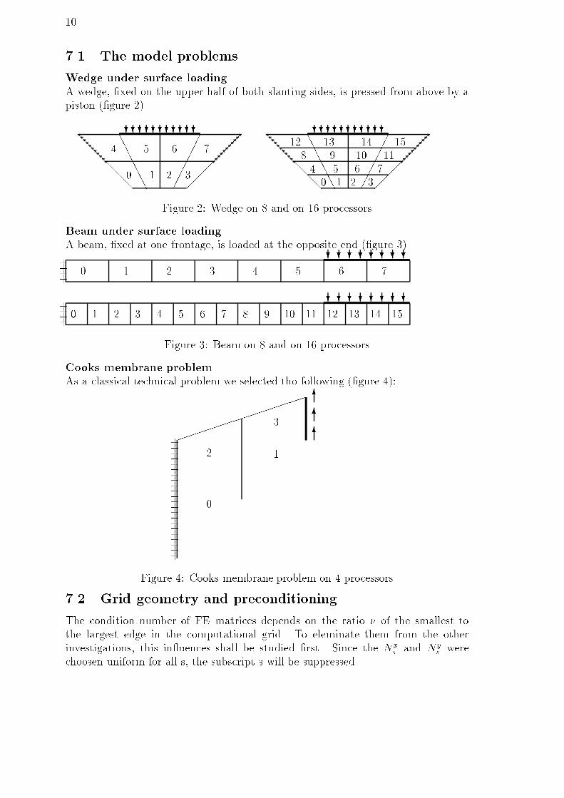
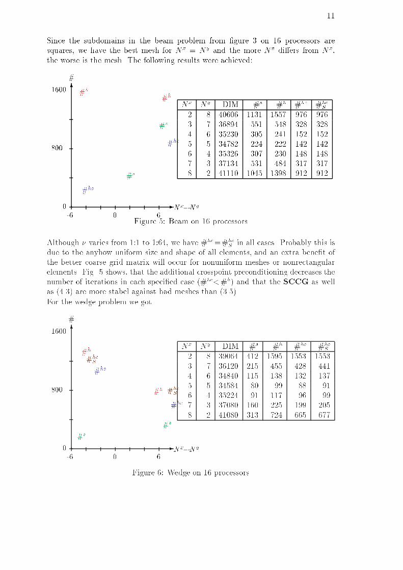
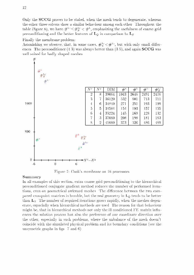
107.1 The model problemsWedge under surface loadingA wedge, �xed on the upper half of both slanting sides, is pressed from above by apiston (�gure 2). ������@@@@@@???????????AAAAAA ������ ������@@@@@@???????????AAAAAA ������0 1 2 34 5 6 7 0 1 2 34 5 6 78 9 10 1112 13 14 15Figure 2: Wedge on 8 and on 16 processorsBeam under surface loadingA beam, �xed at one frontage, is loaded at the opposite end (�gure 3).0 1 2 3 4 5 6 7 8 9 10 11 12 13 14 150 1 2 3 4 5 6 7????????????????++++++++ Figure 3: Beam on 8 and on 16 processorsCooks membrane problemAs a classical technical problem we selected tho following (�gure 4):��������������..................................................................................................................................................................................................................................................................................................................................................................................................

............................................................................................................................................................................................................................................................................................... 666++++++++++++++++++++++ 02 13Figure 4: Cooks membrane problem on 4 processors7.2 Grid geometry and preconditioningThe condition number of FE{matrices depends on the ratio � of the smallest tothe largest edge in the computational grid. To eleminate them from the otherinvestigations, this in uences shall be studied �rst. Since the Nxs and Nys werechoosen uniform for all s, the subscript s will be suppressed.

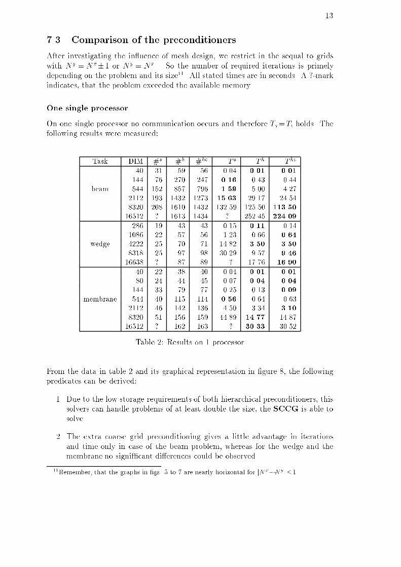
11Since the subdomains in the beam problem from �gure 3 on 16 processors aresquares, we have the best mesh for Nx = Ny and the more Nx di�ers from Nx,the worse is the mesh. The following results were achieved:Nx Ny DIM #s #h #hc #hcS2 8 40606 1131 1557 976 9763 7 36894 551 548 328 3284 6 35230 305 241 152 1525 5 34782 224 222 142 1426 4 35326 307 230 148 1487 3 37134 531 484 317 3178 2 41110 1045 1398 912 912Nx�Ny#-6 0 608001600

-6 #s#s.......................................................................................................................................................................................................................................................................................................................................................................................................................................................................................................................................................................................................................................................................................................................................................................................................................................................................

#h#h...................................................................................................................................................................................................................................................................................................................................................................................................................................................................................................................................................................................................................................................................................................................................................................................................................................................................................................................................................................................................................................................................................................................................................................................................... #hc#hc...............................................................................................................................................................................................................................................................................................................................................................................................................................................................................................................................................................................................................................................................................................................................................................................................................................................................................Figure 5: Beam on 16 processorsAlthough � varies from 1:1 to 1:64, we have #hc=#hcS in all cases. Probably this isdue to the anyhow uniform size and shape of all elements, and an extra bene�t ofthe better coarse grid matrix will occur for nonuniform meshes or nonrectangularelements. Fig. 5 shows, that the additional crosspoint preconditioning decreases thenumber of iterations in each speci�ed case (#hc<#h) and that the SCCG as wellas (4.3) are more stabel against bad meshes than (3.5).For the wedge problem we got Nx Ny DIM #s #h #hc #hcS2 8 39064 412 1595 1553 15533 7 36120 215 455 428 4414 6 34840 115 138 132 1375 5 34584 80 99 88 916 4 35224 91 117 96 997 3 37080 160 225 199 2058 2 41080 313 724 665 677Nx�Ny

#-6 0 608001600

-6

#s#s......................................................................................................................................................................................................................................................................................................................................................................................................................................................................................................................................#h #h................................................................................................................................................................................................................................................................................................................................................................................................................................................................................................................................................................................................................................................................................................................................................................................................................................................................................................................................................................................................................................................................ #hcS#hcS........................................................................................................................................................................................................................................................................................................................................................................................................................................................................................................................................................................................................................................................................................................................................................................................................................................................................................................................................................................................................................................ #hc#hc.......................................................................................................................................................................................................................................................................................................................................................................................................................................................................................................................................................................................................................................................................................................................................................................................................................................................................................................................................................................................................................................Figure 6: Wedge on 16 processors

12Only the SCCG proves to be stabel, when the mesh tends to degenerate, whereasthe other three solvers show a similar behaviour among each other. Throughout thetable (�gure 6), we have #hc�#hcS < #h, emphasizing the usefulness of coarse gridpreconditioning and the better features of LQ in comparison to LS .Finally the membrane problem:Astonishing we observe, that, in some cases, #hcS <#hc, but with only small di�er-ences. The preconditioner (4.3) was always better than (3.5), and again SCCG waswell suited for badly shaped meshes. Nx Ny DIM #s #h #hc #hcS2 8 39064 1043 2646 2491 24763 7 36120 532 801 713 7114 6 34840 271 251 193 1995 5 34584 154 193 157 1556 4 35224 145 169 128 1327 3 37080 208 198 181 1838 2 41080 373 526 486 489Nx�Ny

#

-6 0 608001600-

6#s#s.................................................................................................................................................................................................................................................................................................................................................................................................................................................................................................................................................................................................................................................................................................#h

#h....................................................................................................................................................................................................................................................................................................................................................................................................................................................................................................................................................................................................................................................................................................................................................................................................................................................................................................................................................................................................................................................................................................................................................................................................................................................................................................................................................... #hcS#hcS................................................................................................................................................................................................................................................................................................................................................................................................................................................................................................................................................................................................................................................................................................................................................................................................................................................................................................................................................................................................................................................................................................................................................................................................................................................................................................... #hc

#hc...........................................................................................................................................................................................................................................................................................................................................................................................................................................................................................................................................................................................................................................................................................................................................................................................................................................................................................................................................................................................................................................................................................................................................................................................................................................................................................................Figure 7: Cook's membrane on 16 processorsSummaryIn all examples of this section, extra coarse grid preconditioning to the hierarchicalpreconditioned conjugate gradient method reduces the number of performed itera-tions, even on geometrical awkward meshes. The di�erence between the two com-pared crosspoint matrices is humble, but the real geometry in LQ tends to be betterthan LS. The number of required iterations grows rapidly, when the meshes degen-erate, espacially when hierarchical methods are used. The reason for that behaviourmight be, that in hierarchical methods not only the ill conditioned FE{matrix in u-ences the solution process but also the preference of one coordinate direction overthe other, especially in such problems, where the unbalance of the mesh doesn'tcoincide with the simulated physical problem and its boundary conditions (see theunsymetric graphs in �gs. 7 and 6).

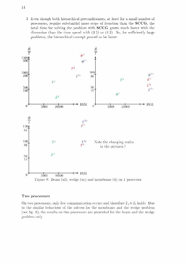
137.3 Comparison of the preconditionersAfter investigating the in uence of mesh design, we restrict in the sequal to gridswith Ny = Nx�1 or Ny = Nx . So the number of required iterations is primelydepending on the problem and its size11. All stated times are in seconds. A ?-markindicates, that the problem exceeded the available memory.One single processorOn one single processor no communication occurs and therefore Ta=Tt holds. Thefollowing results were measured:Task DIM #s #h #hc T s Th Thc40 31 59 56 0.04 0.01 0.01144 76 270 247 0.16 0.43 0.44beam 544 152 857 796 1.59 5.00 4.272112 193 1432 1273 15.63 29.17 24.548320 208 1610 1432 132.59 125.50 113.5016512 ? 1613 1434 ? 252.45 224.09286 19 43 43 0.15 0.11 0.141086 22 57 56 1.23 0.66 0.64wedge 4222 25 70 71 14.82 3.50 3.508318 25 97 98 30.29 9.57 9.4616638 ? 87 89 ? 17.76 16.9040 22 38 40 0.04 0.01 0.0180 24 44 45 0.07 0.04 0.04144 33 79 77 0.25 0.13 0.09membrane 544 40 115 114 0.56 0.64 0.632112 46 142 136 4.50 3.34 3.108320 51 156 159 44.89 14.77 14.8716512 ? 162 163 ? 30.33 30.52Table 2: Results on 1 processorFrom the data in table 2 and its graphical representation in �gure 8, the followingpredicates can be derived:1. Due to the low storage requirements of both hierarchical preconditioners, thissolvers can handle problems of at least double the size, the SCCG is able tosolve.2. The extra coarse grid preconditioning gives a little advantage in iterationsand time only in case of the beam problem, whereas for the wedge and themembrane no signi�cant di�erences could be observed.11Remember, that the graphs in �gs. 5 to 7 are nearly horizontal for jNx�Nyj�1.

14 3. Even though both hierarchical preconditioners, at least for a small number ofprocessors, require substantial more steps of iteration than the SCCG, thetotal time for solving the problem with SCCG grows much faster with thedimension than the time spend with (3.5) or (4.3). So, for su�ciently largeproblems, the hierarchical concept proved to be faster.DIM

#T0 5000 1000050010010002001500300

-6

#s......................................................................................................................................................................................................................................................T s..................................................................................................................................................................................................................................................................................................................#h

...........................................................................................................................................................................................................................................................................................................................................................................................................................................................................................................................................................................................................................................................................................................................................Th..........................................................................................................................................................................................................................................................................................................................................................................................................................................................................................................................................................................

#hc........................................................................................................................................................................................................................................................................................................................................................................

.............................................................................................................................................................................................................................................................................................................................T hc....................................................................................................................................................................................................................................................................................................................................................................................................................................................................................................................................................... DIM#T0 5000 10000153010050 -6 #s..................................................................................................................................................................................................................................................................................................................................................................................................T s............................................................................................................................................................................................................................................................................................................................................................................................................................................................................................................................................................................................................... #h................................................................................................................................................................................................................................................................................................................................................................................................................................................................................................................................................................................................................................................................................................................................................................................................................................................................................................................................................Th............................................................................................................................................................................................................................................................................................................................................................................................................................................................................................................................................................................................................................................................................................................................................................................................................................................................................ #hc................................................................................................................................................................................................................................................................................................................................................................................................................................................................................................................................................................................................................................................................................................................................................................................................................................................................................................................................................Thc........................................................................................................................................................................................................................................................................................................................................................................................................................................................................................................................................................................................................................................................................................................................................................................................................................................................................Note the changing scalesin the pictures !DIM

#T0 5000 1000015304515010050 -6 #s.....................................................................................................................................................................................................................................................................................................................................................................................................................................................................................T s.....................................................................................................................................................................................................................................................................................................................................................................................................................................................................................................................................................................................................................................................................................................................................................................................................................................

................................................ #h.................................................................................................................................................................................................................................................................................................................................................................................................................................................................................................................................................................................................................................................................................................................................................................................................................................................................................................................................................................................................................................................................................................................................................................................................................................................................................................................Th.................................................................................................................................................................................................................................................................................................................................................................................................................................................................................................................................................................................................................................................................................................................................................................................#hc

.............................................................................................................................................................................................................................................................................................................................................................................................................................................................................................................................................................................................................................................................T hc.....................................................................................................................................................................................................................................................................................................................................................................................................................................................................................................................................................Figure 8: Beam (ul), wedge (ur) and membrane (d) on 1 processorTwo processorsOn two processors, only few communication occurs and therefore Ta�Tt holds. Dueto the similar behaviour of the solvers for the membrane and the wedge problem(see �g. 8), the results on two processors are presented for the beam and the wedgeproblem only.

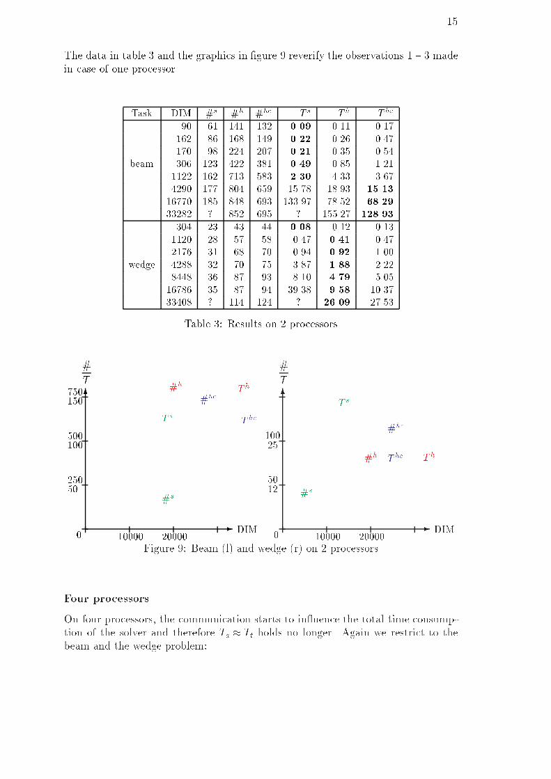
15The data in table 3 and the graphics in �gure 9 reverify the observations 1 { 3 madein case of one processor.Task DIM #s #h #hc T s T h Thc90 61 141 132 0.09 0.11 0.17162 86 168 149 0.22 0.26 0.47170 98 224 207 0.21 0.35 0.54beam 306 123 422 381 0.49 0.85 1.211122 162 713 583 2.30 4.33 3.674290 177 804 659 15.78 18.93 15.1316770 185 848 693 133.97 78.52 68.2933282 ? 852 695 ? 155.27 128.93304 23 43 44 0.08 0.12 0.131120 28 57 58 0.47 0.41 0.472176 31 68 70 0.94 0.92 1.00wedge 4288 32 70 75 3.87 1.88 2.228448 36 87 93 8.10 4.79 5.0516786 35 87 94 39.38 9.58 10.3733408 ? 114 124 ? 26.09 27.53Table 3: Results on 2 processorsDIM

#T0 10000 20000

75050025050100150-

6 #s.........................................................................................................................................................................................................................................................................................................................................................................................................................................................................................T s.................................................................................................................................................................................................................................................................................................................................................................................................... #h

.................................................................................................................................................................................................................................................................................................................................................................................................................................................................................................................................................................................................................................................................................................................................................................................................................................................................................................................................................................................................................................................................................................................................................................................................Th

........................................................................................................................................................................................................................................................................................................................................................................................................................................................................................................................................#hc...............................................................................................................................................................................................................................................................................................................................................................................................................................................................................................................................................................................................................................................................................................................................................................................................................................................................................................................................................................................................................................................................................................T hc...............................................................................................................................................................................................................................................................................................................................................................................................................................................................................................

.......DIM

#T0 10000 20000122510050 -6 #s..........................................................................................................................................................................................T s..................................................................................................................................................................................................................................................................................................................................

................................................................. #h................................................................................................................................................................................................................................................................................................................................................................................................Th............................................................................................................................................................................................................................................................................................................................................................................................................................#hc........................................................................................................................................................................................................................................................................................................................................................................................................Thc..................................................................................................................................................................................................................................................................................................................................................................................................................................Figure 9: Beam (l) and wedge (r) on 2 processorsFour processorsOn four processors, the communication starts to in uence the total time consump-tion of the solver and therefore Ta � Tt holds no longer. Again we restrict to thebeam and the wedge problem:

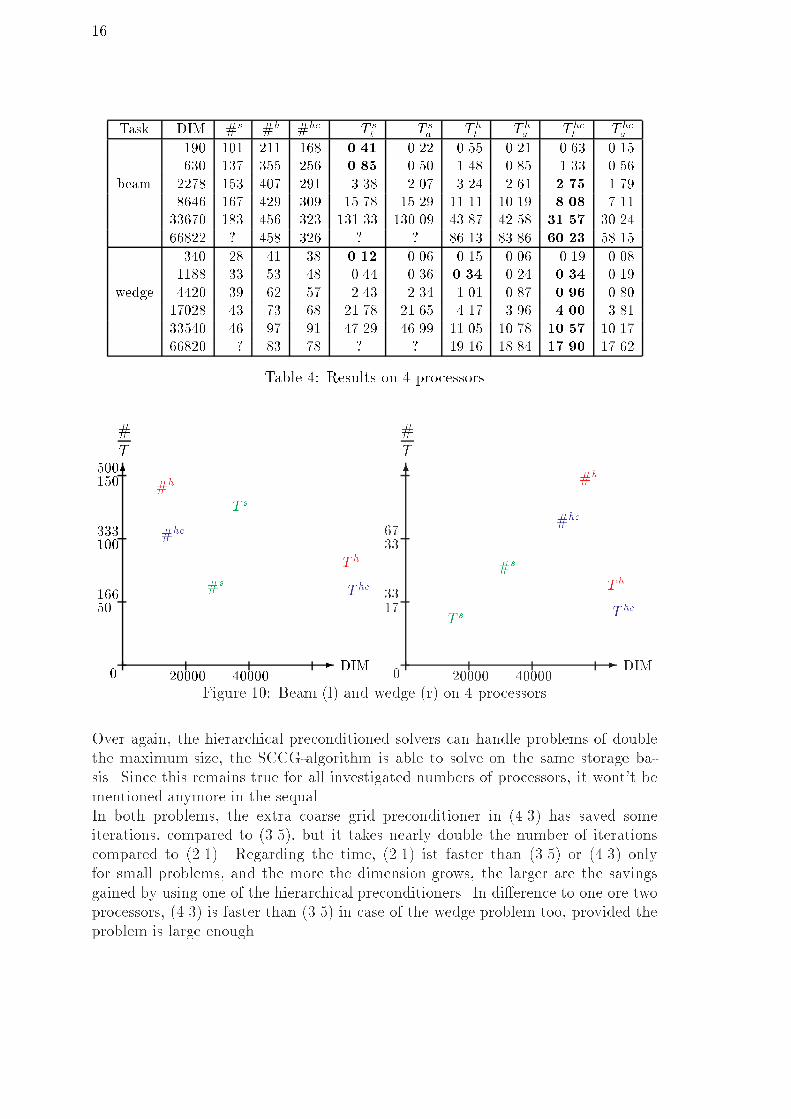
16 Task DIM #s #h #hc T st T sa Tht Tha Thct Thca190 101 211 168 0.41 0.22 0.55 0.21 0.63 0.15630 137 355 256 0.85 0.50 1.48 0.85 1.33 0.56beam 2278 153 407 291 3.38 2.07 3.24 2.61 2.75 1.798646 167 429 309 15.78 15.29 11.11 10.19 8.08 7.1133670 183 456 323 131.33 130.09 43.87 42.58 31.57 30.2466822 ? 458 326 ? ? 86.13 83.86 60.23 58.15340 28 41 38 0.12 0.06 0.15 0.06 0.19 0.081188 33 53 48 0.44 0.36 0.34 0.24 0.34 0.19wedge 4420 39 62 57 2.43 2.34 1.01 0.87 0.96 0.8017028 43 73 68 21.78 21.65 4.17 3.96 4.00 3.8133540 46 97 91 47.29 46.99 11.05 10.78 10.57 10.1766820 ? 83 78 ? ? 19.16 18.84 17.90 17.62Table 4: Results on 4 processorsDIM

#T0 20000 40000

50033316650100150-

6 #s.............................................................................................................................................................................T s.........................................................................................................................................................................................................................................................................................................

...........................................................#h........................................................................................................................................................................................................................................................................................................................................................................................Th......................................................................................................................................................................................................................................................................................................................................................................... ....................... ...............................#hc..................................................................................................................................................................................................................................................................................................................................................Thc.......................................................................................................................................................................................................................................................................................................................................................................................................... DIM

#T0 20000 4000017336733 -6 #s....................................................................................................................................................................T s..............................................................................................................................................................................................................................................................................

...................................................................................

..... #h..................................................................................................................................................................................................................................................................................................................................................................Th...............................................................................................................................................................................................................................................................................................................................................................................................#hc...........................................................................................................................................................................................................................................................................................................................................................Thc.............................................................................................................................................................................................................................................................................................................................................................................................Figure 10: Beam (l) and wedge (r) on 4 processorsOver again, the hierarchical preconditioned solvers can handle problems of doublethe maximum size, the SCCG-algorithm is able to solve on the same storage ba-sis. Since this remains true for all investigated numbers of processors, it wont't bementioned anymore in the sequal.In both problems, the extra coarse grid preconditioner in (4.3) has saved someiterations, compared to (3.5), but it takes nearly double the number of iterationscompared to (2.1). Regarding the time, (2.1) ist faster than (3.5) or (4.3) onlyfor small problems, and the more the dimension grows, the larger are the savingsgained by using one of the hierarchical preconditioners. In di�erence to one ore twoprocessors, (4.3) is faster than (3.5) in case of the wedge problem too, provided theproblem is large enough.

17Since #h�#hc is much smaller for the wedge than for the beam, the time savingsT h�T hc are wee for the wedge but perceptible for the beam.The tiny di�erences Tt � Ta show, that the losses in time caused by the di�erenttypes of global assembly don't play a signi�cant role on 4 processors.Note that the leftmost segments of the graph related to the number of iterationsfor the wedge problem in �gs. 10 and 8 doesn't indicate a falling tendency. In thiscases, the largest resolvable problem was on a mesh with Nx 6=Ny and casual thismesh was anomalous well suited for the solver. The same applies to �g. 12.Eight processorsTask DIM #s #h #hc T st T sa Tht Tha Thct Thca390 121 190 135 0.39 0.29 0.54 0.17 0.90 0.281278 143 220 152 0.70 0.43 0.90 0.43 1.12 0.37beam 4590 167 243 166 2.75 2.36 2.16 1.51 1.86 1.0017358 186 259 180 19.46 18.86 6.84 6.11 5.16 4.3467470 206 286 189 148.08 146.94 28.31 27.45 18.93 17.87133902 ? 283 187 ? ? 52.95 51.14 36.30 34.99380 35 40 36 0.19 0.05 0.18 0.02 0.22 0.031260 43 52 47 0.55 0.32 0.35 0.17 0.36 0.12wedge 4556 51 62 56 1.24 1.05 0.74 0.46 0.76 0.4617292 57 74 67 6.16 5.89 2.53 2.13 2.34 1.8867340 65 85 77 59.26 58.73 10.35 9.89 9.06 8.42133644 ? 102 93 ? ? 23.07 21.93 20.95 19.87Table 5: Results on 8 processorsDIM

#T0 40000 80000

30020010050100150-

6 #s...................................................................................................................................................................................T s..................................................................................................................................................................................................................................................................................................................................

............................................................... #h....................................................................................................................................................................................................................................................................................................................................T h.......................................................................................................................................................................................................................................................................................................................................................................................................#hc............................................................................................................................................................................................................................................................................................................................Thc.............................................................................................................................................................................................................................................................................................................................................................................................. DIM

#T0 40000 80000255010050 -6 #s...............................................................................................................................................................................T s..................................................................................................................................................................................................................................................................................

...................................................................................................................................................

................. #h...................................................................................................................................................................................................................................................................................................................................Th.................................................................................................................................................................................................................................................................................................................................................................................................................#hc..................................................................................................................................................................................................................................................................................................................................T hc.............................................................................................................................................................................................................................................................................................................................................................................................................Figure 11: Beam (l) and wedge (r) on 8 processors

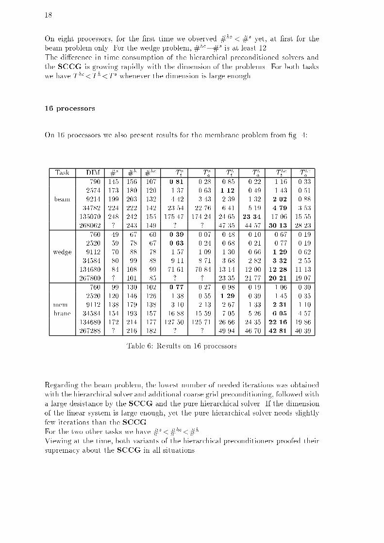
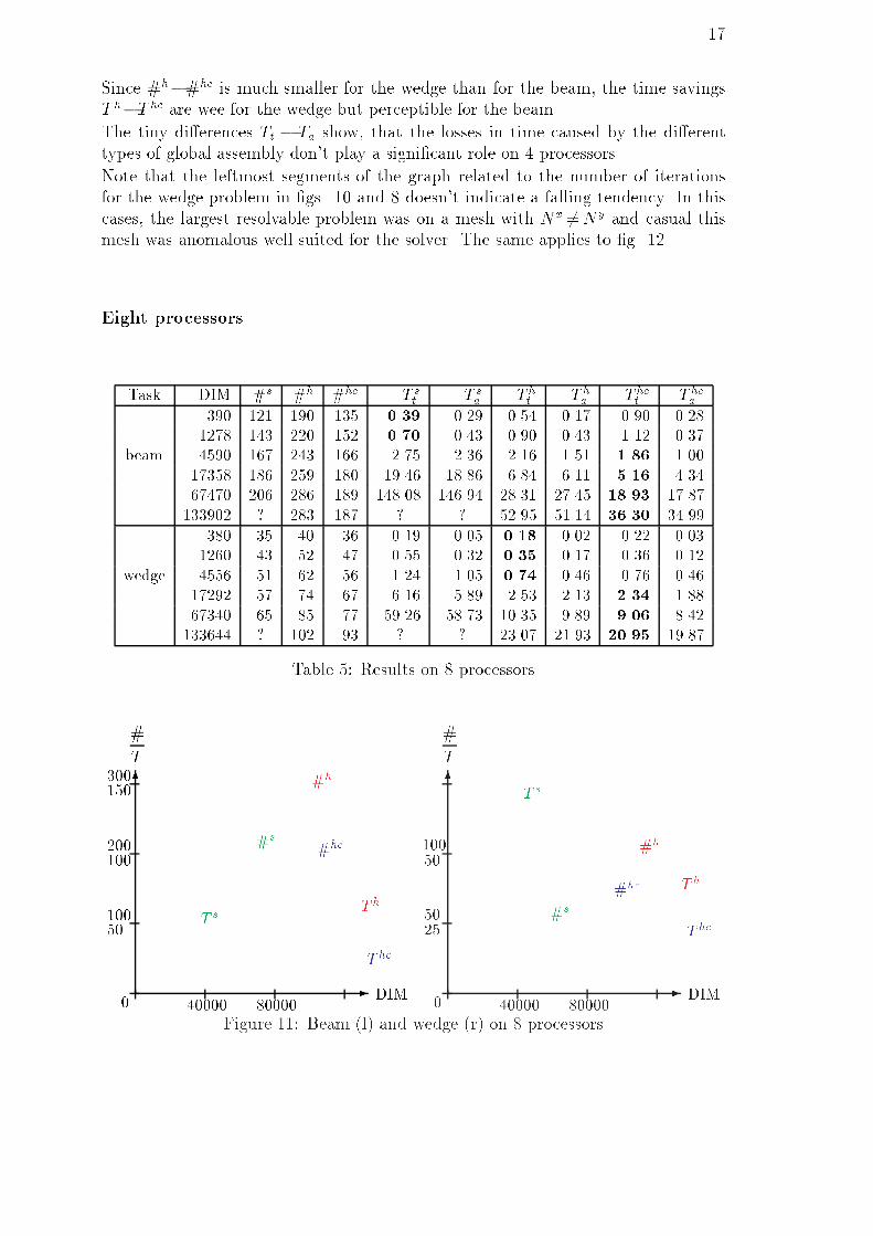
18On eight processors, for the �rst time we observed #hc < #s yet, at �rst for thebeam problem only. For the wedge problem, #hc�#s is at least 12.The di�erence in time consumption of the hierarchical preconditioned solvers andthe SCCG is growing rapidly with the dimension of the problems. For both taskswe have T hc<T h<T s whenever the dimension is large enough.16 processorsOn 16 processors we also present results for the membrane problem from �g. 4:Task DIM #s #h #hc T st T sa T ht Tha Thct Thca790 145 156 107 0.81 0.28 0.85 0.22 1.16 0.332574 173 180 120 1.37 0.63 1.12 0.49 1.43 0.51beam 9214 199 203 132 4.42 3.43 2.39 1.32 2.02 0.8834782 224 222 142 23.54 22.76 6.41 5.19 4.79 3.53135070 248 242 155 175.47 174.24 24.65 23.34 17.06 15.55268062 ? 243 149 ? ? 47.35 44.57 30.13 28.23760 49 67 60 0.39 0.07 0.48 0.10 0.67 0.192520 59 78 67 0.63 0.24 0.68 0.21 0.77 0.19wedge 9112 70 88 78 1.57 1.09 1.30 0.66 1.29 0.6234584 80 99 88 9.11 8.71 3.68 2.82 3.32 2.55134680 84 108 99 71.61 70.84 13.14 12.00 12.28 11.13267800 ? 101 85 ? ? 23.35 21.77 20.21 19.07760 99 130 102 0.77 0.27 0.98 0.19 1.06 0.302520 120 146 126 1.38 0.55 1.29 0.39 1.45 0.35mem{ 9112 138 179 138 3.10 2.13 2.67 1.33 2.31 1.10brane 34584 154 193 157 16.88 15.59 7.05 5.26 6.05 4.57134680 172 214 177 127.50 125.71 26.66 24.35 22.16 19.86267288 ? 216 182 ? ? 49.94 46.70 42.81 40.39Table 6: Results on 16 processorsRegarding the beam problem, the lowest number of needed iterations was obtainedwith the hierarchical solver and additional coarse grid preconditioning, followed witha large desistance by the SCCG and the pure hierarchical solver. If the dimensionof the linear system is large enough, yet the pure hierarchical solver needs slightlyfew iterations than the SCCG.For the two other tasks we have #s<#hc<#h.Viewing at the time, both variants of the hierarchical preconditioners proofed theirsupremacy about the SCCG in all situations.

19DIM

#T0 80000 16000020010050100150

-6 #s............................................................................................................................................................................................T s................................................................................................................................................................................................................................................................................

................................................................................................................................................

................ #h...............................................................................................................................................................................................................................................................................................................................Th....................................................................................................................................................................................................................................................................................................................................................................................................#hc............................................................................................................................................................................................................................................................................................................................T hc............................................................................................................................................................................................................................................................................................................................................................................................ DIM#T0 80000 160000255010050 -6 #s.................................................................................................................................................................................T s............................................................................................................................................................................................................................................................................................

.......................................................................................

..... #h................................................................................................................................................................................................................................................................................................................................Th....................................................................................................................................................................................................................................................................................................................................................................................................#hc.................................................................................................................................................................................................................................................................................................................................Thc...............................................................................................................................................................................................................................................................................................................................................................................................DIM

#T0 80000 16000020010050100 -6 #s.................................................................................................................................................................................T s............................................................................................................................................................................................................................................................................................................................................................. #h....................................................................................................................................................................................................................................................................................................................................Th.....................................................................................................................................................................................................................................................................................................................................................................................................#hc..............................................................................................................................................................................................................................................................................................................................T hc................................................................................................................................................................................................................................................................................................................................................................... ............................. Dotted lines = TaDrawn lines = TtFigure 12: Beam (ul), wedge (ur) and membrane (d) on 16 processors32 processorsTask DIM #s #h #hc T st T sa Tht Tha Thct Thca1590 234 200 103 1.49 0.37 1.05 0.23 1.47 0.305166 273 224 113 3.14 2.00 1.44 0.48 1.82 0.50beam 18462 308 245 122 8.32 7.00 2.91 1.54 2.43 1.0169630 344 264 134 35.45 33.66 7.67 6.49 5.12 3.43270270 377 283 144 259.63 253.27 29.89 27.21 16.60 13.98536382 ? 328 161 ? ? 65.01 61.72 34.42 30.251560 69 58 43 0.75 0.23 0.55 0.11 0.68 0.145112 81 68 53 1.19 0.59 0.73 0.18 0.98 0.34wedge 18360 91 78 62 2.44 1.86 1.39 0.59 1.49 0.6769432 101 90 72 11.81 10.87 3.63 2.56 3.41 2.08269880 109 102 82 87.47 86.06 13.44 11.43 11.47 9.48536120 ? 127 111 ? ? 31.77 29.07 28.49 25.15

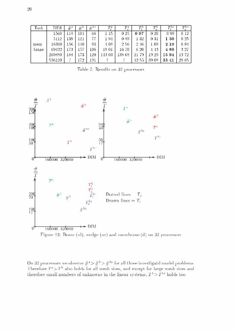
20 Task DIM #s #h #hc T st T sa Tht T ha Thct Thca1560 118 104 66 1.15 0.25 0.97 0.20 0.99 0.125112 139 121 77 1.94 0.89 1.32 0.31 1.30 0.25mem{ 18360 156 140 93 4.08 2.56 2.46 1.09 2.19 0.94brane 69432 173 157 106 18.01 16.70 6.20 4.43 4.80 3.27269880 188 173 120 143.03 138.68 21.79 19.29 15.94 13.72536120 ? 172 131 ? ? 42.55 39.08 33.41 29.85Table 7: Results on 32 processorsDIM

#T0 160000 320000

30020010050100150 -6 #s.....................................................................................................................................................................................................................T s...........................................................................................................................................................................................................................................................................................................................................................................

......................................................................... #h....................................................................................................................................................................................................................................................................................................................................T h...............................................................................................................................................................................................................................................................................................................................................................................................................#hc.............................................................................................................................................................................................................................................................................................................................T hc............................................................................................................................................................................................................................................................................................................................................................................................. DIM

#T0 160000 320000173310050 -6 #s...................................................................................................................................................................................T s....................................................................................................................................................................................................................................................................................................................

...........................................................................................

....... #h........................................................................................................................................................................................................................................................................................................................................T h........................................................................................................................................................................................................................................................................................................................................................................................................................................#hc........................................................................................................................................................................................................................................................................................................................................Thc..............................................................................................................................................................................................................................................................................................................................................................................................................................DIM

#T0 160000 3200002001001733 -6 #s.................................................................................................................................................................................T s.......................................................................................................................................................................................................................................................................................................

.....................................................................................................

........ #h..............................................................................................................................................................................................................................................................................................................................Tht.............................................................................................................................................................................................................................................................................................................................................................................................Tha..........................................................................#hc.............................................................................................................................................................................................................................................................................................................................T hct.....................................................................................................................................................................................................................................................................................................................................................................Thca.................................................................... Dotted lines = TaDrawn lines = TtFigure 13: Beam (ul), wedge (ur) and membrane (d) on 32 processorsOn 32 processors we observe #s>#h>#hc for all three investigatd model problems.Therefore T s>T h also holds for all mesh sizes, and except for large mesh sizes andtherefore small numbers of unknowns in the linear systems, T h>T hc holds too.

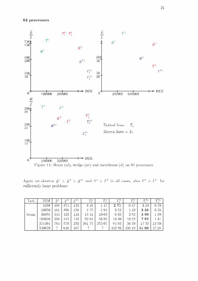
2164 processorsDIM

#T0 160000 320000

75050025050100150-

6 #s......................................................................................................................................................................................................T s................................................................................................................................................................................................................................................................

.........................................................................................................................

............. #h................................................................................................................................................................................................................................................................................................................................Tht.........................................................................................................................................................................................................................................................................................................................

................................................................................. T ha.................................................................

................. #hc............................................................................................................................................................................................................................................................................................................................................T hct...............................................................................................................................................................................................................................................................................................................................T hca.................. .............. .............................. DIM#T0 320000 640000204010050 -6 #s...........................................................................................................................................................................................................T s....................................................................................................................................................................................................................................................................

......................................................................................................................................

................ #h..............................................................................................................................................................................................................................................................................................................................................Th...............................................................................................................................................................................................................................................................................................................................................................................................................#hc.....................................................................................................................................................................................................................................................................................................................................Thc.............................................................................................................................................................................................................................................................................................................................................................................................................DIM

#T0 160000 320000

300200100122538 -6 #s...................................................................................................................................................................................................................................................................................................................................T s...........................................................................................................................................................................................................................................

................................................................................

....... #h............................................................................................................................................................................................................................................................................................................................Tht.....................................................................................................................................................................................................................................................................................................................................................................................................Tha..........................................................................

.#hc......................................................................................................................................................................................................................................................................................................................T hct................................................................................................................................................................................................................................................................................................................................................................Thca.................................................................... Dotted lines = TaDrawn lines = TtFigure 14: Beam (ul), wedge (ur) and membrane (d) on 64 processorsAgain we observe #s > #h > #hc and T s > T h in all cases, also T h > T hc forsu�ciently large problems.Task DIM #s #h #hc T st T sa Tht Tha Thct Thca3190 408 371 132 3.16 1.17 2.71 0.47 3.10 0.7010350 481 398 138 4.75 1.94 3.53 1.10 3.33 0.76beam 36958 544 422 143 13.41 10.03 6.02 2.82 3.99 1.39139326 598 445 159 59.94 56.98 13.30 10.82 7.92 4.31274494 764 570 233 261.75 255.07 84.92 56.29 17.32 12.50540670 ? 646 467 ? ? 442.86 438.19 51.60 47.28

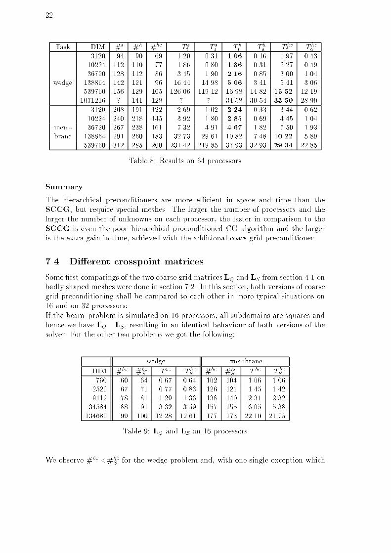
22 Task DIM #s #h #hc T st T sa Tht Tha Thct Thca3120 94 90 69 1.20 0.31 1.06 0.16 1.97 0.4310224 112 110 77 1.86 0.80 1.36 0.31 2.27 0.4936720 128 112 86 3.45 1.90 2.16 0.85 3.00 1.04wedge 138864 142 121 96 16.44 14.98 5.06 3.41 5.41 3.06539760 156 129 105 126.06 119.12 16.98 14.82 15.52 12.191071216 ? 141 128 ? ? 34.58 30.54 33.50 28.903120 208 191 122 2.69 1.02 2.24 0.33 3.44 0.6210224 240 218 145 3.92 1.80 2.85 0.69 4.45 1.04mem- 36720 267 238 161 7.32 4.91 4.67 1.82 5.50 1.93brane 138864 291 260 183 32.73 29.61 10.82 7.48 10.22 5.89539760 312 285 200 231.42 219.85 37.93 32.93 29.34 22.85Table 8: Results on 64 processorsSummaryThe hierarchical preconditioners are more e�cient in space and time than theSCCG, but require special meshes. The larger the number of processors and thelarger the number of unknowns on each processor, the faster in comparison to theSCCG is even the poor hierarchical proconditioned CG{algorithm and the largeris the extra gain in time, achieved with the additional coars grid preconditioner.7.4 Di�erent crosspoint matricesSome �rst comparings of the two coarse grid matrices LQ and LS from section 4.1 onbadly shaped meshes were done in section 7.2. In this section, both versions of coarsegrid preconditioning shall be compared to each other in more typical situations on16 and on 32 processors:If the beam{problem is simulated on 16 processors, all subdomains are squares andhence we have LQ=LS , resulting in an identical behaviour of both versions of thesolver. For the other two problems we got the following:wedge membraneDIM #hc #hcS Thc ThcS #hc #hcS Thc ThcS760 60 64 0.67 0.64 102 104 1.06 1.062520 67 71 0.77 0.83 126 121 1.45 1.429112 78 81 1.29 1.36 138 140 2.31 2.3234584 88 91 3.32 3.59 157 155 6.05 5.38134680 99 100 12.28 12.61 177 173 22.10 21.75Table 9: LQ and LS on 16 processorsWe observe #hc<#hcS for the wedge problem and, with one single exception which

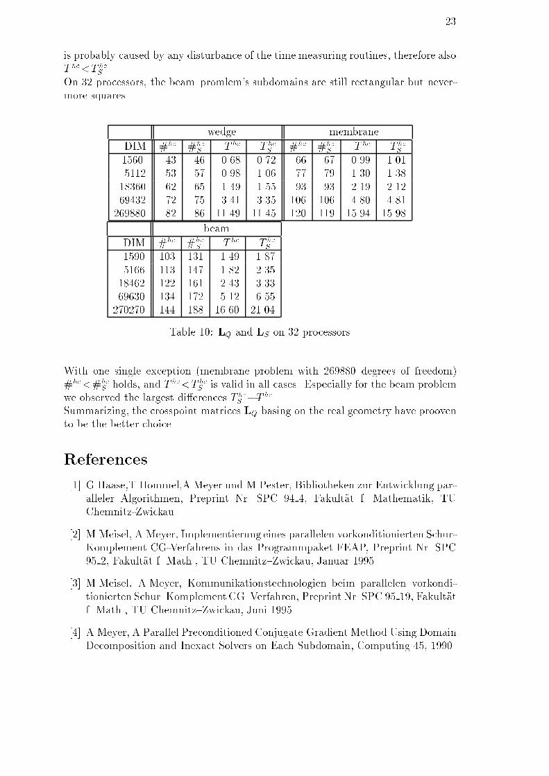
23is probably caused by any disturbance of the time measuring routines, therefore alsoT hc<T hcS .On 32 processors, the beam{promlem's subdomains are still rectangular but never-more squares. wedge membraneDIM #hc #hcS T hc T hcS #hc #hcS T hc T hcS1560 43 46 0.68 0.72 66 67 0.99 1.015112 53 57 0.98 1.06 77 79 1.30 1.3818360 62 65 1.49 1.55 93 93 2.19 2.1269432 72 75 3.41 3.35 106 106 4.80 4.81269880 82 86 11.49 11.45 120 119 15.94 15.98beamDIM #hc #hcS T hc T hcS1590 103 131 1.49 1.875166 113 147 1.82 2.3518462 122 161 2.43 3.3369630 134 172 5.12 6.55270270 144 188 16.60 21.04Table 10: LQ and LS on 32 processorsWith one single exception (membrane problem with 269880 degrees of freedom)#hc<#hcS holds, and T hc<T hcS is valid in all cases. Especially for the beam problemwe observed the largest di�erences T hcS �T hc.Summarizing, the crosspoint matrices LQ basing on the real geometry have proovento be the better choice.References[1] G.Haase,T.Hommel,A.Meyer und M.Pester, Bibliotheken zur Entwicklung par-alleler Algorithmen, Preprint Nr. SPC 94 4, Fakult�at f. Mathematik, TUChemnitz-Zwickau[2] M.Meisel, A.Meyer, Implementierung eines parallelen vorkonditionierten Schur-Komplement CG-Verfahrens in das Programmpaket FEAP, Preprint Nr. SPC95 2, Fakult�at f. Math., TU Chemnitz{Zwickau, Januar 1995[3] M.Meisel, A.Meyer, Kommunikationstechnologien beim parallelen vorkondi-tionierten Schur{KomplementCG{Verfahren, Preprint Nr. SPC 95 19, Fakult�atf. Math., TU Chemnitz{Zwickau, Juni 1995[4] A.Meyer, A Parallel Preconditioned Conjugate Gradient Method Using DomainDecomposition and Inexact Solvers on Each Subdomain, Computing 45, 1990.

[5] S.Meynen und P.Wriggers, T�atigkeitsbericht Darmstadt zum Forschungs-vorhaben Wr19/5-1 Parallele Iterationsverfahren, Technische Hochschule Darm-stadt, Institut f�ur Mechanik, Juli 1994[6] R.L.Taylor, FEAP - A finite element analysis program, Description and Users-Manual, University of California, Berkeley,1990[7] H.Yserentant, On the multilevel{splitting of �nite element spaces, Numer.Math. 49, 379{412 (1986)Other titles in the SFB393 series:96-01 V. Mehrmann, H. Xu. Chosing poles so that the single-input pole placement problemis well-conditioned. Januar 1996.96-02 T. Penzl. Numerical solution of generalized Lyapunov equations. January 1996.96-03 M. Scherzer, A. Meyer. Zur Berechnung von Spannungs- und Deformationsfeldernan Interface-Ecken im nichtlinearen Deformationsbereich auf Parallelrechnern.March 1996.96-04 Th. Frank, E. Wassen. Parallel solution algorithms for Lagrangian simulation ofdisperse multiphase ows. Proc. of 2nd Int. Symposium on Numerical Methods forMultiphase Flows, ASME Fluids Engineering Division Summer Meeting, July 7-11,1996, San Diego, CA, USA. June 1996.96-05 P. Benner, V. Mehrmann, H. Xu. A numerically stable, structure preserving methodfor computing the eigenvalues of real Hamiltonian or symplectic pencils. April 1996.96-06 P. Benner, R. Byers, E. Barth. HAMEV and SQRED: Fortran 77 Subroutinesfor Computing the Eigenvalues of Hamiltonian Matrices Using Van Loans's SquareReduced Method. May 1996.96-07 W. Rehm (Ed.). Portierbare numerische Simulation auf parallelen Architekturen.April 1996.96-08 J. Weickert. Navier-Stokes equations as a di�erential-algebraic system. August1996.96-09 R. Byers, C. He, V. Mehrmann. Where is the nearest non-regular pencil? August1996.96-10 Th. Apel. A note on anisotropic interpolation error estimates for isoparametricquadrilateral �nite elements. November 1996.96-11 Th. Apel, G. Lube. Anisotropic mesh re�nement for singularly perturbed reactiondi�usion problems. November 1996.

96-12 B. Heise, M. Jung. Scalability, e�ciency, and robustness of parallel multilevel solversfor nonlinear equations. September 1996.96-13 F. Milde, R. A. R�omer, M. Schreiber. Multifractal analysis of the metal-insulatortransition in anisotropic systems. October 1996.96-14 R. Schneider, P. L. Levin, M. Spasojevi�c. Multiscale compression of BEM equationsfor electrostatic systems. October 1996.96-15 M. Spasojevi�c, R. Schneider, P. L. Levin. On the creation of sparse BoundaryElement matrices for two dimensional electrostatics problems using the orthogonalHaar wavelet. October 1996.96-16 S. Dahlke, W. Dahmen, R. Hochmuth, R. Schneider. Stable multiscale bases andlocal error estimation for elliptic problems. October 1996.96-17 B. H. Kleemann, A. Rathsfeld, R. Schneider. Multiscale methods for BoundaryIntegral Equations and their application to boundary value problems in scatteringtheory and geodesy. October 1996.96-18 U. Reichel. Partitionierung von Finite-Elemente-Netzen. November 1996.96-19 W. Dahmen, R. Schneider. Composite wavelet bases for operator equations. Novem-ber 1996.96-20 R. A. R�omer, M. Schreiber. No enhancement of the localization length for twointeracting particles in a random potential. December 1996. to appear in: Phys.Rev. Lett., March 199796-21 G. Windisch. Two-point boundary value problems with piecewise constant coe�-cients: weak solution and exact discretization. December 1996.96-22 M. Jung, S. V. Nepomnyaschikh. Variable preconditioning procedures for ellipticproblems. December 1996.97-01 P. Benner, V. Mehrmann, H. Xu. A new method for computing the stable invariantsubspace of a real Hamiltonian matrix or Breaking Van Loan's curse? January 1997.97-02 B. Benhammouda. Rank-revealing 'top-down' ULV factorizations. January 1997.97-03 U. Schrader. Convergence of Asynchronous Jacobi-Newton-Iterations. January1997.97-04 U.-J. G�orke, R. Krei�ig. Ein u�faktoren bei der Identi�kation von Materialpa-rametern elastisch-plastischer Deformationsgesetze aus inhomogenen Verschiebungs-feldern. March 1997.97-05 U. Groh. FEM auf irregul�aren hierarchischen Dreiecksnetzen. March 1997.97-06 Th. Apel. Interpolation of non-smooth functions on anisotropic �nite elementmeshes. March 199797-07 Th. Apel, S. Nicaise. The �nite element method with anisotropic mesh grading forelliptic problems in domains with corners and edges.97-08 L. Grabowsky, Th. Ermer, J. Werner. Nutzung von MPI f�ur parallele FEM-Systeme. March 1997.97-09 T. Wappler, Th. Vojta, M. Schreiber. Monte-Carlo simulations of the dynamicalbehavior of the Coulomb glass. March 1997.

2697-10 M. Pester. Behandlung gekr�ummter Ober �achen in einem 3D-FEM-Programm f�urParallelrechner. April 1997.97-11 G. Globisch, S. V. Nepomnyaschikh. The hierarchical preconditioning having un-structured grids. April 1997.97-12 R. V. Pai, A. Punnoose, R. A. R�omer. The Mott-Anderson transition in the disor-dered one-dimensional Hubbard model. April 1997.97-13 M. Thess. Parallel Multilevel Preconditioners for Problems of Thin Smooth Shells.May 1997.97-14 A. Eilmes, R. A. R�omer, M. Schreiber. The two-dimensional Anderson model oflocalization with random hopping. June 1997.97-15 M. Jung, J. F. Maitre. Some remarks on the constant in the strengthened C.B.S.inequality: Application to h- and p-hierarchical �nite element discretizations ofelasticity problems. July 1997.97-16 G. Kunert. Error estimation for anisotropic tetrahedral and triangular �nite elementmeshes. August 1997.97-17 L. Grabowsky. MPI-basierte Koppelrandkommunikation und Ein u� der Partition-ierung im 3D-Fall. August 1997.97-18 R. A. R�omer, M. Schreiber. Weak delocalization dueto long-range interaction fortwo electrons in a random potential chain. August 1997.97-19 A. Eilmes, R. A. R�omer, M. Schreiber. Critical behavior in the two-dimensionalAnderson model of localization with random hopping. August 1997.The complete list of current and former preprints is available viahttp://www.tu-chemnitz.de/sfb393/sfb97pr.html.