a hybrid intelligent approach for metal-loss defect depth

A Hybrid Intelligent Approach forMetal-Loss Defect DepthPrediction in Oil and Gas Pipelines

Abduljalil Mohamed, Mohamed Salah Hamdi and Sofiène Tahar

Abstract The defect assessment process in oil and gas pipelines consists of threestages: defect detection, defect dimension (i.e., defect depth and length) prediction,anddefect severity level determination. In this paper,wepropose an intelligent systemapproach for defect prediction in oil and gas pipelines. The proposed techniqueis based on the magnetic flux leakage (MFL) technology widely used in pipelinemonitoring systems. In the first stage, theMFL signals are analyzed using theWavelettransform technique to detect anymetal-loss defect in the targeted pipeline. In case ofdefect existence, an adaptive neuro-fuzzy inference system is utilized to predict thedefect depth.Depth-related features are first extracted from theMFL signals, and thenused to train the neural network to tune the parameters of the membership functionsof the fuzzy inference system. To further improve the accuracy of the defect depth,predicted by the proposed model, highly-discriminant features are then selected byusing the weight-based support vector machine (SVM). Experimental work showsthat the proposed technique yields promising results, compared with those achievedby some service providers.

1 Introduction

It has been reported in [28] that the primary cause of approximately 30% of defectsin metallic long-distant pipelines, carrying crude oil and natural gas, is corrosion.To protect the surrounding environment from catastrophic consequences due to mal-functioning pipelines, an effective and efficient intelligent pipelinemonitoringsystem

A. Mohamed (B) · M.S. HamdiInformation Systems Department, Ahmed Bin Mohammed Military College, Doha, Qatare-mail: [email protected]

M.S. Hamdie-mail: [email protected]

S. TaharElectrical and Computer Engineering Department, Concordia University,Montreal, QC, Canadae-mail: [email protected]

© Springer International Publishing Switzerland 2016Y. Bi et al. (eds.), Intelligent Systems and Applications,Studies in Computational Intelligence 650, DOI 10.1007/978-3-319-33386-1_1

1

2 A. Mohamed et al.

is required. Non-destructive evaluation (NDE)-based monitoring tools, such asmagnetic sensors, are often employed to scan the pipelines [10, 29]. They are widelyused, on a regular basis, to measure any magnetic flux leakage (MFL) that mightbe caused by defects such as corrosion, cracks, dents, etc. It has been observed thatdefect characteristics (for example defect depth) can be predicted by examining theshape and amplitude of the obtained MFL signals [2, 11, 27]. Thus, the majorityof techniques reported in the literature rely heavily on the MFL signals. Other tech-niques that use other information sources such as ultrasonic waves and closed circuittelevision (CCTV) are also reported.

A reliability assessment of pipelines is a sequential process and consists mainlyof three stages: defect detection and classification [5, 17, 18, 33, 35, 38], defectdimension prediction [22–24, 35], and defect severity assessment [9, 14, 34]. At thefirst stage, a defect may be reported by an inline inspection tool, mechanical damageaccident, or visual examination. Then, the defect is associated to one of the possibledefect types such as gouges on welds, dents, cracking, corrosion, etc. In the nextstage, the dimensions (i.e., depth and length) of the identified defect are predicted.In the final stage, the defect severity level is determined. It is, based on the outcomeof this stage that an immediate response, such as pressure reductions or pipe repair,may be deemed urgent. The defect depth is an essential parameter in determining theseverity level of the detected defect. In [5], Artificial Neural Networks (ANNs) arefirst trained to distinguish defectedMFL signals from normalMFL signals. In case ofdefect existence,ANNsare applied to classify the defectMFLsignals into three defecttypes in the weld joint: external corrosion, internal corrosion, and lack of penetration.The proposed technique achieves a detection rate of 94.2% and a classificationaccuracy of 92.2%. The authors in [33] use image processing techniques to extractrepresentative features from images of cracked pipes. To account for variations ofvalues in these obtained features, a neuro-fuzzy inference system is trained suchthat the parameters of membership functions are tuned accordingly. A Radial BasisFunctionNeural Network (RBFNN) is trained to identify corrosion types in pipelinesin [38], where artificial corrosion types are deliberately introduced on the pipeline,and theMFL data are then collected. The proposed Immune RBFNN (IRBFNN) wasable to correctly locate the corrosion and determine its size. In [17], statistical andphysical features are extracted fromMFLsignals and fed into amulti-layer perceptronneural network to identify defected signals. The identified defected signal is presentedto a wavelet basis function neural network to generate a three-dimensional signalprofile displayed on a virtual reality environment. In [18] a Support Vector Machine(SVM) is used to reconstruct shape features of three different defect types andused fordefect classification and sizing. In [35], the authors propose a wavelet neural networkapproach for defect detection and classification in oil pipelines using MFL signals.In [22–24], artificial neural networks and neuro-fuzzy systems are used to estimatedefect depths. In [22], static, cascaded, and dynamic feedforward neural networksare used for defect depth estimation. In [23], a self-organizing neural network is usedas a visualization technique to identify appropriate features that are fed into differentnetwork architectures. In [24], a weight-based support vector machine is used toselect the most relevant features that are fed into a neuro-fuzzy inference system.

A Hybrid Intelligent Approach for Metal-Loss Defect Depth … 3

For reliability assessment of pipelines, a fuzzy-neural network system is proposed in[34]. Sensitive parameters, representing the actual conditions of defected pipelines,are extracted from MFL signals and used to train the hybrid intelligent system. Theintelligent system is then used to estimate the probability of failure of the defectedpipeline. The authors in [9] propose an artificial neural network approach for defectclassification using some defect-related factors including metal-loss, age, operatingpressure, pipeline diameter. In [14], to reduce the number of features used in thedefect assessment stage, several techniques are utilized including support vectormachine, regression, principal component analysis, and partial least squares.

The rest of the paper is organized as follows. In Sect. 2, we review the reliabilityassessment process in oil and gas pipelines. The proposed hybrid intelligent systemfor defect depth prediction is introduced in Sect. 3. In Sect. 4, the performance eval-uation of the proposed approach is described. We conclude with final remarks inSect. 5.

2 Reliability Assessment of Oil and Gas Pipelines

The main components of the reliability assessment process of pipelines are shownin Fig. 1. After detecting the presence of a pipeline defect, the pipeline reliabilityassessment system estimates the size of the defect (i.e. its length and depth), andbased on that, it predicts the severity of the defect and takes a measureable action torectify the situation. In the following we briefly describe each component.

2.1 Data Processing

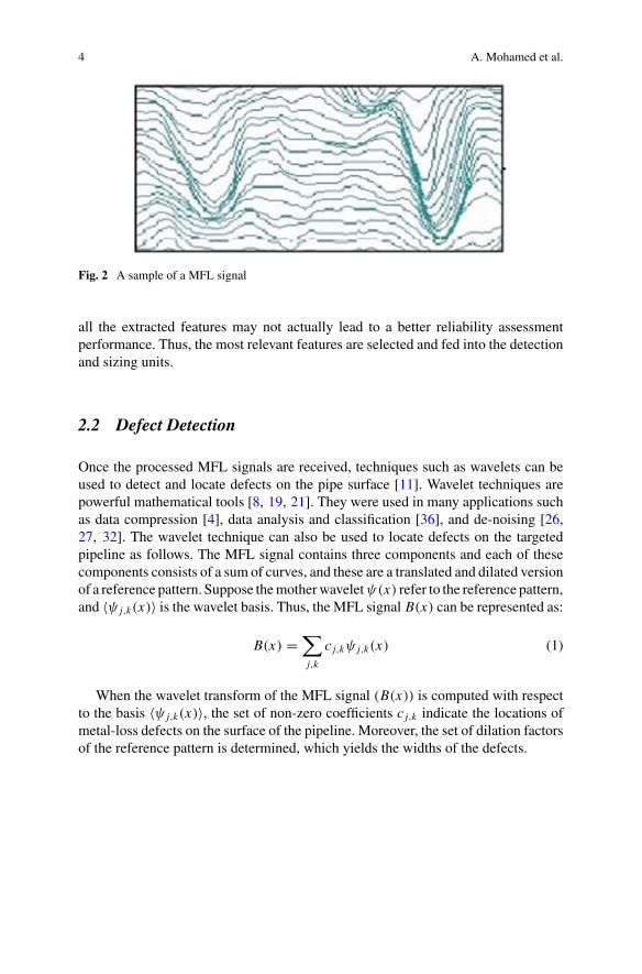
Nondestructive evaluation (NDE) tools are often used to scan pipelines for potentialdefects. One of theseNDE tools aremagnetic sensors that are attached to autonomousdevices sent periodically into the pipeline under inspection. The purpose of magneticsensors is to measure MFL signals [20], every 3mm along the pipeline length. Asample of a MFL signal is shown in Fig. 2. The amount of MFL data is huge, thusfeature extraction methods are needed to reduce data dimensionality. However, using

Fig. 1 Reliability assessment of pipelines

4 A. Mohamed et al.

Fig. 2 A sample of a MFL signal

all the extracted features may not actually lead to a better reliability assessmentperformance. Thus, the most relevant features are selected and fed into the detectionand sizing units.

2.2 Defect Detection

Once the processed MFL signals are received, techniques such as wavelets can beused to detect and locate defects on the pipe surface [11]. Wavelet techniques arepowerful mathematical tools [8, 19, 21]. They were used in many applications suchas data compression [4], data analysis and classification [36], and de-noising [26,27, 32]. The wavelet technique can also be used to locate defects on the targetedpipeline as follows. The MFL signal contains three components and each of thesecomponents consists of a sum of curves, and these are a translated and dilated versionof a reference pattern. Suppose themotherwaveletψ(x) refer to the reference pattern,and 〈ψ j,k(x)〉 is the wavelet basis. Thus, the MFL signal B(x) can be represented as:

B(x) =∑

j,k

c j,kψ j,k(x) (1)

When the wavelet transform of the MFL signal (B(x)) is computed with respectto the basis 〈ψ j,k(x)〉, the set of non-zero coefficients c j,k indicate the locations ofmetal-loss defects on the surface of the pipeline. Moreover, the set of dilation factorsof the reference pattern is determined, which yields the widths of the defects.


2.3 Defect Sizing

Defect sizing (in particular, determination of the defect depth) is an essential compo-nent of the reliability assessment system as, based on its outcome, the severity of thedetected defect can be determined. However, the relationship between the measuredMFL signals and the corresponding defect depth is not well-understood. Therefore,in the absence of feasible analytical models, hybrid intelligent tools such as AdaptiveNeuro-Fuzzy Inference systems (ANFIS) become indispensable and can be used tolearn this relationship [22–24, 35]. In this paper, after extracting and selecting mean-ingful features, an ANFIS model is trained using a hybrid learning algorithm thatcomprises least squares and the backpropagation gradient descent method [13].

2.4 Defect Assessment

Upon calculating the dimensions of the defect, its severity level can be determinedby using the industry standard [1]. Basic equations for assessing defects can be usedto construct defect acceptance curves as shown in Fig. 3 [7]. The first curve calcu-lates the failure stress of defects in the pipeline at the maximum operating pressure(MAOP), and the other curve shows the sizes of defects that would fail the hydropressure test [7].

2.5 Actions

The plot in Fig. 3 can be used to prioritize the repair of the defects. For example, twodefects are predicted to fail at the MAOP. For these defects, an immediate repair isneeded. Defects that have failure stresses lower than the hydro pressure curve areacceptable. Any defect between the assessing curves needs to be reassessed usingadvanced measuring tools.

3 A Hybrid Intelligent System for Defect Depth Estimation

The combination of neural networks and fuzzy inference systems has been success-fully used in different application areas such aswater qualitymanagement [31], queuemanagement [25], energy [37], transportation [15]; and business and manufacturing[6, 12, 16, 30]. In this section, the applicability of ANFIS models in estimatingmetal-loss defect depth is demonstrated. The general architecture of the proposedapproach is shown in Fig. 4.

6 A. Mohamed et al.

Fig. 3 Curves of defect assessment (Reproduced from [7])

Fig. 4 The structure diagram of the proposed approach

The proposed approach consists of three stages, namely: feature extraction, featureselection, and theANFISmodel. The three components are described in the followingsubsections.


Fig. 5 Features extracted for the radial component of the MFL signal

3.1 Feature Extraction

The main purpose of feature extraction is to reduce the MFL data dimensionality.As shown in Fig. 4, the MFL signal is represented by the axial, radial and tangentialcomponents. For each component, statistical and polynomial series are applied asfeature extraction methods. The features extracted from the radial component of theMFL signal are shown in Fig. 5. Statistical features are self-explanatory. Polynomialseries of the form an Xn + · · · + a1X + a0 can approximateMFL signals. Polynomi-als of degrees 3, 6, and 6 have been found to provide the best approximation for axial,radial, and tangential components, respectively. Thus, the input features consist ofthe polynomial coefficients, an, . . . , a0 along with the five statistical features. Thus,in total we have 33 features, which will be referred to by F1, F2,…, F33.

3.2 Feature Selection

It is a known fact that different features might exhibit different discrimination capa-bilities. Most often, incorporating all obtained features in the training process maynot lead to a high depth estimation accuracy. In fact, including some features mayhave a negative impact. Therefore, it is a common practice to identify the importantfeatures that are appropriate to the ANFSI model. Thus, the next step is to examinethe suitability of each feature for the defect depth prediction task. The best featuresthat yield the best depth estimation accuracy are then identified and used as an inputfeature pattern for the ANFIS model. Moreover, a support vector machine-basedweight correlation method is used to assign weights for the obtained features. Fea-tures with the highest weights are selected to train a new ANFIS model. Differentsets of features, having 16 to 29 features each, have been evaluated.

8 A. Mohamed et al.

Fig. 6 The architecture of ANFIS

3.3 The ANFIS Model

ANIFIS, as introduced by [13], is a hybrid neuro-fuzzy system, where the fuzzyIF-THEN rules and membership function parameters can be learned from trainingdata, instead of being obtained from an expert [3, 6, 12, 16, 25, 30, 31, 37].Whetherthe domain knowledge is available or not, the adaptive property of some of its nodesallows the network to generate the fuzzy rules that approximate a desired set ofinput-output pairs. In the following, we briefly introduce the ANFIS architecture asproposed in [13]. The structure of the ANFISmodel is basically a feedforward multi-layer network. The nodes in each layer are characterized by their specific function,and their outputs serve as inputs to the succeeding nodes. Only the parameters ofthe adaptive nodes (i.e., square nodes in Fig. 6) are adjustable during the trainingsession. Parameters of the other nodes (i.e., circle nodes in Fig. 6) are fixed.

Suppose there are two inputs x , y, and one output f . Let us also assume thatthe fuzzy rule in the fuzzy inference system is depicted by one degree of Sugeno’sfunction [13]. Thus, two fuzzy if-then rules will be contained in the rule base asfollows:

Rule 1: if x is A1 and y is B1 then f = p1x + q1y + r1.Rule 2: if x is A2 and y is B2 then f = p2x + q2y + r2.where pi , qi , ri are adaptable parameters.The node functions in each layer are described in the sequel.Layer 1: Each node in this layer is an adaptive node and is given as follows:

o1i = μAi (x), i = 1, 2 (2)

o1i = μBi−2(y), i = 3, 4 (3)


where x and y are inputs to the layer nodes, and Ai , Bi−2 are linguistic variables.The maximum and minimum of the bell-shaped membership function are 1 and 0,respectively. The membership function has the following form:

μAi (x) = 1

1 + {( x−ciai

)2}bi (4)

where the set {ai , bi , ci } represents the premise parameters of the membership func-tion. The bell-shaped function changes according to the change of values in theseparameters.

Layer 2: Each node in this layer is a fixed node. Its output is the product of thetwo input signals as follows:

o2i = wi = μAi (x)μBi (y), i = 1, 2 (5)

where wi refers to the firing strength of a rule.Layer 3: Each node in this layer is a fixed node. Its function is to normalize the

firing strength as follows:

o3i = w′′i = wi

w1 + w2, i = 1, 2 (6)

Layer 4: Each node in this layer is adaptive and adjusted as follows:

o4i = w′′i fi = w′′

i (pi x + qi y + ri ), i = 1, 2 (7)

where w′′i is the output of layer 3 and {pi + qi + ri } is the consequent parameter set.

Layer 5: Each node in this layer is fixed and computes its output as follows:

o5i =∑2

i=1w′′i fi = (

∑2i=1 wi fi )

w1 + w2(8)

The output of layer 5 sums the outputs of nodes in layer 4 to be the output ofthe whole network. If the parameters of the premise part are fixed, the output of thewhole network will be the linear combination of the consequent parameters, i.e.,

f = w1

w1 + w2f1 + w2

w1 + w2f2 (9)

The adopted training technique is hybrid, in which, the network node outputs goforward till layer 4, and the resulting parameters are identified by the least squaremethod. The error signal, however, goes backward till layer 1, and the premiseparameters are updated according to the descent gradient method. It has been shown

10 A. Mohamed et al.

in the literature that the hybrid-learning technique can obtain the optimal premiseand consequent parameters in the learning process [13].

3.4 Learning Algorithm for ANFIS

To map the input/output data set, the adaptable parameters {ai + bi + ci } and {pi +qi + ri } in theANFIS structure are adjusted in the learning process.When the premiseparameters ai , bi and ci of the membership function are fixed, the ANFIS yields thefollowing output as shown in (9). Substituting (6) into (9), we obtain the following:

f = w′′1 f1 + w′′

2 f2 (10)

Substituting the fuzzy if-then rules in (10) yields:

f = w′′1(p1x + q1y + r1) + w′′

2(p2x + q2y + r2) (11)

or:

f = (w′′1x)p1 + (w′′

1 y)q1 + (w′′1)r1) + (w′′

2x)p2 + (w′′2 y)q2 + (w′′

2)r2 (12)

Equation (12) is a linear combination of the adjustable parameters. The optimalvalues of {ai , bi , ci } and {pi , qi , ri } canbeobtainedbyusing the least squaredmethod.If the premise parameters are fixed, the hybrid learning algorithm can effectivelysearch for the optimal ANFIS parameters.

4 Experimental Results

To evaluate the effectiveness of the proposed technique, in terms of defect depthestimation accuracy, extensive experimental work has been carried out. The obtainedaccuracies are evaluated based on different levels of error-tolerance including: ±1,±5, ±10, ±15, ±20, ±25, ±30, ±35, and ±40%. The impact of using selectedfeatures, while utilizing different number and type of membership functions forthe adaptive nodes in the ANFIS model is studied. The results are reported in thefollowing subsections.

4.1 Types of Membership Functions for the Adaptive Nodes

The shape of the selected membership function (MF) defines how each point in theuniverse of discourse of the corresponding feature is mapped into a membership


value between 0 and 1 (the membership value indicates the degree to which therelevant input feature belongs to a certain metal-loss defect depth). The parametersthat control the shape of the membership function are tuned in the adaptive nodes,during the training session. The number of parameters needed depends on the typeof the membership function used in the adaptive node. Three types of membershipfunctions namely Gaussian, Trapezoidal, and Triangle for the feature F1 are shownin Fig. 7.

It can be seen from Fig. 7 that the smoothness of transition from one fuzzy set toanother varies, depending on the function type used in the adaptive node.

4.2 Training, Testing, and Validation Data

During the training session, four of the obtained features, namely F3, F6, F8, andF13, were not acceptable by theMatlabANFISmodel. Their sigma values were closeto zero so they were discarded. Thus, only 29 features of the 33 above mentionedfeatures were considered. The 1357 data samples, used for developing and testing theANFIS model, were divided as follows: 70% for training, 15% for testing, and 15%for validation (checking). The training data set consists of 949 rows and 30 columns.The rows represent the training samples, and the first 29 columns represent theextracted features of each sample and the last column represents the target (defectdepth). The format of the testing and validation data sets is similar to that of thetraining data set, however, each consists of 204 rows (samples). We have used 100epochs to train the ANFIS model.

A hybrid learning approach was adopted, in which the membership function para-meters of the single-out Sugeno type fuzzy inference system were identified. Thehybrid learning approach converges much faster than the original backpropagationmethod. In the forward pass, the node outputs go forward until layer 4 and the con-sequent parameters are identified with the least square method. In the backwardpass, the error rates propagate backwards and the premise parameters are updatedby gradient decent.

4.3 Evaluation of the Feature Prediction Power

In this section, the performance of each feature, in terms of its defect depth predictionaccuracy, is examined. Due to limited space, only the features that yield the bestprediction accuracy are reported. As shown in Table1, seven features present thebest estimation accuracy among all features, namely F1, F4, F9, F10, F11, F14, andF32. As expected, for the lower levels of error tolerance (particularly: ±10, ±15,and ±20%), none of the features yielded an acceptable prediction accuracy.


Fig. 7 Membership functions of the feature F1 a Gaussian, b trapezoidal, and c triangle

4.4 Using the Best Features

To improve the defect depth prediction accuracyof theANFISmodel, the features thatyield the best prediction accuracy are used to train the ANFISmodel. For 100 epochs,the training performance error of the ANFIS model is equal to 0.1482. The defectdepth prediction accuracy of this model is clearly improved as shown in Table2. Forerror-tolerance levels at ±10, ±15, and ±20%, the model gives prediction accuracyat 62, 74, and 87%, respectively.


Table 1 Defect depth prediction accuracy using the features F1, F4, F9, F10, F11, F14, and F32

Error-tolerance(%)

Input parameters

F1 F4 F9 F10 F11 F14 F32

±1 0.0196 0.0147 0.0294 0.0490 0.0196 0.0147 0.0392

±5 0.1176 0.1275 0.1618 0.1176 0.1373 0.1618 0.1275

±10 0.2892 0.2990 0.3627 0.2304 0.3235 0.2941 0.2941

±15 0.4510 0.4755 0.5637 0.4118 0.4902 0.5000 0.4608

±20 0.6275 0.6471 0.7549 0.5686 0.6667 0.6618 0.5882

±25 0.8137 0.8039 0.9265 0.6912 0.8137 0.8578 0.7010

±30 0.8775 0.8971 0.9461 0.7990 0.9020 0.9167 0.8480

±35 0.9265 0.9314 0.9510 0.9020 0.9412 0.9363 0.8922

±40 0.9461 0.9510 0.9559 0.9314 0.9559 0.9461 0.9265

Table 2 Defect depthprediction accuracy of theANFIS model using the bestfeatures

Error-tolerance (%) Input features (F1 F4 F9 F10F11 F14 F32)

±1 0.0637

±5 0.3529

±10 0.6127

±15 0.7402

±20 0.8725

±25 0.9314

±30 0.9510

±35 0.9755

±40 0.9853

4.5 Support Vector Machine-Based Feature Selection

Another method for evaluating the prediction power of the obtained features is byassigning a weight for each feature, based on the support vector machine weight-correlation technique. Features with the highest weights are selected to train theANFISmodel. After examining different sets of selected features, the first 22 featureshave yielded the best prediction accuracy as demonstrated in Table3.

As shown in Table3, for error-tolerance levels at±10,±15, and±20%, themodelgives a prediction accuracy at 62, 80, and 87%, respectively. It is slightly improvedover the best features, reported in Table2. For the error-tolerance level at ±10%, theprediction accuracy improved 1%, and for ±15%, improved 6%. However, for the±20% error-tolerance level, it remained the same as that of the best features. Only,using all the 29 features can give comparable results (shown in the last column ofTable3).


Table 3 Defect depth prediction accuracy of the ANFIS model using 22 features and all features

Error-tolerance (%) 22 Input features All features

±1 0.0637 0.0588

±5 0.3529 0.3627

±10 0.6225 0.6324

±15 0.8039 0.7990

±20 0.8775 0.8529

±25 0.9118 0.8971

±30 0.9559 0.9314

±35 0.9706 0.9510

±40 0.9804 0.9608

4.6 Using Different Membership Function Types

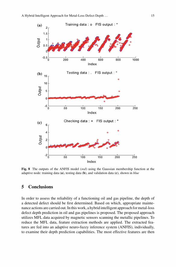
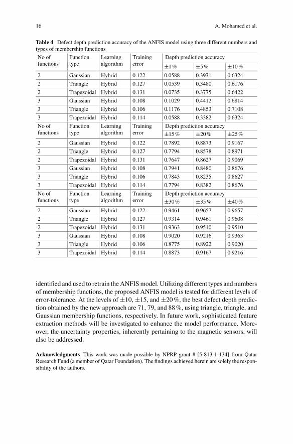
In this section, we examine the impact of using three different membership functiontypes on the model performance. In the model adaptive nodes, to each of the sevenbest features (i.e., F1, F4, F9, F10, F11, F14, and F32), we assigned Gaussian,trapezoidal, and triangle membership functions. The shapes of these functions areshown in Fig. 7. The number of membership functions is set at 2 or 3, for eachtype. The outputs of the ANFIS model for the training, testing and validation data(for Gaussian membership function) are shown in Fig. 8. The x-axis represents theindices of the training data elements, whereas the y-axis represents the defect depthsof the corresponding data elements. The 949 training data samples, representing thetrue defect depths, are plotted in blue (Fig. 8a).While themodel out puts, representingthe same defect depths estimated by the model, are plotted in red (Fig. 8a). Clearly,the model outputs (estimated defect depths) are satisfactory as they lie on or close tothe true defect depths. Figure8b, c show the model outputs (plotted in red) againstthe 204-element testing data (plotted in blue) and 204-element validation (checking)data (plotted in blue), respectively. The defect depth prediction accuracy, obtained bythe ANFIS model for the three types of membership functions, is shown in Table4,where the best accuracies are highlighted in red.

The model shows improvement for the error-tolerance levels ±1, ±5, and ±10%as it yield 11, 48, and 71%, respectively, compared to 6, 35, and 62% produced bythe ANFIS model using the 22 features. For the rest of the error-tolerance levels, ityields accuracies comparable to those produced by the ANFIS model using the 22features. The best training error is calculated at 0.106, obtained by the ANFIS modelusing three triangle membership functions.


Fig. 8 The outputs of the ANFIS model (red) using the Gaussian membership function at theadaptive node: training data (a), testing data (b), and validation data (c), shown in blue

5 Conclusions

In order to assess the reliability of a functioning oil and gas pipeline, the depth ofa detected defect should be first determined. Based on which, appropriate mainte-nance actions are carried out. In thiswork, a hybrid intelligent approach formetal-lossdefect depth prediction in oil and gas pipelines is proposed. The proposed approachutilizes MFL data acquired by magnetic sensors scanning the metallic pipelines. Toreduce the MFL data, feature extraction methods are applied. The extracted fea-tures are fed into an adaptive neuro-fuzzy inference system (ANFIS), individually,to examine their depth prediction capabilities. The most effective features are then


Table 4 Defect depth prediction accuracy of the ANFIS model using three different numbers andtypes of membership functions

No offunctions

Functiontype

Learningalgorithm

Trainingerror

Depth prediction accuracy

±1% ±5% ±10%

2 Gaussian Hybrid 0.122 0.0588 0.3971 0.6324

2 Triangle Hybrid 0.127 0.0539 0.3480 0.6176

2 Trapezoidal Hybrid 0.131 0.0735 0.3775 0.6422

3 Gaussian Hybrid 0.108 0.1029 0.4412 0.6814

3 Triangle Hybrid 0.106 0.1176 0.4853 0.7108


No offunctions

Functiontype

Learningalgorithm

Trainingerror


±15% ±20% ±25%

2 Gaussian Hybrid 0.122 0.7892 0.8873 0.9167

2 Triangle Hybrid 0.127 0.7794 0.8578 0.8971


3 Gaussian Hybrid 0.108 0.7941 0.8480 0.8676

3 Triangle Hybrid 0.106 0.7843 0.8235 0.8627


No offunctions

Functiontype

Learningalgorithm

Trainingerror


±30% ±35% ±40%

2 Gaussian Hybrid 0.122 0.9461 0.9657 0.9657

2 Triangle Hybrid 0.127 0.9314 0.9461 0.9608


3 Gaussian Hybrid 0.108 0.9020 0.9216 0.9363

3 Triangle Hybrid 0.106 0.8775 0.8922 0.9020


identified and used to retrain theANFISmodel. Utilizing different types and numbersof membership functions, the proposed ANFIS model is tested for different levels oferror-tolerance. At the levels of ±10, ±15, and ±20%, the best defect depth predic-tion obtained by the new approach are 71, 79, and 88%, using triangle, triangle, andGaussian membership functions, respectively. In future work, sophisticated featureextraction methods will be investigated to enhance the model performance. More-over, the uncertainty properties, inherently pertaining to the magnetic sensors, willalso be addressed.

Acknowledgments This work was made possible by NPRP grant # [5-813-1-134] from QatarResearch Fund (a member of Qatar Foundation). The findings achieved herein are solely the respon-sibility of the authors.


References

1. American Society ofMechanical Engineers: ASMEB31GManual for Determining RemainingStrength of Corroded Pipelines (1991)

2. Amineh, R., et al.: A space mapping methodology for defect characterization from magneticflux leakage measurement. IEEE Trans. Magn. 44(8), 2058–2065 (2008)

3. Azamathulla, H., Ab Ghani, A., Yen Fei, S.: ANFIS-based approach for predicting sedimenttransport in clean sewer. Appl. Soft Comput. 12(3), 1227–1230 (2012)

4. Bradley, J., Bradley, C., Brislawn, C., Hopper, T.: FBI wavelet/scalar quantization standard forgray-scale fingerprint image compression. SPIE Proc., Visual Inf. Process. II 1961, 293–304(1993)

5. Carvalho, A., et al.: MFL signals and artificial neural network applied to detection and classi-fication of pipe weld defects. NDT Int. 39(8), 661–667 (2006)

6. Chen, M.: A hybrid ANFIS model for business failure prediction utilizing particle swarmoptimization and subtractive clustering. Inf. Sci. 220, 180–195 (2013)

7. Cosham, A., Kirkwood, M.: Best practice in pipeline defect assessment. Paper IPC00-0205,International Pipeline Conference (2000)

8. Daubechies, I.: Ten Lectures on Wavelets. SIAM: Society for Industrial and Applied Mathe-matics, Philadelphia (1992)

9. El-Abbasy, M., et al.: Artificial neural network models for predicting condition of offshore oiland gas pipelines. Autom. Constr. 45, 50–65 (2014)

10. Gloria, N., et al.: Development of a magnetic sensor for detection and sizing of internal pipelinecorrosion defects. NDT E Int. 42(8), 669–677 (2009)

11. Hwang, K., et al.: Characterization of gas pipeline inspection signals using wavelet basisfunction neural networks. NDT E Int. 33(8), 531–545 (2000)

12. Iphar, M.: ANN and ANFIS performance prediction models for hydraulic impact hammers.Tunn. Undergr. Space Technol. 27(1), 23–29 (2012)

13. Jang, J.: ANFIS: adaptive-network-based fuzzy inference system. IEEE Trans. Syst., MAN,Cybern. 23, 665–685 (1993)

14. Khodayari-Rostamabad, A., et al.: Machine learning techniques for the analysis of magneticflux leakage images in pipeline inspection. IEEE Trans. Magn. 45(8), 3073–3084 (2009)

15. Khodayari, A., et al.: ANFIS based modeling and prediction car following behavior in realtraffic flow based on instantaneous reaction delay. In: IEEE Intelligent Transportation SystemsConference, pp. 599–604 (2012)

16. Kulaksiz, A.: ANFIS-based estimation of PV module equivalent parameters: application toa stand-alone PV system with MPPT controller. Turk. J. Electr. Eng. Comput. Sci. 21(2),2127–2140 (2013)

17. Lee, J., et al.: Hierarchical rule based classification of MFL signals obtained from natural gaspipeline inspection. In: International Joint Conference on Neural Networks, vol. 5 (2000)

18. Lijian, Y., et al.: Oil-gas pipeline magnetic flux leakage testing defect reconstruction basedon support vector machine. In: Second International Conference on Intelligent ComputationTechnology and Automation, vol. 2 (2009)

19. Mallat, S.: A Wavelet Tour of Signal Processing. Academic, New York (2008)20. Mandal, K., Atherton, D.: A study of magnetic flux-leakage signals. J. Phys. D: Appl. Phys.

31(22), 3211 (1998)21. Misiti, M., Misiti, Y., Oppenheim, G., Poggi, J.: Wavelets and Their Applications.Wiley-ISTE,

New York (2007)22. Mohamed, A., Hamdi, M.S., Tahar, S.: A machine learning approach for big data in oil and

gas pipelines. In: 3rd International Conference on Future Internet of Things and Cloud (2015)23. Mohamed, A., Hamdi, M.S., Tahar, S.: Self-organizing map-based feature visualization and

selection for defect depth estimation in oil and gas pipelines. In: 19th International Conferenceon Information Visualization (2015)


24. Mohamed, A., Hamdi, M.S., Tahar, S.: An adaptive neuro-fuzzy inference system-basedapproach for oil and gas pipeline defect depth estimation. In: SAI Intelligent Systems Confer-ence (2015)

25. Mucsi, K., Ata, K., Mojtaba, A.: An adaptive neuro-fuzzy inference system for estimating thenumber of vehicles for queue management at signalized intersections. Transp. Res. Part C:Emerg. Technol. 19(6), 1033–1047 (2011)

26. Muhammad, A., Udpa, S.: Advanced signal processing of magnetic flux leakage data obtainedfrom seamless gas pipeline. NDT E Int. 35(7), 449–457 (2002)

27. Mukhopadhyay, S., Srivastave,G.:Characterization ofmetal-loss defects frommagnetic signalswith discrete wavelet transform. NDT Int. 33(1), 57–65 (2000)

28. Nicholson, P.: Combined CIPS and DCVG survey for more accurate ECDS data. J. WorldPipelines 7, 1–7 (2007)

29. Park, G., Park, E.: Improvement of the sensor system in magnetic flux leakage-type nod-destructive testing. IEEE Trans. Magn. 38(2), 1277–1280 (2002)

30. Petkovic, D., et al.: Adaptive neuro-fuzzy estimation of conductive silicone rubber mechanicalproperties. Expert Syst. Appl. 39(10), 9477–9482 (2012)

31. Roohollah, N., Safavi, S., Shahrokni, S.: A reduced-order adaptive neuro-fuzzy inference sys-tem model as a software sensor for rapid estimation of five-day biochemical oxygen demand.J. Hydrol. 495, 175–185 (2013)

32. Shou-peng, S., Pei-wen, Q.: Wavelet based noise suppression technique and its application toultrasonic flaw detection. Ultrasonics 44(2), 188–193 (2006)

33. Sinha, S.,Karray, F.:Classificationof undergroundpipe scanned images using feature extractionand neuro-fuzzy algorithm. IEEE Trans. Neural Netw. 13(2), 393–401 (2002)

34. Sinha, S., Pandey, M.: Probabilistic neural network for reliability assessment of oil and gaspipelines. Comput.-Aided Civil Infrastruct. Eng. 17(5), 320–329 (2002)

35. Tikaria, M., Nema, S.: Wavelet neural network based intelligent system for oil pipeline defectcharacterization. In: 3rd International Conference on Emerging Trends in Engineering andTechnology (ICETET) (2010)

36. Unser, M., Aldroubi, A.: A review of wavelets in biomedical applications. Proc. IEEE 84(4),626–638 (1996)

37. Zadeh, A., et al.: An emotional learning-neuro-fuzzy inference approach for optimum trainingand forecasting of gas consumption estimation models with cognitive data. Technol. Forecast.Soc. Change 91, 47–63 (2015)

38. Zhongli, M., Liu, H.: Pipeline defect detection and sizing based on MFL data using immuneRBF neural networks. In: IEEE Congress on Evolutionary Computation pp. 3399–3403 (2007)

a hybrid intelligent approach for metal-loss defect depth

Documents