a life-cycle methodology for energy use by in-place

CIVIL ENGINEERING STUDIES

Illinois Center for Transportation Series No. 20-018 UILU-ENG-2020-2018

ISSN: 0197-9191

A Life-Cycle Methodology for Energy Use

by In-Place Pavement Recycling Techniques

Prepared By Imad L. Al-Qadi

Hasan Ozer Mouna Krami Senhaji

Qingwen Zhou Rebekah Yang Seunggu Kang

Marshall Thompson John Harvey

Arash Saboori Ali Butt

Hao Wang Xiaodan Chen

Research Report No. ICT-20-2018

A report of the findings of

A Life-Cycle Methodology for Energy Use by In-Place Pavement Recycling Techniques

https://doi.org/10.36501/0197-9191/20-018

Illinois Center for Transportation

October 2020

TECHNICAL REPORT DOCUMENTATION PAGE

1. Report No. ICT-20-018

2. Government Accession No.

N/A

3. Recipient’s Catalog No.

N/A

4. Title and Subtitle

A Life-Cycle Methodology for Energy Use by In-Place Pavement Recycling Techniques

5. Report Date

October 2020

6. Performing Organization Code

N/A

7. Authors

Imad L. Al-Qadi, Hasan Ozer, Mouna Krami Senhaji, Qingwen Zhou, Rebekah Yang, Seunggu Kang, Marshall Thompson, John Harvey, Arash Saboori, Ali Butt, Hao Wang, Xiaodan Chen

8. Performing Organization Report No.

ICT-20-018

UILU-ENG-2020-2018

9. Performing Organization Name and Address

Illinois Center for Transportation

Department of Civil and Environmental Engineering

University of Illinois at Urbana-Champaign

205 North Mathews Avenue, MC-250

Urbana, IL 61801

10. Work Unit No.

N/A

11. Contract or Grant No.

DTFH6114C00046

12. Sponsoring Agency Name and Address

Office of Research, Development, and Technology

Federal Highway Administration

6300 Georgetown Pike

McLean, VA 22101-2296

13. Type of Report and Period Covered

Final Report 9/15–9/17

14. Sponsoring Agency Code

15. Supplementary Notes

https://doi.org/10.36501/0197-9191/20-018

16. Abstract Worldwide interest in using recycled materials in flexible pavements as an alternative to virgin materials has increased

significantly over the past few decades. Therefore, recycling has been utilized in pavement maintenance and rehabilitation

activities. Three types of in-place recycling technologies have been introduced since the late 70s: hot in-place recycling, cold in-

place recycling, and full-depth reclamation. The main objectives of this project are to develop a framework and a life-cycle

assessment (LCA) methodology to evaluate maintenance and rehabilitation treatments, specifically in-place recycling and

conventional paving methods, and develop a LCA tool utilizing Visual Basic for Applications (VBA) to help local and state highway

agencies evaluate environmental benefits and tradeoffs of in-place recycling techniques as compared to conventional

rehabilitation methods at each life-cycle stage from the material extraction to the end of life. The ultimate outcome of this study

is the development of a framework and a user-friendly LCA tool that assesses the environmental impact of a wide range of

pavement treatments, including in-place recycling, conventional methods, and surface treatments. The developed tool provides

pavement industry practitioners, consultants, and agencies the opportunity to complement their projects’ economic and social

assessment with the environmental impacts quantification. In addition, the tool presents the main factors that impact produced

emissions and energy consumed at every stage of the pavement life cycle due to treatments. The tool provides detailed

information such as fuel usage analysis of in-place recycling based on field data.

17. Key Words

In-Place Recycling, Life-Cycle Assessment, Energy, Emission, Pavements, Rehabilitation

18. Distribution Statement

No restrictions. This document is available through the National Technical Information Service, Springfield, VA 22161.

19. Security Classif. (of this report) Unclassified

20. Security Classif. (of this page)

Unclassified

21. No. of Pages

128 + appendices

22. Price

N/A

Form DOT F 1700.7 (8-72) Reproduction of completed page authorized

i

ACKNOWLEDGMENT, DISCLAIMER, MANUFACTURERS’ NAMES

This publication is based on the results of ICT-20-018: A Life-Cycle Methodology for Energy Use by In-Place Pavement Recycling Techniques. ICT-R20-018 was conducted in cooperation with the Illinois Center for Transportation. The contents of this report reflect the view of the authors, who are responsible for the facts and the accuracy of the data presented herein. The contents do not necessarily reflect the official views or policies of the Illinois Center for Transportation. This report does not constitute a standard, specification, or regulation.

ii

EXECUTIVE SUMMARY

Worldwide interest in using recycled materials in flexible pavements as an alternative to virgin materials has increased significantly over the past few decades. Therefore, recycling has been utilized in pavement maintenance and rehabilitation activities. Three types of in-place recycling technologies have been introduced since the late 70s: hot in-place recycling, cold in-place recycling, and full-depth reclamation. They have been evolving through the use of new equipment trains, mix design specifications, and use of additives (e.g., engineered emulsion, lime, and cement). The advantages of using these evolving techniques include conservation of virgin materials, reduction of energy use and environmental impacts, reduction of construction time and traffic flow disruptions, reduction of number of hauling trucks, and improvement of pavement condition. The main objectives of this project are to develop a framework and a life-cycle assessment (LCA) methodology to evaluate maintenance and rehabilitation treatments, specifically in-place recycling and conventional paving methods; provide a fuel usage analysis of in-place recycling techniques during the construction stage; develop deterministic pavement performance models for in-place recycling techniques to predict pavement performance during the analysis period; and develop a LCA tool utilizing Visual Basic for Applications (VBA) to help local and state highway agencies to evaluate environmental benefits and tradeoffs of in-place recycling techniques as compared to conventional rehabilitation methods at each life-cycle stage from material extraction and production to the end of life. The ultimate outcome of this study is the development of a framework and a user-friendly LCA tool that assesses the environmental impact of a wide range of pavement treatments, including in-place recycling, conventional methods, and surface treatments. The tool utilizes data, simulation, and models through all in-place recycling stages for pavement LCA, including materials, construction, maintenance/rehabilitation, use, and end of life. The developed tool provides pavement industry practitioners, consultants, and agencies with the opportunity to complement their projects’ economic and social assessment with the environmental impacts of quantification. In addition, the tool presents the main factors that impact produced emissions and energy consumed at every stage of the pavement life cycle due to pavement treatment. The tool provides detailed information such as fuel usage analysis of in-place recycling techniques based on field data. It shows that fuel usage is affected by pavement hardness, pavement width, air temperature, and horsepower of the equipment used.

iii

TABLE OF CONTENTS

CHAPTER 1: INTRODUCTION ................................................................................................... 1

MOTIVATION ................................................................................................................................ 1

OBJECTIVES .................................................................................................................................. 3

METHODOLOGY ........................................................................................................................... 3

REPORT CONTENTS AND ORGANIZATION .................................................................................... 4

CHAPTER 2: REVIEW OF IN-PLACE RECYCLING TECHNIQUES ................................................... 6

IN-PLACE RECYCLING TECHNIQUES .............................................................................................. 6

Hot In-Place Recycling ............................................................................................................. 6

Cold In-Place Recycling ............................................................................................................ 8

Full-Depth Reclamation ......................................................................................................... 12

CHAPTER 3: GOAL AND SCOPE SUMMARY ............................................................................ 17

GOAL OF THE STUDY .................................................................................................................. 17

SCOPE OF THE STUDY ................................................................................................................. 17

Functional Unit ...................................................................................................................... 17

System Boundary ................................................................................................................... 17

Analysis Period ...................................................................................................................... 17

Allocation Method ................................................................................................................. 18

INVENTORY ANALYSIS AND IMPACT CATEGORIZATION ............................................................. 18

Global Warming Potential...................................................................................................... 19

Single Score ........................................................................................................................... 19

Energy Indicators ................................................................................................................... 19

CHAPTER 4: LIFE-CYCLE INVENTORY ANALYSIS ..................................................................... 20

DATA COLLECTION ..................................................................................................................... 20

Primary Data ......................................................................................................................... 20

Fuel Usage Models for IPR Techniques .................................................................................. 21

Secondary Data ..................................................................................................................... 32

Other Data Collected from Questionnaires (States) ............................................................... 32

MODELING PROCEDURES ........................................................................................................... 33

iv

Major Unit Process Modeled and Included in the Database ................................................... 33

ALLOCATION PROCEDURES ........................................................................................................ 43

Cut-Off Method ..................................................................................................................... 44

Substitution (Closed-loop Approximation) ............................................................................. 45

DATA QUALITY ASSESSMENT ..................................................................................................... 45

Data Quality Requirements.................................................................................................... 45

Data Validation ...................................................................................................................... 46

CHAPTER 5: PAVEMENT PERFORMANCE MODELING ............................................................ 48

OVERVIEW OF METHODS ........................................................................................................... 48

MULTI-CRITERIA PERFORMANCE ESTIMATION APPROACH ....................................................... 50

Concept ................................................................................................................................. 50

Development of Performance Estimation .............................................................................. 51

DETERMINISTIC PERFORMANCE MODELS .................................................................................. 57

Introduction .......................................................................................................................... 57

Data Collection ...................................................................................................................... 59

Performance Modeling .......................................................................................................... 63

CHAPTER 6: PAVEMENT USE STAGE ...................................................................................... 74

INTRODUCTION .......................................................................................................................... 74

MODELING APPROACH USED FOR USE STAGE EMISSIONS DUE TO ROUGHNESS ...................... 75

HDM-4 ................................................................................................................................... 76

Modeling Engine Using MOVES.............................................................................................. 78

Updating the Rolling Resistance Term ................................................................................... 80

Impact of Roughness on Rolling Resistance Modeling ............................................................ 81

TEXTURE-RELATED ROLLING RESISTANCE .................................................................................. 82

MAINTENANCE AND REHABILITATION SCHEDULE ..................................................................... 83

WORK ZONE MODELING ............................................................................................................ 83

CHAPTER 7: ANALYSIS AND INTERPRETATION ...................................................................... 85

SENSITIVITY ANALYSIS ................................................................................................................ 85

Analysis Period ...................................................................................................................... 85

End of Life ............................................................................................................................. 86

v

MAJOR ASSUMPTIONS AND LIMITATIONS ................................................................................. 93

CHAPTER 8: TOOL DEVELOPMENT......................................................................................... 94

PROGRAMMING PLATFORM ...................................................................................................... 94

MODULES ................................................................................................................................... 95

General Inputs ....................................................................................................................... 96

Treatment Selection .............................................................................................................. 97

Pavement Performance ......................................................................................................... 99

Materials Extraction and Production Stage .......................................................................... 103

Construction Stage .............................................................................................................. 105

Maintenance and Rehabilitation Stage ................................................................................ 107

Use Stage ............................................................................................................................ 109

End-of-Life Stage ................................................................................................................. 109

Review and Results .............................................................................................................. 109

CALCULATIONS ......................................................................................................................... 113

Materials: Extraction and Production .................................................................................. 113

Construction ........................................................................................................................ 118

Maintenance and Rehabilitation .......................................................................................... 119

Use ...................................................................................................................................... 120

End of Life ........................................................................................................................... 120

CHAPTER 9: CONCLUSIONS ................................................................................................. 121

REFERENCES ........................................................................................................................ 122

APPENDIX A. AGENCY QUESTIONNAIRE SURVEY SUMMARY ............................................. 129

APPENDIX B. MAJOR UNIT PROCESSES MODELED .............................................................. 137

APPENDIX C. DECISION MATRIX .......................................................................................... 139

APPENDIX D. LOCS CONSTRUCTION DETAILS ...................................................................... 165

APPENDIX E. HMA QUANTITY CALCULATION ...................................................................... 189

APPENDIX F: CASE STUDIES ................................................................................................. 192

vi

CASE STUDY 1 COLD IN-PLACE RECYCLING AND FULL-DEPTH RECLAMATION .......................... 192

TREATMENT TYPES ................................................................................................................... 192

Traffic Inputs ....................................................................................................................... 192

Material Inputs .................................................................................................................... 193

Construction Inputs ............................................................................................................. 193

End-of-Life Inputs ................................................................................................................ 193

Results and Analysis ............................................................................................................ 194

CASE STUDY 2 HOT IN-PLACE RECYCLING ................................................................................. 202

Treatment Types ................................................................................................................. 202

Inputs .................................................................................................................................. 203

Results and Analysis ............................................................................................................ 203

Summary ............................................................................................................................. 210

vii

LIST OF FIGURES

Figure 1. Photo. CIR equipment train. .................................................................................................. 2

Figure 2. Photo. Conventional milling train. ......................................................................................... 3

Figure 3. Chart. LCA methodology based on ISO 2006. ......................................................................... 4

Figure 4. Photo. Typical sequence of equipment for HIR surface recycling. .......................................... 7

Figure 5. Photo. Typical sequence of equipment for HIR repaving. ....................................................... 7

Figure 6. Photo. Typical sequence of equipment for HIR remixing. ....................................................... 7

Figure 7. Photo. Diagram of CIR process............................................................................................. 11

Figure 8. Photo. Diagram of CIR equipment. ...................................................................................... 12

Figure 9. Photo. Diagram of FDR process. .......................................................................................... 13

Figure 10. Photo. Diagram of FDR equipment. ................................................................................... 13

Figure 11. Chart. Life-cycle phases and system boundary of the LCA scope. ....................................... 17

Figure 12. Graph. Analysis period strategy illustrating the first treatment’s lifetime to be analyzed by

the tool and subsequent overlays. ..................................................................................................... 18

Figure 13. Photo. Representative map of contractors and agencies contacted in three main US regions. . 20

Figure 14. Graph. Histogram of HIR projects propane consumption. .................................................. 21

Figure 15. Graph. Construction energy consumption of HIR methods. ............................................... 23

Figure 16. Graph. The HIR total propane consumption versus air temperature for US states. ............ 23

Figure 17. Graph. Total HIR propane consumption versus year of construction. ................................ 24

Figure 18. Graph. HIR propane consumption for two equipment sets. ............................................... 25

Figure 19. Graph. Total propane consumption of HIR resurfacing and HIR remixing versus milling depth. 25

Figure 20. Photo. Generalized locations of aggregate resources. ....................................................... 26

Figure 21. Graph. Histogram of CIR projects total diesel consumption. .............................................. 28

Figure 22. Graph. Effect of air temperature on diesel consumption and cutting speed during milling

operation. .......................................................................................................................................... 29

Figure 23. Graph. Total CIR fuel consumption versus width. .............................................................. 29

Figure 24. Graph. CIR Diesel consumption versus milling depth. ........................................................ 30

Figure 25. Graph. Fuel consumption of conventional overlay projects. .............................................. 31

Figure 26. Graph. 12-in full-depth HMA overlay equipment use contribution. ................................... 32

Figure 27. Photo. PADDs map from the US Energy Information Administration. ................................ 34

viii

Figure 28. Graph. Energy of asphaltic materials production in five PADD regions without feedstock. 34

Figure 29. Graph. Energy of asphaltic materials production in five PADD regions with feedstock. ...... 35

Figure 30. Photo. Illustration. North American Electricity Reliability Corporation regions in the US. .. 35

Figure 31. Graph. GWP for electricity generation of 1 kWh. ............................................................... 36

Figure 32. Graph. Primary Energy Demand (PED) for electricity generation of 1 kWh. ....................... 36

Figure 33. Graph. Energy resulting from materials production unit processes. ................................... 37

Figure 34. Graph. Effect of relative humidity on global warming potential (GWP) (T = temperature, RH

= relative humidity, G = grade, M = payload). ..................................................................................... 38

Figure 35. Graph. Effect of temperature on global warming potential (GWP) (Temp = temperature,

RH = relative humidity, G = grade, M = payload). ............................................................................... 38

Figure 36. Graph. Effect of grade on global warming potential (GWP) (T = temperature, RH = relative

humidity, M = payload). ..................................................................................................................... 39

Figure 37. Graph. Effect of payload on global warming potential (GWP) (T = temperature, RH =

relative humidity, G = grade).............................................................................................................. 39

Figure 38. Chart. TRACI impacts rates calculation from pollutants emissions included in MOVES 2014. 40

Figure 39. Photo. MOVES 2014 simulations from 2015 to 2050. ........................................................ 40

Figure 40. Chart. NONROAD equipment LCI model schematic. ........................................................... 41

Figure 41. Graph. Sensitivity analysis of equipment GWP results to geographic location. .................. 41

Figure 42. Graph. Respiratory effects variation and tier progression of pavers (100<HP<=175) over time. 42

Figure 43. Graph. Comparison of total respiratory effects of a CIR single-pass equipment train Tier 2

versus Tier 4. ..................................................................................................................................... 43

Figure 44. Chart. Cut-off allocation method system boundary. .......................................................... 43

Figure 45. Chart. Cascade of System 1 and System 2 material life cycles (T = material transportation). . 44

Figure 46. Equation. Cut-off energy/emission calculation formula. .................................................... 44

Figure 47. Equation. Substitution energy/emission calculation formula. ............................................ 45

Figure 48. Graph. Data validation of material inventory. .................................................................... 46

Figure 49. Graph. Data validation of equipment inventory. ................................................................ 47

Figure 50. Graph. Data validation of hauling inventory. ..................................................................... 47

Figure 51. Chart. A schematic of IRI progression curves with significant model parameters obtained by

the performance-estimating methods. .............................................................................................. 49

Figure 52. Chart. Flowchart of the treatment selection, evaluation, and life-cycle analysis. ............... 49

ix

Figure 53. Equation. Performance score calculation. .......................................................................... 51

Figure 54. Equation. PS calculation using PCI. .................................................................................... 56

Figure 55. Equation. PS calculation using distress survey. .................................................................. 56

Figure 56. Chart. Flowchart of modeling the use stage vehicle fuel consumption and determining

future M&R frequency. ...................................................................................................................... 58

Figure 57. Chart. Flowchart for conducting data cleaning. ................................................................. 61

Figure 58. Graph. Sample of the scatterplots and boxplots for time versus distress developed for each

LOC to evaluate reasonableness of roughness and cracking time histories. ....................................... 62

Figure 59. Chart. Representation of one of the performance model tree branches. ........................... 65

Figure 60. Photo. Survival curve for CIR sections. The legend refers to traffic levels.) ........................ 66

Figure 61. Photo. Survival curve for FDR sections. (The legend refers to traffic level.) ........................ 67

Figure 62. Equation. Transformation applied to the original equation for WPCs. ............................... 68

Figure 63. Equation. Combination of crack initiation and progression models. .................................. 68

Figure 64. Graph. Crack initiation and progression models combined for CIR section (A, B, C refer to

low, medium, and high traffic levels). ................................................................................................ 70

Figure 65. Graph. Crack initiation and progression models combined for FDR section (A, B, C refer to

low, medium, and high traffic levels). ................................................................................................ 70

Figure 66. Equation. Performance model for IRI progression of CIR sections. ..................................... 72

Figure 67.Equation. Performance model for IRI progression of FDR with no stabilization sections. .... 72

Figure 68. Equation. Performance model for IRI progression of FDR with foamed asphalt stabilization

sections. ............................................................................................................................................ 73

Figure 69. Chart. Procedure used to calculate additional fuel consumption due to pavement

deterioration. .................................................................................................................................... 76

Figure 70. Equation. Rolling resistance calculation formula. ............................................................... 77

Figure 71. Equation. Factor of surface characteristics calculation formula. ........................................ 77

Figure 72. Equation. The mathematical form of VSP. ......................................................................... 78

Figure 73. Equation. Relationship between the updated A coefficient and the default A coefficient. . 81

Figure 74. Equation. General form of the RSI energy model. .............................................................. 81

Figure 75. Equation. Incremental rate of environmental impact i....................................................... 81

Figure 76. Equation. Percent increment of environmental impact i. ................................................... 82

Figure 77. Equation. Percent change in energy consumption due to texture. ..................................... 82

x

Figure 78. Equation. MPD model for dense graded asphalt concrete pavement. ............................... 82

Figure 79. Equation. MPD progression model. ................................................................................... 83

Figure 80. Graph. Annualized energy at use phase and analysis period for different M&R schedules. 86

Figure 81. Chart. EOL sensitivity analysis schematic. .......................................................................... 88

Figure 82. Graph. Total life-cycle energy for using 100% substitution versus 100% cut-off (at CPR =

central plant recycling). ..................................................................................................................... 88

Figure 83. Graph. Total life-cycle GWP for using 100% substitution versus 100% cut-off (at CPR =

central plant recycling). ..................................................................................................................... 89

Figure 84. Graph. Total life-cycle energy and GWP versus different 100% substitution recycling rates. . 90

Figure 85. Graph. Total EOL energy using IPR versus CPR at 100% substitution and cut-off criteria. ... 90

Figure 86. Graph. Sensitivity of energy to cut-off and substitution methods for different road types. 91

Figure 87. Graph. Comparison of CIR and MF life-cycle energy at 100% cut-off and 100% substitution

methods. ........................................................................................................................................... 92

Figure 88. Photo. Project inputs worksheet. ...................................................................................... 95

Figure 89. Chart. Projects selection process schematic (M/R = maintenance or rehabilitation). ......... 96

Figure 90. Chart. Impact assessment and project main inputs dependencies. .................................... 96

Figure 91. Photo. “Main Inputs” user form pages............................................................................... 97

Figure 92. Photo. “Main Inputs” spreadsheet. ................................................................................... 97

Figure 93. Photo. Example of a selected treatment in the “Treatment Selection” user form. ............. 98

Figure 94. Photo. “Treatment for Analysis” user form. ....................................................................... 99

Figure 95. Chart. Life expectancy estimation approaches flowchart. ................................................ 100

Figure 96. Photo. “Life Expectancy” user form. ................................................................................ 101

Figure 97. Chart. M&R schedule construction options flowchart. ..................................................... 102

Figure 98. Chart. Future maintenance and rehabilitation strategy schematic. .................................. 102

Figure 99. Photo. “Life-Cycle Inventory” user form, “Materials” page. ............................................. 103

Figure 100. Photo. “Life-Cycle Inventory” user form, “Pavement Design” page. ............................... 104

Figure 101. Photo. “Life-Cycle Inventory” user form, “Mix Design” page. ......................................... 105

Figure 102. Photo. “Life-Cycle Inventory” user form, “Equipment” page. ......................................... 106

Figure 103. Photo. “Work Zone” user form. ..................................................................................... 107

Figure 104. Photo. Default M&R schedule. ...................................................................................... 108

xi

Figure 105. Photo. M&R built using deterministic models. ............................................................... 108

Figure 106. Photo. “Create Schedule” user form. ............................................................................. 109

Figure 107. Photo. “Use Stage” user form, “Texture” page. ............................................................. 110

Figure 108. Photo. “End of Life” user form. ...................................................................................... 110

Figure 109. Photo. Requirements completed before reviewing the final results............................... 111

Figure 110. Photo. Completed analysis prior to clicking Finish/Go to Review Page button. .............. 111

Figure 111. Photo. Review of total results of each life-cycle stage. .................................................. 112

Figure 112. Photo. Breakdown chart of the final results for CIR + Medium Overlay (between 2 to 4 in).

........................................................................................................................................................ 112

Figure 113. Photo. Use phase main inputs and IRI progression of “CIR + Medium Overlay (between 2

to 4 in)” treatment. .......................................................................................................................... 113

Figure 114. Equation. Material impact calculation formula. ............................................................. 113

Figure 115. Equation. Microsurfacing and slurry seal aggregate and sand quantity calculation formula.

........................................................................................................................................................ 114

Figure 116. Equation. Microsurfacing and slurry seal asphalt agent quantity calculation formula. ... 114

Figure 117. Equation. Fog seal, sand seal, and chip seal material quantity calculation formula. ....... 115

Figure 118. Equation. Material 2 and 3 quantity calculation formula. .............................................. 115

Figure 119. Equation. Material 2 and 3 quantity calculation formula for a recycled layer. ................ 115

Figure 120. Equation. AC quantity calculation formula. .................................................................... 116

Figure 121. Equation. Aggregate type I quantity calculation formula. .............................................. 116

Figure 122. Equation. Virgin binder quantity calculation. ................................................................. 116

Figure 123. Equation. General form for hauling impacts calculation. ............................................... 117

Figure 124. Equation. HMA hauling impacts calculation. .................................................................. 117

Figure 125. Equation. On-site equipment impact calculation formula .............................................. 118

Figure 126. Equation. Work zone impact calculation formula. ......................................................... 119

Figure 127. Photo. Example of work zone illustration. ..................................................................... 119

Figure 128. Equation. Maintenance stage impact calculation. .......................................................... 119

Figure 129. Chart. Agency experience with hot in-place recycling (HIR). .......................................... 129

Figure 130. Chart. Agency experience with cold in-place recycling (CIR). ......................................... 129

Figure 131. Chart. Agency experience with hot in-place recycling (HIR) by region. ........................... 129

xii

Figure 132. Chart. Agency experience with cold in-place recycling (CIR) by region. .......................... 130

Figure 133. Chart. Types of hot in-place recycling (HIR) that agency experienced. ........................... 130

Figure 134. Chart. Types of cold in-place recycling (CIR) that agency experienced. .......................... 130

Figure 135. Chart. State of application of hot in-place recycling (HIR) by agency. ............................. 131

Figure 136. Chart. State of application of cold in-place recycling (CIR) by agency. ............................ 131

Figure 137. Chart. Traffic levels of pavement in which hot in-place recycling (HIR) is applied. .......... 131

Figure 138. Chart. Traffic levels of pavement in which cold in-place recycling (CIR) is applied. ......... 132

Figure 139. Chart. Truck percent of pavement in which hot in-place recycling (HIR) is applied. ........ 132

Figure 140. Chart. Truck percent of pavement in which cold in-place recycling (CIR) is applied. ....... 132

Figure 141. Chart. Improvement of pavement condition index after applying hot in-place recycling

(HIR). ............................................................................................................................................... 133

Figure 142. Chart. Improvement of pavement condition index after applying cold in-place recycling

(CIR). ................................................................................................................................................ 133

Figure 143. Chart. Pavement life extended from hot in-place recycling (HIR) application. ................ 133

Figure 144. Chart. Pavement life extended from cold in-place recycling (CIR) application. ............... 134

Figure 145. Chart. Type of lane closure strategy used during hot in-place recycling (HIR). ............... 134

Figure 146. Chart. Type of lane closure strategy used during cold In-place recycling (CIR). .............. 134

Figure 147. Chart. Opening time (in hour) after hot in-place recycling (HIR) application. ................. 135

Figure 148. Chart. Opening time (in hour) after cold in-place recycling (CIR) application. ................ 135

Figure 149. Chart. Reduction in lane closure time for hot in-place recycling (HIR) compared with

conventional rehabilitation. ............................................................................................................. 135

Figure 150. Chart. Reduction in lane closure time for cold in-place recycling (CIR) compared with

conventional rehabilitation. ............................................................................................................. 136

Figure 151. Chart. Cost per yd2 of hot in-place recycling (HIR) application. ...................................... 136

Figure 152. Chart. Cost per yd2 of cold in-place recycling (CIR) application....................................... 136

Figure 153. Equation. Mix design aggregate percent. ....................................................................... 189

Figure 154. Equation. Batch recycled binder percent calculation. .................................................... 189

Figure 155. Equation. Batch aggregate content calculation. ............................................................. 189

Figure 156. Equation. Aggregate content in AC calculation. ............................................................. 190

Figure 157. Equation. AC percent in batch calculation. .................................................................... 190

Figure 158. Equation. Amount of virgin binder by weight of AC calculation. .................................... 190

xiii

Figure 159. Equation. Amount of aggregate type i by weight of AC calculation. ............................... 190

Figure 160. Equation. Gsb calculation formula. ................................................................................ 191

Figure 161. Graph. GHG emissions of various treatments from materials, transportation, and

construction stages. ......................................................................................................................... 196

Figure 162. Graph. GHG emissions from various maintenance treatments at all stages. .................. 198

Figure 163. Photo. IRI progression trends of FDR + Medium overlay. ............................................... 199

Figure 164. Photo. IRI progression trends of CIR+ Thin overlay. ....................................................... 200

Figure 165. Photo. IRI progression trends of CIR + Chip seal. ............................................................ 201

Figure 166. Photo. IRI progression trends of conventional milling and overlay. ................................ 202

Figure 167. Graph. GHG emissions of various treatments from material, transportation, and

construction stages. ......................................................................................................................... 204

Figure 168. Graph. GHG emissions of HIR treatments in all stages. .................................................. 206

Figure 169. Photo. IRI progression trends of HIR resurfacing. ........................................................... 207

Figure 170. Photo. IRI progression trends of HIR remixing................................................................ 208

Figure 171. Photo. IRI progression trends of HIR repaving................................................................ 209

Figure 172. Photo. IRI progression trends of conventional milling and overlay. ................................ 210

xiv

LIST OF TABLES

Table 1. Energy and GHG emissions for HIR (after Colas Group). .......................................................... 8

Table 2. CIR Early Damage and Mitigation .......................................................................................... 12

Table 3. ARRA Requirements on FDR Recycled Materials Gradation................................................... 14

Table 4. Energy Consumption (Btu/yd2-inch) for CIR Processes .......................................................... 16

Table 5. GHG Emissions (CO2-eq. lb/yd2-inch) of Different CIR Processes ........................................... 16

Table 6. TRACI Impacts with Normalization and Weighting Factors .................................................... 19

Table 7. Details for the Environmental Assessment of HIR Construction Processes ............................ 22

Table 8. Average Mohs hardness of the available HIR remixing job locations. .................................... 26

Table 9. HIR Remixing Propane Consumption Regression Model Results ........................................... 27

Table 10. Details for the Environmental Assessment of CIR................................................................ 28

Table 11. CIR Milling Operation Fuel Consumption Regression Model ............................................... 30

Table 12. Summary of HP Effect on Fuel Efficiency ............................................................................. 31

Table 13. Survey Highlights for HIR and CIR ........................................................................................ 33

Table 14. Types and Ranges of Variables Considered in MOVES Simulations ...................................... 38

Table 15. List of Data Quality Requirements ...................................................................................... 45

Table 16. Data Quality Assessment of Major Modeled Unit Processes ............................................... 46

Table 17. Treatment Categories Expected Life Range ......................................................................... 52

Table 18. Compiled list of Treatment Life Estimates Obtained of Category 1 from Literature Sources 52

Table 19. List of Treatment Life Estimates Obtained of Category 2 from Literature Sources and Surveys

.......................................................................................................................................................... 52


.......................................................................................................................................................... 52


.......................................................................................................................................................... 53


.......................................................................................................................................................... 53

Table 23. List of Main Components of the Performance Evaluation Categories .................................. 55

Table 24. Example of PS Criteria......................................................................................................... 56

Table 25. General Categorization of the Data Available in the Database ............................................ 59

xv

Table 26. Summary of the Databases Extracted for CIR and FDR from Caltrans PMS .......................... 60

Table 27. Distribution of Observations across Climate Regions .......................................................... 60

Table 28. Summary of the Data Frames after Data Cleaning............................................................... 63

Table 29. Performance Equations Used for AC Models without CIR or FDR Developed by Tseng ........ 64

Table 30. Classification of Severe Climatic Regions ............................................................................ 64

Table 31. Classification of Mild Climatic Regions ................................................................................ 64

Table 32. Traffic Categories Considered for the Performance Tree .................................................... 64

Table 33. Asphalt Concrete Surface Thickness Categories Considered for the Performance Tree ....... 64

Table 34. Survival Analysis Results for FDR Sections ........................................................................... 66

Table 35. Survival Analysis Results for CIR Sections ............................................................................ 66

Table 36. Survival Analysis Results for FDR Sections ........................................................................... 67

Table 37. Descriptive Statistics of Final WPC Model for CIR, with Confidence Intervals and Significance

Level of Parameters ........................................................................................................................... 69

Table 38. Descriptive Statistics of Random Effects Parameters of Final WPC Model for CIR ............... 69

Table 39. Descriptive Statistics of Final WPC Model for FDR, with Confidence Intervals and

Significance Level of the Parameters .................................................................................................. 69

Table 40. Descriptive Statistics of Random Effects Parameters of Final WPC Model for FDR .............. 69

Table 41. IRI Performance Model for CIR ........................................................................................... 71

Table 42. Descriptive Statistics of Random Effects Parameters of IRI Performance Model for CIR ...... 71

Table 43. Statistical Parameters of IRI Performance Model ................................................................ 71

Table 44. IRI Performance Model for FDR with No Stabilization ......................................................... 72

Table 45. Descriptive Statistics of Random Effects Parameters of IRI Performance Model for FDR with

No Stabilization.................................................................................................................................. 72


Table 47. IRI Performance Model for FDR with Foamed Asphalt Stabilization .................................... 72

Table 48. Descriptive statistics of random effects parameters of IRI performance model for FDR with

foamed asphalt stabilization. ............................................................................................................. 73


Table 50. Summary of IRI Models for CIR and FDR Sections................................................................ 73

Table 51. Values of coefficients in HDM-4 CR2 model. ....................................................................... 78

Table 52. MOVES Operating Mode Bin Definitions for Fuel Consumption for Braking (Bin 0)/Idle (Bin 1) . 80

xvi

Table 53. RSI Model Regression Coefficients Per Vehicle Type ........................................................... 81

Table 54. Vehicle Classification Used to Develop the RSI Model ......................................................... 81

Table 55. Increment Rate Coefficients for Passenger Cars .................................................................. 82

Table 56. Work Zone Parameters Used for Impact Calculation ........................................................... 83

Table 57. Traffic Assumptions ............................................................................................................ 85

Table 58. Analysis Period Sensitivity Analysis Scenarios ..................................................................... 85

Table 59. Life-Cycle Processes of CIR/OL Treatment ........................................................................... 87

Table 60. Traffic Assumptions ............................................................................................................ 87

Table 61. Asphalt Concrete Overlay Material Quantities .................................................................... 87

Table 62. Tool Key Terms Definition ................................................................................................... 94

Table 63. List of Maintenance and Rehabilitation Treatments Considered for Project Selection ........ 95

Table 64. Key Items of Materials Selection (“LCIA” User Form / “Materials” Page) ........................... 113

Table 65. Assumptions of Default Treatment Materials ................................................................... 114

Table 66. “Material 1” Combo Box List ............................................................................................. 115

Table 67. Key Items of Mix Design Calculation (“LCIA” User Form / “Mix Design” Page) ................... 116

Table 68. User Inputs for Hauling Impacts Calculation ..................................................................... 117

Table 69. List of User Inputs for the Construction Module (“LCIA”/ “Equipment” Page) ................... 118

Table 70. Use Stage Inputs ............................................................................................................... 120

Table 71. End of Life Key Items ........................................................................................................ 120

Table 72. Type and Percent Contribution of NERC Regions for Each State ........................................ 137

Table 73. Unit Processes Adopted from US-EI 2.2 in Material Stage ................................................. 138

Table 74. Unit Processes Information of Asphalt Binder Products Used in the Materials Database .. 138

Table 75. Decision Matrix (1/3) ........................................................................................................ 139



Table 78. Construction Details of the LOCs Considered for CIR (Acronyms Defined at the Bottom) .. 165

Table 79. Construction Details of the LOCs Considered for FDR ....................................................... 176

Table 80. Treatments Considered in the Study ................................................................................. 192

Table 81. Material per Lane-Mile (Unit: U.S. ton) ............................................................................. 193

Table 82. Construction Details of Different Treatments ................................................................... 194

xvii

Table 83. GHG emissions of Each Treatment at Various Stages (Unit: kg CO2 eq.) ............................ 195

Table 84. Energy Consumption of Each Treatment at Various Stages (Unit: MJ) ............................... 195

Table 85. Environmental Impacts for Cold In-Place Recycling at Different Impact Categories (Material,

Transportation, and Construction Stages) ........................................................................................ 197

Table 86. Environmental Benefits of Cold In-Place Recycling Compared to Conventional Milling/Overlay

........................................................................................................................................................ 198

Table 87. Treatment Type Considered in Analysis ............................................................................ 203

Table 88. GHG Emissions of Each Treatment at Various Stages (Unit: kg CO2 eq.) ............................ 203

Table 89. Energy Consumption of Each Treatment at Various Stages (Unit: MJ) ............................... 204

Table 90. Environmental Impacts for Hot-In-Place Recycling at Various Impact Categories (Material,

Transportation, and Construction Stages) ........................................................................................ 205

Table 91. Environmental Benefits of Hot-In-Place Recycling Techniques as Compared to Conventional

Milling and Medium Overlay ............................................................................................................ 205

1

CHAPTER 1: INTRODUCTION

The Federal Highway Administration (FHWA) is interested in developing a generalized methodology to compare the environmental impacts of in-place recycling and conventional paving techniques. In-place recycling techniques include the hot in-place recycling (HIR) and cold in-place recycling (CIR) methods, which have been used by local and state roadway agencies as part of their preservation and rehabilitation programs. The evaluation methodology takes into consideration many possible factors affecting the environmental impacts of HIR and CIR, including equipment operation, fuel consumption, transportation, materials production and handling, reusability of reclaimed aggregates, and expected longevity/durability of the pavement. FHWA has partnered with research teams at the University of Illinois at Urbana-Champaign (UIUC), University of California at Davis, Rutgers, and the State University of New Jersey to complete this project. The research approach followed in this project is based on the concept of life-cycle assessment (LCA).

The overall project includes the following interconnected deliverables: LCA framework/methodology, LCA decision-making tool, and LCA comparative study.

The organizational structure of the goal and scope definition is based on Chapter 3. Goal and Scope Summary initiated by the FHWA, which is consistent with the International Standards Organization (ISO) 14040:2006 for “Environmental Management – Life-Cycle Assessment – Principles and Framework” and the ISO14044:2006 for “Environmental Management – Life-Cycle Assessment – Requirements and Guidelines.”(1,2)

MOTIVATION

Roadway construction is a capital-intensive operation in which a vast amount of materials and various sets of equipment are used. The pavement industry is continually looking for more sustainable construction practices that can save costs and reduce environmental impacts.(3) Since the increase of crude oil price in the 1970s, worldwide interest in using recycled materials in flexible pavements as an alternative to virgin materials has increased.

A plurality of design procedures and material selection frameworks were developed in the 1970s and 1980s primarily to reduce costs of construction and improve sustainability. Such construction processes and material-selection frameworks were tailed to the use of recycled asphalt concrete (AC) pavements (RAP) or in-place recycling of the existing asphalt concrete pavement. Therefore, recycling has played a significant role in pavement maintenance and rehabilitation activities. There are different types of recycling technologies: cold in-place recycling, cold in-plant recycling, hot in-place recycling, and hot in-plant recycling. This report focuses on the two in-place recycling techniques as well as their energy consumption and environmental impacts, as categorized below:

• Cold in-place recycling (CIR)

• Full-depth reclamation (FDR)

• Hot in-place recycling (HIR)

2

o Surface recycling

o Remixing

o Repaving

In-place recycling methods have been evolving through the use of new equipment trains, mix design specifications, and use of additives (e.g., emulsion, lime, and cement). The advantages of using these evolving techniques reside in the following:(4)

• Conservation of virgin materials.

• Reduction of energy use and environmental impacts.

• Reduction of construction time and traffic flow disruptions.

• Reduction of number of hauling trucks.

• Improvement of pavement surface condition and sometimes structural capacity.

According to the online survey conducted by the National Cooperative Highway Research Program (NCHRP), 34 states reported having experience with in-place recycling.(4) Contractors reported in this survey that one of the factors limiting the use of in-place recycling is the lack of project selection criteria. In addition, the increasing trend of using this technology raises questions about the level of efficiency of these technologies versus traditional conventional methods. Therefore, there is a need to develop a generalized methodology for in-place recycling project selection through performance and environmental assessment.

This comparative study is the first to systematically apply LCA framework/methodology to compare in-place recycling to conventional techniques and show, respectively, typical equipment set used for CIR and conventional mill and fill. (5) The cases in the study cover a range of traffic, climatic, and structural conditions as well as pavement life expectancies and construction practices in various US regions to develop a broad baseline assessment. Future users of the LCA framework/methodology and tool will be able to refer to this baseline when conducting their own environmental assessments.

Figure 1. Photo. CIR equipment train.

3

Figure 2. Photo. Conventional milling train.

OBJECTIVES

The main objectives of this project are to (1) develop a framework and a life-cycle assessment methodology to evaluate maintenance and rehabilitation treatments; specifically in-place recycling and conventional paving methods; (2) provide a comprehensive fuel usage analysis of in-place recycling techniques during the construction stage; (3) develop deterministic pavement performance models for in-place recycling techniques to predict pavement performance during the analysis period; and (4) develop a LCA tool utilizing Visual Basic for Applications (VBA) to help local and state highway agencies to evaluate environmental benefits and tradeoffs of in-place recycling techniques as compared to conventional rehabilitation methods at each life-cycle stage from material extraction and production to the end of life.

METHODOLOGY

The LCA methodology followed conforms to ISO 14044 standards, as illustrated in Figure 3.(2) The goal and scope focused on developing a LCA methodology to compare in-place recycling and conventional methods along the life cycle of a project during the same analysis period that is defined based on FHWA’s LCA framework.(1) The inventory database covers materials and equipment used for the construction of in-place recycling and conventional methods. Finally, the impact assessment is performed to compile the unit environmental emission and energy produced by each inventory item. The impacts are calculated using governmental and commercial software tools such as SimaPro and MOVES (EPA). The interpretation phase analyzes the final results of all phases and identifies the most significant factors and items though a sensitivity analysis.

4

Figure 3. Chart. LCA methodology based on ISO 2006.

REPORT CONTENTS AND ORGANIZATION

This report highlights the work that research teams at the University of Illinois at Urbana-Champaign, the University of California at Davis, and Rutgers University performed and introduces a new LCA tool intended to help a large audience of the pavement industry in assessing the environmental impacts and energy use of their pavement maintenance and rehabilitation practices. In addition, the report highlights the integration of the environmental factor in the decision-making process.

The report is organized as follows:

Chapter 1 introduces the motivation, main objectives, and project methodology.

Chapter 2 provides a literature review on in-place recycling and conventional methods.

Chapter 3 describes the goal and scope of the study, which represent the first step in a LCA methodology, including a definition of the key parameters of any LCA study, which are functional limit, system boundary, analysis period, and allocation method.

Chapter 4 presents the life-cycle inventory data collection, analysis, results, and modeling procedures. The chapter discusses the primary and secondary data, allocation procedures, and data quality assessment.

Chapter 5 discusses two approaches used to estimate pavement performance. One approach uses deterministic performance models and the other uses a decision matrix developed to reflect the suitability of the user alternatives and estimate the life expectancy of various maintenance and rehabilitation treatments.

5

Chapter 6 covers two of the main descriptors of pavement use, which are international roughness index (IRI) and texture. The models and approaches used to assess the environmental impacts and energy use of the use phase are discussed.

Chapter 7 presents a sensitivity analysis by assessing the effect of the analysis period and allocation methods. In addition, the chapter interprets the results of the LCA approach developed.

Chapter 8 focuses on the tool development overview, modules, and general inputs.

Chapter 9 summarizes the main findings of the study conducted, presents concluding remarks, and discusses recommendations for future users of the LCA tool.

6

CHAPTER 2: REVIEW OF IN-PLACE RECYCLING TECHNIQUES

IN-PLACE RECYCLING TECHNIQUES

The chapter provides a synthesis of the literature surrounding the application and evaluation of CIR and HIR. The structure of this report is divided into two main sections for the two categories of in-place recycling. Each section addresses the following nine topics for CIR and HIR: 1) construction process and materials, 2) applications in the United States and elsewhere, 3) project selection, 4) design and material characterization, 5) performance history and models, 6) consideration in pavement management systems (PMS), 7) cost effectiveness, 8) energy and emissions, and 9) life-cycle assessment (LCA) studies.

Hot In-Place Recycling

Hot In-Place Recycling (HIR) is a sustainable pavement preservation/rehabilitation technique that is becoming more widely used in North America. It is a technique used to correct AC pavement surface distresses by “softening the existing surface with heat, mechanically removing the pavement surface, mixing it with asphalt binder, possibly adding virgin aggregate, and replacing the recycled material on the pavement without removing it from the original pavement site.” There are three types of HIR: surface recycling (or heater scarification), repaving, and remixing.

The Asphalt Recycling and Reclamation Association (ARRA) defines surface recycling as a process that restores cracked, brittle, and irregular pavement in preparation for a final thin wearing course;(6) this method has a scarification depth of up to 2 in, but typical thicknesses are 3/4 to 1 in.(7) This method was originally developed by a contractor in Utah in the 1930s and the technology was advanced in the 1970s into a more complex system. The repaving method is similar to the surface recycling method but is combined with simultaneous AC overlay. (6) It is expected to correct pavement distresses in the upper 1 to 2 in of an existing AC pavement.(6) This method is often referred to as the Cutler process, named after its inventor in the 1950s.(6) The third type of HIR technique is remixing, which consists of heating the surface to a depth of 1.5 to 2 in, scarification and collection into a windrow, mixing with virgin aggregate, recycling agents and/or new AC in a pugmill, and laying the recycled mix.

Construction Process and Materials

Chapter 9 of the FHWA reference book describes the typical construction processes of HIR in four steps: (1) softening of asphalt pavement surface with heat, (2) scarification and mechanical removal of the surface material, (3) mixing with a recycling agent, asphalt binder, or new mix, and (4) laydown and paving of the recycled mix.(6) The three types of HIR (surface recycling, repaving, and remixing) use different sets of equipment; the typical sequence of construction equipment for each type of HIR is shown in Figure 4 to Figure 6. (4)

7

Figure 4. Photo. Typical sequence of equipment for HIR surface recycling.

Figure 5. Photo. Typical sequence of equipment for HIR repaving.

Figure 6. Photo. Typical sequence of equipment for HIR remixing.

Energy Use and Emissions

Few studies document the energy and emissions associated specifically with HIR processes. However, the energy and emissions associated with the production of virgin binder and aggregates as well as conventional AC plant operations are more readily available. The first study to estimate the energy required for HIR techniques is recorded in NCHRP report 214-19.(8) Energy estimates for the production of pavement materials as well as for the operation of construction equipment were compiled in order to calculate the energy requirements for various initial roadway construction, maintenance, and rehabilitation techniques. For HIR treatments with a 3/4 in thickness, the study reported energy consumption of 10,000–20,000 Btu/yd2, with the range depending on the type of stabilization agent used (if any).

In 2003, Colas Group released a study comparing energy and greenhouse gasses (GHGs) for various road construction techniques, including rehabilitation practices.(9) The energy consumption and GHG emissions reported by the Colas Group for HIR are presented in Table 1.

8

Table 1. Energy and GHG emissions for HIR (after Colas Group).

Material Amount (kg/ton) Energy (MJ/ton) GHG (kg/ton) Data Source

Asphalt Binder 100 98 6 Eurobitume

Aggregates 200 4 1.0 Athena, IVL

Transportation -- 12 0.8 IVL

Laying -- 456 34.2 Colas Group

Total 1000 570 42 --

Cold In-Place Recycling

Cold in-place recycling (CIR) is an in-place rehabilitation technique that pulverizes the surface of the pavement, mixes the recycled material with new materials, compacts it, and places an overlay as a wearing surface. CIR starts with milling and pulverizing the surface of the distressed pavement to a predetermined depth. The pulverized materials are then mixed with or without additives and are graded, placed, and compacted back in place, providing an improved base layer, and a wearing hot mix asphalt (HMA) overlay or a surface treatment is typically added on top. There are two types of CIR practice: partial in-place recycling, which only pulverizes the materials in the HMA layer of the previous section and does not go through the layers underneath, and full depth reclamation (FDR) in which all of the HMA and at least 2 in (50 mm) of the base/sub-base materials are pulverized.

The benefits of in-place recycling according to a study conducted by NCHRP in 2011 are as follows:(4)

• Reduction in use of natural resources.

• Elimination of materials generated for disposal or landfilling.

• Reduction in fuel consumption primarily due to reduction in transport of new materials.

• Reduction in greenhouse gas (GHG) emissions between 50 to 85%.

• Reduction in lane closure times.

• Safety improvement by increasing friction, widening lanes, and eliminating overlay edge drop-off.

• Reduction in costs of preservation, maintenance, and rehabilitation.

• Improving base support with minimum overlay thickness.

This section discusses cold in-place recycling in detail, starting with the construction processes as well as the materials and additives that are used and then continues with examples of applications in the United States and other parts of the world. Project selection criteria are discussed afterward, explaining suitable candidates for each cold in-place technique. The document then focuses on energy consumption and emission data collected from previous projects followed by a summary of performance evaluations for each technique and a discussion on cost effectiveness of the treatments.

9

The section is wrapped up with a review and summary of available life-cycle assessment (LCA) studies on CIR.

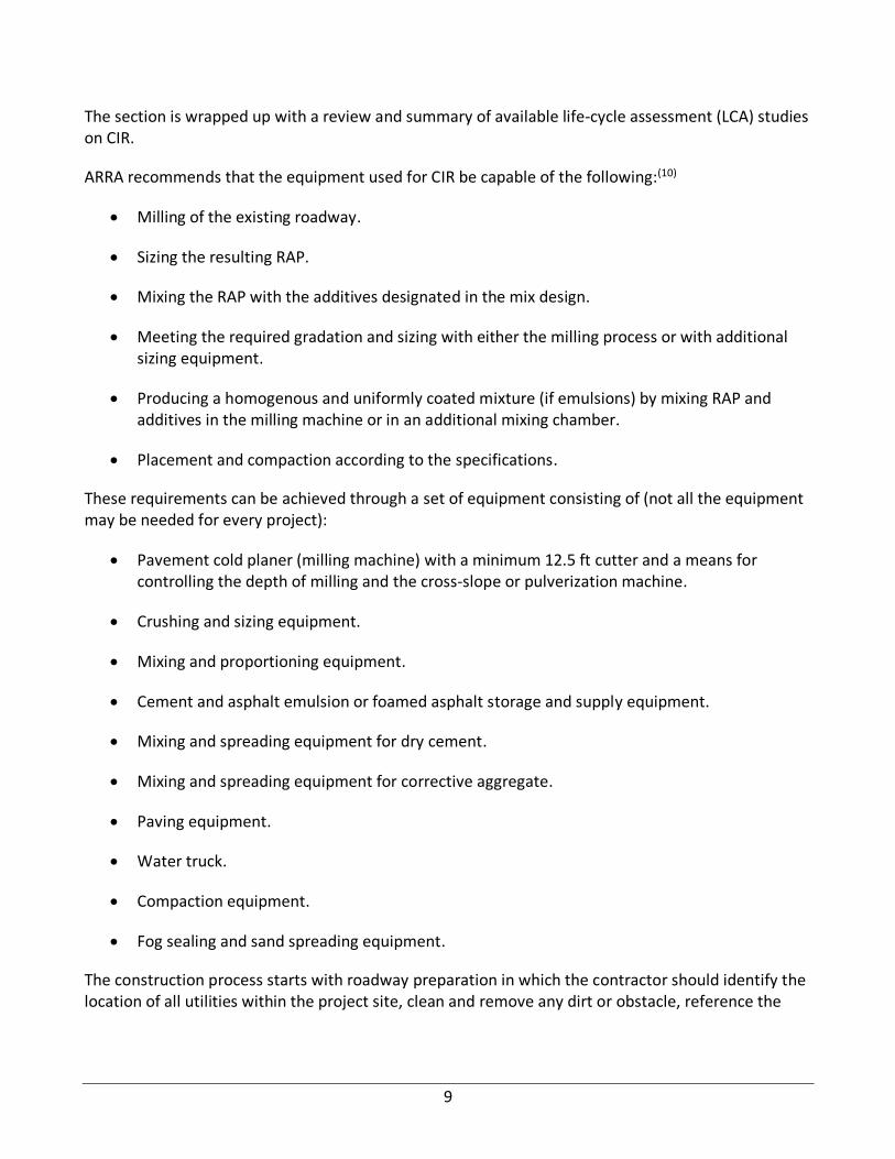
ARRA recommends that the equipment used for CIR be capable of the following:(10)

• Milling of the existing roadway.

• Sizing the resulting RAP.

• Mixing the RAP with the additives designated in the mix design.

• Meeting the required gradation and sizing with either the milling process or with additional sizing equipment.

• Producing a homogenous and uniformly coated mixture (if emulsions) by mixing RAP and additives in the milling machine or in an additional mixing chamber.

• Placement and compaction according to the specifications.

These requirements can be achieved through a set of equipment consisting of (not all the equipment may be needed for every project):

• Pavement cold planer (milling machine) with a minimum 12.5 ft cutter and a means for controlling the depth of milling and the cross-slope or pulverization machine.

• Crushing and sizing equipment.

• Mixing and proportioning equipment.

• Cement and asphalt emulsion or foamed asphalt storage and supply equipment.

• Mixing and spreading equipment for dry cement.

• Mixing and spreading equipment for corrective aggregate.

• Paving equipment.

• Water truck.

• Compaction equipment.

• Fog sealing and sand spreading equipment.

The construction process starts with roadway preparation in which the contractor should identify the location of all utilities within the project site, clean and remove any dirt or obstacle, reference the

10

profile and cross-slope, cold mill along cross walks and gutters to prepare for the final overlay, and correct all areas known to have soft or yielding subgrades.

CIR construction is recommended only when the existing pavement temperature is above 50°F and the previous overnight temperature is above 35°F. A control strip with a minimum length of 1000 ft should be constructed on the first day of the project to show that the construction process meets the specifications. The optimal rates of additives (if any) and the rolling pattern to achieve the optimum field density should be identified from the control strip.

The existing pavement should be milled to the depth required by the plan or the specifications, and the recycled materials should be crushed and sized to the maximum particle size specified.(10) Typical depths are 2 to 4 in. The incorporation of recycling additive or stabilizing agent can be in the form of applying mechanical, chemical, or bituminous additives or a combination of all.(11) Mechanical stabilization in the form of compaction is used for all treatments, and the addition of imported granular materials is used if the existing in-place materials do not provide a satisfactory gradation. Chemical stabilization is achieved by adding one or a combination of Portland cement, fly ash, calcium chloride, magnesium chloride, and lime. Bituminous stabilization consists of adding asphalt emulsion or foamed asphalt. The common practice in many states is to use a combination of bituminous stabilization and chemical stabilization for partial-depth recycling.(11) Cement or lime slurry may be directly added to the mixing chamber or sprayer over the cutting teeth of the milling machine.(11) If dry cement or corrective aggregate is needed, it can be spread on the existing surface before milling. The CIR milling and mixing process can be accomplished with a single-unit machine or a multi-unit train.

The placement of the recycled materials is conducted either with conventional asphalt pavers or cold mix pavers followed by compaction. The time between material placement and start of compaction is determined by the contractor. Compaction (initial/breakdown, intermediate, and final compaction) is one of the main factors affecting the future performance of the section. The type and number of compactors depend on many factors such as the degree of compaction required, material properties of the pulverized mix, support capabilities of the underlying layers, and the needed productivity.(11) In general, the characteristics of the recycled mix determine the type of roller needed and the thickness of the layer, and the required compaction dictates the weight, amplitude, and frequency of the compactors.

For materials stabilized by some chemical and/bituminous materials, in a process similar to that shown in Figure 7 and Figure 8, curing is a critical step and is needed to assure achieving adequate strengths before opening to traffic, prevent raveling, and facilitate placement of the final wearing course.(11,12,13) The curing rate depends on multiple factors such as the nature of the stabilization, particularly if asphalt emulsions are used, temperature, humidity, moisture content of the mix, compaction level, and drainage characteristics of the section.

ARRA requires CIR to cure for a minimum of three days and the moisture content to be less than 3% before proceeding to secondary compaction or opening to traffic.(10) ARRA recommends secondary compaction if the recycling agent is emulsified asphalt. If secondary compaction is planned, a separate rolling pattern should be established during the control strip and the density of the recycled

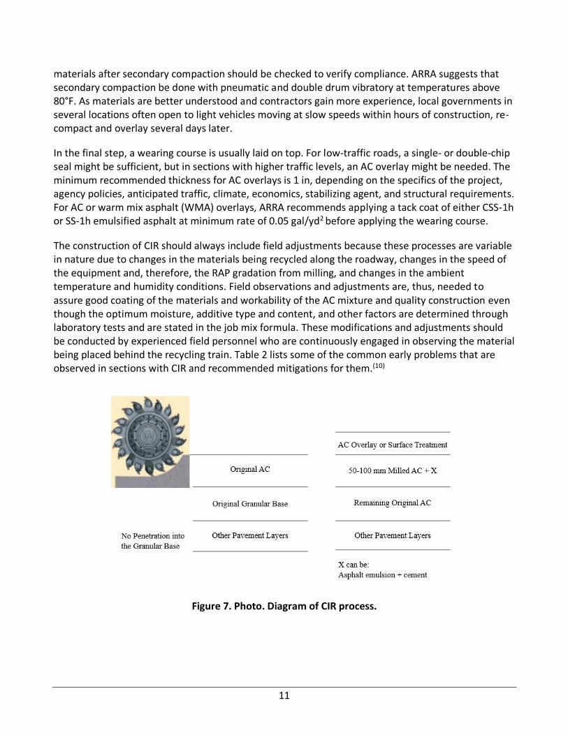
11

materials after secondary compaction should be checked to verify compliance. ARRA suggests that secondary compaction be done with pneumatic and double drum vibratory at temperatures above 80°F. As materials are better understood and contractors gain more experience, local governments in several locations often open to light vehicles moving at slow speeds within hours of construction, re-compact and overlay several days later.

In the final step, a wearing course is usually laid on top. For low-traffic roads, a single- or double-chip seal might be sufficient, but in sections with higher traffic levels, an AC overlay might be needed. The minimum recommended thickness for AC overlays is 1 in, depending on the specifics of the project, agency policies, anticipated traffic, climate, economics, stabilizing agent, and structural requirements. For AC or warm mix asphalt (WMA) overlays, ARRA recommends applying a tack coat of either CSS-1h or SS-1h emulsified asphalt at minimum rate of 0.05 gal/yd2 before applying the wearing course.

The construction of CIR should always include field adjustments because these processes are variable in nature due to changes in the materials being recycled along the roadway, changes in the speed of the equipment and, therefore, the RAP gradation from milling, and changes in the ambient temperature and humidity conditions. Field observations and adjustments are, thus, needed to assure good coating of the materials and workability of the AC mixture and quality construction even though the optimum moisture, additive type and content, and other factors are determined through laboratory tests and are stated in the job mix formula. These modifications and adjustments should be conducted by experienced field personnel who are continuously engaged in observing the material being placed behind the recycling train. Table 2 lists some of the common early problems that are observed in sections with CIR and recommended mitigations for them.(10)

Figure 7. Photo. Diagram of CIR process.

12

Figure 8. Photo. Diagram of CIR equipment.

Table 2. CIR Early Damage and Mitigation

Distress Mitigation

Isolated areas of minor raveling or scuffing. Sweep and monitor. Determine if fog sealing or re-fog sealing is necessary to protect.

Isolated areas of major raveling, scuffing, or tearing.

Maintain better traffic restrictions in areas that are not cured. Sweep and monitor. Determine if fog sealing or re-fog sealing is necessary to protect. Fill or remove and replace deep damaged areas with AC mixture (cold mix, recycled mix, WMA, or traditional AC) prior to surface course.

Large scale areas of raveling, scuffing, or tearing in straight traffic areas.

Re-recycle or remove and replace with asphalt mixture (cold mix, recycled mix, WMA, or AC).

Dimpling due to parked vehicles or equipment. Fill with AC mixture (cold mix, recycled mix, WMA, or traditional AC) prior to surface course.

Permanent deformation within wheel path areas due to secondary compaction by traffic.

If pavement temperatures permit, apply secondary compaction. Fill with AC mixture (cold mix, recycled mix, WMA, or traditional AC) or micro surfacing in the low areas or cold mill to provide a smooth surface.

Permanent deformation and shoving due to unstable mix.

Investigate pavement structure in conjunction with mix design lab. Depending on investigation, remove and replace affected areas with AC mixture (cold mix, recycled mix, WMA, or traditional AC) or re-recycle supplementing with uncoated coarse aggregate, additives and/or recycling agent as necessary.

Full-Depth Reclamation

The FDR construction process is similar to CIR; the only difference, as stated earlier, is that the whole thickness of the existing AC layer and a predetermined thickness of the underlying layer for at least 2 in are pulverized and mixed together (with water and with or without additives) into a homogenous mixture, as shown in Figure 9 and Figure 10.(12,13)

13

FDR can recycle pavement depths up to 12 in. The FDR process can vary between projects, depending on the project specifics, owner/agency needs, and the requirements of the section after recycling.(15) The common practice for many agencies is to use a combination of foamed asphalt and chemical stabilization (typically cement) or only chemical stabilization or only asphalt emulsion stabilization with FDR.

Figure 9. Photo. Diagram of FDR process.

Figure 10. Photo. Diagram of FDR equipment.

ARRA has set the requirements shown in Table 3 on the gradation of the FDR pulverized material.(12) When using asphalt emulsion, the maximum passing sieve no. 200 should not exceed 20%.(14) Research conducted at University of California Pavement Research Center (UCPRC) recommends less than 12% passing the no. 200 sieve for stabilization with a combination of foamed asphalt and cement and up to 15% maximum with special consideration for binder content.

14

Table 3. ARRA Requirements on FDR Recycled Materials Gradation

Sieve Size Minimum Percent Passing

3 in (75 mm) 100

2 in (50 mm) 95

No. 4 (4.75mm) 55

No. 200 (0.075 mm) 5

For compaction of FDR with bituminous stabilization, ARRA requires the processed materials to be uniformly compacted in one layer. (12) The moisture content at the start of the compaction should be within −1 percent to +2 percent of the specified optimum moisture. The initial compaction should not be more than 500 ft (160 m) behind the reclaimer unit and should be done by a padfoot or pneumatic roller. After the breakdown roller, the materials should be spread using a motor grader until the desired shape and slope are achieved. After blading, a vibratory double drum steel roller and pneumatic roller should be used for intermediate and final compaction of the layer. Completed portions can be immediately opened to low-speed local traffic. The overlay should follow within several days to protect the recycled layer from traffic wear.

For stabilization with cement, ARRA recommends that no more than 60 minutes pass between the first contact of cementitious stabilizer with water and application on the subgrade, and the time span between placement of the stabilizer and start of mixing not exceed 30 minutes. (15) Compaction should begin no more than 20 minutes after mixing, and all compaction operations should be completed within 2 hours from the start of the mixing process. There should be no grading or blading of the material after compaction has been completed. Curing is done by application of a bituminous or other approved sealing membrane or by using water spray to keep the section moist for three to five days. To help limit shrinkage cracking, micro-cracking can be done (optional) by using a 12 ton steel wheel vibratory roller. Completed portions of the section can be immediately opened to low-speed local traffic.

The key for quality FDR construction, as identified by a UCPRC report on guidelines for in-place recycling, is the following:(14)

• Contractor experience.

• Traffic accommodation.

• Pre-milling in cases where the asphalt layer is too thick (typically more than 10 in) or when precise surface levels need to be maintained.

• Importing new material in case additional materials are needed to correct grades, increase layer thickness, and/or improve the bearing capacity of the section.

• Equipment inventory.

• Recycling train crew responsibilities.

15

• Recycling train setup.

• Test strip to check processes and determine compaction rolling pattern necessary to achieve specified density.

• Ambient and pavement temperatures for asphalt emulsion additives (it is recommended to start the recycling when the ambient temperature is over 50ºF and the temperatures of the road surface and pre-spread active filler are both equal of above 60ºF).

• Recycling plan.

• Recycling additive content and application rate.

• Recycling depth and recycled material consistency.

• Lateral joints.

• Compaction moisture.

• Initial compaction, final grades, and final compaction.

• Curing.

• Trafficking.

• Surfacing.

• Drainage.

• Quality control.

FHWA has published checklists for CIR and FDR in collaboration with the ARRA and the National Center for Pavement Preservation.(16,17) The checklists are comprehensive and include items for document review, project review, materials checks, preconstruction inspection responsibilities (preconstruction meeting, surface preparation, and equipment inspection), weather requirements, mix design, traffic control, project inspection responsibilities (milling, crushing, mixing, pickup machine and paver, rolling procedure, and quality assurance), opening to traffic, curing, and surface course.

Energy Use and Emissions

There are a few studies that have tried to estimate energy consumption and emissions of in-place recycling techniques. Although the number of studies is limited, they all result in the same conclusion: CIR not only reduces consumption of virgin materials, but also results in significant savings in energy consumption and emission compared to conventional methods of rehabilitation.

16

Thenoux compared the energy consumption during construction for three different structural pavement rehabilitation alternatives, which included AC overlay, reconstruction, and FDR-foamed asphalt.(18) It was determined that the FDR technique is the least energy consuming in all the scenarios, resulting in energy savings between 20% to 50% compared to AC overlay and up to 244% compared to reconstruction.

Robinette and Epps conducted a literature survey for estimating energy consumption and emissions of IPR practices.(19) The results are presented in Table 4 and Table 5.(19)

Table 4. Energy Consumption (Btu/yd2-inch) for CIR Processes

Operation NCHRP 214 Colas Group PaLATE Granite Construction Representative Range

CIPR—partial depth — 6,400 24,600 3,100 3,000–24,000

CIPR—full depth 15,000–20,000 6,200 34,700 1,300–11,100 1,300–15,000

Table 5. GHG Emissions (CO2-eq. lb/yd2-inch) of Different CIR Processes

Operation Colas Group Granite Construction Representative Range

Cold milling asphalt pavement 0.084 3.377 0.08-3.500

CIPR—partial depth — 0.71 —

CIPR—full depth 1.082 0.932-4.017 0.900-4.100

17

CHAPTER 3: GOAL AND SCOPE SUMMARY

GOAL OF THE STUDY

The goal of the study is to develop a LCA methodology to assess the environmental impacts and energy use of transportation projects that involve maintenance and rehabilitation treatments using in-place recycling and conventional paving methods.

SCOPE OF THE STUDY

The scoping elements include the methodological choices required at the Goal and Scope phase of LCA according to the ISO 14044 and FHWA pavement LCA framework.(1,2)

Functional Unit

The functional unit used in this LCA study is a one lane-mile over the analysis period. The analysis period depends on the treatments under comparison. The lane width is assumed to be equal to 12 ft.

System Boundary

The product systems included in the study are in-place recycling methods recognized by federal and state transportation agencies in the United States, which will be compared with conventional hot-mix asphalt (HMA) overlays. The LCA includes the following life-cycle stages: material production, construction, maintenance, use, and end of life. The material production and construction life cycles of the systems considered in this LCA are related to in-place recycling or conventional mill/fill processes. Thus, any processes related to the production and construction of the initial pavement is not included. The system boundary for the product system is shown as the dashed line in Figure 11.

Figure 11. Chart. Life-cycle phases and system boundary of the LCA scope.

Analysis Period

The analysis period is calculated following the method highlighted in the FHWA pavement LCA framework.(1) This method compares the life expectancy of treatments under study, defines the

18

alternative treatment with the longest life expectancy, and adds it to the estimated life of the subsequent maintenance of the longest living treatment, as illustrated in Figure 12. It is important to assign a common analysis period to compare the pavement rehabilitation alternatives and to quantify the impacts of the use stage.

Figure 12. Graph. Analysis period strategy illustrating the first treatment’s lifetime to be analyzed by the tool and subsequent overlays.

Allocation Method

The adopted allocation method is the cut-off, also known as recycled content methodology.(20) The boundary of the analysis conducted is limited to the pavement system during the analysis period without accounting for the quantity of resources used in a subsequent system. The substitution allocation method is analyzed in the interpretation step of the LCA methodology to compare its effect to the cut-off method.

INVENTORY ANALYSIS AND IMPACT CATEGORIZATION

Inventory database is compiled from primary and secondary sources with regionalized data collected from agencies and contractors from the three main US regions. Life-cycle inventory analysis is performed using regionalized models for fuel and electricity. More details about life-cycle inventory are provided in Chapter 4.

The impact characterization is performed using the EPA’s Tool for Reduction and Assessment of Chemicals and Other Environmental Impacts (TRACI) categories. Four quantitative outcomes from the LCA study are: global warming potential, energy, total energy with feedstock, and single score.

0 10 20 30 40 50 60

1

2

3

4

5

Years

Mai

nte

nan

ce o

r re

hab

iluta

oti

on

alt

ern

ativ

es

Rehabilitation

AC Overlay 1

AC Overlay 2

AC Overlay 3

Analysis period

19

Global Warming Potential

“Global warming is an average increase in the temperature of the atmosphere near the Earth’s surface and in the troposphere, which can contribute to changes in global climate patterns. Global warming can occur from a variety of causes, both natural and human induced. In common usage, global warming often refers to the warming that can occur as a result of increased emissions of greenhouse gases from human activities.”(21) This impact is given in units of kg carbon dioxide equivalence (CO2e). The 100-year GWP is calculated using the EPA’s TRACI 2.1.

Single Score

Other environmental impacts were reported in a condensed format though calculation of a unitless parameter based on the normalization and weighting for TRACI impacts using the coefficients presented in Table 6.(22,23) This parameter is referred to as the Single Score, which is reported in “points.” It must be noted that the weighting given to the Single Score is subjective, though the weighting values developed by the National Institute of Standards and Technology (NIST) are specific to the context of the United States.

Table 6. TRACI Impacts with Normalization and Weighting Factors

Impact Category Unit Normalization Weighting

Ozone depletion kg CFC-11 eq 6.20 0.024

Smog kg O3 eq 0.000718 0.048

Acidification kg SO2 eq 0.0110 0.036

Fossil fuel depletion MJ surplus 0.0000579 0.121

Eutrophication kg N eq 0.0463 0.072

Respiratory effects kg PM2.5 eq 0.0412 0.108

Non carcinogenics CTUh 952 0.060

Carcinogenics CTUh 19,706 0.096

Ecotoxicity CTUe 0.0000905 0.084

Global warming kg CO2 eq 0.0000413 0.349

Energy Indicators

Two energy consumption indicators are included in the impact assessment: energy and total energy with feedstock. Energy refers to combusted or expended energy as fuel. Total energy with feedstock includes energy that is embodied as a fuel (e.g., diesel, natural gas) and energy that is embodied as a material (e.g., plastics, asphalt binder). As FHWA pavement LCA guidelines recommend, two types of energy are reported to provide a more complete view of energy consumption over the life cycle.(1) For example, accounting feedstock energy for asphalt agents results in higher energy for asphalt concrete pavement life cycle due to the energy retained in the asphalt binder.

20

CHAPTER 4: LIFE-CYCLE INVENTORY ANALYSIS

DATA COLLECTION

The data collection phase of the study included collecting primary and secondary data from various sources. Primary data refer to specific data collected for some of the in-place recycling techniques from contractors, whereas secondary data refer to average and background data for processes like fuel and electricity production, and emissions due to equipment use. Data sources included agency and contractor questionnaires and interviews, commercial inventory databases, and publicly available data sources.

Primary Data

The primary data are the information collected from field projects and used for quantification of life-cycle inventory (LCI) impacts. Questionnaires have been distributed to contractors throughout the United States in 2016–2017. Data collection was undertaken at an early stage of the project to collect information and data about in-place recycling (IPR) techniques and construction methods. The project information and data were analyzed to assess the fuel usage of IPR techniques, especially CIR and FDR. Follow-up interviews were conducted with some of the contractors to collect additional data.

Figure 13 represents the distribution of agencies and contractors that responded to questionnaires and shared their IPR data from field projects.

Figure 13. Photo. Representative map of contractors and agencies contacted in three main US regions.

Appendix A contains information collected from agencies regarding HIR and CIR/FDR practices. The main conclusions extracted from the data collected are that IPR techniques are applied under specific project conditions. The selection of any IPR type requires a good understanding of the dynamic parameters (traffic level, truck percent, lane closures and openings, and climate) and static characteristics (road geometry, structural capacity, and existing pavement condition). It was found that HIR and CIR are commonly used at low traffic volume pavements, under a truck percent that

21

varies from 5% to 10% for a pavement length of 100 lane-mile per year. According to agencies’ responses, CIR extends existing pavement service life to more than 11 years, whereas HIR is reported to extend service life from five to ten years. The difference in performance between CIR/FDR and HIR is because CIR/FDR is a rehabilitation technique that enhances the structural capacity and treats a wide range of surface and deep distresses. In contrast, HIR is classified as a maintenance treatment applied to a limited number of functional distresses.

Fuel Usage Models for IPR Techniques

This section presents the various construction practices of IPR treatments and their energy analysis during the construction stage of the life cycle. In the construction stage, the processes are mainly associated with fuel usage of equipment used in construction. The main factors that affect energy use are discussed, evaluated, and quantified to measure their impact on the construction stage of each treatment. The construction processes modeled represent specific construction projects. The in-place recycling techniques are introduced and discussed separately.

Hot In-Place Recycling

General HIR Process

In this study, the milling depth during HIR construction processes is assumed 1.5–1.75 in for resurfacing and 1–3 in for remixing and repaving. The construction information of the HIR treatments was based on data collected from projects in various locations. The total propane consumption ranges from 118.17 to 253.46 gal/hour for resurfacing and from 138.55 gal/hour to 1030.73 gal/hour for remixing and repaving. The equipment propane consumption was based on an average train speed of 18.5 ft/minute. Figure 14 shows that most of the HIR projects consumed approximately 323 gal/hour of propane fuel. According to the results in Table 7, the energy consumption of HIR resurfacing, HIR remixing, and HIR repaving construction operations were found to be 95.95GJ/lane-mile, 242.56GJ/lane-mile, 250.56 GJ/lane-mile, respectively.

Figure 14. Graph. Histogram of HIR projects propane consumption.

0 5 10 15 20 25 30 35 40

118.2

323.0

527.7

732.5

937.3

1142.1

1346.8

More

Frequency

Tota

l H

IR t

ota

l p

rop

an

e

con

sum

pti

on

(g

al/

hou

r)

22

Table 7. Details for the Environmental Assessment of HIR Construction Processes

Activity Equipment Type Fuel Type HP Hourly Fuel Consumption (Gal/hour)

Speed (ft/minute)

Total Energy (GJ/Lane-mile)

HIR Surface Recycling Preheater Diesel 99 3 18.5 95.95

HIR Surface Recycling Heater/Scarifier Unit Diesel 321 3 18.5 –

HIR Surface Recycling Preheater Propane 99 106 18.5 –

HIR Surface Recycling Heater/Scarifier Unit Propane 321 71 18.5 –

HIR Surface Recycling Vibratory Roller Diesel 150 8.1 25 –

HIR Remixing Preheater Diesel 99 3 18.5 242.56

HIR Remixing Heater/Mixer Unit Diesel 321 3 18.5 –

HIR Remixing Preheater Propane 99 286 18.5 –

HIR Remixing Heater/Mixer Unit Propane 321 190 18.5 –

HIR Remixing Vibratory Roller Diesel 150 8.1 25 –

HIR Repaving Preheater Diesel 99 3 18.5 250.65

HIR Repaving Heater/Scarifier or Mixer Unit

Diesel 321 3 18.5 –

HIR Repaving Preheater Propane 99 286 18.5 –

HIR Repaving Heater/Scarifier Unit Propane 321 190 18.5 –

HIR Repaving Vibratory Roller Diesel 150 8.1 25 –

HIR Repaving Paver Diesel 250 10.6 18.5 –

The energy use results calculated for each HIR treatment are shown in Figure 15 separated by fuel type and equipment type. Repaving has the highest amount of energy use among all HIR treatments because it has an additional paving activity of an asphalt overlay. The equipment used to heat the pavement surface (preheater, heater/scarifier unit, and heater/mixer unit) contributes the most to energy consumption due to their high propane consumption. The heating machines contribute 90.45%, 96.22%, and 93.12% to overall energy consumption for resurfacing, remixing, and repaving, respectively.

23

Figure 15. Graph. Construction energy consumption of HIR methods.

Effect of Air Temperature

The HIR projects analyzed were constructed in air temperature that ranges from 34°F to 87°F. The data analysis within this range showed that air temperature does not have any effect on propane consumption of the heating machines, as it did not show any consistent trend. However, it was clear that the highest propane consumption rates were localized in the range between 68°F and 87°F, which falls in the range of the construction season temperatures that usually start in April and end in October (Figure 16).

Figure 16. Graph. The HIR total propane consumption versus air temperature for US states.

0

20

40

60

80

100

120

140

Vib

rato

ry R

oll

er

Pre

hea

ter

Hea

ter/

Mix

er U

nit

Vib

rato

ry R

oll

er

Pav

er

Pre

hea

ter

Hea

ter/

Mix

er U

nit

Vib

rato

ry R

oll

er

Pre

hea

ter

Hea

ter/

Sca

rifi

er U

nit

HIR

Remixing

HIR Repaving HIR Surface

Recycling

Tota

l E

ner

gy(

GJ/

lan

e-m

ile)

Propane Fuel

Diesel Fuel

0

100

200

300

400

500

600

700

50 57 58 65 70 75 78 79 80 82 83 85 87

To

tal

pro

pan

e co

nsu

mp

tio

n (

gal/

hou

r)

Average air temperature (ºF)

Illinois

New Jersey

Tennessee

Wisconson

California

Construction Season

IL

NJ

TN

WI

CA

24

Effect of Construction Year

According to the results presented in Figure 17, the data collected from contractors between 2012 and 2014 show that the average propane consumption of the projects analyzed decreases. That decrease might be due to the use of a lower number of equipment units or change in the operation of trains. Propane consumption decreased 44.75% from 2012 to 2013 and 49.05% from 2013 to 2014.

Figure 17. Graph. Total HIR propane consumption versus year of construction.

Effect of Equipment Type

In 2014, heater units used to operate HIR construction activities and the projects analyzed were either tractor pulled or self-propelled. The tractor-pulled set is an equipment train propelled by a tractor truck; thus the speed of the equipment train units depends on the speed of the tractor truck. The self-propelled or self-contained equipment is defined as “automobiles, motorcycles, aircraft, boats, snowmobiles, trucks, tractors, jet skis, lawn mowers, golf carts, etc., that convert their own energy supply into motive power used for propulsion.”(24) Figure 18 shows that in 2014, the self-propelled heater unit consumed 11.71% less propane than the tractor-pulled set. Therefore, it is more efficient to use self-propelled instead of tractor-pulled heating machine units.

0

200

400

600

800

2012 2013 2014

Tota

l p

rop

ane

con

sum

pti

on

(gal

/hour)

Construction year

25

Figure 18. Graph. HIR propane consumption for two equipment sets.

Effect of Milling Depth

The first step in the HIR construction process is to heat the milling depth of the pavement surface to soften it before milling. Figure 19 shows that the higher the milling depth for both resurfacing and remixing, the greater the propane consumption. For remixing, propane consumption ranges from 154 gal/hour to 689 gal/hour for a milling depth varying from 1 to 2 in. Whereas the propane consumption of resurfacing varies from 175 gal/hour to 206 gal/hour at milling depth of 1.5 and 1.75 in, respectively.

Figure 19. Graph. Total propane consumption of HIR resurfacing and HIR remixing versus milling depth.

Effect of Pavement Aggregate Hardness

Pavement aggregate hardness is one of the main factors that influence propane and diesel fuel consumption. This study considers the impact of pavement hardness on propane consumption because propane usage has the highest contribution to overall energy use. The impact of pavement hardness is mostly seen during the scarification or grinding of the existing HMA surface. Hardness can be attributed to aggregate type, temperature during heating, and asphalt binder type used in the

145 150 155 160 165 170 175 180 185

Self-propelled

Tractor pulled

Propane consumption (gal/yd2)

0

200

400

600

800

1.5 1.75 1 1.25 1.5 2

Resurfacing Remixing

Tota

l p

rop

an

e c

on

sum

pio

n

(ga

l/h

ou

r)

Milling depth (inch)

26

surface layers. The project-specific data collected from the contractors were used to evaluate the effect of hardness with an intent to develop a model that can predict the relative hardness of the pavement based on project location.

Available data show propane consumption during the remixing process in different job locations in Georgia, Illinois, Massachusetts, New Jersey, Tennessee, and Wisconsin. In order to characterize the aggregate hardness at these locations, the average Mohs hardness (0–10) was defined for each state based on the predominant aggregate types found in these states according to a US Geological Survey (USGS) study illustrated in Figure 20. (25) For instance, the predominant rock type in Illinois and Tennessee is limestone, so the average Mohs hardness associated to their job locations is 3.5.(25) Granite and limestone are the predominant rocks in Wisconsin and Georgia, so their associated average Mohs hardness is 5.5. Granite and sandstone are the predominant rocks in New Jersey and Massachusetts, and their average Mohs hardness is 6.5. Based on the primary data collected about HIR remixing job locations, the average propane consumption in Illinois, Tennessee, Wisconsin, Georgia, New Jersey, and Massachusetts are 0.15 gal/yd2, 0.16 gal/yd2, 0.47 gal/yd2, 0.56 gal/yd2, 0.58 gal/yd2, and 0.86 gal/yd2, respectively. The results summarized in Table 8 show that pavements containing harder aggregates result in higher propane consumption during the remixing process.

Figure 20. Photo. Generalized locations of aggregate resources.

Table 8. Average Mohs hardness of the available HIR remixing job locations.

State Predominant rock types Average Mohs hardness (0-10) Propane consumption (gal/yd2)

Wisconsin Granite, limestone 5.5 0.47

Georgia Granite, limestone 5.5 0.56

New Jersey Granite, sandstone 6.5 0.58

Massachusetts Granite, sandstone 6.5 0.86

Illinois Limestone 3.5 0.13

Illinois Limestone 3.5 0.12 Illinois Limestone 3.5 0.17



Tennessee Limestone 3.5 0.16

27

A linear regression analysis is performed to predict the propane consumption of the heating machines set (Preheater + Heater/Mixer unit) during the remixing construction process based on the available data. The independent variable in this analysis is the relative Mohs hardness. Table 9 shows the results of the regression. The predictor variable has a high significance (p-value < 0.001) and the model coefficient of determination (R2) is 0.923. This best fit model is shown below and can be applied by different states to estimate the total propane consumption.

Table 9. HIR Remixing Propane Consumption Regression Model Results

Regression parameters Coefficients Standard error T-value P-value

Intercept −0.5072 0.0896 −5.657 0.0005

Average Mohs hardness 0.1879 0.0192 9.795 9.96e-06

R2 = 0.923 - - - -

The effect of aggregate hardness on propane consumption during the remixing construction process was analyzed in California and Illinois. The average Mohs hardness for the aggregates in California is 6.5 because the predominant rocks are trap, sandstone, and granite; whereas, the average Mohs hardness for the aggregates in Illinois is 3.5, because the predominant rock is limestone. Therefore, based on the developed linear regression mode, the total energy resulting from propane consumption is 570.02 and 127.28 GJ/lane-mile in California and Illinois, respectively. As a result, HIR treatment can be less efficient in California than in Illinois.

Cold In-Place Recycling

General CIR Process

According to the information collected from contractors in 2015, two different construction methods commonly used for CIR were single machine and the single-pass equipment train.

The single machine method breaks, pulverizes, and adds recycling agents in a single pass.(26) The advantages of a single machine include high production capacity and simplicity of operation. In contrast, the single-pass equipment train consists of a cold milling machine, a portable crusher, a travel-plant mixer, and a laydown machine.(26) It provides better process control, more uniformity, and higher production rates (often more than two miles per day).

An environmental impact assessment is conducted for CIR operations. In this study, the milling depth during CIR construction processes ranges from 3 to 4 in. The construction information of CIR was based on the data collected from 24 projects located in Illinois, Indiana, Iowa, Massachusetts, and Nebraska that used the single-pass equipment train method. The equipment fuel consumption was based on an average train speed of 22 ft/minute. The fuel consumption of the equipment used in CIR processes is presented in Table 10. The milling operation contributes the most in the total energy of the CIR construction process with approximately 82.32%.

Figure 21 shows that most of the CIR projects consumed approximately 0.04 gal/yd2 of diesel, which also matches the total fuel consumption calculated for the CIR single-pass equipment train 0.036 gal/yd2 in Table 10, thus resulting in a total of 58.628 GJ/lane-mile energy use.

28

Figure 21. Graph. Histogram of CIR projects total diesel consumption.

Table 10. Details for the Environmental Assessment of CIR

Equipment type HP Average fuel consumption (gal/yd2)

CIR energy (GJ/Lane-mile)

Milling machine 860 0.01966 48.260

Crusher/pugmill 375 0.00488 4.792

Oil pump 5 0.00005 0.002

Paver 150 0.00204 2.000

Pickup machine 90 0.00126 1.238

Skid steer 70 0.00019 0.186

Double steel drum roller 115 0.00128 1.255

Rubber tire roller 150 0.00081 0.802

Water truck 425 0.00027 0.011

Pickup truck 300 0.00448 0.061

Service truck 300 0.00154 0.021

Total - 0.03646 58.628

Effect of Air Temperature

The University of Leeds conducted a study on the “impact of ambient temperatures on exhaust thermal characteristics during cold start.”(27) The study showed that ambient temperatures have an impact on fuel consumption and that 1.4% more fuel was consumed in a cold winter (28.4°F) compared with a hot summer (87.8°F) because of the higher heat losses caused by increased mechanical frictions in the vehicle engine. A study investigated the relationship of combustion efficiency of direct injection diesel engine as function of time cold and warm conditions.(28) It was found that for the warm start of the engine, the efficiency was over 98%; whereas, the efficiency did not exceed 95% at cold start. Figure 22 shows that the diesel consumption of the CIR projects analyzed has a decreasing trend with higher air temperatures. In addition, the cutting speed during the milling operation increases under warmer temperatures.

0 2 4 6 8 10 12 14

0.02

0.04

0.06

More

Frequency

Tota

l C

IR d

iese

l co

nsu

mpti

on

(gal

/yd

2)

29

Figure 22. Graph. Effect of air temperature on diesel consumption and cutting speed during milling operation.

Effect of Pavement Width

During the follow-up interviews with the contractors, it was found that pavement width is another factor affecting fuel consumption during the milling operation. The CIR contractors typically used a half-lane milling machine model characterized by a cut width of 12.5 ft. Figure 23 shows that the wider the pavement lane, the more diesel is consumed by the milling machine and the higher is the number of teeth per 100 ton used in the milling operation. In fact, the contractor needs to change the number of installed cutting teeth for different widths.

Figure 23. Graph. Total CIR fuel consumption versus width.

0

5

10

15

20

25

30

0

0.01

0.02

0.03

0.04

0.05

0.06

62 68 71 77 79 84 87 89

Aver

age

cut

spee

d (

ft/m

in)

Aver

age

die

sel

con

sum

pti

on

(gal

/yd

2)

Average air temperature (ºF)

Fuel consumption Cut speed

Linear (Fuel consumption) Linear (Cut speed)

0

1

2

3

4

5

6

7

8

0

0.005

0.01

0.015

0.02

0.025

0.03

11 12 13

Num

ber

of

tooth

per

ton

Aver

age

mil

ling d

iese

l co

nsu

mp

tion

(gal

/yd

2)

Pavement width (ft)

Milling fuel consumption Number of tooth per 100 ton

30

A multiple regression analysis was performed to predict the diesel consumption of the milling machines set (milling machine + crusher) during the CIR construction process based on available data. The independent variables in this model are pavement width and the number of teeth per 100 tons. The predictor variable has a high significance (p-value <0.001) and the model R2 is 0.81. The best fit model obtained is given in Table 11 and can be used to estimate the fuel consumption during the milling operation of CIR.

Table 11. CIR Milling Operation Fuel Consumption Regression Model

Regression Parameters Coefficients Standard Error T-Value P-Value

Intercept −0.0343 0.0482 −0.711 0.4949

Width 0.0039 0.0047 0.950 0.3668

Teeth per 100 tons 0.0017 0.0003 6.005 0.0002

R2 = 0.8063 - - - -

Effect of Milling Depth

The effect of milling depth on fuel consumption has been investigated. Figure 24 shows that the total fuel consumption increases with higher milling depth. However, there is no clear trend of crushing and milling fuel consumption rates with increasing milling depth. In the range from 3.5 to 5 in cut depth, the milling fuel consumption is clearly increasing, but the crushing contribution stays at approximately a constant rate from 3 to 5 in.

Figure 24. Graph. CIR Diesel consumption versus milling depth.

0

0.005

0.01

0.015

0.02

0.025

0.03

0.035

0.04

0.045

0.05

3 3.5 4 5

Aver

age

die

sel

con

sum

pti

on

(g

al/y

d2)

Milling depth (inch)

Total fuel consumption Milling fuel consumption Crushing fuel consumption

31

Effect of Equipment Technology

Higher horsepower results in higher fuel consumption.(29) The CIR contractor used two types of equipment trains that differ in their milling machine horsepower (HP).(26) Train 1 has a milling machine of HP equal to 800 and train 2 is characterized by a milling machine of HP equal to 860. Table 12 shows that HP of 860 results in a fuel consumption higher than HP of 800 with a difference of 4%.

Table 12. Summary of HP Effect on Fuel Efficiency

Train type Train 1 (Milling machine, HP= 800) Train 2 (Milling machine, HP= 860)

Diesel consumption (gal/yd2) 0.0197 0.0205

Fuel Use for Conventional Overlay Methods

The fuel usage data for conventional overlays were extracted from Tollway pay items. According to results of Figure 25, HMA full-depth projects construction total consumption is higher than the HMA surface and base courses.(30) In Figure 26, the contribution of equipment unit used in 12-in thick full-depth HMA was assessed and it was found that the milling machine contributes the most to the overall construction processes fuel consumption, followed by paver and then different roller types.

Figure 25. Graph. Fuel consumption of conventional overlay projects.

0

0.05

0.1

0.15

0.2

0.25

HMA (full depth), 12 in HMA (full depth), 15 in HMA base course, 4 in HMA surface course, 3 in

Aver

age

fuel

con

sum

pti

on

(g

al/y

d2)

32

Figure 26. Graph. 12-in full-depth HMA overlay equipment use contribution.

Secondary Data

The secondary data complement the inventory items missing in the primary data collected. Various sources were used to compile a comprehensive inventory list which are: (1) commercial LCI databases (e.g., Ecoinvent 2.2/3.0, U.S.-Ecoinvent 2.2), (2) software (e.g., EPA MOVES 2014, eGRID 2010), (3) governmental databases, (4) governmental reports, (5) material safety data sheets, and (6) equipment manufacturer specifications.(31,32,33,34,35)

Other Data Collected from Questionnaires (States)

Apart from primary data collected from contractors, a set of questionnaire surveys was distributed to state/local transportation agencies (via online survey). There were two sets of questionnaire surveys: one for HIR and the other for CIR. Each set contains similar questions inquiring agency experience in IPR, pavement management, construction details, performance, and specifications. A sample questionnaire survey and the detailed results of questionnaire surveys are attached in Appendix A: Agency Questionnaire Survey Summary. Some survey result highlights are summarized in Table 13 for HIR and CIR. The survey questionnaires were designed for state and local transportation agencies, and responses were collected between September and October in 2015. The survey response rates varied for each survey question, and the results are provided in detail in Appendix A.

This information was also used to support the development of the decision matrix for the pavement performance estimation qualitative approach. Agencies were asked about the following information:

• Major items associated with the IPR practice.

• Most sensitive specification requirements pertaining to IPR.

• Safety concerns.

50%

14%

13%

13%

10%

Milling Machine

Paver

Single Drum Roller

Tandem Drum Roller

Pneumatic Roller

33

• Lane closure and opening strategies.

• Existing regulations regarding emissions associated with the construction practices such as dust, dirt, or smoke.

• Factors affecting the success of CIR/FDR project.

• Traffic condition.

• Pavement performance indicators used by the agency.

• Cost per yd2.

Table 13. Survey Highlights for HIR and CIR

Questionnaire Contents

Agencies Common Practices in HIR Agencies Common Practices in CIR

IPR use Less than 100 lane-mile/year Less than 100 lane-mile/year

Traffic Low volume roads below 10,000 AADT Low volume roads below 10,000 AADT

Truck percent Varies between 5 and 10 percent Varies between 5 and 10 percent

Condition index PCI, PDI, or in-house index PCI, PDI, other in-house index (i.e., distresses)

What triggers? The selected index The selected index and others (i.e., IRI, distresses, etc.) Index after IPR > 50 percent improvement > 26 percent improvement

Expected life Varies but between 5 and 10 years Varies but between 3 and 7 years

Cost Varies between $4 and $7 per yd2 Varies between $3 and $6 for CIR; $9 and $12 per yd2 Lane closure Mostly partial closure Majority partial closures

Opening time 1–4 hours after treatment 1–4 hours after treatment

As seen in Table 13, the application of IPR is still limited to low-volume roads with relatively low traffic levels (less than 10,000 AADT). The condition index used varies greatly; among different indices, pavement condition index (PCI), pavement distress index (PDI), pavement quality index (PQI), and international roughness index (IRI) are the most used ones. Most agencies trigger treatment based on the condition index in use. Upon the application of IPR, it is reported that the index improves more than 50% for HIR and more than 26% for CIR.

MODELING PROCEDURES

Major Unit Process Modeled and Included in the Database

An individual life-cycle impact assessment (LCIA) database was developed for each state. To capture the difference among states, different upstream energy production, material production, hauling transportation, and construction equipment models were considered; each of these models are described in the following section.

Fuel and Electricity

The fuel and electricity inventory database was regionalized based on the Petroleum Administration for Defense Districts (PADD) and eGRID regions. The IPR tool is intended to be applied on a national

34

scale. Therefore, fuel and electricity production unit processes inventory database was developed to cover the entire United States.

Figure 27 highlights the five PADD regions based on the US Energy Information Administration that help in analyzing open source data of regional petroleum product supplies.(36) A study by Yang et al. compiled life-cycle impact processes of crude oil production including extraction, flaring, and transportation.(37) The results of this work allowed assessing the environmental impacts and energy use of asphalt binder production in the five PADDs. It was assumed that the same quantity of 1tn.sh of a processed crude oil is necessary to produce 1tn.sh of asphalt binder. Figure 28 shows the energy of asphalt products production in all PADDs.

Figure 27. Photo. PADDs map from the US Energy Information Administration.

Figure 28. Graph. Energy of asphaltic materials production in five PADD regions without feedstock.

0

10000

20000

30000

40000

50000

En

ergy

(MJ/

Ton

)

PADD5

PADD4

PADD3

PADD2

PADD1

35

Figure 29. Graph. Energy of asphaltic materials production in five PADD regions with feedstock.

Figure 30. Photo. Illustration. North American Electricity Reliability Corporation regions in the US.

There are ten North American Electricity Reliability Corporation (NERC) regions in the US, as illustrated in Figure 30.(35) Unlike PADDs district, NERC regions do not have clear boundaries because the region that electricity providers covers is not strictly divided by state. This implies that a state may belong to multiple NERC regions. For example, three NERC regions, Reliability First Corporation (RFC), Southeastern Reliability Council (SERC), and Midwest Reliability Organization (MRO), provide electricity to the state of Illinois. Using eGRID 2012, type and percent contribution of NERC regions relevant to each state are calculated. Commercial life-cycle inventory (LCI) contains unit processes for electricity production with all NERC regions.(35) Combining this information, the electricity production

0

50000

100000

150000

200000

250000

Tota

l en

ergy

wit

h f

eedst

ock

(M

J/T

on

)

PADD5

PADD4

PADD3

PADD2

PADD1

36

unit processes for each state are modeled in SimaPro, a commercial LCA software. It is assumed that NERC regions contributing less than 0.02% of state electricity are not considered. Primary energy demand (PED) and global warming potential (GWP) for producing 1 kWh of electricity for each state are illustrated in Figure 31 and Figure 32.

Figure 31. Graph. GWP for electricity generation of 1 kWh.

Figure 32. Graph. Primary Energy Demand (PED) for electricity generation of 1 kWh.

Materials

As IPR techniques are used on AC pavement, mineral aggregate, asphaltic materials, other (i.e., rejuvenating and stabilizing) materials and plant operation are considered. The mineral aggregates considered include natural aggregate, crushed aggregate, and sand. Impacts associated with producing these materials are calculated using relevant unit processes in the US Ecoinvent (US-EI) 2.2 database. (33) Aggregate unit processes are then modified by replacing default electricity models with state electricity models developed to improve its regional proximity.

The production of asphaltic materials follows similar procedures as petroleum fuel production in the previous section because asphalt binder is a co-product obtained during petroleum refining processes. Therefore, the impacts of asphalt binder vary with regions (i.e., five PADDs).(37) Taking the

0

0.2

0.4

0.6

0.8

1

GW

P (

CO

2E

/KW

H)

STATE

0

2

4

6

8

10

12

14

16

PE

D (

MJ/

KW

H)

STATE

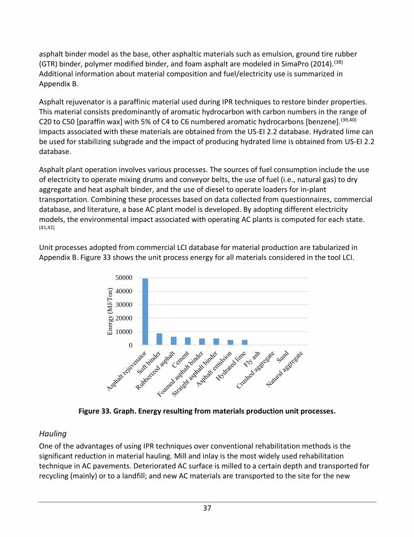
37

asphalt binder model as the base, other asphaltic materials such as emulsion, ground tire rubber (GTR) binder, polymer modified binder, and foam asphalt are modeled in SimaPro (2014).(38) Additional information about material composition and fuel/electricity use is summarized in Appendix B.

Asphalt rejuvenator is a paraffinic material used during IPR techniques to restore binder properties. This material consists predominantly of aromatic hydrocarbon with carbon numbers in the range of C20 to C50 [paraffin wax] with 5% of C4 to C6 numbered aromatic hydrocarbons [benzene].(39,40) Impacts associated with these materials are obtained from the US-EI 2.2 database. Hydrated lime can be used for stabilizing subgrade and the impact of producing hydrated lime is obtained from US-EI 2.2 database.

Asphalt plant operation involves various processes. The sources of fuel consumption include the use of electricity to operate mixing drums and conveyor belts, the use of fuel (i.e., natural gas) to dry aggregate and heat asphalt binder, and the use of diesel to operate loaders for in-plant transportation. Combining these processes based on data collected from questionnaires, commercial database, and literature, a base AC plant model is developed. By adopting different electricity models, the environmental impact associated with operating AC plants is computed for each state. (41,42)

Unit processes adopted from commercial LCI database for material production are tabularized in Appendix B. Figure 33 shows the unit process energy for all materials considered in the tool LCI.

Figure 33. Graph. Energy resulting from materials production unit processes.

Hauling

One of the advantages of using IPR techniques over conventional rehabilitation methods is the significant reduction in material hauling. Mill and inlay is the most widely used rehabilitation technique in AC pavements. Deteriorated AC surface is milled to a certain depth and transported for recycling (mainly) or to a landfill; and new AC materials are transported to the site for the new

0

10000

20000

30000

40000

50000

En

erg

y (M

J/T

on

)

38

surface course. IPR techniques typically do not require much new materials because scarified in situ pavement materials are reused on-site. Hence, material hauling is minimized; this is manifested by capturing environmental benefits when IPR techniques are used.

Environmental Protection Agency (EPA)’s Motor Vehicle Emission Simulator is used to compute the environmental impacts of hauling operations.(43) Based on preliminary simulations, it is found that six parameters, including truck speed, road grade, payload, year, temperature, and relative humidity, affect emissions of heavy truck operations.(44) Through numerous simulations, variable impact transportation (ICT-VIT) model was developed to compute the environmental impacts and energy associated with hauling activities. Types and values of variables considered are summarized in Table 14. The results of preliminary simulations are illustrated in Figure 34 through Figure 37.

Table 14. Types and Ranges of Variables Considered in MOVES Simulations

Figure 34. Graph. Effect of relative humidity on global warming potential (GWP) (T = temperature, RH = relative humidity, G = grade, M = payload).

Figure 35. Graph. Effect of temperature on global warming potential (GWP) (Temp = temperature, RH = relative humidity, G = grade, M = payload).

2.715

2.718

2.721

2.724

2.727

2.730

20 40 60 80 100 120

GW

P (kg C

O2e/tru

ck-m

i)

Relative Humidity (percent)

2.64

2.68

2.72

2.76

2.80

2.84

50 70 90 110 130

GW

P (kg C

O2e/tru

ck-m

i)

Temperature (°F)

Variable Quantity

Vehicle speed (mph) Idling, 1, 2.5, 5, 10, 20, 30, 40, 50, 55, 60, 70

Vehicle weight (tn.sh) 9.07, 15.3, 24.6, 30.1, 33.4, 36.3

Road grade (percent) 0, ±1, ±2, ±3, ±4, ±5, ±6, ±8

Temperature (°F) 0–110

Relative humidity (percent) 30–100

Year 2015–2050

39

Figure 36. Graph. Effect of grade on global warming potential (GWP) (T = temperature, RH = relative humidity, M = payload).

Figure 37. Graph. Effect of payload on global warming potential (GWP) (T = temperature, RH = relative humidity, G = grade).

Construction and Equipment

EPA MOVES 2014 (NONROAD)

The equipment unit processes are compiled using the NONROAD 2008 model incorporated in the MOVES 2014 software. NONROAD equipment are used to perform and help to operate construction activities on-site. Air pollution emission inventories are combined with TRACI impact assessment methodology to estimate the unit emission quantities per gallon of fuel consumed.(45) TRACI 2.1 provides characterization factors for life-cycle impact categories rates: ozone depletion, GWP, acidification, eutrophication, smog formation, human health impacts, ecotoxicity, and fossil fuel depletion for fuel combustion. Figure 38 shows the methodology used to calculate TRACI impact categories rates from eight pollutant types included in MOVES 2014.

0

2

4

6

8

10

12

14

-10 -5 0 5 10

GW

P (kg C

O2e/tru

ck-m

i)Grade (percent)

2.690

2.700

2.710

2.720

2.730

18.1 (full) 9.05 (half full) 0 (empty)

GW

P (kg C

O2e/tru

ck-m

i)

Payload (tn.sh)

40

Figure 38. Chart. TRACI impacts rates calculation from pollutants emissions included in MOVES 2014.

NONROAD Model Development

Simulations have been performed using MOVES 2014 from 2015 to 2050 to allow for running LCIA of equipment for future projects, as shown in Figure 39.

Figure 39. Photo. MOVES 2014 simulations from 2015 to 2050.

41

The simulations run on MOVES 2014 software allowed developing a NONROAD model to assess the environmental impacts of on-site equipment. For a single equipment type, the unit emission of a substance depends on three main variables, which are tier category, HP bin (range), and year of construction. NONROAD model inputs are geographic bound, time spans, NONROAD vehicle equipment type, and pollutants/processes types. The outputs are the rates of the pollutants selected. These rates are then used to calculate the US-EI 2.2 unit processes of diesel combustion. The TRACI characterization of fuel production is used to quantify the unit processes of diesel upstream production. The total per-gallon inventory quantities of diesel combustion and production shares represent the NONROAD equipment impact as illustrated in Figure 40. Figure 41 shows GWP results of equipment types in three counties: Champaign (Illinois), Yolo (California), and Middlesex (New Jersey). The environmental impacts of on-site equipment are not sensitive to geographic location. Because results are not sensitive to location, Champaign County was used to run simulations.

Figure 40. Chart. NONROAD equipment LCI model schematic.

Figure 41. Graph. Sensitivity analysis of equipment GWP results to geographic location.

The model accounts for four tier categories, which are the federal emission standards for compression ignition engines (diesel engines) used in most construction vehicles, resulting from five regulations as follows:

11.69

11.691

11.692

11.693

11.694

11.695

GW

P (

kg

CO

2/g

al)

Champaign

Middlesex

Yolo

42

• “Determination of Significance for Nonroad Sources and Emission Standards for New Nonroad Compression Ignition Engines at or above 37 Kilowatts.”(46) This rule establishes “Tier 1” standards for compression ignition (CI) engines at or above 50 hp (37 kW).

• “Control of Emissions from Nonroad Diesel Engines.”(47) This rule lists “Tier 1” and “Tier 2” standards for CI engines below 50 hp, and “Tier 2” and “Tier 3 “ standards for engines of 50 hp and greater.

• “Control of Emissions from Nonroad Large Spark-Ignition (SI) Engines and Recreational Engines (Marine and Land-Based).”(48) This rule establishes “Tier 2” equivalent standards for recreational marine diesel engines over 50 hp.

• “Control of Emissions from Nonroad Diesel Engines and Fuel.”(49) This rule establishes “Tier 4” standards for CI engines covering all hp categories and regulates diesel fuel sulfur content.

• “Control of Emissions of Air Pollution from Locomotive Engines and Marine Compression Ignition Engines Less Than 30 Liters per Cylinder; Republication.”(50) This rule establishes “Tier 3” standards for recreational marine diesel engines.

The objective of these regulations is to reduce NOx, NMHC, and PM pollutant. Therefore, the impact categories such as smog, acidification, eutrophication, and respiratory effects will decrease over time. Figure 42 shows that respiratory effects impact decreases with the years and with the development of engine technologies through the regulations mentioned above.

Figure 42. Graph. Respiratory effects variation and tier progression of pavers (100<HP<=175) over time.

0

0.005

0.01

0.015

0.02

0.025

0.03

0.035

0.04

Res

pir

ato

ry E

ffec

ts (

CT

Uh/g

al)

Years

T4N

T4

T3

T2

T1

43

Contractors’ data were collected for Tier 2 equipment. Using the NONROAD model, other tier categories were evaluated to compare their impact on the environmental emissions. Using a Tier 4 (T4) instead of Tier 2 (T2) for the CIR single-pass equipment train results in a reduction of 37 of the total respiratory effects as shown in Figure 43.

Figure 43. Graph. Comparison of total respiratory effects of a CIR single-pass equipment train Tier 2 versus Tier 4.

ALLOCATION PROCEDURES

Nicholson showed that environmental impacts and energy resulting from materials production stage is sensitive to the allocation method choice.(52) A 100% cut-off allocation was chosen to manage end-of-life burdens in this LCA study, as illustrated in Figure 44. In fact, pavement construction materials (e.g., AC) may be recycled at the end of life. Therefore, the recycled materials can be either accounted as a burden when using cut-off or as a benefit to the original system using substitution. Figure 45 shows the chain of material life cycle from System 1 (original system) to System 2 (subsequent system).(52)

Figure 44. Chart. Cut-off allocation method system boundary.

0 0.05 0.1 0.15 0.2 0.25 0.3

T2

T4

Total respiratory effects (PM2.5/lane-mile)

Tie

r

Diesel Fuel - 2017 - CIR (single-pass equipment train)

37 percent

44

Figure 45. Chart. Cascade of System 1 and System 2 material life cycles (T = material transportation).

Cut-Off Method

In the cut-off method, the recycling processing R1 is not included in the impacts resulting from system 1 and is considered a burden on System 2. The overall emissions resulting from System 1 material’s life cycle is the summation of emissions due to virgin material input V1 production and hauling, disposal, and hauling of waste to a landfill facility at the end of life of System 1, as Figure 46 shows.

Figure 46. Equation. Cut-off energy/emission calculation formula.

where, X1: proportion of material in the virgin input of System 1

R0: proportion of material in the recycled input of System 0

V1: proportion of material in the virgin input of System 1

W1: proportion of waste material at the end of life of System 1

EV1: emission arising from material in the virgin input of System 1

ER0: emission arising from material in the recycled material of System 0

EW1: emission arising from disposal of waste/landfill material of System 1

45

Substitution (Closed-loop Approximation)

The substitution method gives credit to the original system for producing RAP for the future system as a substitute for virgin materials. The impacts calculation for this method is shown in Figure 47.

Figure 47. Equation. Substitution energy/emission calculation formula.

where R1: is the proportion of material in the product recycled at the end of life of System 1 and ER1 is the emission arising from the material in the recycled input of System 1.

DATA QUALITY ASSESSMENT

Data Quality Requirements

Data quality assessment was conducted following ISO 14044 recommendations and FHWA pavement LCA framework.(1,2,53) High-quality data are important to ensure an accurate LCA study and reliable results to use at the decision-making stage. Table 15 shows the quality goals description assessed in this study.

Table 15. List of Data Quality Requirements

Data Quality Indicator Description

Time-related coverage Age of the data and the minimum length of time over which data should be collected.

Geographical coverage Geographical area from which data or a unit process should be collected to satisfy the goal of study.

Technology coverage Specific technology or technology mix.

Data precision Measure of variability of the data values for each data expressed.

Completeness Percentage of flow that is measured or estimated.

Consistency Qualitative assessment of whether the study methodology is applied uniformly to the various components of the analysis.

The commercial database Ecoinvent and other external software such as MOVES 2014, GREET, and eGRID were used to develop the inventory of upstream and downstream processes. The missing data in materials inventory were addressed by using MSDS. In addition, other processes extracted from an external software are limited to downstream processes such as the emissions compiled using the NONROAD option of MOVES 2014 software. Therefore, appropriate upstream data from Ecoinvent were used to address the missing upstream data.

Data quality was evaluated based on FHWA’s pavement LCA framework and scored based on the greenhouse gas protocol developed by Weidema and Wesneas.(1,53) The score ranges from 1 to 5 to evaluate the reliability of data in life-cycle inventory using the five independent indicators presented in Table 15. The results of data quality assessment are presented in Table 16. Data collection options in Table 16 are defined in the FHWA LCA framework to describe the use of primary and secondary data.(1)

46

Table 16. Data Quality Assessment of Major Modeled Unit Processes

Process Type Unit Process Data Source Data Collection Option Score

Fuel Diesel Public and government databases 4 Fair

Fuel Propane Public and government databases 4 Fair

Electricity Electricity Government and commercial database 4 Good

Construction Equipment MOVES 2014 simulations 4 Good

Hauling Hauling trucks EPA MOVES simulations and commercial database 4 Good

Hauling Single-unit truck EPA MOVES simulations and commercial database 4 Good

Hauling Passenger car EPA MOVES simulations and commercial database 4 Good

Data Validation

The data validation is conducted by comparing the trend of GWP and energy consumption to reveal anomalies in the data. Figure 48 shows that GWP and energy have the same trend as expected, except for cement, where the associated CO2 emissions are the highest among many other materials and that is due to the additional CO2 emissions arising from limestone calcination. Figure 49 and Figure 50 show that the trend for GWP and energy is the same for construction equipment and hauling inventory.

Figure 48. Graph. Data validation of material inventory.

0

200

400

600

800

1000

0

20000

40000

60000

Tota

l G

WP

(k

g C

O2

/Ton

)

Tota

l en

egry

(M

J/to

n)

Total energy (MJ/Ton) Total GWP (kgCO2/Ton)

47

Figure 49. Graph. Data validation of equipment inventory.

Figure 50. Graph. Data validation of hauling inventory.

0

20

40

60

80

100

120

140

160

0

500

1000

1500

2000

2500

Tota

l G

WP

(kg C

O2/g

al)

Tota

l en

ergy

(MJ/

gal

)

Total energy Total GWP

0

1

2

3

4

5

6

-6 -5 -4 -3 -2 -1 0 1 2 3 4 5 6 8

0

0.05

0.1

0.15

0.2

0.25

0.3

0.35

0.4

0.45

Tota

l en

erg

y (M

J/to

n-m

ile)

Grade (percent)

Tota

l G

WP

(k

g C

O2

/ton

-mil

e)

Total GWP - RH = 60 - T = 70 F Total energy - RH = 60 - T = 70 F

48

CHAPTER 5: PAVEMENT PERFORMANCE MODELING

OVERVIEW OF METHODS

Performance and lifetime estimation play a critical role in evaluating life-cycle benefits of in-place recycling treatments as compared with conventional treatments. The methodology to incorporate performance and lifetime estimation into the life-cycle comparative tool is introduced and a two-pronged approach is presented: multi-criteria performance estimation and deterministic performance models. When deterministic models are not available for the selected treatments, a multi-criteria performance estimation approach is proposed to evaluate the selected treatments to make predictions.

• Deterministic performance models—The models in the tool were developed using network-level condition survey data from the California Department of Transportation and are used to predict the international roughness index (IRI) progression and wheel-path cracking performance over the life of pavement. The outputs from these models are estimates of the performance of conventional AC overlays, CIR, and FDR pavements in terms of wheel-path cracking (fatigue cracking) and IRI, which can be used to estimate the time to the next treatment. Similar models can be developed using information from other agencies.

• Multi-criteria performance estimation—This approach utilizes existing information in the literature (e.g., decision-making recommendations from various agencies, treatment lives, guidelines, best practices, expert opinion) to estimate the performance of a treatment considering specific on-site conditions. This approach relies on a process that calculates a “performance score” on a 1 to 5 scale, indicating the level of risk of a selected treatment based on available on-site condition information regarding traffic, climate, existing pavement conditions, soil properties, and material characteristics. The process then compares the performance score with on-site conditions and estimates a treatment life based on the recommendations and other information reported in the literature, which can be modified by the user. This approach also selects an estimated roughness progression rate based on the available information. This approach is used when deterministic performance models do not exist or those available are not considered applicable.

The two approaches determine IRI progression starting from the treatment application time at a trigger IRI value to an IRI threshold value input by the user. This enables the user to visualize the IRI progression and decide the timing of the next treatment. Figure 51 presents the IRI progression for two treatments, A and B, that start, respectively, from 𝐼𝑅𝐼𝑎 and 𝐼𝑅𝐼𝑏 and reach the corresponding thresholds 𝐼𝑅𝐼𝑡ℎ𝑟𝑒𝑠ℎ𝑜𝑙𝑑 .

Both performance-estimation approaches are implemented in the developed tool. Once the project input parameters are entered, the user would be provided with a list of treatment alternatives. The user would have the option to select one or more in-place recycling treatments and compare them to one or more conventional AC overlay treatments. The selected treatments are initially screened for their applicability for the project conditions. If there are obvious and clear barriers against application

49

of the selected treatment (e.g., geometric features impeding application of using a long in-place recycling train), the user would be warned. After this, the user can decide to use either one of the performance modeling approaches to evaluate the selected treatments and calculate treatment lifetime and develop IRI progression curves. In the following schematic (Figure 52), a flowchart of the developed tool illustrates the performance-estimation process integration to the overall flow of data and input flow.

Figure 51. Chart. A schematic of IRI progression curves with significant model parameters obtained by the performance-estimating methods.

Figure 52. Chart. Flowchart of the treatment selection, evaluation, and life-cycle analysis.

50

MULTI-CRITERIA PERFORMANCE ESTIMATION APPROACH

Concept

When there is no performance model available, the multi-criteria performance-estimation approach could be used. The multi-criteria performance-estimation process is used to estimate treatment life by collecting information related to various site-specific conditions and evaluating this information through a rating system to determine an expected treatment performance. This approach provides an estimate of treatment life based on reported lifespans in the literature or observed by the user in the region of interest adjusted for site-specific conditions. The relationship of various site-specific factors to expected performance is compiled from multiple sources. These include existing literature for best practices and experimental data, agency and contractor surveys, decision trees adopted by local and state highway agencies, and expert opinions. A list of bibliographies used in compiling the information required in this process is provided at the end of this document.

The performance estimation process is based on five categories of information: climate, traffic, existing pavement condition, soil properties, and pavement material properties. The process of integrating these into the performance score calculation, treatment suitability, and performance estimation process is as follows:

• Collect site-specific condition information for each major category for a given treatment candidate from the user (traffic, including average daily traffic [ADT]; percent truck and road type; existing pavement condition, including overall condition index and distress level of severity; soil properties; climate type; and materials properties, including mix design if performed).

• Score the site-specific condition under each major category as a risk of poor performance rating score from 1 to 5. The interpretation of each rating score of a treatment under a certain condition is as follows: 1: high risk; 2: medium-high risk; 3: medium risk; 4: medium-low risk; 5: low or no risk.

• For example, a HIR resurfacing treatment followed by a thin overlay of 2 in or less. If a high traffic level of >30,000 AADT is used, a score of 1 is assigned; the literature widely agrees that this treatment type is not suitable for high traffic levels. Assigning a rating of “1” in this case means that there is a high risk that the selected design may perform poorly.

• Evaluate score for each category and determine the final rating score for the application.

• Based on the rating score, calculate expected treatment life based on lifetime estimates compiled from the literature and surveys (see Chapter 4).

The treatment overall performance score (PS) is calculated based on the following formulation (Figure 53). It is assumed that all the factors are independent.

51

Figure 53. Equation. Performance score calculation.

where:

Ti : rating for each traffic related factor i

Ci : rating for each climate condition i

Si : rating for each soil property i

Ei : rating for each existing pavement condition related factor i

Di : rating for material properties condition related factor i

NC : number of climate condition related factors

NT : number of traffic related factors

NS : number of soil properties related factors

NE : number of existing conditions related factors

ND : number of structural design properties related factors

The interpretation of PS and resulting impact on treatment life is explained as follows:

• 4 or 5: Ideal on-site conditions for treatment, indicating very low risk for performance. Treatment life can be expected to be at the highest range.

• 2 or 3: Conditions are fair, carrying a medium risk for the performance of treatment. Treatment life can be expected to be at medium range of expectations.

• 1: On-site conditions are not appropriate for the treatment with very high risk. Treatment life may be predicted at lower range of expected values.

Development of Performance Estimation

Population of the Treatments List

The first step of the development process is to populate a list of anticipated in-place, conventional, and surface treatments. The list of treatments considered in the tool were classified into five categories with their associated expected life range, as shown in Table 17. Table 18 to Table 22 show the expected service life of treatments under each category.(54,55,56) The information reported is based on the literature review and surveys collected from contractors and agencies for IPR treatments application. Agencies’ questionnaire feedback reflects the percentage of agencies that applied various IPR treatments under different life ranges.

52

Table 17. Treatment Categories Expected Life Range

Treatment Category Type Expected Life Range

Category 1 3–5 years





Table 18. Compiled list of Treatment Life Estimates Obtained of Category 1 from Literature Sources

Treatment Type Life Expectancy Range Literature Data Source

Fog seal 1–3 years Peshkin 2011 (54)

Sand seal 3–4 years Peshkin 2011 (54)

Slurry seal 3–6 years Peshkin 2011 (54)

Microsurfacing single course 3–6 years Peshkin 2011 (54)

Chip-seal single course 3–7 years Peshkin 2011 (54)


Treatment Type Life Expectancy Range Literature Data Source Agency Questionnaire Feedback

Cape seal 4–7 years Peshkin 2011 (54) –

Microsurfacing double course 4–7 years Peshkin 2011 (54) –

Chip-seal double course 5–10 years Peshkin 2011 (54) –

HIR resurfacing 6–10 years ARRA 2015 (55) 3–5 years (17%), 5–8 years (50%), 8–10 years (33%)

Thin HMA overlay (2 in or less) 6–12 years Peshkin 2011 (54) –

HIR remixing 3–15 years – 3–5 years (17%), 5–8 years (50%), 8–10 years (33%)


Treatment Type Life Expectancy Range

Literature Data Source

Agency Questionnaire Feedback

CIR 6–10 years ARRA 2015 (54) 1–5 years (7%), 6–10 years (29%), 11–15 years (36%), 16–20 years (21%), >25 years (7%)

CIR + cape seal 6–10 years ARRA 2015 (54) 1–5 years (7%), 6–10 years (29%), 11–15 years (36%), 16-20 years (21%), >25 years (7%)

CIR + chip seal 6–10 years ARRA 2015 (54) 1–5 years (7%), 6–10 years (29%), 11–15 years (36%), 16–20 years (21%), >25 years (7%)

HIR remixing + thin overlay (2 in or less)

7–20 years ARRA 2015 (54) 3–5 years (17%), 5–8 years (50%), 8–10 years (33%)

HIR remixing + medium overlay (between 2 and 4 in)


HIR remixing + thick overlay (over 4 in)


HIR repaving 7–20 years ARRA 2015 (54) 3–5 years (17%), 5–8 years (50%), 8–10 years (33%)

CIR + thin overlay (2 in or less) 7–20 years ARRA 2015 (54) 1–5 years (7%), 6–10 years (29%), 11–15 years (36%), 16–20 years (21%), >25 years (7%)

53





Cold milling + medium overlay (between 2 and 4 in)

6–17 years Peshkin 2004 (56) –

CIR + medium overlay (between 2 and 4 in)

7–20 years ARRA 2015 (55) 1–5 years (7%), 6–10 years (29%), 11–15 years (36%), 16–20 years (21%), >25 years (7%)

FDR 7–10 years ARRA 2015 (55) 6–10 years (8%), 11–15 years (42%), 16–20 years (33%), 21–25 years (8%), >25 years (8%)

FDR +Chip Seal 7–10 years ARRA 2015 (55) 6–10 years (8%), 11–15 years (42%), 16–20 years (33%), 21–25 years (8%), >25 years (8%)

FDR +Cape Seal 7–10 years ARRA 2015 (55) 6–10 years (8%), 11–15 years (42%), 16–20 years (33%), 21–25 years (8%), >25 years (8%)





CIR + thick overlay (over 4 in) 7–20 years ARRA 2015 (55) 6–10 years (8%), 11–15 years (42%), 16–20 years (33%), 21–25 years (8%), >25 years (8%)

Cold milling + thick overlay (over 4 in)

17–30 years Peshkin 2004 (56) 6–10 years (8%), 11–15 years (42%), 16–20 years (33%), 21–25 years (8%), >25 years (8%)

FDR + thin overlay (2 in or less)

More than 20 years

ARRA 2015 (55) 6–10 years (8%), 11–15 years (42%), 16–20 years (33%), 21–25 years (8%), >25 years (8%)

FDR + medium overlay (between 2 and 4 in)

More than 20 years


FDR + thick overlay (over 4 in) More than 20 years


Performance Estimation Process and Integration to the Tool

The information provided by the user under five criteria categories are used to assess the performance of any treatment selected by the user. This section introduces the major criteria categories and the information requested specifically by the user. The traffic and soil properties inputs are used to generate the pavement design candidates that meet the required structural capacity. The five major criteria are as follows:

• Traffic: The criteria to be evaluated under this category include traffic level (AADT or/and ESALs), truck volume (percent), and road type (urban, rural). Traffic conditions are used to evaluate suitability of different treatments. For example, treatments such as CIR are generally used and recommended for lower volume roads whereas FDR can be designed to serve adequately for higher volume roads.

• Existing pavement conditions: This category is evaluated by criteria related to drainage adequacy, ride quality, and either overall pavement condition index or composition of critical distresses present in the pavement. The existing conditions of a pavement are vital for

54

evaluating the relevance of treatment types. For example, the severity and type of distresses may limit the usefulness of some treatments (e.g., HIR surface recycling), which cannot address structural distresses.

• Soil properties: Characterization of the structure and soil type helps in determining which designs are more likely to satisfy structural capacity requirements. The user is asked to input a value of the California bearing ratio (CBR) to evaluate the support of pavement. This input is also used in the pavement design criteria that is introduced later.

• Material properties: The tool evaluates mix designs as part of this approach, if provided. It is assumed that the use of a mix design reduces risks and accounts for the use of additives and their dosages that affect pavement performance.

• Climate: The climate may have an impact on the performance of some treatments. Normally, one should expect that the designs should be adjusted according to the climate conditions. However, there may be some treatments performing favorably under certain climatic conditions such as micro-surfacing under warmer climates.(4) Another factor is the curing time required when additives are used along with in-place recycling techniques. Therefore, the different climate conditions considered in this study are cold/wet, cold/dry, hot/dry, and hot/wet.

The overall performance score value defines the risk factor that should be applied on the treatment. This process is applied on all the treatments selected by the user and directly influences treatment life expectancy. The major category criteria are scored for each treatment considered in the tool using previous studies (e.g., Peshkin 2011 and ARRA 2015; Stroup-Gardiner 2011; IDOT 2012; Wu et al. 2010; Hicks et al. 1999) where decision matrices were developed to help in decision-making at the network level.(4,54,55,57,58,59) Appendix C shows the “IPR Decision Matrix” for rehabilitation and preservation treatments selection and evaluation matrix.

Some limitations of this approach include the fact that rating of on-site conditions classified under five categories relies on information available in the literature and expert opinion without supporting data. Therefore, a validation step was conducted to support the design lives estimated by this approach. The validation step includes case studies (Appendix F) with performance data available and vetting by internal and external experts. Case studies were chosen primarily from the following sources:

• Local and state highway pavement management databases (CalTrans, IDOT, and others).

• LCA studies conducted to assess the environmental impacts and to evaluate the performance of preventive maintenance treatments.

• An INDOT study that show models to measure short- and long-term effectiveness of highway pavement maintenance.

55

The approach described in this chapter is applied to score the selected treatments, and the estimated treatment life is compared to the ones observed in these case studies (Appendix F). The performance scoring criteria can be fine-tuned based on this step to improve accuracy.

Table 23 shows the five criteria categories and conditions considered under each category in the decision matrix. The selected treatment score points range from 1 to 5 for each one of these conditions. These values are used to assess the treatments’ overall performance.

Table 23. List of Main Components of the Performance Evaluation Categories

Criteria Category Conditions (Subcategories) Possible Values/Ranges

Traffic Traffic level (AADT and/or ESALs) Low, Medium, High

Traffic Percent truck volume <10 percent or >=10 percent

Traffic Road type Rural, Urban

Existing pavement conditions PCI or an Equivalent Overall Condition Index Good, Satisfactory, Fair, Poor

Existing pavement conditions Raveling Low, Medium, High

Existing pavement conditions Potholes Low, Medium, High

Existing pavement conditions Bleeding Yes/No

Existing pavement conditions Low Skid Resistance Yes/No

Existing pavement conditions Shoulder Drop-Off Yes/No

Existing pavement conditions Rutting-Wear Low, Medium, High

Existing pavement conditions Corrugations Low, Medium, High

Existing pavement conditions Shoving Low, Medium, High

Existing pavement conditions Fatigue Cracking Low, Medium, High

Existing pavement conditions Edge Cracking Low, Medium, High

Existing pavement conditions Slippage Low, Medium, High

Existing pavement conditions Block Cracking Low, Medium, High

Existing pavement conditions Longitudinal Cracking Low, Medium, High

Existing pavement conditions Transverse Cracking Low, Medium, High

Existing pavement conditions Rough Ride Quality Yes/No

Existing pavement conditions Drainage Adequacy Yes/No

Soil properties CBR Good (CBR >=10), Fair (3<CBR<10), Poor (CBR>=3)

Structural design Pavement design performed Yes/No

Climate Type Dry/Cold (−20ºF/14ºF), Wet/Cold (14ºF–50ºF), Wet/Hot (50ºF/64ºF), Dry/Hot (>64ºF)

Example: Case Study

Suppose the user selects CIR with a thin HMA overlay and inputs the criteria in Table 24.

56

Table 24. Example of PS Criteria

Criteria category Conditions Possible values/ranges PS

Traffic Traffic level AADT 40,000 1

Traffic Percent Truck Volume 20% 1

Traffic Road type Rural 5

Existing pavement conditions PCI Good 5

Existing pavement conditions Raveling High 5

Existing pavement conditions Potholes Low 5

Existing pavement conditions Bleeding Yes 3

Existing pavement conditions Skid Resistance Low 5

Existing pavement conditions Shoulder Drop-off No 5

Existing pavement conditions Rutting-Wear Low 4

Existing pavement conditions Corrugations High 5

Existing pavement conditions Fatigue cracking Low 5

Existing pavement conditions Edge cracking Low 5

Existing pavement conditions Slippage Medium 4

Existing pavement conditions Block cracking Low 5

Existing pavement conditions Longitudinal cracking Low 5

Existing pavement conditions Transverse cracking Low 3

Existing pavement conditions Rough ride quality Yes 5

Existing pavement conditions Drainage adequacy Yes 5

Soil properties CBR (percent) 7 1

Structural design Pavement design performed Yes 5

Climate Climate condition Wet/Hot 5

In the performance score calculation, the rating of existing pavement conditions is either calculated through PCI or by considering the average of rating scores of all structural and non-structural distresses. This distinction is because the PCI calculation considers the extent of distresses and level of severity. Therefore, if PCI is considered in the existing pavement condition evaluation, PS would be equal to 3, as shown in Figure 54, which comprises the rating for traffic conditions, PCI, soil properties, material properties, and climate type.

Figure 54. Equation. PS calculation using PCI.

Otherwise, if the rating of the different distresses is considered, then PS calculation is shown in Figure 55.

Figure 55. Equation. PS calculation using distress survey.

57

The conditions are fair, indicating medium risk for the performance of the treatment.(55) Treatment life can be expected to be at medium range of expectations, which is 6 to 10 years.

Implementation in the Tool

First, the tool applies the multi-criteria performance-estimation approach so that the risk level of the treatments can be evaluated through the performance score calculation. Second, it calculates life expectancy of the treatments using either deterministic performance models or the multi-criteria approach estimation in case no performance model is available for the user selections. The deterministic or mechanistic performance models are viewed as the best approach for predicting pavement performance and checking the multi-criteria performance-estimation approach.

The tool is flexible enough that users can implement their own performance models by inserting their model coefficients or modify the expected range of treatment lifetime based on their regional experiences. Once the life expectancy of the selected treatments is decided, the timeline of future maintenance and rehabilitation activities for the pavement is estimated and the environmental impacts over the estimated life of the pavement are calculated by the LCA engine of the tool.

DETERMINISTIC PERFORMANCE MODELS

Introduction

Environmental impacts of the pavement-use stage considered in this study are due to (1) excess fuel consumption (EFC) of vehicles traveling on the section in the use stage and (2) maintenance and rehabilitation (M&R) activities, including the initial IPR or reclamation treatment, that are applied to the pavement to restore structural capacity and ensure safety and serviceability.

EFC is defined as the fuel used beyond what is needed to travel on an “ideal” pavement, i.e., smooth pavement with no more macrotexture than what is needed to provide safe friction and having no fuel consumption due to the structural response of the pavement. Of these three mechanisms (roughness, texture, and structure) causing EFC, surface roughness, as measured by the IRI, is the mechanism affecting vehicle fuel economy considered in this study. This study considers IPR or reclamation of asphalt pavements and compares the effects on energy consumption of using these treatments with asphalt overlays. The other two mechanisms are not considered. Differences in macrotexture and structural response are assumed to be very minimal between the recycling and reclamation strategies and the overlays, while development of roughness is assumed to be different enough to warrant consideration. To estimate excess vehicle fuel consumption, models are needed to predict surface roughness with time and truck traffic. These models are then coupled with vehicle-pavement interaction (PVI) models to translate pavement roughness into EFC.

Agencies normally use decision trees to determine the frequency of future M&R activities based on comparison of pavement condition indices with threshold values for those indices to trigger M&R activities. These decision trees are usually based on perception of optimality for cost effectiveness of the timing of the treatment and previous experience in managing their network and are implemented subject to budget availabilities.

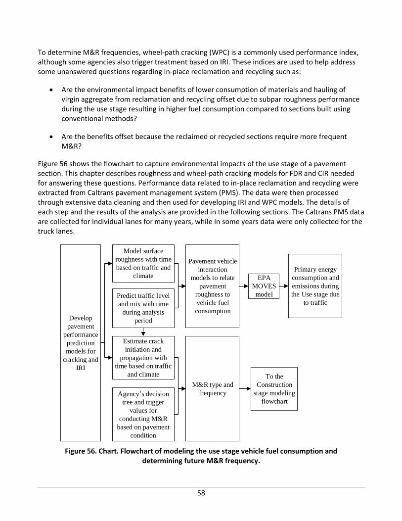
58

To determine M&R frequencies, wheel-path cracking (WPC) is a commonly used performance index, although some agencies also trigger treatment based on IRI. These indices are used to help address some unanswered questions regarding in-place reclamation and recycling such as:

• Are the environmental impact benefits of lower consumption of materials and hauling of virgin aggregate from reclamation and recycling offset due to subpar roughness performance during the use stage resulting in higher fuel consumption compared to sections built using conventional methods?

• Are the benefits offset because the reclaimed or recycled sections require more frequent M&R?

Figure 56 shows the flowchart to capture environmental impacts of the use stage of a pavement section. This chapter describes roughness and wheel-path cracking models for FDR and CIR needed for answering these questions. Performance data related to in-place reclamation and recycling were extracted from Caltrans pavement management system (PMS). The data were then processed through extensive data cleaning and then used for developing IRI and WPC models. The details of each step and the results of the analysis are provided in the following sections. The Caltrans PMS data are collected for individual lanes for many years, while in some years data were only collected for the truck lanes.

Develop

pavement

performance

prediction

models for

cracking and

IRI

EPA

MOVES

model

Primary energy

consumption and

emissions during

the Use stage due

to trafficPredict traffic level

and mix with time

during analysis

period

Model surface

roughness with time

based on traffic and

climate

Estimate crack

initiation and

propagation with

time based on traffic

and climate

Pavement vehicle

interaction

models to relate

pavement

roughness to

vehicle fuel

consumption

Agency s decision

tree and trigger

values for

conducting M&R

based on pavement

condition

M&R type and

frequency

To the

Construction

stage modeling

flowchart

Figure 56. Chart. Flowchart of modeling the use stage vehicle fuel consumption and determining future M&R frequency.

59

Data Collection

Initial Data Analysis and Characterization

Caltrans PMS condition survey database, consisting of the previously used visual pavement condition survey (PCS) and the automated pavement condition survey (APCS) began in 2011, was used to collect data for sections that have had CIR or FDR at any point in their service life. The entire process of data collection, data cleaning, and model development was conducted two times. In the first attempt, close to 2.7 million observations were collected for all CIR and FDR sections using the PCS as well as 2011 and 2012 APCS data. As the 2015 APCS data became available (there were no surveys in 2013 and 2014), a second attempt was carried out to see if the models could be improved by using updated data and implementing the experience gained from running the entire process in the first attempt. Separate data frames were extracted for CIR and FDR in the second attempt. The process of data extraction consisted of the following steps:

• Identification of the 32.6 ft (10 m) long data collection segments in the network, identified by “section IDs,” that had CIR/FDR at any points in their history.

• Extraction of all the observations for those IDs from the database.

This method was used to capture the full-time history of the development of cracking and IRI on the sections that had CIR/FDR, not just the observations immediately after the CIR/FDR execution and just before the next major treatment. Table 25 shows a general categorization of the collected data.

Table 26 summarizes the database before data cleaning. The information in these tables is obtained from the second round of data collection from Caltrans PMS database in which separate data frames were extracted for CIR and FDR. There were two types of FDR in the collected data, FDR with no stabilization (FDR-NA) and FDR with foamed asphalt (FDR-FA). Table 27 shows the number of observations for each climate region.

Table 25. General Categorization of the Data Available in the Database

General Section Information

Project Contract Information (as-built)

Project Construction Activities Condition Survey Data of the Sections

Route Expenditure authorization (EA) **

Information about the previous layers that were in place

Date of condition survey

Direction LOC of a project *** Number and thickness of the removed layers

IRI in the left and right wheel paths

Beginning and ending odometer

Project award date Type of applied treatments

Fatigue cracking in the wheel path (called alligator cracking) classified into three levels of severity: A (initial unconnected cracks), B (progression to intersecting cracks), and C (intersecting cracks extending between wheel paths)

Length Project completion date

Number and type of the layers that were added /recycled in place

Other performance indices (such as bleeding, patching, rutting, …) ****

60

General Section Information

Project Contract Information (as-built)

Project Construction Activities Condition Survey Data of the Sections

Lane - - -

Climate - - -

Unique ID for each sub-section

- - -

Traffic levels (ESALS* per year)

- - -

* Equivalent Single Axle Load

** EA is the funding source used for conducting the project. Multiple projects in various locations can have the same EA.

*** LOC is not an acronym, just a term used in Caltrans’ PMS. Each LOC number refers to a specific treatment (in terms of structural and mix design, and construction activities), and it has nothing to do with the project location. A single LOC could have been implemented in multiple locations.

**** These indexes were not directly used in this study but helped clarify the history of sections during data cleaning.

Table 26. Summary of the Databases Extracted for CIR and FDR from Caltrans PMS

Data Information CIR FDR

Number of Observations ([# of obs.] data segments times survey years with observations)

416,952 433,925

ID 12,367 15,918

LOC 509 1,025

EA 377 777

Climate regions (out of nine in state) 7 9

Table 27. Distribution of Observations across Climate Regions

Climate (CIR) # of obs. Climate (FDR) # of obs.

Inland Valley 143,181 Inland Valley 120,393

High Desert 91,712 Low Mountain 90,229

Desert 70,200 High Mountain 53,838

High Mountain 60,711 South Coast 46,761

Low Mountain 35,975 High Desert 45,367

South Coast 13,796 Central Coast 26,703

Central Coast 1,377 Desert 25,991

– – North Coast 19,965

– – South Mountain 4,678

Data Cleaning

Figure 57 was used as the framework for conducting data cleaning.

61

Identify the LOCs that

have in-place recycling

in their construction

history.

Use the selected

observations for model

development.

For each LOCi, identify all unique IDs

associated with it, then search the whole

database for those IDs and assign:

LOC_Corr = LOCi

This is done to capture the complete history of

each ID, as multiple LOCs could have been

applied on the same ID.

Example each plot and identify observations

that are reasonable:

• IRI and cracking levels are expected to

drop after a treatment is applied

• IRI and cracking values are expected to

increase with time

• Fix construction end date where needed

• This has to be done separately for the

IRI and cracking plots.

• Selected LOC_Corr s with more than

one sample date

• Plot the IRI and wheelpath cracking for

each

• Highlight the project award and

completion dates for each of the actual

LOCs as one ID can have multiple

LOCs (CIR/FDR dates in red and the

rest in blue).

Figure 57. Chart. Flowchart for conducting data cleaning.

The third stage of the flowchart above resulted in:

• CIR: 120 unique LOCs were identified for IRI and 114 for WPC.

• FDR: 309 unique LOCs for IRI and 278 for WPC.

Figure 58 shows a sample of the scatter plots and box plots for the time histories of observations on sub-segments (section IDs) of roughness and wheel-path cracking developed for each LOC to evaluate the reasonableness of the data versus the as-built history.

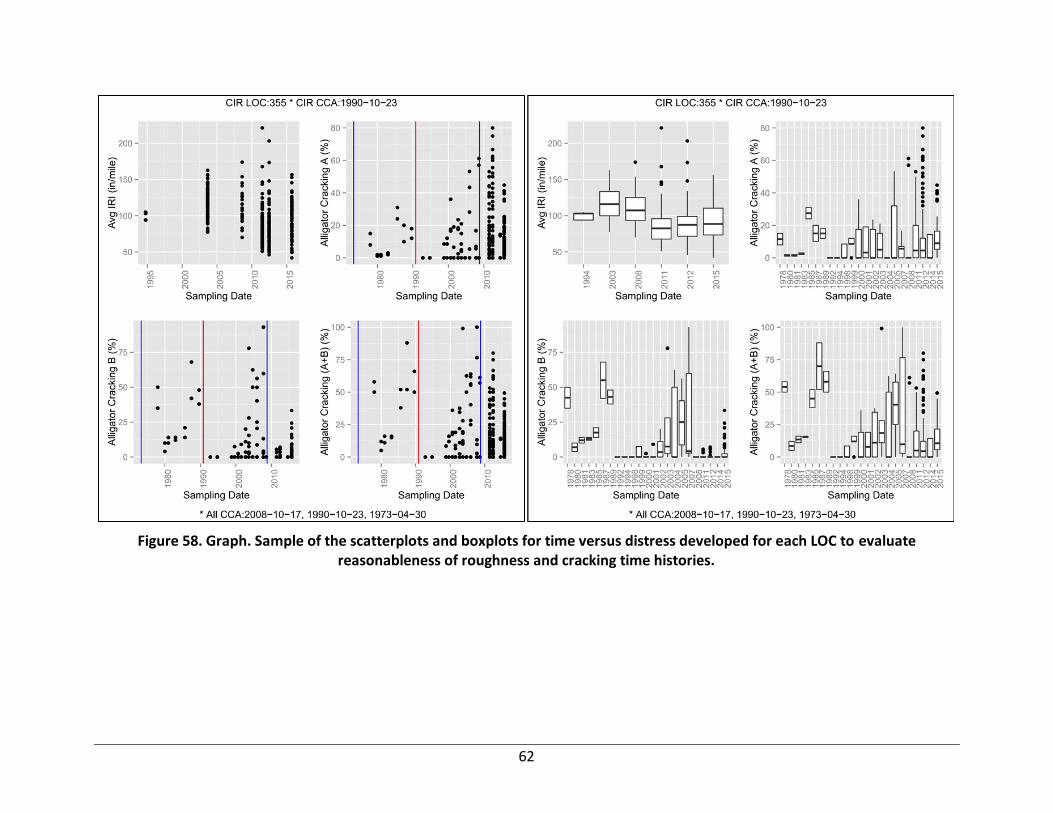
62

Figure 58. Graph. Sample of the scatterplots and boxplots for time versus distress developed for each LOC to evaluate reasonableness of roughness and cracking time histories.

63

The last step was to manually review the plot and its supporting data for each LOC and determine whether the observed trend is reasonable and if the data are useful for developing performance models. There were cases of unexpected decrease in IRI or cracking and no record of any maintenance or rehabilitation. This might be because documentation of construction activities was not perfect in the PMS database and, therefore, parts of a section history of treatment were lost. In other cases, the high values of IRI recorded were inconsistent with the trend before or after that specific date of sampling. This indicates the possibility of measurement error in that particular survey. Furthermore, there were cases where the trends of progression of IRI and cracking were consistent with what was expected but the reduction in IRI and/or cracking, expected to happen after the treatment, did not match the dates recorded for construction completion. These were likely due to errors in recording project completion dates. The number of observations in the datasets after data cleaning is shown in Table 28.

Table 28. Summary of the Data Frames after Data Cleaning

Data Information IRI-CIR IRI-FDR WPC-CIR WPC-FDR

Total Observations 29,229 35368 19,311 23,090

ID 8,645 6284 8,073 7,827

LOC 83 206 75 130

EA 126 100 63 143

Climate Region 6 9 7 9

Performance Modeling

Introduction

As explained at the beginning of this chapter, two performance variables were selected for this project: IRI and WPC. The performance variable for IRI was defined as the IRI values measure for each of the section IDs. Each ID has a length of 0.1 mi, and the average value of IRI reading on that section is reported as the IRI for that ID.

The modeling processes for IRI and WPC are both empirical-mechanistic, meaning that the variables included in the model and the equation form of the model are predetermined based on the behavior expected from mechanistic analysis, but they are empirical, meaning that there are no mechanics calculations performed. The performance models for conventional treatments in continuous form are shown in Table 29. The WPC model consists of crack initiation and crack progression. Using a performance tree was deemed beneficial to facilitate combining these two models into one continuous form to be implemented in the final tool delivered by this project.

To use climate as a categorical variable and to have enough observations for each climate category, it was assumed that climate regions can be categorized as severe or mild. Table 30 shows the classification of climatic regions into mild and severe climate based on average annual rainfall. Table 32 and Table 33 show the categories considered for the traffic level and overlay thickness, respectively. Overlay thickness was considered as the total added thickness in the modeling section, which represents the total thickness of layers added on top of the FDR or CIR. The same AC thickness overlay categories were used for the surfaces placed in CIR and FDR treatments and for AC overlays

64

without CIR and FDR. Figure 59 is a representation of one of the performance tree branches. Each branch has its own performance model coefficients (where data availability and data quality permit) as indicated in Tseng.(60) Models for AC overlay without CIR or FDR used in this project were those developed previously for the Caltrans PMS.

Table 29. Performance Equations Used for AC Models without CIR or FDR Developed by Tseng

Performance Variable

Intended Purpose Pavement Condition Index Used

Performance Equation Form

International Roughness Index

IRI is an indicator of surface roughness.

IRI

Wheel-path Cracking

WPC is caused by aging and traffic load and is used as an indicator of the structural capacity of pavement sections and therefore a metric for triggering rehabilitation.

Percent of wheel path with crack length ratio greater than 1.6 (when cracks are specified as Alligator B by Caltrans)

𝑦 = 100 ∗ (1 − 𝑒(−𝑥𝑎)𝑏

)

Table 30. Classification of Severe Climatic Regions

Severe Climate Annual Rainfall (inch)

North Coast 41.9

High Desert 7.5

High Mountain 21.4

South Mountain 34.2

Low Mountain 32.6

Table 31. Classification of Mild Climatic Regions

Mild Climate Annual Rainfall (inch)

Inland Valley 17.7

Central Coast 21.3

Desert 3.9

South Coast 13.0

Table 32. Traffic Categories Considered for the Performance Tree

Traffic Levels ESALs/Lane/Year

Low (A) Less than 100,000

Medium (B) 100,000 to 500,000

High (C) More than 500,000

Table 33. Asphalt Concrete Surface Thickness Categories Considered for the Performance Tree

Overlay Thickness

Thin Less than 0.2 ft

Medium 0.2 to 0.5 ft

Thick More than 0.5 ft

65

Figure 59. Chart. Representation of one of the performance model tree branches.

Cracking Models

The modeling of WPC is different from IRI, as cracking is often a latent variable, which means that even though it exists, it is not observed until it reaches the surface. Structural deterioration of the pavement starts right after construction and is continuous under traffic load and climate impacts. As the pavement deteriorates, cracks start to form in the AC layer; however, these cracks may not appear in some cases on the pavement surface for a considerable amount of time. Even when cracking begins at the top of the AC layer, it takes some time for the cracks to become wide enough to be measurable. This is not the case for surface roughness, as it can be measured immediately after construction and a singular continuous model could be used for predicting future IRI values. Therefore, the WPC models developed under this study consist of two separate stages: models for determining the time to crack initiation (first cracks appearing on the surface) and models for predicting the propagation of additional cracks with time.

The method adopted for performance modeling was implemented in earlier efforts for developing WPC models for conventional treatments such as AC overlays and seal coats.(60,61,62,63) Data collected in this study for the sections built using IPR represent time series observations of separate pavement sections, referred to as “panel data.” These sections have different traffic levels, climate conditions, and overlay thicknesses. To develop models considering each section having random effects, mixed-effect models were used in developing WPC models.

WPC is measured separately for the right and left wheel path by Caltrans and is quantified in terms of wheel-path crack length ratio, RWPC, which is the ratio of total length of all wheel-path cracks to the length of data segment.(64) WPC ratios of up to 1.6 are considered as Alligator A cracking and above that as Alligator B. Alligator C is the final form of fatigue cracking when the fatigue cracks between right and left wheel paths connect. The performance variable for WPC in this study was defined as percent of the wheel path length with Alligator B cracking. The collected dataset from Caltrans PMS database report cracking in terms of percent of each section with Alligator A cracking and the percent of each section with Alligator B. Average values of Alligator B WPC for the right and left wheel path were used for this study.

Crack initiation time was defined as the lower value of these two times after initial construction: (1) 5% of the section has Alligator A cracking, or (2) Alligator B cracking is greater than zero on the

Type of In-place Recycling

CIR

Mild Climate

Low Traffic

Thin Overlay

Medium Overlay

Thick OverlayMedium Traffic

High TrafficSevere Climate

FDR

66

section. Survival analysis was used for estimating crack initiation time. It was assumed that crack initiation occurs at 50% survival probability. The survival curves for CIR and FDR at different traffic levels are presented in Figure 60 and Figure 61, and the results of survival analysis are presented in Table 35 and Table 36. The survival curve for high traffic level in Figure 60 is expected to fail sooner than the other two categories of traffic, which is not observed. This is due to the lack of data for this section of analysis as CIR was not used for high traffic sections, as shown in the results in Figure 60 obtained from Stata software. (65)

Table 34. Survival Analysis Results for FDR Sections

ESALs Time at Risk Incidence Rate

No. of Subjects

Survival Time: 25%

Survival Time: 50%

Survival Time: 75%

High 26189705 0.0000240 16,185 1734 2860 3421

Low 2783149174 0.0001449 1,357,876 2378 3580 5926

Med 500862801 0.0002010 281,799 2185 2791 3766

Total 3310201680 0.0001541 1,655,860 2378 3400 4862

Figure 60. Photo. Survival curve for CIR sections. The legend refers to traffic levels.)

Table 35. Survival Analysis Results for CIR Sections

ESALs Time at Risk Incidence Rate No. of Subjects

Survival Time: 25%

Survival Time: 50%

Survival Time: 75%

High 78926208 0.0000148 57,441 – – –

Low 432091198 0.0001554 291,514 2330 3595 4697

Med 49575317 0.0001791 36,738 2658 2791 4359

Total 560592723 0.0001377 385,693 2585 3595 4697

0.0

00.2

50.5

00.7

51.0

0

0 2000 4000 6000 8000analysis time

High Low

Med

Kaplan-Meier survival estimates

67

Figure 61. Photo. Survival curve for FDR sections. (The legend refers to traffic level.)

Table 36. Survival Analysis Results for FDR Sections

ESALs Time at Risk Incidence Rate

No. of Subjects Survival Time: 25%

Survival Time: 50%

Survival Time: 75%

High 26189705 0.0000240 16,185 1734 2860 3421

Low 2783149174 0.0001449 1,357,876 2378 3580 5926

Med 500862801 0.0002010 281,799 2185 2791 3766

Total 3310201680 0.0001541 1,655,860 2378 3400 4862

As stated earlier, WPC cracking is a latent variable. Therefore, possible data censorship, due to not knowing the value of WPC in places where it has not reached the surface yet, need to be accounted for. Thus, an incidental truncation term, lambda (λ), was added to the crack progression stage. This correction term was added to address the possibility of the latent variable, WPC, to be positive without being observed or measured. λ represents the possibility of crack initiation. To estimate λ, an ordered probit model was used assuming WPC to have three possible conditions: no cracking, Alligator A, or Alligator B. Details of statistical assumptions and theories for selection of modeling approaches are presented elsewhere.(60,61,62,63)

Mixed-effect logit models were used for crack progression because the data must be fitted into a predefined exponential function form. The initial equation form and the transformations needed to change the equation into a linear form so that the mixed-effect linear regression could be correctly used are presented in Figure 62. Various combinations of possible explanatory variables were tested to determine the best possible model that has the highest accuracy and follow the expected trends (such as positive coefficient for the age variable). Explanatory variables included λ, climate (a

0.0

00.2

50.5

00.7

51.0

0

0 2000 4000 6000 8000 10000analysis time

High Low

Med

Kaplan-Meier survival estimates

68

categorical variable represented by 1 for severe and 0 for mild), overlay thickness (in mm), traffic level (in ESALs), and previous Alligator B extent before treatment.

Figure 62. Equation. Transformation applied to the original equation for WPCs.

The right-hand expression in the final equation in Figure 62 is considered as z. Mixed-effect linear regression models were tested on z versus ln(age). To account for other explanatory variables (EVs), different combinations were considered in the iterations. To develop a model with age as the only EV, these variables were considered in combination with ln(age). This considered the impact of each significant EV. Assuming a crack initiation time of t0, crack initiation and progression can be combined as shown in Figure 63.

Table 37 and Table 38 show the selected model for the CIR sections. As the results show, age, λ, traffic level, and overlay thickness were significant factors affecting CIR sections’ performance. Previous Alligator B level and climate region were found to be insignificant. Table 39 and Table 40 present the selected model for FDR sections. Traffic level, previous Alligator B, and climate condition were found to be insignificant factors, while λ is significant.

Figure 63. Equation. Combination of crack initiation and progression models.

69

To combine crack initiation and propagation, the progression curve begins at the point where crack initiates (predicted age). Figure 64 and Figure 65 show the performance curves for CIR and FDR. For crack initiation, CIR performs similarly to FDR, but CIR sections deteriorate relatively rapidly after crack initiation, while FDR sections show a relatively slower crack propagation. As expected, the sections with higher traffic level have a higher rate of deterioration. For the same level of traffic, thicker overlay reduces the rate of cracking. Exceptions were noted for CIR: (1) medium overlay performed worse than thick overlay for traffic level B and (2) thick overlay with traffic level B performed worse than thick overlay with traffic level C. FDR performance was as expected too, except for two cases: (1) thin overlay performed better than medium overlay for traffic level B and (2) thin overlay shows worse performance compared with medium and thick overlays for traffic level A. These cases are under further investigation to fix for the identified issues.

Table 37. Descriptive Statistics of Final WPC Model for CIR, with Confidence Intervals and Significance Level of Parameters

z Coefficient Std. Err. z P>|x| 95% CI Lower Limit 95% CI Higher Limit

“lnage” 1.797321 0.062065 28.96 0.000 1.67574 1.91896

“lambdalnage” 0.573032 0.024017 23.95 0.000 0.52823 0.62237

“lnesalslnage” 0.078876 0.005549 14.21 0.000 0.06799 0.08975

“total_added_thicknesslnage” -0.002343 0.000289 -8.08 0.000 -0.00291 -0.00175

cons -21.08975 0.400718 -52.63 0.000 -21.87515 -20.30436

Table 38. Descriptive Statistics of Random Effects Parameters of Final WPC Model for CIR

Random Effects Parameters

Estimate Std. Err. 95% CI Lower Limit 95% CI Higher Limit

sd(cons) 1.42266 0.05548 1.31797 1.53566

sd(Residuals) 0.78187 0.00203 0.77801 0.78851

Table 39. Descriptive Statistics of Final WPC Model for FDR, with Confidence Intervals and Significance Level of the Parameters

z Coef. Std. Err. z P>|x| 95% CI Lower Limit

95% CI Higher Limit

“lnage” 1.159264 0.0070786 163.77 0.000 1.14539 1.173138

“lambdalnage” 0.6306005 0.0034349 183.59 0.000 0.6238682 0.6373327

“total_added_thicknesslnage”

-0.0003864 0.0000434 -8.89 0.000 -0.0004716 -0.0003013

cons -13.08842 0.0524070 -249.75 0.000 -13.19113 -12.9857

Table 40. Descriptive Statistics of Random Effects Parameters of Final WPC Model for FDR

Random Effects Parameters Estimate Std. Err. 95% CI Lower Limit 95% CI Higher Limit

sd(cons) 1.51566 0.01775 1.48126 1.55087

sd(Residuals) 0.702703 0.00070 0.70132 0.70408

70

Figure 64. Graph. Crack initiation and progression models combined for CIR section (A, B, C refer to low, medium, and high traffic levels).

Figure 65. Graph. Crack initiation and progression models combined for FDR section (A, B, C refer to low, medium, and high traffic levels).

Roughness Models

The cleaned data frames were used for derivation of IRI models for CIR and FDR. As the analysis consists of cross-sectional data of pavement network over time (panel data), mixed-effect linear regression was selected, and Stata software was used for model development.

0

20

40

60

80

100

0 5 10 15 20 25 30

Percen

t of

Secti

on

s w

ith

All

igato

r B

Age(years)

Crack Initiation and Progression

A, Thin

A, Med

A, Thick

B, Thin

B, Med

B, Thick

C, Thin

C, Med

C, Thick

0

20

40

60

80

100

0 5 10 15 20 25 30

Percen

t of

Secti

on

s w

ith

All

iga

tor B

Age(years)

Crack Initiation and Progression

A, Thin

A, Med

A, Thick

B, Thin

B, Med

B, Thick

C, Thin

C, Med

C, Thick

71

The first step was to check the significance in IRI difference before and after treatment. Student unpaired t-test was used and showed that CIR treatments significantly reduced IRI, with an average IRI reduction of 78 in/mi. The same procedure was performed for the FDR sections and the results showed that FDR resulted in an average reduction of 91 in/mi. Average IRI after construction for CIR section was 90 in/mi, for FDR with no stabilization was 92 in/mi, and for FDR with foamed asphalt stabilization was 72.5; the standard deviations were 3.7, 3.3, and 5.7, respectively.

Similar to the iterations explained in modeling the WPC, various combinations of EVs were tested to select the most appropriate model based on significance of EVs in the model and the model accuracy in minimizing errors. For both CIR and FDR, average IRI (iri_avg) was regressed as the dependent variable versus multiple combinations of age, ESAL/lane/year, previous IRI, and climate as independent (explanatory) variables. Natural logarithm transforms of the EVs were also tested to identify the best model. The analysis was weighted based on the length of subsections. Table 41 to Table 49 show the results for CIR, FDR with no stabilization and FDR with foamed asphalt. The models for each treatment are shown Figure 66 to Figure 68 and are also summarized in Table 50.

Table 41. IRI Performance Model for CIR

iri_avg Coef. Std. Err. z P>|x| 95% CI Lower Limit

age -0.003304 0.000212 -15.6 0.000 -0.00372

agelnesals 0.008695 0.000018 49.91 0.000 0.00086

agesevere 0.004013 0.000091 44.08 0.000 0.00383

agethick -3.52E-06 7E-07 -5.21 0.000 -4.85E-06

cons 90.447512 3.707305 24.4 0.000 83.18133

Table 42. Descriptive Statistics of Random Effects Parameters of IRI Performance Model for CIR

Random Effects Parameters

Estimate Std. Err. 95% CI Lower Limit 95% CI Higher Limit

sd(cons) 38.16008 2.63411 33.33132 43.68840

sd(Residuals) 18.42575 0.02048 18.38564 18.46595

Table 43. Statistical Parameters of IRI Performance Model

Parameter Value

Log Likelihood -1753438.4

Number of observations 404,588

Number of groups 106

Obs. per group: min 12

Obs. per group: avg 3816.9

Obs. per group: max 23,926

Wald chi2(4) 39329.58

prob>chi2 = 0.0000

72

Figure 66. Equation. Performance model for IRI progression of CIR sections.

Table 44. IRI Performance Model for FDR with No Stabilization

iri_avg Coef. Std. Err. z P>|x| 95% CI Lower Limit 95% CI Higher Limit

age 0.001398 0.00065 2.13 0.033 0.00011 0.00268

agelnesals 0.000620 0.00006 10.53 0.000 0.00050 0.00074

cons 92.49978 3.349089 27.62 0.000 85.93568 99.06387

Table 45. Descriptive Statistics of Random Effects Parameters of IRI Performance Model for FDR with No Stabilization


sd(cons) 32.19054 2.37182 27.86192 37.19166

sd(Residuals) 24.46876 0.06486 24.34196 24.59622


Parameter Value

Log likelihood -329186.7


Number of groups 93



Obs. per group: max 7

Wald chi2(4) 3200.61

prob>chi2 = 0.0000

Figure 67.Equation. Performance model for IRI progression of FDR with no stabilization sections.

Table 47. IRI Performance Model for FDR with Foamed Asphalt Stabilization

iri_avg Coef. Std. Err. z P>|x| 95% CI Lower Limit 95% CI Higher Limit

age 0.008043 0.000459 17.49 0.000 0.00714 0.008944

_cons 72.52118 5.755618 12.60 0.000 61.24038 83.80198

73

Table 48. Descriptive statistics of random effects parameters of IRI performance model for FDR with foamed asphalt stabilization.


sd(cons) 20.58611 4.06797 13.97559 30.32344

sd(Residuals) 21.32795 0.27379 20.79802 21.87138


Parameter Value

Log likelihood -13679.9


Number of groups 13



Obs. per group: max 546

Wald chi2(4) 305.98

prob>chi2 = 0.0000

Figure 68. Equation. Performance model for IRI progression of FDR with foamed asphalt stabilization sections.

Table 50. Summary of IRI Models for CIR and FDR Sections

Treatment Type b0 b1 b2 b3 b4

CIR 90.44 0.0008965 0.0041038 -3.5e-06 -0.0033049 FDR - No stabilization 92.49 0.0006201 0.0013981 -- --

FDR – Foamed asphalt stabilization 72.52 0.008043 -- -- --

74

CHAPTER 6: PAVEMENT USE STAGE

INTRODUCTION

Pavements influence the fuel efficiency of vehicles and, consequently, their associated GHG and air pollution emissions as well through three mechanisms called pavement-related rolling resistance (also referred to as pavement–vehicle interaction, PVI). The relative impact of pavement-related rolling resistance on fuel economy and vehicle emissions depends primarily on the level of roughness, surface macrotexture, and structural responsiveness.

Vehicle fuel consumption and combustion-associated emissions are also influenced by a large number of other factors—among them vehicle and cargo mass, engine size and type, fuel type, tire type and inflation, driving behavior, vehicle maintenance, grades and curves, traffic congestion, traffic control, wind, as well as several other factors, and the number of miles traveled—and many of these are actually known to have a greater influence on fuel economy than pavement characteristics. The Federal Highway Administration recently published Towards Sustainable Pavement Systems: A Reference Document, which includes a summary of the information available as of 2015 regarding pavement-related rolling resistance.(11)

Analysis of the effects of pavement rolling resistance on vehicle fuel economy and emissions needs to consider the total system of the pavement, road geometry, vehicles and their operation, and climate. Because the macrotexture and structural responsiveness of the types of pavements considered in this study of recycling and reclamation in-place of existing pavements followed by AC overlay compared with conventional AC overlays are similar, these effects were not considered. The pavement characteristics influencing vehicle fuel economy are summarized as follows (more details are presented in Sandberg and Jackson et al.).(66,67)

Roughness: The most common measure of roughness is IRI, which is calculated using the longitudinal profile measured with an inertial profiler in the wheel paths of the pavement. Roughness is built into the pavement during construction and generally increases over time as the pavement ages and distresses develop and is further influenced by subsequent maintenance and rehabilitation timing and treatment type. Roughness on some pavement types can undergo relatively small changes with daily temperature fluctuations. For a given roughness condition, this rolling resistance mechanism affects all vehicles all the time. The relationship between IRI and fuel consumption has some sensitivity to speed. Although IRI was not primarily developed to capture the effects of pavement roughness on fuel consumption, and there are likely better parameters for that purpose, IRI correlates with vehicle fuel use for all vehicle types and is used by most highway agencies. The working of vehicle components converts mechanical energy into heat that is then dissipated into the air, requiring greater work by the engine than would be necessary to propel the vehicle along a perfectly smooth surface. The consumption of vehicle energy through the working of shock absorbers and drives train components and deformation of tire sidewalls as the wheels pass over deviations from a flat surface in the wheel path with wavelengths greater than 1.6 ft and less than 164 ft.

75

1. Macrotexture: It is the primary pavement characteristic controlling surface friction at high speeds under wet conditions and the potential for hydroplaning.(68,69) Pavements serving high-speed vehicles must have a minimum amount of surface macrotexture and/or sufficient permeability to remove water films from the pavement surface so that frictional resistance is maintained for steering and braking. Macrotexture is provided by the characteristics of the surfacing materials (primarily relevant to AC surfaces) and texturing (primarily relevant to concrete surfaces), as well as by subsequent maintenance and rehabilitation timing and treatment type. Macrotexture does not change due to daily or seasonal temperature and moisture conditions, although it can increase or decrease with age depending on the pavement surface materials, texture type, traffic, climate, and use of chains or studded tires. Positive macrotexture is produced by stones or other texture protruding above the average plane of the pavement surface with wavelengths of 0.02 to 2 in. For a given macrotexture, the rolling resistance mechanism affects all vehicles all the time. The relationship between macrotexture and fuel consumption has some sensitivity to speed. The consumption of vehicle energy through the viscoelastic working of the deformable tire tread rubber in the tire-pavement contact patch as it passes over positive surface macrotexture and converts it into heat dissipated into the rest of the tire and into the air.

2. Structural responsiveness: Pavement structural responsiveness to loading is determined by layer thickness, stiffness, and material types that determine viscoelastic and elastic pavement response under different conditions of wheel loading and vehicle speed, and temperature and moisture conditions. For a given pavement structure, the effect of this mechanism on viscoelastic materials such as AC can be highly dependent on daily and seasonal changes in pavement temperatures (particularly near the surface) and is more sensitive to vehicle speeds and loading than are roughness and macrotexture. Structural responsiveness can change with time. The consumption of vehicle energy caused by the structural response of the pavement through deformation of pavement materials under passing vehicles, including delayed deformation of viscoelastic materials and other damping effects that consume energy in the pavement and subgrade.(70,71) This mechanism has also been characterized in terms of the delayed deformation of the pavement under the wheel such that the moving wheel is moving against a slope.

MODELING APPROACH USED FOR USE STAGE EMISSIONS DUE TO ROUGHNESS

Some studies showed that roughness (unevenness) and macrotexture are the most important components affecting rolling resistance and fuel consumption.(72) The results suggest that a change in IRI from 60 in/mi, smooth) to 600 in/mi, extremely rough, maximum speed about 38 mph) can increase rolling resistance between 8% and 64%, respectively, while a change in MPD from 0.012 in to 0.12 in can increase the rolling resistance between 8% and 84%, respectively. (78) Another study showed that changes in IRI and MPD in the same ranges can lead to increases in rolling resistance of 47% and 60%, respectively. Other studies focused on the direct relationship between IRI and fuel economy.(73,74,75) These studies agree that pavement roughness is positively correlated with vehicle fuel consumption, but they differ in the quantitative relationship determined, which is to be expected

76

considering that different methods of measuring rolling resistance were used as well as different vehicles. According to recently calibrated models, the roughness effect on fuel consumption is essentially linear, with the sensitivity of the relationship between fuel economy and roughness dependent on the vehicle type.(76)

This study used a modeling approach for fuel use based on pavement IRI developed Zaabar and Chatti’s calibration of the fuel consumption model in the World Bank’s HDM-4 (Highway Development and Management software ver. 4) under US conditions, in which IRI and MPD are used to predict vehicle fuel use.(77) The results indicate that a change in IRI from 60 to 300 in/mi can increase the fuel use of cars by 4%. The fuel LCI was utilized to convert fuel use to its equivalent energy consumption and environmental impacts.

Figure 69 shows the outline of the vehicle operation process model adopted by the UCPRC for this study. First, the time progression of pavement surface characteristics (roughness, macrotexture) on a road segment is generated from pavement condition survey information and performance models. At the same time, based on different M&R strategies, different scenarios can also be developed for these surface characteristics. The rolling resistance based on these surface characteristics is then calculated using the rolling resistance model, and these rolling resistance values are used to update the relevant parameters in a vehicle emissions model. The method to update the rolling resistance parameter can vary depending on the specific vehicle emissions model.

Figure 69. Chart. Procedure used to calculate additional fuel consumption due to pavement deterioration.

In the approach used for this study, HDM-4 was adopted as the rolling resistance model and MOVES was adopted as the vehicle emissions model.

HDM-4

HDM-4 is a model published by PIARC (World Road Association) and developed by the World Bank to conduct cost analysis for the maintenance and rehabilitation of roads.(78) It has a model for simulating rolling resistance from IRI and MPD for asphalt pavement and IRI and mean texture depth (MTD) for concrete pavement and an engine model to address the effects of rolling resistance on vehicle fuel consumption. In HDM-4, rolling resistance is calculated through equations in Figure 70 and Figure 71. In a recent NCHRP study (01-45), these rolling resistance equations were calibrated based on North American vehicles.(77) Updated values of all the coefficients for various conditions are available in the final report of that study. The calibration factor Kcr2 was developed for each type of vehicle.

•

• Pavement condition survey

• M&R strategy

• Previous studies

IRI and MPD

progressions •

• Model surface

characteristics effect

on rolling resistance

Rolling resistance

model •

• Update rolling resistance

parameter

• Fuel use & GHG emissions

Vehicle emissions

model

Traffic

77

However, this factor is cancelled out during the calculation in this study, which is shown later in section “Updating the Rolling Resistance Term.”

Figure 70. Equation. Rolling resistance calculation formula.

Figure 71. Equation. Factor of surface characteristics calculation formula.

where:

Fr is rolling resistance in Newtons;

CR1 is a function of tire type, 1.3 for cross-ply bias, 1.0 for radial, and 0.9 for low profile tires;

CR2 is the factor of surface characteristics;

FCLIM is the climate factor related to the percentage of driving done in snow and rain;

Nw is the total number of wheels;

b11, b12, and b13

are the coefficients related with tire type and technologies;

Kcr2 is a calibration factor;

a0, a1, a2, and a3

are coefficients for different surface characteristics;

Tdsp is the texture depth from the sand patch method in mm, which can be calculated from MPD as: Tdsp = 1.02*MPD + 0.28 for asphalt pavement; for concrete pavement MTD is used to represent Tdsp directly.

IRI is the International Roughness Index in m/km;

DEF is the Benkelman Beam rebound deflection in mm, a measure of pavement elastic deflection, not used in this study;

M is the mass of vehicles in kg; and

v is the speed in m/s.

Using these parameters, the rolling resistance with a specific pavement and type of vehicle can be used to calculate rolling resistance.

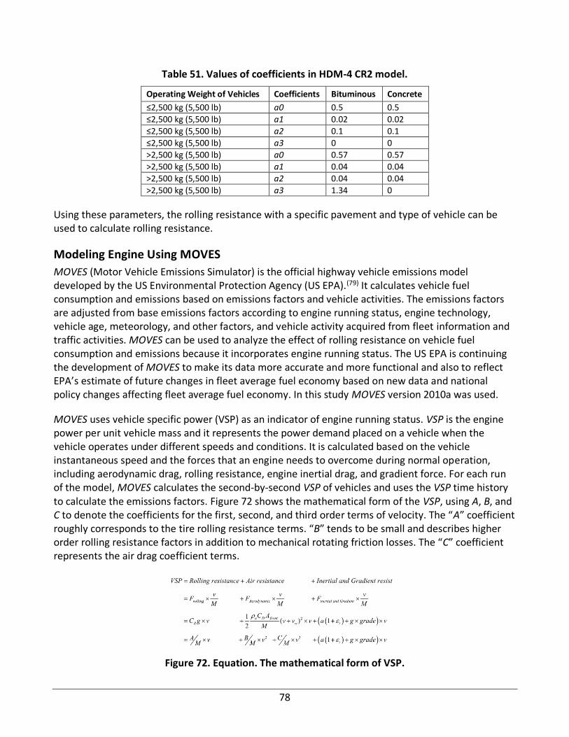
78

Table 51. Values of coefficients in HDM-4 CR2 model.

Operating Weight of Vehicles Coefficients Bituminous Concrete

≤2,500 kg (5,500 lb) a0 0.5 0.5

≤2,500 kg (5,500 lb) a1 0.02 0.02

≤2,500 kg (5,500 lb) a2 0.1 0.1

≤2,500 kg (5,500 lb) a3 0 0

>2,500 kg (5,500 lb) a0 0.57 0.57

>2,500 kg (5,500 lb) a1 0.04 0.04

>2,500 kg (5,500 lb) a2 0.04 0.04

>2,500 kg (5,500 lb) a3 1.34 0

Using these parameters, the rolling resistance with a specific pavement and type of vehicle can be used to calculate rolling resistance.

Modeling Engine Using MOVES

MOVES (Motor Vehicle Emissions Simulator) is the official highway vehicle emissions model developed by the US Environmental Protection Agency (US EPA).(79) It calculates vehicle fuel consumption and emissions based on emissions factors and vehicle activities. The emissions factors are adjusted from base emissions factors according to engine running status, engine technology, vehicle age, meteorology, and other factors, and vehicle activity acquired from fleet information and traffic activities. MOVES can be used to analyze the effect of rolling resistance on vehicle fuel consumption and emissions because it incorporates engine running status. The US EPA is continuing the development of MOVES to make its data more accurate and more functional and also to reflect EPA’s estimate of future changes in fleet average fuel economy based on new data and national policy changes affecting fleet average fuel economy. In this study MOVES version 2010a was used.

MOVES uses vehicle specific power (VSP) as an indicator of engine running status. VSP is the engine power per unit vehicle mass and it represents the power demand placed on a vehicle when the vehicle operates under different speeds and conditions. It is calculated based on the vehicle instantaneous speed and the forces that an engine needs to overcome during normal operation, including aerodynamic drag, rolling resistance, engine inertial drag, and gradient force. For each run of the model, MOVES calculates the second-by-second VSP of vehicles and uses the VSP time history to calculate the emissions factors. Figure 72 shows the mathematical form of the VSP, using A, B, and C to denote the coefficients for the first, second, and third order terms of velocity. The “A” coefficient roughly corresponds to the tire rolling resistance terms. “B” tends to be small and describes higher order rolling resistance factors in addition to mechanical rotating friction losses. The “C” coefficient represents the air drag coefficient terms.

Figure 72. Equation. The mathematical form of VSP.

79

where:

Frolling is the rolling resistance in Newtons;

FAerodynamic is the aerodynamic resistance in Newtons;

Finertial and Gradient is the inertial resistance (if in acceleration) and gradient resistance (if on hill) in Newtons;

CR is the rolling resistance coefficient;

ρa is the ambient air density (1.207 kg/m3, at 20°C);

v is the vehicle speed in m/s;

vw is the speed of headwind into the vehicle in m/s;

Afront is the front area of the vehicle in m2;

CD is the aerodynamic drag coefficient;

εi is the “mass factor,” which is the equivalent translational mass of the rotating components (wheels, gears, shafts, etc.) of the powertrain;

grade is the gradient, which is vertical rise divided by slope length;

g is the acceleration of gravity in m2/s;

M is the mass of vehicles in kg;

a is vehicle acceleration in m2/s;

A is the coefficient of rolling resistance component in MOVES;

B is the coefficient of higher order rolling resistance factors and mechanical rotating friction losses in MOVES; and

C is the coefficient of air drag term in MOVES.

With VSP calculated, the engine running status in MOVES is then defined by both instantaneous VSP and speed. This mode is binned for the development of emissions factor and fuel consumption. MOVES classifies the VSP bin for different modeling purposes: fuel consumption and emissions. Table 52 shows the bin definition for fuel consumption modeling in MOVES.(80)

80

Table 52. MOVES Operating Mode Bin Definitions for Fuel Consumption for Braking (Bin 0)/Idle (Bin 1)

VSP / Instantaneous Speed (mph) 0-25 25-50 >50

< 0 kW/metric ton Bin 11 Bin 21 -

0 to 3 Bin 12 Bin 22 -

3 to 6 Bin 13 Bin 23 -

6 to 9 Bin 14 Bin 24 -

9 to 12 Bin 15 Bin 25 -

12 and greater Bin 16 Bin 26 Bin 36

6 to 12 - - Bin 35

< 6 - - Bin 33

Therefore, the emissions factors are directly related to the VSP, from which the pavement contribution can be included in the vehicle emissions modeling. The user can also input a VSP distribution directly, but under this modeling mode the calculation can only be run at an hourly level, which does not meet the requirements of this study.

Updating the Rolling Resistance Term

According to MOVES documents, the default values of coefficients A, B, and C are derived from the track road load horsepower (TRLHP) at 50 mph recorded in the Mobile Source Observation Database (MSOD).(81) MSOD includes the emissions test data from in-use mobile air pollution sources such as cars, trucks, and engines from trucks and off-road vehicles. Here, TRLHP is a value obtained through dynamometer tests of vehicles, in which a vehicle is running on a smooth surface, usually steel or steel with a sand coating. From this point of view, the rolling resistance coefficient (A) in the MOVES model only includes the rolling resistance effect from vehicles and excludes the effect from pavements but allows the rolling resistance parameter to be proportionally increased to reflect pavement condition.

Figure 73, which is the original equation in HDM-4, implies that the effect of surface characteristics on rolling resistance is a product of the effect from pavement surface and vehicle tires, as indicated by CR2. In MOVES, because the A coefficient is derived from a wide range of dynamometer test results, it can be assumed that this coefficient has included all the averaged effects from the surface on the dynamometer, as well as a variety of vehicle and tires. The A coefficient can be proportionally increased by increasing the effect of surface characteristics from the dynamometer surface to the real-world pavement surface. Because the dynamometer is very smooth and usually uses steel or steel with a sand coating as its surface, which has much lower macrotexture than real pavement, the IRI and MDP are assumed to be 0. Figure 73 shows the relationship between the updated A coefficient and the default A coefficient in the MOVES database. The updated A coefficient is used in later MOVES calculations for emissions and fuel consumption. Although the B coefficient also includes a higher order rolling resistance factor, the B coefficient was not revised for this study because (1) it also combines the rotating friction losses and (2) it is either 0 or very small.

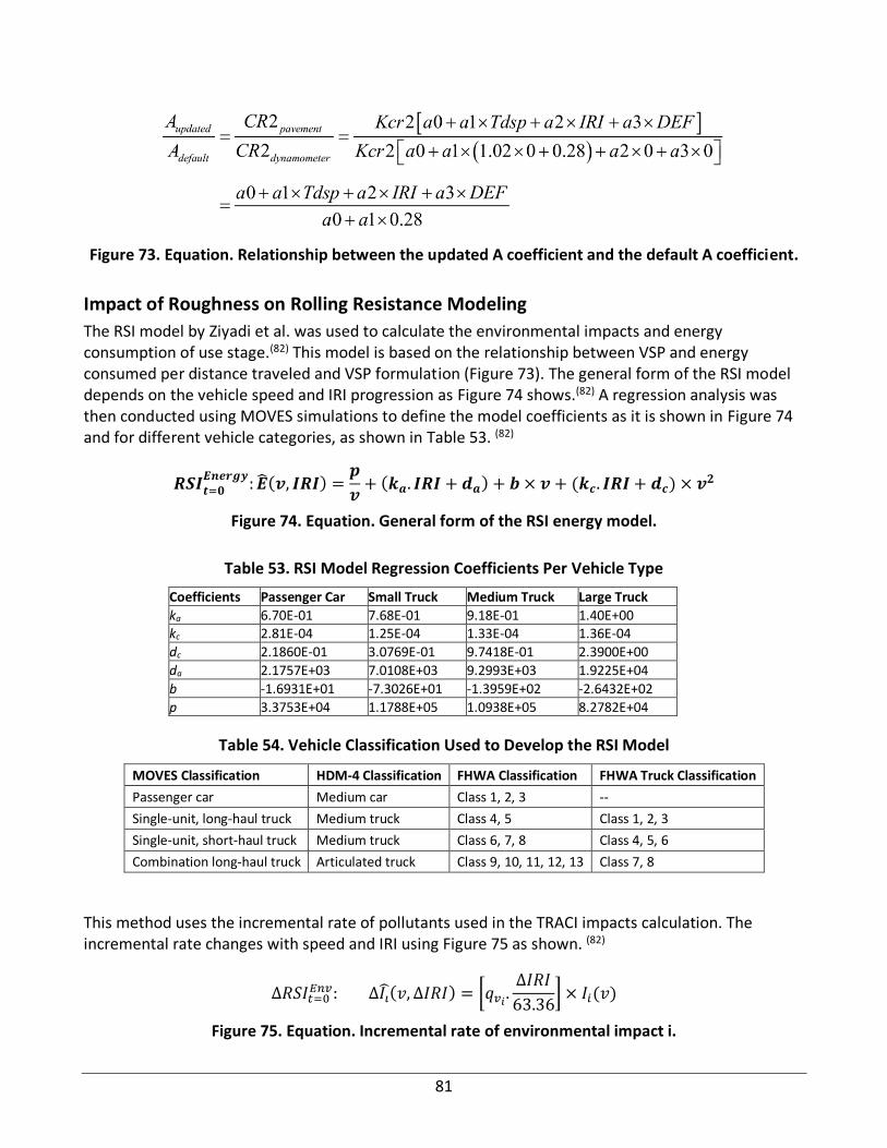
81

Figure 73. Equation. Relationship between the updated A coefficient and the default A coefficient.

Impact of Roughness on Rolling Resistance Modeling

The RSI model by Ziyadi et al. was used to calculate the environmental impacts and energy consumption of use stage.(82) This model is based on the relationship between VSP and energy consumed per distance traveled and VSP formulation (Figure 73). The general form of the RSI model depends on the vehicle speed and IRI progression as Figure 74 shows.(82) A regression analysis was then conducted using MOVES simulations to define the model coefficients as it is shown in Figure 74 and for different vehicle categories, as shown in Table 53. (82)

𝑹𝑺𝑰𝒕=𝟎𝑬𝒏𝒆𝒓𝒈𝒚: �̂�(𝒗, 𝑰𝑹𝑰) =

𝒑

𝒗+ (𝒌𝒂. 𝑰𝑹𝑰 + 𝒅𝒂) + 𝒃 × 𝒗 + (𝒌𝒄. 𝑰𝑹𝑰 + 𝒅𝒄) × 𝒗

𝟐

Figure 74. Equation. General form of the RSI energy model.

Table 53. RSI Model Regression Coefficients Per Vehicle Type

Coefficients Passenger Car Small Truck Medium Truck Large Truck

ka 6.70E-01 7.68E-01 9.18E-01 1.40E+00 kc 2.81E-04 1.25E-04 1.33E-04 1.36E-04

dc 2.1860E-01 3.0769E-01 9.7418E-01 2.3900E+00

da 2.1757E+03 7.0108E+03 9.2993E+03 1.9225E+04

b -1.6931E+01 -7.3026E+01 -1.3959E+02 -2.6432E+02

p 3.3753E+04 1.1788E+05 1.0938E+05 8.2782E+04

Table 54. Vehicle Classification Used to Develop the RSI Model

MOVES Classification HDM-4 Classification FHWA Classification FHWA Truck Classification

Passenger car Medium car Class 1, 2, 3 --

Single-unit, long-haul truck Medium truck Class 4, 5 Class 1, 2, 3

Single-unit, short-haul truck Medium truck Class 6, 7, 8 Class 4, 5, 6

Combination long-haul truck Articulated truck Class 9, 10, 11, 12, 13 Class 7, 8

This method uses the incremental rate of pollutants used in the TRACI impacts calculation. The incremental rate changes with speed and IRI using Figure 75 as shown. (82)

∆𝑅𝑆𝐼𝑡=0𝐸𝑛𝑣: ∆𝐼�̂�(𝑣, ∆𝐼𝑅𝐼) = [𝑞𝑣𝑖 .

∆𝐼𝑅𝐼

63.36] × 𝐼𝑖(𝑣)

Figure 75. Equation. Incremental rate of environmental impact i.

82

Where

𝐼𝑖(𝑣): is the incremental rate of environmental rate i at speed v and qvi is the percent increment of the environmental impact i at a speed v and calculated as Figure 76 shows. (82)

𝑞𝑣𝑖 = 𝑘𝑣𝑖 . 𝑣 + 𝑑𝑣𝑖

Figure 76. Equation. Percent increment of environmental impact i.

𝑘𝑣𝑖 , 𝑑𝑣𝑖 are the increment rate coefficients. Table 55 shows the model coefficients values for

passenger cars per TRACI impact category.(82) The list of environmental impacts do not include ozone depletion and fossil fuel depletion because the results of MOVES simulation showed that these two impacts are not affected by the pollutants used in the RSI model development.

Table 55. Increment Rate Coefficients for Passenger Cars

Impact category i kvi dvi

Global warming 5.88E-04 3.51E-03

Smog 8.06E-04 1.42E-02

Acidification 7.83E-04 1.25E-02

Eutrophication 7.83E-04 1.27E-02

Carcinogenics 7.24E-04 -7.24E-03

Noncarcinogenics 7.59E-05 -9.25E-04

Respiratory effects 1.01E-03 2.80E-03

Ecotoxicity 1.80E-04 -2.05E-03

TEXTURE-RELATED ROLLING RESISTANCE

The texture model developed by Chatti and Zaabar was used to quantify the additional energy consumption due to texture (Figure 77).(83) The model depends on the vehicle speed v.

Figure 77. Equation. Percent change in energy consumption due to texture.

The tool conducts LCA for flexible pavements.(84) The model developed by University of California Pavement Research Center (CPRC) for MPD progression of dense graded AC pavements was incorporated in the tool. This model is shown in Figure 78.(84)

Figure 78. Equation. MPD model for dense graded asphalt concrete pavement.

where NMAS is the nominal maximum aggregate size.

83

Figure 79 is the calibrated version of CPRC model (Figure 78) for use in Illinois. The coefficients shown below can be changed by the user in the tool and be replaced with numbers more representative for the State DOT specifications.

Figure 79. Equation. MPD progression model.

MAINTENANCE AND REHABILITATION SCHEDULE

Maintenance and rehabilitation (M&R) is an essential component in pavement management system (PMS) because it supports strategies to maintain a serviceable condition for pavements and extends pavement service life through various jumps at times of maintenance application. The deterministic performance models and multi-criteria estimation approach (presented in Chapter 5) were used to build M&R schedule that extends over the analysis period calculated based on the alternatives selected by the user. More information about the M&R schedule construction methods are presented in Chapter 8.

The developed tool assumes thin AC overlay to be a default maintenance activity applied every time it is optimum to take an action to maintain the pavement in a good condition. However, in case IRI progression is triggered by cracking threshold then CIR with overlay is applied to enhance structural capacity of the pavement.

WORK ZONE MODELING

Many studies investigated methods to model work zone strategies. Governmental agencies and FHWA developed software tools (e.g., Construction Analysis for Pavement Rehabilitation Strategies [CA4PRS], Kentucky user cost program [KyUCP]) to select strategies for traffic delay management during the construction stage.(85,86) A good traffic management plan prior to construction is important to provide a contractor with an optimal construction window and ensure a better flow of traffic through the work zone. The developed tool assumes that user has already set a traffic management plan and parameters to model the work zone. These parameters are represented in Table 56.

Table 56. Work Zone Parameters Used for Impact Calculation

Work Zone Parameters

Queue length (mile)

Work zone length (mile)

Queue speed (mile)

Work zone speed (mph)

Normal traffic speed (mph)

Passenger car (percent)

Small truck (percent)

Medium truck (percent)

Large truck (percent)

84

Virginia DOT applied CIR and FDR on 3.66 mi of southbound I-81 in August County and monitored the road section performance for three-year service period.(87) The results of the study showed that the in-place recycling techniques were successfully constructed. The traffic management plan of the project consisted of reducing two lanes to one lane for the entire length. A closure window was decided based on traffic data, which reflected times when highest volumes occurred.

85

CHAPTER 7: ANALYSIS AND INTERPRETATION

The developed tool compares energy use and emissions arising during various maintenance and rehabilitation treatments. Additionally, the performance progression over the analysis period is provided. In this chapter, a sensitivity analysis is conducted for various project-level factors.

SENSITIVITY ANALYSIS

Each life-cycle stage is assessed through analyzing the sensitivity of LCIA over the analysis period, considering allocation method, end-of-life scenarios, hauling distance, and pavement hardness. Case studies from field projects are evaluated to validate results of the LCA study conducted using the tool (Appendix F).

Analysis Period

The analysis period is calculated following the approach explained in the pavement LCA framework(1) as the duration from the longest living first major rehabilitation to the end of its subsequent rehabilitation application.

The study is applied on a pavement in a good condition. The sensitivity of the M&R schedule to rehabilitation and maintenance alternatives selection is conducted through two rehabilitation alternatives, which are conventional mill and fill (12 years) and CIR (15 years) and three maintenance scenarios:

• Scenario 1: P1, thin overlay (8 years) (from 3 to 13 years when IRI is used).(88)

• Scenario 2: P2, bituminous surface treatment (BST) (7 years).(89)

• Scenario 3: P1P2, thin overlay + BST.

The goal of this study is to show the impact of the analysis period on the use stage energy for the traffic characteristics presented in Table 57. Table 58 shows the analysis period calculation for the M&R scenarios considered. Because CIR service life is longer compared to mill and fill, AP calculation is based on the time of its subsequent rehabilitation; it is assumed to be the same as the first major rehabilitation.

Table 57. Traffic Assumptions

ADT Truck Percent (%)

Small Truck (%)

Medium Truck (%)

Large Truck (%)

Growth Factor (%)

Average Speed (mph)

2000/8000 10 35 40 25 2 55

Table 58. Analysis Period Sensitivity Analysis Scenarios

M&R Scenario Analysis Period (years)

RP1R 15+8+15 = 38

RP2R 15+7+15 = 37

RP1P2R 15+8+7+15 = 45

86

Figure 80 shows that the M&R schedule, involving more maintenance applications, results in greater annualized energy and higher analysis period at low and high traffic. Furthermore, the use energy is more sensitive to ADT than to analysis period value.

Figure 80. Graph. Annualized energy at use phase and analysis period for different M&R schedules.

End of Life

This section assesses the sensitivity of life-cycle total impacts to allocation method selection, to the recycling rate at end of life, to hauling road type, and to end of life recycling scenario. The analysis was applied on CIR/OL, which is a combination of CIR and 2.5-in-AC overlay treatment for an existing pavement surface of 4 in. The impacts of each life-cycle stage of the CIR/OL project are assessed, and Table 59 presents the processes involved at each stage. The traffic information and AC materials quantities are presented in Table 60 and Table 61, respectively. The analysis schematic is depicted in Figure 81.

Finally, an end-of-life comparative study of two equivalent in-place recycling and conventional method designs was conducted to study the effect of end-of-life factors on different treatment types for the same pavement structure.

It was assumed that AC materials are all virgin and do not contain any RAP content and that the only recyclable materials are AC materials and be used as RAP for the future system.

0

5

10

15

20

25

30

35

40

45

50

0

2000

4000

6000

8000

10000

12000

14000

16000

RP1P2R RP1R RP2R RP1P2R RP1R RP2R

ADT = 2000 ADT = 8000

An

ayls

is p

erio

d (

year

s)

An

nu

aliz

ed u

se e

ner

gy

(GJ/

lan

e-m

ile)

Annualized use energy Analysis period

87

Table 59. Life-Cycle Processes of CIR/OL Treatment

Material Production / Hauling

Construction Use Maintenance

• Asphalt straight binder

• Crushed aggregate

• Natural aggregate

• AC operation

• Cement

• Asphalt emulsion

• Milling machine

• Crusher/pugmill

• Paver

• Pneumatic roller

• Vibratory roller

• Grader

• Water truck

• Service truck

• Dump truck

• Pickup machine

• Work zone

• Roughness

• Texture

• Asphalt straight binder production

• Crushed aggregate production

• Natural aggregate production

• Hauling AC raw material to plant

• Hauling AC, cement, asphalt emulsion to site

• Milling machine

• Paver

• Sweeper

• Vibratory roller

Table 60. Traffic Assumptions

ADT IRI Threshold (inch/mile)

Passenger Car (%)

Small Truck (%)

Medium Truck (%)

Large Truck (%)

Growth Factor (%)

Average Speed (mph)

2000 300 80 4 1 15 4 70

Table 61. Asphalt Concrete Overlay Material Quantities

Material Type Quantities (ton)

Asphalt binder 57.2

Crushed aggregate 705.5

Natural aggregate 213.2

AC 985.1

EOL Allocation Methods

Cut-off and substitution methods were evaluated to assess the impact of allocation method selection in an urban area where all material hauling distances are assumed to be 10 mi and where the pavement is totally recycled on plant at the end of life. Figure 82 and Figure 83 shows that using 100% cut-off results in higher energy and GWP compared to 100% substitution. The total life-cycle energy and GWP show 8.3% and 3.5% reduction, respectively, when using substitution versus cut-off because cut-off allocates all burden of the pavement at end of life to the original pavement; whereas, substitution rewards the original system for producing recyclable materials for the future system.

88

Figure 81. Chart. EOL sensitivity analysis schematic.

Figure 82. Graph. Total life-cycle energy for using 100% substitution versus 100% cut-off (at CPR = central plant recycling).

7.6E+06

7.8E+06

8.0E+06

8.2E+06

8.4E+06

8.6E+06

8.8E+06

100% Cut-off 100% Substitution

Tota

l li

fe c

ycle

en

erg

y (

MJ

/la

ne-m

ile)

Allocation method

89

Figure 83. Graph. Total life-cycle GWP for using 100% substitution versus 100% cut-off (at CPR = central plant recycling).

Recycling Rate

At the end of life, the recycling rate decision affects the total life-cycle impacts. The higher the recycling rate, the more reward is allocated to the original system and the lower the impacts. Figure 84 shows a lower recycling rate at the end of life results in higher environmental impacts when using both cut-off and substitution. However, the cut-off method is less sensitive to the end-of-life recycling rate than substitution because the difference percent of using recycling rates of 80% and 60% versus 100% are 1.0% and 2.1%, respectively. However, substitution impacts at recycling rates of 80% and 60% versus 100% increase by 5.0% and 10.0%, respectively. Therefore, it is recommended to use the substitution method when part of the pavement is recycled. The cut-off method considers the pavement at the end of life as an isolated system responsible for all the burden generated during the life cycle.

Recycling EOL Scenarios

Three scenarios are usually considered at the end of life to manage the use of pavement materials: CPR, IPR, and landfilling. For a case presented herein, a pavement is located in an urban area and is totally recycled at end of life. When using the substitution method, Figure 85 shows that using IPR reduces end-of-life energy by 74.5%; however, it is 10.6% when allocating resources using the cut-off method. Therefore, cut-off is less sensitive to recycling EOL scenarios selection.

1.14E+06

1.15E+06

1.16E+06

1.17E+06

1.18E+06

1.19E+06

1.20E+06

1.21E+06


Tota

l li

fe c

ycle

GW

P (

kg C

O2/l

an

e-m

ile)

Allocation method

90

Figure 84. Graph. Total life-cycle energy and GWP versus different 100% substitution recycling rates.

Figure 85. Graph. Total EOL energy using IPR versus CPR at 100% substitution and cut-off criteria.

7.4E+06

7.6E+06

7.8E+06

8.0E+06

8.2E+06

8.4E+06

8.6E+06

8.8E+06

9.0E+06

60% 80% 100%

Tota

l li

fe c

ycle

en

ergy (

MJ/l

an

e-m

ile)

Recycling rate


0

100000

200000

300000

400000

500000

600000

700000

800000

900000

1000000

CPR IPR

Tota

l E

OL

en

erg

y (

MJ

/la

ne-m

ile)

EOL scenario


91

Road Type

The effect of road type is assessed by calculating the impacts of hauling materials on an urban road (10 mi) versus a rural road (50 mi) when the pavement is recycled at different rates 60%, 80%, and 100% using the CPR scenario. Figure 86 shows that the longer the hauling distance, the larger the impacts. At a hauling distance of 50 mi, the life-cycle energy calculated using substitution is higher than the one calculated with the cut-off method at 60% and 80% recycling rates. In addition, cut-off method is less sensitive to hauling distances from pavement location to central plant and landfill facilities; whereas, substitution is more sensitive to the road type because it accounts for hauling of virgin materials of the original system and hauling of RAP or waste to future systems.

Figure 86. Graph. Sensitivity of energy to cut-off and substitution methods for different road types.

Comparative Study

The following case study was employed to make a comparative energy assessment between the use of CIR/OL and conventional mill and fill (MF). Major factors affecting the comparative energy consumption such as pavement hardness, pavement width, AC hauling distance and hauling road grade were changed to perform a sensitivity analysis. When all major factors are considered for realistic CIR and overlay designs, such sensitivity analysis would allow for evaluation of the range of energy savings.

The existing structure consists of AC (4 in), crushed aggregate base coarse layer (8 in), and crushed granular material (4 in) on top of a subgrade soil having a California Bearing Ratio (CBR) value of 6%. Both designs were conducted based on Chapter 46 of Illinois Department of Transportation Bureau of Local Roads and Streets (IDOT BLRS) manual for pavement rehabilitation.(90) The design procedure for both alternatives assumes typical values of structural coefficients for each material and calculates a remaining structural number (SNR) and a final structural number (SNF) for each layer, which are

7.0E+06

7.5E+06

8.0E+06

8.5E+06

9.0E+06

9.5E+06

1.0E+07

Urban road Rural road Urban road Rural road Urban road Rural road

60% 80% 100%

Tota

l li

fe c

ycle

en

erg

y (

MJ

/lan

e-m

ile)


𝑹𝟐 = 𝟔𝟎% 𝑹𝟐 = 𝟖𝟎% 𝑹𝟐 = 𝟏𝟎𝟎%

92

calculated based on inputs for traffic levels, subgrade strength, and existing layer thicknesses. The required thickness of the overlay is then calculated based on the difference between the two structural numbers.

The design was used for a low-volume road with a traffic factor of 0.65, equivalent to an average daily traffic of 2,041 vehicles/day with 7.5% single-unit trucks and 2.5% multiple unit trucks. For the CIR with an overlay design alternative, the existing 4 in AC was recycled. The SNR and SNF were calculated to be 2.24 and 3.25, respectively, which requires an additional overlay thickness of 2.5 in on top of the recycled AC. For the mill and fill design alternative, in contrast, the top 2 in of AC was milled, thus resulting in calculated values of 1.84 and 3.25 for SNR and SNF, respectively, and an additional overlay thickness of 4 in.

Figure 87 shows that MF produces higher life-cycle energy compared with CIR/OL: approximately 19.2 million MJ/lane-mile using a 100% cut-off and 18.01 million MJ/lane-mile using 100% substitution. CIR/OL method results in 54.3% and 55.4% less energy than MF when cut-off and substitution were used, respectively. Hence, allocation methods are independent of in-place and conventional designs.

Figure 87. Graph. Comparison of CIR and MF life-cycle energy at 100% cut-off and 100% substitution methods.

0.0E+00

5.0E+06

1.0E+07

1.5E+07

2.0E+07

2.5E+07

CIR/OL MF

Tota

l li

fe c

ycle

en

erg

y (

MJ

/la

ne-m

ile)

Treatment type


93

MAJOR ASSUMPTIONS AND LIMITATIONS

The following are limitations of the tool:

• More M&R realistic schedule is needed to better trigger performance over the analysis period.

• LCCA is not considered in the study.

• Deterministic models are limited to one region.

• The tool generates results that have embedded uncertainties. Therefore, a quantitative uncertainty should be considered.

• Use stage is limited to roughness and texture; hence, albedo and pavement deflection should be considered.

• The equipment inventory should be updated regularly.

94

CHAPTER 8: TOOL DEVELOPMENT

PROGRAMMING PLATFORM

The IPR tool is developed using visual basic applications (VBA) in Microsoft® Excel. VBA is an event-driven programming language from Microsoft. The VBA allows the use of the tool by all transportation project stakeholders and access inventory databases and performance models. The developed tool is a series of linked user forms operated by macros (programmed instructions to automate a task) that allow modeling the environmental impacts and performance of projects selected through databases built in the tool Excel file worksheets. The user form is a user-friendly interactive platform to enter data required to compile the final outputs. The tool key terms as they are used in this report are defined in Table 62.

Table 62. Tool Key Terms Definition

Key Term Definition

Worksheet A MS Excel worksheet or sheet is a single page in a MS Excel workbook (Figure 88).

Table A MS table is a special object available in MS Excel that contains column headers and advanced properties.

Form controls A MS Excel form control is an interactive button, checkbox, or other visual control that is directly implemented on a worksheet.

Command button A user-form control used to run a macro.

Checkbox A user-form control used to indicate a Boolean choice.

Combobox A user-form control to create a dropdown list.

Page A control existing on user-forms that contain sections associated to different project aspects.

Default button Form control that is clicked to generate data extracted from primary data collected.

The features that highlight the user-friendly quality of the developed tool are listed below:

• Worksheets are used as a platform to report data and review results.

• The worksheet interfaces include form controls to guide the user in the project analysis.

• Invalid user inputs or questionable user choices are checked by displaying an error message.

• Projects results reports can be downloaded in pdf format.

95

Figure 88. Photo. Project inputs worksheet.

MODULES

The tool includes five modules: materials, construction, work zone, use, and end of life. The user can select up to five maintenance or rehabilitation treatments candidates from the list reported in Table 63 as alternatives for analyses.

Table 63. List of Maintenance and Rehabilitation Treatments Considered for Project Selection

Maintenance Treatments Rehabilitation Treatments

Cape seal CIR

Chip seal double course CIR + cape seal

Chip seal single course CIR + chip seal

Fog seal CIR + medium overlay (between 2 and 4 in)

HIR remixing CIR + thick overlay (over 4 in)

HIR remixing + medium overlay (between 2 and 4 in) CIR + thin overlay (2 in or less)

HIR remixing + thick overlay (over 4 in) Cold milling + medium overlay (between 2 and 4 in)

HIR remixing + thin overlay (2 in or less) Cold milling + thick overlay (over 4 in)

HIR repaving Cold milling + thin overlay (2 in or less)

HIR resurfacing FDR

HIR resurfacing + medium overlay (between 2 and 4 in) FDR + medium overlay (between 2 and 4 in)

HIR resurfacing + thick overlay (over 4 in) FDR + thick overlay (over 4 in)

HIR resurfacing + thin overlay (2 in or less) FDR + thin overlay (2 in or less)

Microsurfacing double course FDR + Chip Seal

Microsurfacing single course FDR + Chip Seal

Sand seal

Slurry seal

Thin AC overlay (2 in or less)

Ultra-thin bonded wearing course

96

The user inputs required data in the five modules for environmental impacts and energy use calculation, which are summarized in a worksheet and a breakdown chart, as shown in Figure 89.

Figure 89. Chart. Projects selection process schematic (M/R = maintenance or rehabilitation).

General Inputs

The “Main Inputs” user form has key items to perform life-cycle analysis, as illustrated in Figure 90. These inputs are entered in the user form presented in Figure 91 before the treatment selection. All general inputs entered by the user are automatically reported in “Main Inputs” spreadsheet shown in Figure 92.

Figure 90. Chart. Impact assessment and project main inputs dependencies.

97

Figure 91. Photo. “Main Inputs” user form pages.

Figure 92. Photo. “Main Inputs” spreadsheet.

Treatment Selection

The treatment selection occurs after entering the project’s main inputs. Figure 93 shows an example of “CIR + Medium Overlay (between 2 to 4 in)” selection from the list of treatments displayed in the “Treatment Selection” user form. The number of treatments selected can be up to five and listed in the “Treatments for Analysis” user form with their corresponding performance score and risk level on performance, as illustrated in Figure 94.

98

Figure 93. Photo. Example of a selected treatment in the “Treatment Selection” user form.

99

Figure 94. Photo. “Treatment for Analysis” user form.

Pavement Performance

The pavement performance analysis is important to present the expected life of the treatment and expected change in condition after applying a rehabilitation or a maintenance treatment over the analysis period. There are various descriptors that can be used to assess pavement performance such as IRI, wheel-path cracking percent, pavement condition index, etc. In the tool, the performance models used in California were selected. Because the tool is designed to be applied on a national scale, two options were provided to the user to estimate life expectancy of the treatment selected (Figure 95). First, the life expectancy range [Lmin, Lmax] of all treatments considered in the scope the project is estimated using data from literature. Performance score (PS) is evaluated using multi-criteria performance estimation approach and then used to estimate the treatment life expectancy as follows:

1. PS is 4 or 5: Ideal on-site conditions for selected treatment, indicating very low risk for performance. Treatment life can be expected to be at the highest range, Lmax.

2. PS is 2 or 3: Conditions are fair carrying medium risk for the performance of selected treatment. Treatment life can be expected to be at medium range of expectations, (Lmax + Lmin)/2.

100

3. PS is 1: On-site conditions are not appropriate for the selected treatment with very high risk. Treatment life may be predicted at lower range of expected values, Lmin.

The estimated service life using the first approach produces a default M&R schedule that the user visualizes on the “Life Expectancy” user form, as shown in Figure 96.

The second option is using deterministic performance models to predict the performance progression. The service life is triggered by default IRI threshold; if cracking model is selected, then the performance is further triggered by cracking threshold. The cracking model is a good option to trigger the performance when the pavement has severe structural problems.

Figure 95. Chart. Life expectancy estimation approaches flowchart.

101

Figure 96. Photo. “Life Expectancy” user form.

The pavement management plan of a project requires building a M&R schedule to model the timings when maintenance or rehabilitation actions are applied on the pavement during the analysis period. According to Figure 97, the tool provides two options to build an M&R schedule. The first option uses a simple linear IRI progression that depends on IRI threshold and life estimated for the treatment selected and the future maintenance actions. The user can change the IRI threshold and the treatment life using a slider in “UF_Use” user form. The second method builds the M&R schedule using, at most, four criteria: maximum treatment life, IRI threshold, cracking threshold, and routine maintenance interval. The final M&R schedule can be visualized on the “Information_Treatment” worksheet.

102

Figure 97. Chart. M&R schedule construction options flowchart.

Future maintenance activities are decided by the tool based on the predicted cracking performance of the pavement. Therefore, whenever the cracking performance is triggered by the wheel-path cracking threshold, CIR + thin overlay is applied as an emergency maintenance; otherwise, thin overlay is applied as a preventive maintenance, as illustrated in Figure 98.

Figure 98. Chart. Future maintenance and rehabilitation strategy schematic.

103

Materials Extraction and Production Stage

The user is shown the “Materials” page of “Life-Cycle Inventory” user form (Figure 99) upon clicking “Open LCIA Module” command button. In this page, the user either selects materials and enters the corresponding quantities or uses default materials list and quantities upon clicking “Default” command button.

Figure 99. Photo. “Life-Cycle Inventory” user form, “Materials” page.

In addition, the user can specify pavement design materials by clicking “Custom Design,” as illustrated in Figure 99, and then the user is shown the “Pavement Design” page (Figure 100). For example, if the user selects a combination of a major rehabilitation and microsurfacing or slurry seal, then “Microsurfacing and Slurry Seal” frame is enabled and it is required to input the thickness of aggregate or sand application as well as the application rate (by weight percent of aggregate) of asphalt products (e.g., asphalt binder, emulsion). Whereas, if fog seal, sand seal, or chip seal is selected, then “Fog Seal, Sand Seal and Chip Seal” frame is enabled and it is required to input the application rate of each material for the surface treatment by lb/yd2 unit. Finally, if cape seal is selected, then both “Microsurfacing and Slurry Seal” and “Fog Seal, Sand Seal and Chip Seal” framed are enabled because cape seal is a combination of slurry seal or microsurfacing and chip seal.

In addition, the user is asked to input material information necessary for the construction of the treated pavement layers. If any of the in-place recycling treatment is selected, then the user needs to

104

input the pavement recycled thickness. Furthermore, if AC operation is selected in one of the materials list, then “Edit AC design” command button to enter mix design characteristics and mix materials types and proportions, as Figure 101 shows.

Figure 100. Photo. “Life-Cycle Inventory” user form, “Pavement Design” page.

105

Figure 101. Photo. “Life-Cycle Inventory” user form, “Mix Design” page.

The final stage in the “Materials” page should be filling hauling distances for the selected materials, as shown in Figure 99. The hauling distance can be either to plant or to site. If the user selects the customization option, then AC raw materials hauling distances to plant are entered in the “Mix Design” page (Figure 101), while the AC hauling to site is entered in the “Materials” page (Figure 99).

Construction Stage

At the construction stage, the user should select the equipment used to operate the construction activities in the “Equipment” page of “Life-Cycle Inventory” user form, which is visible upon clicking “Open LCIA Module” command button, shown in Figure 102. The inputs required to enter are fuel type, equipment type, HP bin, tier category, fuel efficiency, speed, and number of passes. These inputs can also be generated upon clicking the “Default” command button. The default equipment units represent the equipment data collected from contractors.

106

Figure 102. Photo. “Life-Cycle Inventory” user form, “Equipment” page.

The construction stage accounts for the work zone as well. The user enters work zone inputs in the “Work Zone” user form, shown in Figure 103, upon clicking the “Open Work Zone Module” command button.

107

Figure 103. Photo. “Work Zone” user form.

Maintenance and Rehabilitation Stage

The ultimate outcome from the “Life Expectancy” user form is to obtain an M&R schedule. The M&R schedule is necessary to compile the impacts of the use and maintenance stages. Figure 104 shows example of a default M&R schedule for a threshold of 300 in/mi and service life estimated to be 20 years, and a deterministic M&R schedule that shows when IRI progression is triggered by cracking threshold (Figure 105). As Figure 97 shows, the deterministic M&R schedule is obtained using up to five criteria and displayed in the “Create Schedule” user form, shown in Figure 106.

108

Figure 104. Photo. Default M&R schedule.

Figure 105. Photo. M&R built using deterministic models.

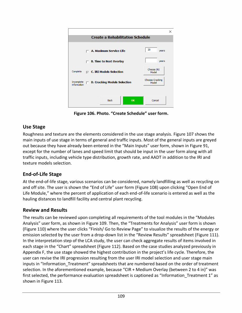
109

Figure 106. Photo. “Create Schedule” user form.

Use Stage

Roughness and texture are the elements considered in the use stage analysis. Figure 107 shows the main inputs of use stage in terms of general and traffic inputs. Most of the general inputs are greyed out because they have already been entered in the “Main Inputs” user form, shown in Figure 91, except for the number of lanes and speed limit that should be input in the user form along with all traffic inputs, including vehicle type distribution, growth rate, and AADT in addition to the IRI and texture models selection.

End-of-Life Stage

At the end-of-life stage, various scenarios can be considered, namely landfilling as well as recycling on and off site. The user is shown the “End of Life” user form (Figure 108) upon clicking “Open End of Life Module,” where the percent of application of each end-of-life scenario is entered as well as the hauling distances to landfill facility and central plant recycling.

Review and Results

The results can be reviewed upon completing all requirements of the tool modules in the “Modules Analysis” user form, as shown in Figure 109. Then, the “Treatments for Analysis” user form is shown (Figure 110) where the user clicks “Finish/ Go to Review Page” to visualize the results of the energy or emission selected by the user from a drop-down list in the “Review Results” spreadsheet (Figure 111). In the interpretation step of the LCA study, the user can check aggregate results of items involved in each stage in the “Chart” spreadsheet (Figure 112). Based on the case studies analyzed previously in Appendix F, the use stage showed the highest contribution in the project’s life cycle. Therefore, the user can revise the IRI progression resulting from the user IRI model selection and user stage main inputs in “Information_Treatment” spreadsheets that are numbered based on the order of treatment selection. In the aforementioned example, because “CIR + Medium Overlay (between 2 to 4 in)” was first selected, the performance evaluation spreadsheet is captioned as “Information_Treatment 1” as shown in Figure 113.

110

Figure 107. Photo. “Use Stage” user form, “Texture” page.

Figure 108. Photo. “End of Life” user form.

111

Figure 109. Photo. Requirements completed before reviewing the final results.

Figure 110. Photo. Completed analysis prior to clicking Finish/Go to Review Page button.

112

Figure 111. Photo. Review of total results of each life-cycle stage.

Figure 112. Photo. Breakdown chart of the final results for CIR + Medium Overlay (between 2 to 4 in).

113

Figure 113. Photo. Use phase main inputs and IRI progression of “CIR + Medium Overlay (between 2 to 4 in)” treatment.

CALCULATIONS

Materials: Extraction and Production

The inputs used to calculate materials production and extraction impacts are shown in Table 64. The impacts are computed following the formula in Figure 114.

Table 64. Key Items of Materials Selection (“LCIA” User Form / “Materials” Page)

Key items Description

Material type The user selects a treatment type from a dropdown.

Quantity (ton) Quantity of material selected.

Figure 114. Equation. Material impact calculation formula.

Materials quantities can be either input by the user or calculated by the tool at the customization level using material characterization listed in Table 65 and Figure 100.

114

Table 65. Assumptions of Default Treatment Materials

Treatment Type Material Characterization

Cape Seal Chip seal: 0.3gal/yd2 of emulsion, 23 lb/yd2 of aggregate Slurry seal: 16lb/yd2 of aggregate, 16 percent emulsion of aggregate wt

Chip Seal Double Course 0.8 gal/yd2, 60 lb/yd2

Chip Seal Single Course 0.425 gal/yd2, 30 lb/yd2 of aggregate

CIR 4% emulsion, 1% cement

FDR 4% emulsion, 2% cement, 2 in crushed aggregate

Fog Seal 0.13 gal/yd2 (emulsion)

HIR Remixing 0.18 L/m2 (rejuvenator)

HIR Repaving 0.18 L/m2 (rejuvenator) + 2 in AC (4% air voids, 6% asphalt content, Gmm: 2.5)

HIR Resurfacing 0.18 L/m2 (rejuvenator)

Microsurfacing Double Course 66 lb/yd2 (agg), 16% wt of emulsified asphalt, 3% wt of mineral filler

Microsurfacing Single Course 33lb/yd2(agg),8% wt of emulsified asphalt, 1.5% wt of mineral filler

Cold Milling + Thin Overlay (2 inches or less) 4% air voids, 6% asphalt content, Gmm: 2.5

Cold Milling + Medium Overlay (between 2 and 4 inches)

4 in (4 air voids, 6% asphalt content, Gmm: 2.5)

Cold Milling + Thick Overlay (over 4 inches) 6 in (4% air voids, 6% asphalt content, Gmm: 2.5)

Sand Seal asphalt materials: 0.25 gal/yd2, agg: 18 lb/yd2

Slurry Seal agg: 20l g/yd2, emulsion: 10.5% wt of agg, mineral filler: 1.8% wt of agg

Thin HMA Overlay (2 inches or less) 2 in (4% air voids, 6% asphalt content, Gmm: 2.5)

Ultra-Thin Bonded Wearing Course 93 lb/yd2 (AC, 5% binder), 0.2gal/yd2 (emulsion)

If the user selects a surface treatment, then the corresponding surface treatment frame in the “Pavement Design” page is enabled. For microsurfacing and slurry seal, the quantity (ton.sh) of aggregate or sand is calculated as in Figure 115, assuming that aggregate/sand density 𝝆𝒂𝒈𝒈/𝒔𝒂𝒏𝒅 is

140 pcf:

𝑄𝑎𝑔𝑔/𝑠𝑎𝑛𝑑 = 𝜌𝑎𝑔𝑔/𝑠𝑎𝑛𝑑(𝑝𝑐𝑓) × 𝑙𝑒𝑛𝑔𝑡ℎ(𝑚𝑖𝑙𝑒) × 𝑤𝑖𝑑𝑡ℎ(𝑓𝑡) × 𝑡ℎ𝑖𝑐𝑘𝑛𝑒𝑠𝑠(𝑖𝑛𝑐ℎ)

× 𝑐𝑜𝑛𝑣𝑒𝑟𝑠𝑖𝑜𝑛 𝑓𝑎𝑐𝑡𝑜𝑟

Figure 115. Equation. Microsurfacing and slurry seal aggregate and sand quantity calculation formula.

The quantity (ton.sh) of an asphalt agent or other material used in a surface treatment is related to its application rate and to the quantity of aggregate or sand as Figure 115 and Figure 116 show.

𝑄𝑎𝑠𝑝ℎ𝑎𝑙𝑡 𝑎𝑔𝑒𝑛𝑡 = 𝑄𝑎𝑔𝑔/𝑠𝑎𝑛𝑑 × 𝑎𝑠𝑝ℎ𝑎𝑙𝑡 𝑎𝑔𝑒𝑛𝑡 𝑎𝑝𝑝𝑙𝑖𝑐𝑎𝑡𝑖𝑜𝑛 𝑝𝑒𝑟𝑐𝑒𝑛𝑡 (%)/100

Figure 116. Equation. Microsurfacing and slurry seal asphalt agent quantity calculation formula.

For fog seal, sand seal, and chip seal, as soon as the application rates (lb/yd2) of each material are entered, the quantities (ton.sh) are calculated as shown in Figure 117.

115

𝑄𝑚𝑎𝑡𝑒𝑟𝑖𝑎𝑙 = 𝑀𝑎𝑡𝑒𝑟𝑖𝑎𝑙 𝑎𝑝𝑝𝑙𝑖𝑐𝑎𝑡𝑖𝑜𝑛 𝑟𝑎𝑡𝑒 (𝑙𝑏

𝑆𝑌) × 𝑙𝑒𝑛𝑔𝑡ℎ(𝑚𝑖𝑙𝑒) × 𝑤𝑖𝑑𝑡ℎ(𝑓𝑡) × 𝑐𝑜𝑛𝑣𝑒𝑟𝑠𝑖𝑜𝑛 𝑓𝑎𝑐𝑡𝑜𝑟

/2000

Figure 116. Equation. Fog seal, sand seal, and chip seal material quantity calculation formula.

The user selects materials for each pavement layer. For wearing and binder courses, the “Material 1” combo box is limited to the list presented in Table 66.

Table 66. “Material 1” Combo Box List

“Material 1” List

Natural aggregate

Crushed aggregate

Sand

AC

The quantity calculation of the materials selected in “Material 2” and “Material 3” combo boxes depends on “Material 1” type’s quantity, as shown in Figure 118.

Figure 117. Equation. Material 2 and 3 quantity calculation formula.

If one of the pavement layers is recycled, then “Material 2” and “Material 3” quantities are calculated, as shown in Figure 119.

𝑄𝑚𝑎𝑡𝑒𝑟𝑖𝑎𝑙 2∕ 3 = (𝛿𝑎𝑔𝑔 𝑠𝑎𝑛𝑑⁄ × 𝑇ℎ𝑖𝑐𝑘𝑛𝑒𝑠𝑠𝑎𝑔𝑔 𝑠𝑎𝑛𝑑⁄ + 𝑇ℎ𝑖𝑐𝑘𝑛𝑒𝑠𝑠𝑟𝑒𝑐𝑦𝑐𝑙𝑒𝑑)(𝑖𝑛𝑐ℎ) × 𝑙𝑒𝑛𝑔𝑡ℎ(𝑚𝑖𝑙𝑒)

× 𝑤𝑖𝑑𝑡ℎ(𝑓𝑡) × 2 × 𝑀𝑎𝑡𝑒𝑟𝑖𝑎𝑙2∕3 𝑎𝑝𝑝𝑙𝑖𝑐𝑎𝑡𝑖𝑜𝑛 𝑝𝑒𝑟𝑐𝑒𝑛𝑡 (%) × 𝑐𝑜𝑛𝑣𝑒𝑟𝑠𝑖𝑜𝑛 𝑓𝑎𝑐𝑡𝑜𝑟

/100

Figure 118. Equation. Material 2 and 3 quantity calculation formula for a recycled layer.

where:

equal to 1 when aggregate or sand is used and equal to 0 otherwise.

thickness of the layer where aggregate and/or sand is used in inch.

thickness of the recycled layer in inch.

When AC is selected, a number of key items listed in Table 67 should be entered in the “Mix Design” page to calculate AC quantity.

𝑄𝑀𝑎𝑡𝑒𝑟𝑖𝑎𝑙 2/3 = 𝑄𝑀𝑎𝑡𝑒𝑟𝑖𝑎𝑙 1 ×𝑀𝑎𝑡𝑒𝑟𝑖𝑎𝑙2/3 𝑝𝑒𝑟𝑐𝑒𝑛𝑡 𝑜𝑓 𝑎𝑝𝑝𝑙𝑖𝑐𝑎𝑡𝑖𝑜𝑛/100

116

Table 67. Key Items of Mix Design Calculation (“LCIA” User Form / “Mix Design” Page)

Key Items Description

Gmm Maximum specific gravity of the compacted paving AC mixture, “edit mix” button in the “Pavement Design” page.

Air voids (percent) Air voids percentage.

Asphalt content (percent)

Asphalt content by weight of mix.

Material type The user selects a material type from a dropdown list.

Recycled binder (percent)

Percent of recycled binder existing in recycled aggregates.

Amount (percent); aggregate to total aggregate wt

Proportion of aggregate i by weight of total aggregates selected.

Thus, the quantities of AC, different types of aggregate selected, and virgin binder are calculated as shown in Figure 120, Figure 121, and Figure 122, respectively.

𝑄𝐴𝐶 = 𝐺𝑠𝑏 × 0.8428 × 𝑙𝑒𝑛𝑔𝑡ℎ(𝑚𝑖𝑙𝑒) × 𝑤𝑖𝑑𝑡ℎ(𝑓𝑡) × 𝑡ℎ𝑖𝑐𝑘𝑛𝑒𝑠𝑠(𝑖𝑛𝑐ℎ) × 𝑐𝑜𝑛𝑣𝑒𝑟𝑠𝑖𝑜𝑛𝑓𝑎𝑐𝑡𝑜𝑟

Figure 119. Equation. AC quantity calculation formula.

where:

𝐺𝑠𝑏 bulk specific gravity.

Length Pavement length in mile.

Width Pavement width in ft.

thickness thickness of AC overlay in inch.

Qagg,i = 𝑄𝐴𝐶 × 𝐴𝑔𝑔𝐴𝐶,𝑖/100

Figure 120. Equation. Aggregate type I quantity calculation formula.

Quantity of aggregate type 𝑖 in ton.sh/lane.mile.inch

Quantity of AC in ton.sh/lane.mile.inch

Percent of aggregate type 𝑖 in AC

Qvirgin binder = 𝑄𝐴𝐶 ×𝐵𝑖𝑛𝑑𝑒𝑟𝐴𝐶

𝑉𝑖𝑟𝑔𝑖𝑛

100

Figure 121. Equation. Virgin binder quantity calculation.

𝑄𝑣𝑖𝑟𝑔𝑖𝑛 𝑏𝑖𝑛𝑑𝑒𝑟 Quantity of virgin binder in ton.sh/lane.mile.inch.

𝐵𝑖𝑛𝑑𝑒𝑟𝐻𝑀𝐴𝑉𝑖𝑟𝑔𝑖𝑛

Percent of virgin binder in AC

117

Once all mix design parameters are entered, the amount of each mix design material is calculated upon clicking the “Calculate” command button. More details about the calculation of AC materials quantities are found in Appendix E.

Hauling

The materials hauling impact assessment is performed using a model that calculates environmental emissions and energy use during the hauling stage at various geometric and environmental hauling trip conditions using the formula in Figure 123 and user inputs listed in Table 68.

𝐸𝐻𝑎𝑢𝑙 = 𝑈𝑛𝑖𝑡 𝑝𝑟𝑜𝑐𝑒𝑠𝑠 𝐸(𝑔𝑟𝑎𝑑𝑒, 𝑡𝑒𝑚𝑝𝑒𝑟𝑎𝑡𝑢𝑟𝑒, 𝑅𝐻, ℎ𝑎𝑢𝑙𝑖𝑛𝑔 𝑚𝑜𝑑𝑒)(𝑡𝑜𝑛.𝑚𝑖𝑙𝑒) × 𝑞𝑢𝑎𝑛𝑡𝑖𝑡𝑦(𝑡𝑜𝑛)× ℎ𝑎𝑢𝑙𝑖𝑛𝑔 𝑑𝑖𝑠𝑡𝑎𝑛𝑐𝑒(𝑚𝑖𝑙𝑒)

Figure 122. Equation. General form for hauling impacts calculation.

Table 68. User Inputs for Hauling Impacts Calculation

Key Items Description User Form Name

Grade The user selects the grade from this range [−8%, 8%]. “Main Inputs”

Temperature The user selects the average temperature of the hauling trip in this range [0ºF, 110ºF].

“Main Inputs”

RH The user selects the relative humidity rate of the hauling trip in this range [0%, 100%].

“Main Inputs”

Supplier-to-site distance (mile) Distance traveled to ship the material (processed) selected to site in miles.

“LCIA”/ “Materials” Page

Supplier-to-plant distance (mile) Distance traveled to ship the material (raw) selected to plant in miles.

“LCIA”/ “Materials” Page

Therefore, the hauling impacts of materials are composed of the hauling from supplier to plant and hauling from supplier to site.

For the raw materials used in AC, the hauling distance is from supplier to plant, which is input in Figure 124. Thus, the hauling impacts are calculated as follows:

Figure 123. Equation. HMA hauling impacts calculation.

where:

𝐸𝐻𝑎𝑢𝑙𝐴𝐶 Impact of hauling AC to site and AC raw materials to plant.

AC overlay thickness in inch.

AC quantity in tons per lane.mile.inch

𝐸𝐻𝑎𝑢𝑙𝐴𝐶 = 𝑡ℎ𝑖𝑐𝑘𝑛𝑒𝑠𝑠 × ( (𝑄𝐴𝐶 × 𝑃𝑖 ,𝐴𝐶 × 𝐻𝑖 × 𝑈𝑛𝑖𝑡 𝑝𝑟𝑜𝑐𝑒𝑠𝑠 𝐸𝐻𝑎𝑢𝑙 )+ 𝑄𝐴𝐶 × 𝐵𝑖𝑛𝑑𝑒𝑟𝐴𝐶

𝑣𝑖𝑟𝑔𝑖𝑛

𝑖

×𝐻𝑏𝑖𝑛𝑑𝑒𝑟 × 𝑈𝑛𝑖𝑡 𝑝𝑟𝑜𝑐𝑒𝑠𝑠 𝐸𝐻𝑎𝑢𝑙

118

Percent of aggregate type 𝑖 in AC.

Hauling distance of aggregate type 𝑖 to plant in mile.

Hauling unit process per mile traveled and ton.sh

𝐵𝑖𝑛𝑑𝑒𝑟𝐴𝐶𝑣𝑖𝑟𝑔𝑖𝑛

Percent of virgin binder in AC.

Hauling distance of binder to plant.

Construction

On-site Equipment

At the construction module, the user is asked to input information about the equipment used on-site to perform the construction activities. Up to 27 equipment types can be selected. The on-site equipment impacts are calculated using the formula in Figure 125 and the user inputs are listed in Table 69.

𝐸𝐸𝑞𝑢𝑖𝑝 = 𝑈𝑛𝑖𝑡 𝑝𝑟𝑜𝑐𝑒𝑠𝑠 𝐸𝐸𝑞𝑢𝑖𝑝(𝑓𝑢𝑒𝑙 𝑡𝑦𝑝𝑒, 𝑡𝑖𝑒𝑟, 𝑒𝑞𝑢𝑖𝑝𝑚𝑒𝑛𝑡 𝑡𝑦𝑝𝑒)(1 𝑔𝑎𝑙⁄ )

×𝑓𝑢𝑒𝑙 𝑐𝑜𝑛𝑠𝑢𝑚𝑝𝑡𝑖𝑜𝑛 (

𝑔𝑎𝑙ℎ𝑜𝑢𝑟)

𝑠𝑝𝑒𝑒𝑑 (𝑓𝑡𝑚𝑖𝑛𝑢𝑡𝑒)

× 𝑛𝑢𝑚𝑏𝑒𝑟 𝑜𝑓 𝑝𝑎𝑠𝑠𝑒𝑠

Figure 124. Equation. On-site equipment impact calculation formula

Table 69. List of User Inputs for the Construction Module (“LCIA”/ “Equipment” Page)

Key Item Description

Fuel type The user chooses diesel, propane in the fuel type dropdown menu.

Equipment type The user selects an equipment type that filters the possible hp in the next input.

HP bin Possible HP ranges for the equipment selected. Once selected, it filters applicable tier categories.

Tier category Set of emissions regulations established by EPA (base, T0, T1, T2, T3, T3B, T4, T4A, T4N).

Fuel consumption In gal/hour, the hourly equipment productivity.

Speed Off-highway and trucks speed on-site in ft/minute.

Number of passes The number of passes that the equipment performs during the construction phase.

Work Zone

The difference in impacts between a normal and a delayed traffic flow represents the work zone impacts contribution, as shown in Figure 126. Figure 127 shows an example of a traffic delay model for a pavement rehabilitation or maintenance project. The RSI model explained in Chapter 6 was used to determine work zone impacts. This model has two main variables: IRI and speed. The unit processes are categorized by vehicle type (i.e., passenger car, small truck, medium truck, large truck). The average of IRI progression defined in-use stage analysis as well as speeds of the normal and delayed traffic due to work zone are used to apply RSI model.

119

Figure 125. Equation. Work zone impact calculation formula.

where:

Additional impact due to work zone

Impact resulting from traffic in the queue zone

Impact resulting from traffic in the work zone

Impact resulting from traffic after exiting work zone

Impact resulting from a normal traffic

Figure 126. Photo. Example of work zone illustration.

Maintenance and Rehabilitation

The maintenance stage accounts for the materials produced, hauled to site and operations to execute the maintenance construction activities. The maintenance stage calculation depends on the number of maintenance activities applied over the analysis period, as shown in Figure 128.

𝐸𝑀𝑎𝑖𝑛𝑡 = (𝐸𝑀𝑎𝑡 + 𝐸𝐸𝑞𝑢𝑖𝑝) × 𝑛𝑢𝑚𝑏𝑒𝑟𝑜𝑓 𝑚𝑎𝑖𝑛𝑡𝑒𝑛𝑎𝑛𝑐𝑒 𝑎𝑝𝑝𝑙𝑖𝑐𝑎𝑡𝑖𝑜𝑛𝑠

Figure 127. Equation. Maintenance stage impact calculation.

120

where:

𝐸𝑀𝑎𝑖𝑛𝑡 Impact resulting from maintenance stage

𝐸𝑀𝑎𝑡

Impact resulting from production and hauling of materials used in the maintenance activity

𝐸𝐸𝑞𝑢𝑖𝑝 Impact resulting from equipment used to operate maintenance construction activities

Use

The use stage impacts calculation is described in Chapter 6. Key items of the use stage impact quantification are listed in Table 70.

Table 70. Use Stage Inputs

Key Item Description Treatment life Life estimated of the treatment life selected

IRI model IRI model selected to describe roughness progression

AADT Average annual daily traffic

Number of lanes Number of lanes of the road to rehabilitate

Average speed Average speed tracked on the road under study

Truck percent Truck percent tracked on the road under study

End of Life

The cumulative environmental impacts of end of life are determined using the cut-off allocation method. The impacts of the end of life stage are produced by the demolition process, disposal of waste material and hauling it to a landfill facility, and/or hauling of landfilled material to central plant recycling. The key items of the end of life impact assessment are listed in Table 71. More details about the end of life impact calculation are found in Chapter 4.

Table 71. End of Life Key Items

Key Item Description

Landfill application rate (%) Percent of application of landfilling at end of life

Recycling off-site rate (%) Percent of application of recycling off-site

Recycling in-place rate (%) Percent of application of recycling in-place

Hauling distances (mile) Hauling distance to landfill facility and/or to central plant recycling facility

121

CHAPTER 9: CONCLUSIONS

This report introduces a new LCA tool framework and details of the developed tool that assesses a wide range of in-place recycling, conventional methods, and surface treatments. In addition, it provides a methodology for maintenance and rehabilitation techniques analysis in order to support decision-making at the network level and presents the main factors that impact emissions arising and energy consumed at every stage of the pavement life cycle due to in-place recycling.

Construction data about in-place recycling projects were collected from contractors and agencies to support user selection during the construction stage and to conduct fuel usage analysis of in-place recycling techniques. The fuel usage analysis showed that propane and diesel consumption are sensitive to project-level factors such as pavement hardness, pavement width, air temperature, and horsepower of the equipment used.

Two methods were developed to estimate the pavement performance during the analysis period, based on data availability. The performance estimation is important because it helps in building an M&R schedule and to quantify use stage impacts.

The tool utilizes data, simulation, and models through all in-place recycling stages for the pavement life-cycle assessment, including materials, construction, maintenance/rehabilitation, use, and end of life. The developed tool provides pavement industry practitioners, consultants, and agencies with the opportunity to complement their projects’ economic and social assessment with the environmental impacts quantification.

122

REFERENCES

1. Harvey, J. T., Meijer, J., Ozer, H., Al-Qadi, I.L., Saboori, A., and Kendall, A. (2016). “Pavement Life-Cycle

Assessment Framework.” No. FHWA-HIF-16-014.

2. International Standardization Organization (ISO). (2006). “Environmental Management Life Cycle

Assessment Principles and Framework (ISO 14040: 2006).” Switzerland.

3. International Monetary Fund, http://www.imf.org/external/pubs/ft/oil/2000/

4. Stroup-Gardiner, M. (2011). “Recycling and reclamation of asphalt pavements using in-place methods.”

No. Project 20-05 (Topic 40-13).

5. Minnesota Department of Transportation. (2018). “Mill and Overlay.”

https://www.dot.state.mn.us/information/roads/mill-overlay.html

6. Federal Highway Administration (FHWA). (1997c). “Chapter 9. Hot In-Place Recycling (Construction

Methods and Equipment)” Washington, D.C.

7. Terrel, R., and Lee, S. (1997). “Hot In-place Recycling of Asphalt Pavements.” In Arab Urban

Development Institute Symposium. Al-Ain, United Arab Emirates.

8. Epps, Jon A., and Finn, F.N. (1980). “Energy Requirements Associated with Pavement Construction,

Rehabilitation, and Maintenance.” Texas Transportation Institute.

9. Chappat, M., and Bilal, J. (2003). “The Environmental Road of the Future: Life Cycle Analysis.” Colas SA,

Paris 9 (2003): 1-34.

10. Manual, Basic Asphalt Recycling. (2014). “Asphalt Recycling and Reclaiming Association.” Annapolis,

MD.

11. Van Dam, T.J., Harvey, J.T., Muench, S.T., Smith, K.D., Snyder, M.B., Al-Qadi, I.L., Ozer, H, et al. (2015).

“Towards Sustainable Pavement Systems: A Reference Document (No. FHWA-HIF-15-

002).” Washington, DC.

12. Asphalt Recycling and Reclaiming Association (ARRA). (2013a). “Recommended Construction

Guidelines for Full Depth Reclamation (FDR) Using Bituminous Stabilization.” Asphalt Recycling and

Reclaiming Association, Annapolis, MD.

13. A Wirtgen Group Company. (2016). Successful cold in-place recycling around the globe. Windhagen,

Germany.

14. Jones, D., Pengcheng, F., and Harvey, J.T. (2009). “Full-Depth Pavement Reclamation with Foamed

Asphalt in California: Guidelines for Project Selection, Design, and Construction.” No. UCPRC-GL-2008-

01.

15. Asphalt Recycling and Reclaiming Association (ARRA). (2013b). “Recommended Construction

Guidelines for Full Depth Reclamation (FDR) Using Cementitious Stabilization.” Asphalt Recycling and

Reclaiming Association, Annapolis, MD.

123

16. FHWA. (2013). “Cold In-Place Asphalt Recycling Application Checklist.”

https://www.fhwa.dot.gov/pavement/preservation/ppcl12.pdf

17. FHWA. (2013). “Full Depth Reclamation Application Checklist.”

https://www.fhwa.dot.gov/pavement/pubs/hif13036.pdf

18. Thenoux, G., Gonzalez, A., and Dowling, R. (2007). “Energy Consumption Comparison for Different

Asphalt Pavements Rehabilitation Techniques Used in Chile.” Resources, Conservation and

Recycling 49, no. 4 (2007): 325-339.

19. Robinette, C., and Epps, J. (2010). “Energy, Emissions, Material Conservation, and Prices Associated

with Construction, Rehabilitation, and Material Alternatives for Flexible Pavement.” Transportation

Research Record: Journal of the Transportation Research Board 2179 (2010): 10-22.

20. Nicholson, A.L., Olivetti, E.A., Gregory, J.R., Field, F.R., and Kirchain, R.E. (2009). “End-of-life LCA

Allocation Methods: Open Loop Recycling Impacts on Robustness of Material Selection Decisions.”

In Sustainable Systems and Technology, 2009. ISSST'09. IEEE International Symposium on, pp. 1-6. IEEE.

21. U.S. Environmental Protection Agency. (2008b). “Climate Change: Basic Information.”

https://19january2017snapshot.epa.gov/climatechange/climate-change-basic-information_.html

22. Lautier, A., Rosenbaum, R. K., Margini, M., Bare, J.C., Pierre-Olivier, R., Deschenes, L. (2010).

“Development of normalization factors for Canada and the United States and comparison with

European factors.” Science of the Total Environment, 409: 33-42.

23. Bare, J., Gloria, T., and Norris, G. (2006). “Development of the Method and U.S. Normalization

Database for Life Cycle Impact Assessment and Sustainability Metrics.” Environmental Science and

Technology, 40(16): 5108-5115.

24. Fox, M.A. (1999). “Self-Propelled Vehicles.” In Glossary for the Worldwide Transportation of Dangerous

Goods and Hazardous Materials, pp. 219-220. Springer Berlin Heidelberg.

25. Langer, W.H. (2011). “Aggregate Resource Availability in the Conterminous United States, Including

Suggestions for Addressing Shortages, Quality and Environmental Concerns.” No.2011-1119. U.S.

Geological Survey.

26. FHWA. (2015). “Chapter 13. Cold In-Place Recycling (Construction Methods and Equipment).”

http://www.fhwa.dot.gov/pavement/recycling/98042/13.cfm

27. Li, H., Andrews, G.E., Zhu, G., Daham, B.K., Bell, M.C., Tate, J.E., and Ropkins, K. (2005). “Impact of

Ambient Temperatures on Exhaust Thermal Characteristics during Cold Start for Real World SI Car

Urban Driving Tests.” In SAE Proceedings: Powertrain and Fluid Systems Conference and Exhibition.

Society of Automotive Engineers.

28. Bielaczyc, P., Merkisz, J., and Pielecha, J. (2001). “Investigation of Exhaust Emissions from di Diesel

Engine during Cold and Warm Start.” No. 2001-01-1260. SAE Technical Paper.

29. Gautam, S. (2010). “What Factors Affect Average Fuel Economy of U.S. Passenger Vehicles?.” Honors

Projects. Paper 104. Illinois Wesleyan University, Bloomington, IL.

https://www.fhwa.dot.gov/pavement/preservation/ppcl12.pdf

https://19january2017snapshot.epa.gov/climatechange/climate-change-basic-information_.html

http://www.fhwa.dot.gov/pavement/recycling/98042/13.cfm

124

30. Yang, R., Yoo, W., Ozer, H., and Al-Qadi, I.L. (2017). “Development and Application of a

Roadway/Roadside Life-Cycle Assessment Software for the Illinois Tollway.” No. 17-06079.

31. Frischknecht, R. (2005). “Ecoinvent data v1.1: from heterogeneous databases to unified and

transparent LCI data.” International Journal of Life Cycle Assessment 10(1):1–2.

https://doi.org/10.1065/lca2005.01.001

32. Wernet, G., Bauer, C., Steubing, B., Reinhard, J., Moreno-Ruiz, E., and Weidema, B. (2016). “The

ecoinvent Database Version 3 (Part I): Overview and Methodology.” The International Journal of Life

Cycle Assessment 21, no. 9: 1218-1230.

33. EarthShift. (2013). US-Ecoinvent Database. Version 2.2. [Database]. Swiss Center for Life-Cycle

Inventories, St-Gallen, Switzerland.

34. U.S. Environmental Protection Agency (U.S. EPA). (2015). Motor Vehicle Emission Simulator (MOVES)

2014 [software]. Washington, DC.

35. U.S. Environmental Protection Agency (U.S. EPA). (2015). Emissions and Generation Resource

Integrated Database (eGRID). https://www.epa.gov/energy/emissions-generation-resource-

integrated-database-egrid

36. U.S. Energy Information Administration (EIA). (2010a). “Coal Data (2008-2011).” [Online Database].

http://www.eia.gov/coal/data.cfm

37. Yang, R., Ozer, H., and Al-Qadi., I.L. (2016). “Regional upstream life-cycle impacts of petroleum

products in the United States.” Journal of Cleaner Production 139: 1138-1149

38. SimaPro. (2014). Version 8.0.4. PRé Consultants. [Software], Amersfoort, Netherlands.

39. U.S. Environmental Protection Agency (U.S. EPA). (2017). “Heavy paraffinic distillate solvent petroleum

extracts.”

https://iaspub.epa.gov/sor_internet/registry/substreg/searchandretrieve/advancedsearch/externalSe

arch.do?p_type=CASNO&p_value=64742-04-7#

40. National Institutes of Health. (2016). “Haz-Map. Paraffin Waxes (petroleum), clay-treated.” Retrieved

from https://hazmap.nlm.nih.gov/category-details?table=copytblagents&id=10724

41. Kang, S., Yang, R., Ozer, H., and Al-Qadi, I. L. (2014). “Life-cycle greenhouse gases and energy

consumption for the material and construction phases of pavement with traffic delay.” Transportation

Research Record: Journal of the Transportation Research Board, 2428(1), 2014, pp. 27-34.

42. Young, T.J. (2007). “Energy Conservation in Hot-Mix Asphalt Production.” National Asphalt Pavement

Association, Lanham, MD.

43. U.S. Environmental Protection Agency (U.S. EPA). (2016). “Motor Vehicle Emission Simulator (MOVES)

2014a.” [Software], Office of Transportation and Air Quality, Washington, DC.

44. Kang, S., Ziyadi, M., Ozer, H., & Al-Qadi, I. L. (2018). “Variable impact transportation (VIT) model for

energy and environmental impact of hauling truck operation.” International Journal of Life Cycle

Assessment, 1-15. doi:10.1007/s11367-018-1554-5

https://www.epa.gov/energy/emissions-generation-resource-integrated-database-egrid

https://www.epa.gov/energy/emissions-generation-resource-integrated-database-egrid

http://www.eia.gov/coal/data.cfm

https://iaspub.epa.gov/sor_internet/registry/substreg/searchandretrieve/advancedsearch/externalSearch.do?p_type=CASNO&p_value=64742-04-7

https://iaspub.epa.gov/sor_internet/registry/substreg/searchandretrieve/advancedsearch/externalSearch.do?p_type=CASNO&p_value=64742-04-7

https://hazmap.nlm.nih.gov/category-details?table=copytblagents&id=10724

125

45. Bare, J. (2011). “TRACI 2.0: the tool for the reduction and assessment of chemical and other

environmental impacts 2.0.” Clean Technologies and Environmental Policy 13, no. 5: 687-696.

46. U.S. Environmental Protection Agency (U.S. EPA). (1994). “Control of Air Pollution; Determination of

Significance for Nonroad Sources and Emission Standards for New Nonroad Compression Ignition

Engines at or Above 37 Kilowatts,” 59 FR 31306, June 17, 1994.

47. U.S. Environmental Protection Agency (U.S. EPA). (1998). “Control of Emissions of Air Pollution from

Nonroad Diesel Engines,” 63 FR 56967, October 23, 1998.

48. U.S. Environmental Protection Agency (U.S. EPA). (2002). “Control of Emissions from Nonroad Large

Spark-Ignition Engines and Recreational Engines (Marine and Land-Based); Final Rule,” 67 FR 68241,

November 8, 2002.


Nonroad Diesel Engines and Fuel; Final Rule,” 69 FR 38958, June 29, 2004.


Locomotive Engines and Marine Compression-Ignition Engines Less Than 30 Liters per Cylinder;

Republication,” (Final Rule), 73 FR 37096, June 30, 2008.

51. U.S. Environmental Protection Agency (U.S. EPA). (n.d.). “Exhaust and Crankcase Emission Factors for

Nonroad Engine Modeling, Compression-Ignition”

52. Ekvall, T., and Tillman, A.M. (1997). “Open-loop Recycling: Criteria for Allocation

Procedures.” International Journal of Life Cycle Assessment 2, no. 3: 155-162.

53. Weidema, B.P., and Wesnaes, M.S. (1996). “Data Quality Management for Life Cycle Inventories—An

Example of Using Data Quality Indicators.” Journal of cleaner production 4, no. 3-4 (1996): 167-174.

54. Peshkin, D. G. (2011). “Guidelines for the preservation of high-traffic-volume roadways.”

Transportation Research Board.

55. Manual, Basic Asphalt Recycling. (2015). “Asphalt recycling and reclaiming Association.” Annapolis,

MD.

56. Peshkin, D.G., Hoerner, T.E., and Zimmerman, K.A. (2004). “Optimal timing of pavement preventive

maintenance treatment applications.” Vol. 523. Transportation Research Board.

57. Illinois Department of Transportation (IDOT). (2012). “Pavement Rehabilitation. In Bureau of Local

Roads and Streets Manual.” IDOT, Springfield, IL.

58. Wu, Z., Groeger, J.L., Simpson, A.L., and Hicks, R.G. (2010). “Performance evaluation of various

rehabilitation and preservation treatments.”

59. Hicks, R., Moulthrop, J., and Daleiden, J. (1999). “Selecting a preventive maintenance treatment for

flexible pavements.” Transportation Research Record: Journal of the Transportation Research

Board 1680 (1999): 1-12.

126

60. Tseng, E. (2012). “The Construction of Pavement Performance Models for Flexible Pavement Wheel

path Cracking and IRI for the California Department of Transportation New Pavement Management

System.” University of California, Davis, CA.

61. Madanat, S. M., El Nakat, Z., and Sathaye, N. (2005). “Development of Empirical-Mechanistic Pavement

Performance Models Using Data from the Washington State PMS Database.” Institute of

Transportation Studies.

62. Nakat, Z., Madanat, S., Farshidi, F., and Harvey, J.T. (2006). “Development of an Empirical-Mechanistic

Model of Overlay Crack Progression.” University of California, Davis, CA.

63. Farshidi, F., and Harvey, J. T. (2010). “Evaluation of the Washington State Performance Model for Use

by Caltrans.” Research Report UCPRC-RR-2008-13, University of California Pavement Research Center,

Davis & Berkeley, CA.

64. Caltrans. (2015). “Division of Maintenance Pavement Program.” California Department of

Transportation, Sacramento, CA.

65. StataCorp. (2017). Stata Statistical Software: Release 15. College Station, TX: StataCorp LLC.

66. Sandberg, Ulf. (2011). “Rolling Resistance–Basic Information and State-of-the-Art on Measurement

Methods.” Models for Rolling Resistance in Road Infrastructure Asset Management Systems (MIRIAM).

67. Jackson, R.L., Willis, J.R., Arnold, M., and Palmer, C. (2011). “Synthesis of the Effects of Pavement

Properties on Tire Rolling Resistance.” NCAT Report (2011): 11-05.

68. Panagouli, O. K., and Kokkalis, A. G. (1998). “Skid Resistance and Fractal Structure of Pavement

Surface.” Chaos, Solitons & Fractals 9, no. 3: 493-505.

69. Flintsch, G., de León, E., McGhee, K., AI-Qadi, I.L. (2003). “Pavement Surface Macrotexture

Measurement and Applications.” Transportation Research Record: Journal of the Transportation

Research Board 1860: 168-177.

70. Chupin, O., Piau, J-M., and Chabot, A. (2013). “Evaluation of the Structure-Induced Rolling Resistance

(Srr) For Pavements Including Viscoelastic Material Layers.” Materials and structures 46, no. 4: 683-

696.

71. Flugge, W. (1975). “Viscoelasticity.” Springer Verlag, Berlin, New York, NY.

72. Sandberg, Ulf. (1997). “Influence of Road Surface Texture on Traffic Characteristics Related to

Environment, Economy and Safety: A State-of-the-Art Study Regarding Measures and Measuring

Methods.” Statens väg-och transportforskningsinstitut., VTI notat 53A-1997.

73. Hammarström, Ulf, Karlsson, R., and Sörensen, H. (2009). “Road Surface Effects on Rolling Resistance—

Coastdown measurements with uncertainty analysis in focus.” ECRPD Deliverable D 5.

74. Taylor, G. W., and Patten, J.D. (2006). “Effects of Pavement Structure on Vehicle Fuel Consumption-

Phase III.”

127

75. Epps, J. A., Leahy, R.B., Mitchell, T., Ashmore, C., Seeds, S., Alavi, S., and Monismith, C.L. (2000).

“WESTRACK: The road to performance-related specifications.” In World of Asphalt Pavements,

International Conference, 1st, 2000, Sydney, New South Wales, Australia.

76. G.W. Taylor Consulting. (2002). “Additional Analysis of the Effect of Pavement Structure on Truck Fuel

Consumption.” Prepared for Government of Canada Action Plan 2000 on Climate Change: Concrete

Roads Advisory Committee.

77. Zaabar, I., and Chatti, K. (2010). “Calibration of HDM-4 Models for Estimating the Effect of Pavement

Roughness on Fuel Consumption for US Conditions.” Transportation Research Record: Journal of the

Transportation Research Board 2155 (2010): 105-116.

78. PIARC. (2002). “Overview of HDM-4.” The Highway Development and Management Series Collection.

The World Road Association.

79. U.S. Environmental Protection Agency (U.S. EPA). (2010). “MOVES2010a User Guide.” EPA-420-B-10-

036. U.S. Environmental Protection Agency, Washington, DC.

80. U.S. Environmental Protection Agency (U.S. EPA). (2009). “Draft Motor Vehicle Emission Simulator

(MOVES) 2009: Software Development Reference Manual.” EPA-420-B-09-007. U.S. Environmental

Protection Agency, Washington, DC.

81. U.S. Environmental Protection Agency (U.S. EPA). (2010). “MOVES2010 Highway Vehicle Population

and Activity Data.” EPA-420-R-10-026. U.S. Environmental Protection Agency, Washington, DC.

82. Ziyadi, M., Ozer. H., Lu, L., Kang, S., and Al-Qadi, I.L. (2018). “Vehicle Energy Consumption and

Environmental Impact Calculation Model for Transportation Systems” Journal of Cleaner Production.

83. Chatti, K., and Zaabar, I. (2012). “Estimating the Effects of Pavement Condition on Vehicle Operating

Costs.” Vol. 720. Transportation Research Board.

84. Lu, Q., Kohler, E.R., Harvey, J.T., and Ongel, A. (2009). “Investigation of Noise and Durability

Performance Trends for Asphaltic Pavement Surface Types: Three-Year Results.” Institute of

Transportation Studies.

85. Rister, B., and Graves, C. (2002). “The Cost of Construction Delays and Traffic Control for Life-Cycle

Cost Analysis of Pavements.”

86. Lee, E.B., and Ibbs, C.W. (2005). “Computer Simulation Model: Construction Analysis for Pavement

Rehabilitation Strategies.” Journal of Construction Engineering and management 131, no. 4: 449-458.

87. Diefenderfer, B.K., and Apeagyei, A.K. (2014). “I-81 In-Place Pavement Recycling Project.” No.

FHWA/VCTIR 15-R1.

88. Labi, S., and Sinha, K.C. (2005). “Life-cycle Evaluation of Flexible Pavement Preventive

Maintenance.” Journal of Transportation Engineering 131, no. 10: 744-751.

89. Braun Interlec Incorporation. (2016). “Alternatives to Seal Coats.” Minnesota: Local Road Research

Board. http://www.dot.state.mn.us/research/TRS/2016/TRS1602.pdf

http://www.dot.state.mn.us/research/TRS/2016/TRS1602.pdf

128

90. Illinois Department of Transportation (IDOT). (2018). Bureau of Local Roads and Streets Manual. IDOT.

Springfield, IL.

91. Saboori, A., Harvey, J.T., Butt, A.A., and Jones, D. (2017). “Life Cycle Assessment and benchmarking of

end of life treatments of flexible pavements in California.” University of California Pavement Research

Center, Davis, CA.

129

APPENDIX A. AGENCY QUESTIONNAIRE SURVEY SUMMARY

Figure 128. Chart. Agency experience with hot in-place recycling (HIR).

Figure 129. Chart. Agency experience with cold in-place recycling (CIR).

Figure 130. Chart. Agency experience with hot in-place recycling (HIR) by region.

130

Figure 131. Chart. Agency experience with cold in-place recycling (CIR) by region.

Figure 132. Chart. Types of hot in-place recycling (HIR) that agency experienced.

Figure 133. Chart. Types of cold in-place recycling (CIR) that agency experienced.

131

Figure 134. Chart. State of application of hot in-place recycling (HIR) by agency.

Figure 135. Chart. State of application of cold in-place recycling (CIR) by agency.

Figure 136. Chart. Traffic levels of pavement in which hot in-place recycling (HIR) is applied.

132

Figure 137. Chart. Traffic levels of pavement in which cold in-place recycling (CIR) is applied.

Figure 138. Chart. Truck percent of pavement in which hot in-place recycling (HIR) is applied.

Figure 139. Chart. Truck percent of pavement in which cold in-place recycling (CIR) is applied.

133

Figure 140. Chart. Improvement of pavement condition index after applying hot in-place recycling (HIR).

Figure 141. Chart. Improvement of pavement condition index after applying cold in-place recycling (CIR).

Figure 142. Chart. Pavement life extended from hot in-place recycling (HIR) application.

134

Figure 143. Chart. Pavement life extended from cold in-place recycling (CIR) application.

Figure 144. Chart. Type of lane closure strategy used during hot in-place recycling (HIR).

Figure 145. Chart. Type of lane closure strategy used during cold In-place recycling (CIR).

135

Figure 146. Chart. Opening time (in hour) after hot in-place recycling (HIR) application.

Figure 147. Chart. Opening time (in hour) after cold in-place recycling (CIR) application.

Figure 148. Chart. Reduction in lane closure time for hot in-place recycling (HIR) compared with conventional rehabilitation.

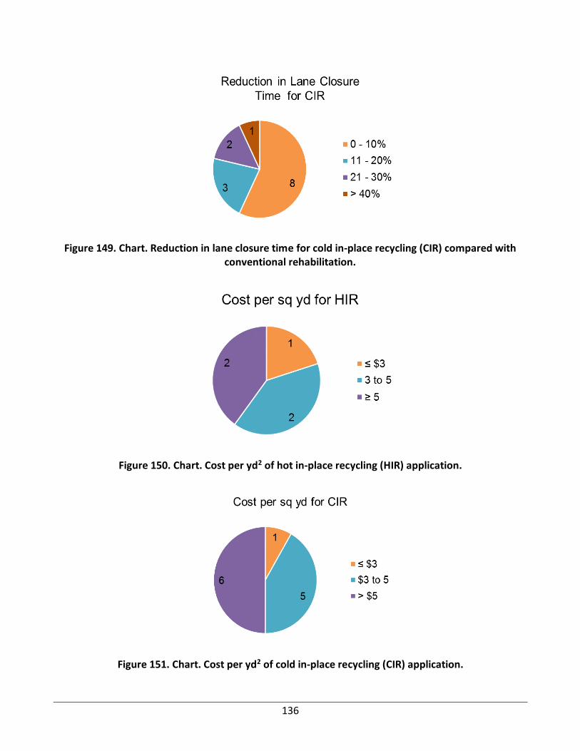
136

Figure 149. Chart. Reduction in lane closure time for cold in-place recycling (CIR) compared with conventional rehabilitation.

Figure 150. Chart. Cost per yd2 of hot in-place recycling (HIR) application.

Figure 151. Chart. Cost per yd2 of cold in-place recycling (CIR) application.

137

APPENDIX B. MAJOR UNIT PROCESSES MODELED

Table 72. Type and Percent Contribution of NERC Regions for Each State

State NERC Region Contribution (%) State NERC Region Contribution (%)

AK ASCC 100 NC SERC 100

AL SERC 100 ND MRO 100

AR SERC 89.6585 NE MRO 100

AR SPP 10.3415 NH NPCC 99.9959

AZ WECC 100 NJ NPCC 6.93202

CA WECC 100 NJ RFC 93.068

CO WECC 100 NM SPP 6.64509

CT NPCC 100 NM WECC 93.3549

DC RFC 100 NV WECC 100

DE RFC 100 NY NPCC 100

FL FRCC 95.5426 OH RFC 99.4508

FL SERC 4.45744 OH TRE 0.549153

GA SERC 100 OK SERC 4.15301

HI HICC 100 OK SPP 90.226

IA MRO 99.1633 OK TRE 5.621

IA RFC 0.836656 OR WECC 100

ID WECC 100 PA RFC 100

IL MRO 0.0255141 RI NPCC 100

IL RFC 65.7789 SC SERC 100

IL SERC 34.1956 SD MRO 99.0926

IN RFC 100 SD WECC 0.907452

KS SPP 100 TN SERC 99.9592

KY RFC 6.77734 TN WECC 0.0408408

KY SERC 93.2227 TX SERC 5.98278

LA SERC 78.1378 TX SPP 10.7096

LA SPP 21.8622 TX TRE 82.6485

MA NPCC 100 TX WECC 0.659124

MD RFC 100 UT WECC 100

ME NPCC 100 VA RFC 2.73803

MI MRO 0.976683 VA SERC 97.262

MI RFC 99.0233 VT NPCC 100

MN MRO 99.9999 WA WECC 100

MO MRO 0.394321 WI MRO 49.9817

MO SERC 66.9628 WI RFC 50.0183

MO SPP 32.6429 WV RFC 88.3757

MS SERC 100 WV SERC 11.6243

MT MRO 6.83667 WY MRO 13.6308

MT WECC 93.1633 WY WECC 86.3692

138

Table 73. Unit Processes Adopted from US-EI 2.2 in Material Stage

Materials Unit Processes from US-EI 2.2

Crushed aggregate Gravel, crushed, at mine/US* US-EI U

Natural aggregate Gravel, round, at mine/US* US-EI U

Sand Sand, at mine/US* US-EI U

Asphalt rejuvenator Paraffin, at plant/US- US-EI U, Benzene, at plant/US- US-EI U

Hydrated lime Lime, hydrated, loose, at plant/US* US-EI U

Table 74. Unit Processes Information of Asphalt Binder Products Used in the Materials Database

Asphalt Binder Product Unit Processes

Emulsion

• 65 percent binder, transported 200 miles by rail

• 1.5 percent hydrochloric acid, transported 200 miles by truck

• 0.2 percent emulsifier (ethylene diamine), transported 200 miles by truck

• 33 kWh (65.32 + 53.5 MJ) electricity

• 83.1 gal water

GTR binder

• 85 percent binder, transported 200 miles by rail

• 15 percent GTR, transported 200 miles by train

• 15.9 kWh electricity

• 6.29E5 KJ heat, light fuel oil, at industrial furnace, US-EI

SBS polymer modified binder

• 96.5 percent binder, transported 200 miles by rail

• 3.5 percent Styrene butadiene rubber, transported 200 miles by truck

• 35.45 ft3 natural gas, combusted in industrial equipment

• 0.0936 gal diesel, combusted in industrial boiler

• 0.0021 tn.sh coal, combusted in industrial boiler

• 54 kWh electricity

Foamed asphalt • 97.5 percent binder, transported 200 miles by rail

• 2.5 percent water

139

APPENDIX C. DECISION MATRIX

Table 75. Decision Matrix (1/3)

Trea

tmen

t Ty

pe

AA

DT

< 50

00

AA

DT

500

0-3

000

0

AA

DT

>300

00

AA

DT

Un

kno

wn

Ru

ral R

oa

d

Urb

an R

oa

d

Ro

ad

Typ

e U

nkn

ow

n

Tru

ck <

10

per

cen

t

Tru

ck>

10 p

erce

nt

Tru

ck V

olu

me

Un

kno

wn

PC

I 86

to

100

PC

I 71

to

85

PC

I 56

to

70

PC

I <5

6

PC

I Un

kno

wn

Low

Rav

elin

g

Med

ium

Rav

elin

g

Hig

h R

avel

ing

Rav

elin

g U

nkn

ow

n

Cape seal 5 5 5 1 5 5 1 5 5 1 5 5 1 1 1 5 5 5 1

Chip seal double course

5 5 1 1 5 5 1 5 5 1 5 5 1 1 1 5 5 5 1

Chip seal single course

0 0 0 1 5 5 1 5 5 1 5 5 1 1 1 5 5 5 1

CIR 5 5 1 1 5 5 1 5 1 1 5 5 5 1 1 5 5 5 1

CIR + cape seal

5 5 1 1 5 5 1 5 1 1 5 5 5 1 1 5 5 5 1

CIR + chip seal

5 5 1 1 5 5 1 5 1 1 5 5 5 1 1 5 5 5 1

CIR + thin overlay (2 inches or less)

5 5 1 1 5 5 1 5 1 1 5 5 5 1 1 5 5 5 1

CIR + medium overlay ( between 2 and 4 inches)

5 5 1 1 5 5 1 5 1 1 5 5 5 1 1 5 5 5 1

CIR + thick overlay (over 4 inches)

5 5 1 1 5 5 1 5 1 1 5 5 5 1 1 5 5 5 1

FDR 5 5 5 1 5 5 1 5 5 1 5 5 5 5 1 5 5 5 1

FDR + cape seal

5 5 5 1 5 5 1 5 5 1 5 5 5 5 1 5 5 5 1 FDR + chip seal

5 5 5 1 5 5 1 5 5 1 5 5 5 5 1 5 5 5 1

FDR + thin overlay (2 inches or less)

5 5 5 1 5 5 1 5 5 1 5 5 5 5 1 5 5 5 1

FDR + medium overlay (between 2 and 4 inches)

5 5 5 1 5 5 1 5 5 1 5 5 5 5 1 5 5 5 1

FDR + thick overlay (over 4 inches)

5 5 5 1 5 5 1 5 5 1 5 5 5 5 1 5 5 5 1

Fog seal 5 5 1 1 5 5 1 5 3 1 5 5 1 1 1 5 5 5 1

HIR remixing

5 5 5 1 5 5 1 5 1 1 5 5 5 1 1 5 5 5 1

HIR remixing + thin overlay (2 inches or less)

5 5 5 1 5 5 1 5 1 1 5 5 5 1 1 5 5 5 1

HIR remixing + medium overlay (between 2 and 4 inches)

5 5 5 1 5 5 1 5 1 1 5 5 5 1 1 5 5 5 1 HIR remixing + thick overlay (over 4 inches)

5 5 5 1 5 5 1 5 1 1 5 5 5 1 1 5 5 5 1

HIR repaving

5 5 5 1 5 5 1 5 1 1 5 5 5 1 1 5 5 5 1

HIR resurfacing

5 5 1 1 5 5 1 5 1 1 5 5 5 1 1 5 5 5 1

140

Trea

tmen

t Ty

pe

AA

DT

< 50

00

AA

DT

500

0-3

000

0

AA

DT

>300

00

AA

DT

Un

kno

wn

Ru

ral R

oa

d

Urb

an R

oa

d

Ro

ad

Typ

e U

nkn

ow

n

Tru

ck <

10

per

cen

t

Tru

ck>

10 p

erce

nt

Tru

ck V

olu

me

Un

kno

wn

PC

I 86

to

100

PC

I 71

to

85

PC

I 56

to

70

PC

I <5

6

PC

I Un

kno

wn

Low

Rav

elin

g

Med

ium

Rav

elin

g

Hig

h R

avel

ing

Rav

elin

g U

nkn

ow

n

HIR resurfacing + thin overlay (2 inches or less)

5 5 1 1 5 5 1 5 1 1 5 5 5 1 1 5 5 5 1

HIR resurfacing + medium overlay (between 2 and 4 inches)

5 5 1 1 5 5 1 5 1 1 5 5 5 1 1 5 5 5 1

HIR resurfacing + thick overlay (over 4 inches)

5 5 1 1 5 5 1 5 1 1 5 5 5 1 1 5 5 5 1

Microsurfacing double course

0 0 0 1 5 5 1 5 5 1 5 5 1 1 1 5 5 5 1

Microsurfacing single course

5 5 5 1 5 5 1 5 5 1 5 5 1 1 1 5 5 5 1

Cold Milling + Thin Overlay (2 inches or less)

5 5 5 1 5 5 1 5 5 1 5 5 5 1 1 5 5 5 1


5 5 5 1 5 5 1 5 5 1 5 5 5 1 1 5 5 5 1

Cold Milling + Thick Overlay (over 4 inches)

5 5 5 1 5 5 1 5 5 1 5 5 5 5 1 5 5 5 1

Sand seal 5 5 1 1 5 3 1 5 3 1 5 5 1 1 1 5 5 5 1

Slurry seal 5 5 5 1 1 5 1 5 3 1 5 5 1 1 1 5 5 5 1

Thin HMA Overlay (2 inches or less)

5 5 5 1 5 5 1 5 5 1 5 5 5 1 1 5 5 5 1

Ultra thin bonded wearing course

5 5 5 1 5 5 1 5 5 1 5 5 5 1 1 5 5 5 1

141

Table 76. Decision Matrix (2/3) Tr

eatm

ent

Typ

e

Low

Po

tho

les

Med

ium

Po

tho

les

Hig

h P

oth

ole

s

Po

tho

les

Un

kno

wn

Ble

edin

g

No

Ble

edin

g

Ble

edin

g U

nkn

ow

n

Low

Ski

d R

esis

tan

ce

Hig

h S

kid

Res

ista

nce

Skid

Res

ista

nce

Un

kno

wn

Sho

uld

er D

rop

-Off

No

Sh

ou

lder

Dro

p-O

ff

Sho

uld

er D

rop

-off

Un

kno

wn

Low

Ru

ttin

g

Med

ium

Ru

ttin

g

Hig

h R

utt

ing

Ru

ttin

g U

nkn

ow

n

Low

Co

rru

gati

on

s

Med

ium

Co

rru

gati

on

s

Hig

h C

orr

uga

tio

ns

Co

rru

gati

on

s U

nkn

ow

n

Low

Fat

igu

e

Med

ium

Fat

igu

e

Hig

h F

atig

ue

Fati

gue

Un

kno

wn

Cape seal

5 3 3 1 1 5 1 5 5 1 1 5 1 4 3 1 1 3 3 1 1 3 3 1 1


5 3 1 1 1 5 1 5 5 1 1 5 1 4 3 1 1 3 3 1 1 3 3 1 1


5 3 1 1 1 5 1 5 5 1 1 5 1 4 1 1 1 4 3 1 1 3 3 1 1

CIR 5 5 5 1 3 5 1 5 5 1 1 5 1 4 5 5 1 4 5 5 1 5 4 4 1

CIR + cape seal

5 5 5 1 3 5 1 5 5 1 1 5 1 4 5 5 1 4 5 5 1 5 4 4 1

CIR + chip seal

5 5 5 1 3 5 1 5 5 1 1 5 1 4 5 5 1 4 5 5 1 5 4 4 1

142

Trea

tmen

t Ty

pe

Low

Po

tho

les

Med

ium

Po

tho

les

Hig

h P

oth

ole

s

Po

tho

les

Un

kno

wn

Ble

edin

g

No

Ble

edin

g

Ble

edin

g U

nkn

ow

n

Low

Ski

d R

esis

tan

ce

Hig

h S

kid

Res

ista

nce

Skid

Res

ista

nce

Un

kno

wn

Sho

uld

er D

rop

-Off

No

Sh

ou

lder

Dro

p-O

ff

Sho

uld

er D

rop

-off

Un

kno

wn

Low

Ru

ttin

g

Med

ium

Ru

ttin

g

Hig

h R

utt

ing

Ru

ttin

g U

nkn

ow

n

Low

Co

rru

gati

on

s

Med

ium

Co

rru

gati

on

s

Hig

h C

orr

uga

tio

ns

Co

rru

gati

on

s U

nkn

ow

n

Low

Fat

igu

e

Med

ium

Fat

igu

e

Hig

h F

atig

ue

Fati

gue

Un

kno

wn


5 5 5 1 3 5 1 5 5 1 1 5 1 4 5 5 1 4 5 5 1 5 4 4 1


5 5 5 1 3 5 1 5 5 1 1 5 1 4 5 5 1 4 5 5 1 5 4 4 1


5 5 5 1 3 5 1 5 5 1 1 5 1 4 5 5 1 4 5 5 1 5 4 4 1

FDR 5 5 5 1 5 5 1 5 5 1 1 5 1 5 5 5 1 5 5 5 1 5 5 5 1

143

Trea

tmen

t Ty

pe

Low

Po

tho

les

Med

ium

Po

tho

les

Hig

h P

oth

ole

s

Po

tho

les

Un

kno

wn

Ble

edin

g

No

Ble

edin

g

Ble

edin

g U

nkn

ow

n

Low

Ski

d R

esis

tan

ce

Hig

h S

kid

Res

ista

nce

Skid

Res

ista

nce

Un

kno

wn

Sho

uld

er D

rop

-Off

No

Sh

ou

lder

Dro

p-O

ff

Sho

uld

er D

rop

-off

Un

kno

wn

Low

Ru

ttin

g

Med

ium

Ru

ttin

g

Hig

h R

utt

ing

Ru

ttin

g U

nkn

ow

n

Low

Co

rru

gati

on

s

Med

ium

Co

rru

gati

on

s

Hig

h C

orr

uga

tio

ns

Co

rru

gati

on

s U

nkn

ow

n

Low

Fat

igu

e

Med

ium

Fat

igu

e

Hig

h F

atig

ue

Fati

gue

Un

kno

wn

FDR + cape seal

5 5 5 1 5 5 1 5 5 1 1 5 1 5 5 5 1 5 5 5 1 5 5 5 1

FDR + chip seal

5 5 5 1 5 5 1 5 5 1 1 5 1 5 5 5 1 5 5 5 1 5 5 5 1

FDR + thin overlay (2 inches or less)

5 5 5 1 5 5 1 5 5 1 1 5 1 5 5 5 1 5 5 5 1 5 5 5 1


5 5 5 1 5 5 1 5 5 1 1 5 1 5 5 5 1 5 5 5 1 5 5 5 1

144

Trea

tmen

t Ty

pe

Low

Po

tho

les

Med

ium

Po

tho

les

Hig

h P

oth

ole

s

Po

tho

les

Un

kno

wn

Ble

edin

g

No

Ble

edin

g

Ble

edin

g U

nkn

ow

n

Low

Ski

d R

esis

tan

ce

Hig

h S

kid

Res

ista

nce

Skid

Res

ista

nce

Un

kno

wn

Sho

uld

er D

rop

-Off

No

Sh

ou

lder

Dro

p-O

ff

Sho

uld

er D

rop

-off

Un

kno

wn

Low

Ru

ttin

g

Med

ium

Ru

ttin

g

Hig

h R

utt

ing

Ru

ttin

g U

nkn

ow

n

Low

Co

rru

gati

on

s

Med

ium

Co

rru

gati

on

s

Hig

h C

orr

uga

tio

ns

Co

rru

gati

on

s U

nkn

ow

n

Low

Fat

igu

e

Med

ium

Fat

igu

e

Hig

h F

atig

ue

Fati

gue

Un

kno

wn


5 5 5 1 5 5 1 5 5 1 1 5 1 5 5 5 1 5 5 5 1 5 5 5 1

Fog seal

1 1 1 1 1 5 1 1 5 1 1 5 1 1 1 1 1 1 1 1 1 1 1 1 1

HIR remixing

5 5 3 1 3 5 1 5 5 1 1 5 1 0 0 0 1 4 5 5 1 5 4 4 1

HIR remixing + thin overlay (2 inches or less)

5 5 3 1 3 5 1 5 5 1 1 5 1 4 5 5 1 4 5 5 1 5 4 4 1

HIR remixing +

5 5 3 1 3 5 1 5 5 1 1 5 1 4 5 5 1 4 5 5 1 5 4 4 1

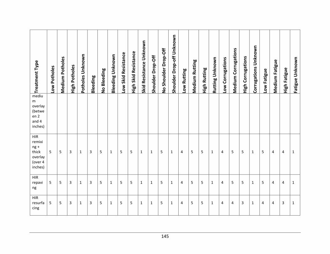
145

Trea

tmen

t Ty

pe

Low

Po

tho

les

Med

ium

Po

tho

les

Hig

h P

oth

ole

s

Po

tho

les

Un

kno

wn

Ble

edin

g

No

Ble

edin

g

Ble

edin

g U

nkn

ow

n

Low

Ski

d R

esis

tan

ce

Hig

h S

kid

Res

ista

nce

Skid

Res

ista

nce

Un

kno

wn

Sho

uld

er D

rop

-Off

No

Sh

ou

lder

Dro

p-O

ff

Sho

uld

er D

rop

-off

Un

kno

wn

Low

Ru

ttin

g

Med

ium

Ru

ttin

g

Hig

h R

utt

ing

Ru

ttin

g U

nkn

ow

n

Low

Co

rru

gati

on

s

Med

ium

Co

rru

gati

on

s

Hig

h C

orr

uga

tio

ns

Co

rru

gati

on

s U

nkn

ow

n

Low

Fat

igu

e

Med

ium

Fat

igu

e

Hig

h F

atig

ue

Fati

gue

Un

kno

wn

medium overlay (between 2 and 4 inches)

HIR remixing + thick overlay (over 4 inches)

5 5 3 1 3 5 1 5 5 1 1 5 1 4 5 5 1 4 5 5 1 5 4 4 1

HIR repaving

5 5 3 1 3 5 1 5 5 1 1 5 1 4 5 5 1 4 5 5 1 5 4 4 1

HIR resurfacing

5 5 3 1 3 5 1 5 5 1 1 5 1 4 5 5 1 4 4 3 1 4 4 3 1

146

Trea

tmen

t Ty

pe

Low

Po

tho

les

Med

ium

Po

tho

les

Hig

h P

oth

ole

s

Po

tho

les

Un

kno

wn

Ble

edin

g

No

Ble

edin

g

Ble

edin

g U

nkn

ow

n

Low

Ski

d R

esis

tan

ce

Hig

h S

kid

Res

ista

nce

Skid

Res

ista

nce

Un

kno

wn

Sho

uld

er D

rop

-Off

No

Sh

ou

lder

Dro

p-O

ff

Sho

uld

er D

rop

-off

Un

kno

wn

Low

Ru

ttin

g

Med

ium

Ru

ttin

g

Hig

h R

utt

ing

Ru

ttin

g U

nkn

ow

n

Low

Co

rru

gati

on

s

Med

ium

Co

rru

gati

on

s

Hig

h C

orr

uga

tio

ns

Co

rru

gati

on

s U

nkn

ow

n

Low

Fat

igu

e

Med

ium

Fat

igu

e

Hig

h F

atig

ue

Fati

gue

Un

kno

wn


5 5 3 1 3 5 1 5 5 1 1 5 1 4 5 5 1 5 4 3 1 4 4 3 1


5 5 3 1 3 5 1 5 5 1 1 5 1 4 5 5 1 5 4 3 1 4 4 3 1

HIR resurfacing + thick overlay

5 5 3 1 3 5 1 5 5 1 1 5 1 4 5 5 1 5 4 3 1 4 4 3 1

147

Trea

tmen

t Ty

pe

Low

Po

tho

les

Med

ium

Po

tho

les

Hig

h P

oth

ole

s

Po

tho

les

Un

kno

wn

Ble

edin

g

No

Ble

edin

g

Ble

edin

g U

nkn

ow

n

Low

Ski

d R

esis

tan

ce

Hig

h S

kid

Res

ista

nce

Skid

Res

ista

nce

Un

kno

wn

Sho

uld

er D

rop

-Off

No

Sh

ou

lder

Dro

p-O

ff

Sho

uld

er D

rop

-off

Un

kno

wn

Low

Ru

ttin

g

Med

ium

Ru

ttin

g

Hig

h R

utt

ing

Ru

ttin

g U

nkn

ow

n

Low

Co

rru

gati

on

s

Med

ium

Co

rru

gati

on

s

Hig

h C

orr

uga

tio

ns

Co

rru

gati

on

s U

nkn

ow

n

Low

Fat

igu

e

Med

ium

Fat

igu

e

Hig

h F

atig

ue

Fati

gue

Un

kno

wn

(over 4 inches)


5 3 3 1 1 5 1 5 5 1 1 5 1 5 4 3 1 3 3 1 1 3 3 1 1


5 3 3 1 1 5 1 5 5 1 1 5 1 4 3 1 1 3 1 1 1 3 3 1 1


5 5 5 1 3 5 1 5 5 1 1 5 1 4 5 4 1 5 5 5 1 4 4 3 1

Cold Milling

5 5 5 1 3 5 1 5 5 1 1 5 1 5 5 5 1 5 5 5 1 4 4 4 1

148

Trea

tmen

t Ty

pe

Low

Po

tho

les

Med

ium

Po

tho

les

Hig

h P

oth

ole

s

Po

tho

les

Un

kno

wn

Ble

edin

g

No

Ble

edin

g

Ble

edin

g U

nkn

ow

n

Low

Ski

d R

esis

tan

ce

Hig

h S

kid

Res

ista

nce

Skid

Res

ista

nce

Un

kno

wn

Sho

uld

er D

rop

-Off

No

Sh

ou

lder

Dro

p-O

ff

Sho

uld

er D

rop

-off

Un

kno

wn

Low

Ru

ttin

g

Med

ium

Ru

ttin

g

Hig

h R

utt

ing

Ru

ttin

g U

nkn

ow

n

Low

Co

rru

gati

on

s

Med

ium

Co

rru

gati

on

s

Hig

h C

orr

uga

tio

ns

Co

rru

gati

on

s U

nkn

ow

n

Low

Fat

igu

e

Med

ium

Fat

igu

e

Hig

h F

atig

ue

Fati

gue

Un

kno

wn

+ Medium Overlay (between 2 and 4 inches)


5 5 5 1 3 5 1 5 5 1 1 5 1 5 5 5 1 5 5 5 1 4 4 4 1

Sand seal

5 3 1 1 0 0 1 5 5 1 1 5 1 1 1 1 1 1 1 1 1 1 1 1 1

Slurry seal

5 3 3 1 1 5 1 5 5 1 1 5 1 3 1 1 1 1 1 1 1 1 1 1 1

149

Trea

tmen

t Ty

pe

Low

Po

tho

les

Med

ium

Po

tho

les

Hig

h P

oth

ole

s

Po

tho

les

Un

kno

wn

Ble

edin

g

No

Ble

edin

g

Ble

edin

g U

nkn

ow

n

Low

Ski

d R

esis

tan

ce

Hig

h S

kid

Res

ista

nce

Skid

Res

ista

nce

Un

kno

wn

Sho

uld

er D

rop

-Off

No

Sh

ou

lder

Dro

p-O

ff

Sho

uld

er D

rop

-off

Un

kno

wn

Low

Ru

ttin

g

Med

ium

Ru

ttin

g

Hig

h R

utt

ing

Ru

ttin

g U

nkn

ow

n

Low

Co

rru

gati

on

s

Med

ium

Co

rru

gati

on

s

Hig

h C

orr

uga

tio

ns

Co

rru

gati

on

s U

nkn

ow

n

Low

Fat

igu

e

Med

ium

Fat

igu

e

Hig

h F

atig

ue

Fati

gue

Un

kno

wn


5 5 5 1 3 5 1 5 5 1 1 5 1 4 5 4 1 5 4 3 1 5 5 3 1


5 1 1 1 1 5 1 5 5 1 1 5 1 4 3 1 1 4 3 1 1 3 3 1 1

150

Table 77. Decision Matrix (3/3)

Tre

atm

en

t Ty

pe

Low

Ed

ge C

rack

ing

Me

diu

m E

dge

Cra

ckin

g

Hig

h E

dge

Cra

ckin

g

Edge

Cra

ckin

g

Low

Slip

pag

e

Me

diu

m S

lipp

age

Hig

h S

lipp

age

Slip

pag

e U

nkn

ow

n

Low

Blo

ck C

rack

ing

Me

diu

m B

lock

Cra

ckin

g

Hig

h B

lock

Cra

ckin

g

Blo

ck C

rack

ing

Un

kno

wn

Low

Lo

ngi

tud

inal

Cra

ckin

g

Me

diu

m L

on

gitu

din

al C

rack

ing

Hig

h L

on

gitu

din

al C

rack

ing

Lon

gitu

din

al C

rack

ing

Un

kno

wn

Low

Tra

nsv

ers

e C

rack

ing

Me

diu

m T

ran

sve

rse

Cra

ckin

g

Hig

h T

ran

sve

rse

Cra

ckin

g

Tran

sve

rse

Cra

ckin

g U

nkn

ow

n

Cape seal 3 3 1 1 3 3 1 1 5 3 1 1 3 3 1 1 5 3 1 1


4 4 3 1 3 3 1 1 5 4 3 1 4 4 3 1 5 4 3 1


5 4 4 1 3 3 1 1 5 4 4 1 5 4 4 1 5 4 4 1

CIR 5 3 1 1 5 4 4 1 5 5 4 1 5 3 1 1 3 3 1 1

CIR + cape seal

5 3 1 1 5 4 4 1 5 5 4 1 5 3 1 1 3 3 1 1

CIR + chip seal

5 3 1 1 5 4 4 1 5 5 4 1 5 3 1 1 3 3 1 1


5 3 1 1 5 4 4 1 5 5 4 1 5 3 1 1 3 3 1 1

151

Tre

atm

en

t Ty

pe

Low

Ed

ge C

rack

ing

Me

diu

m E

dge

Cra

ckin

g

Hig

h E

dge

Cra

ckin

g

Edge

Cra

ckin

g

Low

Slip

pag

e

Me

diu

m S

lipp

age

Hig

h S

lipp

age

Slip

pag

e U

nkn

ow

n

Low

Blo

ck C

rack

ing

Me

diu

m B

lock

Cra

ckin

g

Hig

h B

lock

Cra

ckin

g

Blo

ck C

rack

ing

Un

kno

wn

Low

Lo

ngi

tud

inal

Cra

ckin

g

Me

diu

m L

on

gitu

din

al C

rack

ing

Hig

h L

on

gitu

din

al C

rack

ing

Lon

gitu

din

al C

rack

ing

Un

kno

wn

Low

Tra

nsv

ers

e C

rack

ing

Me

diu

m T

ran

sve

rse

Cra

ckin

g

Hig

h T

ran

sve

rse

Cra

ckin

g

Tran

sve

rse

Cra

ckin

g U

nkn

ow

n


5 3 1 1 5 4 4 1 5 5 4 1 5 3 1 1 3 3 1 1


5 3 1 1 5 4 4 1 5 5 4 1 5 3 1 1 3 3 1 1

FDR 5 5 5 1 5 5 5 1 5 5 5 1 5 5 5 1 5 5 5 1

FDR + cape seal

5 5 5 1 5 5 5 1 5 5 5 1 5 5 5 1 5 5 5 1

FDR + chip seal

5 5 5 1 5 5 5 1 5 5 5 1 5 5 5 1 5 5 5 1

FDR + thin overlay (2

5 5 5 1 5 5 5 1 5 5 5 1 5 5 5 1 5 5 5 1

152

Tre

atm

en

t Ty

pe

Low

Ed

ge C

rack

ing

Me

diu

m E

dge

Cra

ckin

g

Hig

h E

dge

Cra

ckin

g

Edge

Cra

ckin

g

Low

Slip

pag

e

Me

diu

m S

lipp

age

Hig

h S

lipp

age

Slip

pag

e U

nkn

ow

n

Low

Blo

ck C

rack

ing

Me

diu

m B

lock

Cra

ckin

g

Hig

h B

lock

Cra

ckin

g

Blo

ck C

rack

ing

Un

kno

wn

Low

Lo

ngi

tud

inal

Cra

ckin

g

Me

diu

m L

on

gitu

din

al C

rack

ing

Hig

h L

on

gitu

din

al C

rack

ing

Lon

gitu

din

al C

rack

ing

Un

kno

wn

Low

Tra

nsv

ers

e C

rack

ing

Me

diu

m T

ran

sve

rse

Cra

ckin

g

Hig

h T

ran

sve

rse

Cra

ckin

g

Tran

sve

rse

Cra

ckin

g U

nkn

ow

n

inches or less)


5 5 5 1 5 5 5 1 5 5 5 1 5 5 5 1 5 5 5 1


5 5 5 1 5 5 5 1 5 5 5 1 5 5 5 1 5 5 5 1

Fog seal 3 1 1 1 1 1 1 1 3 1 1 1 3 1 1 1 3 1 1 1

HIR remixing

5 3 1 1 5 4 4 1 5 4 4 1 5 3 1 1 3 3 1 1

HIR remixing + thin

5 3 1 1 5 4 4 1 5 4 4 1 5 3 1 1 3 3 1 1

153

Tre

atm

en

t Ty

pe

Low

Ed

ge C

rack

ing

Me

diu

m E

dge

Cra

ckin

g

Hig

h E

dge

Cra

ckin

g

Edge

Cra

ckin

g

Low

Slip

pag

e

Me

diu

m S

lipp

age

Hig

h S

lipp

age

Slip

pag

e U

nkn

ow

n

Low

Blo

ck C

rack

ing

Me

diu

m B

lock

Cra

ckin

g

Hig

h B

lock

Cra

ckin

g

Blo

ck C

rack

ing

Un

kno

wn

Low

Lo

ngi

tud

inal

Cra

ckin

g

Me

diu

m L

on

gitu

din

al C

rack

ing

Hig

h L

on

gitu

din

al C

rack

ing

Lon

gitu

din

al C

rack

ing

Un

kno

wn

Low

Tra

nsv

ers

e C

rack

ing

Me

diu

m T

ran

sve

rse

Cra

ckin

g

Hig

h T

ran

sve

rse

Cra

ckin

g

Tran

sve

rse

Cra

ckin

g U

nkn

ow

n

overlay (2 inches or less)


5 3 1 1 5 4 4 1 5 4 4 1 5 3 1 1 3 3 1 1


5 3 1 1 5 4 4 1 5 4 4 1 5 3 1 1 3 3 1 1

HIR repaving

5 3 1 1 5 4 4 1 5 4 4 1 5 3 1 1 3 3 1 1

154

Tre

atm

en

t Ty

pe

Low

Ed

ge C

rack

ing

Me

diu

m E

dge

Cra

ckin

g

Hig

h E

dge

Cra

ckin

g

Edge

Cra

ckin

g

Low

Slip

pag

e

Me

diu

m S

lipp

age

Hig

h S

lipp

age

Slip

pag

e U

nkn

ow

n

Low

Blo

ck C

rack

ing

Me

diu

m B

lock

Cra

ckin

g

Hig

h B

lock

Cra

ckin

g

Blo

ck C

rack

ing

Un

kno

wn

Low

Lo

ngi

tud

inal

Cra

ckin

g

Me

diu

m L

on

gitu

din

al C

rack

ing

Hig

h L

on

gitu

din

al C

rack

ing

Lon

gitu

din

al C

rack

ing

Un

kno

wn

Low

Tra

nsv

ers

e C

rack

ing

Me

diu

m T

ran

sve

rse

Cra

ckin

g

Hig

h T

ran

sve

rse

Cra

ckin

g

Tran

sve

rse

Cra

ckin

g U

nkn

ow

n

HIR resurfacing

5 3 1 1 4 4 3 1 5 4 3 1 5 3 1 1 3 3 1 1


5 3 1 1 4 4 3 1 5 4 3 1 5 3 1 1 3 3 1 1


5 3 1 1 4 4 3 1 5 4 3 1 5 3 1 1 3 3 1 1

HIR resurfacing + thick overlay

5 3 1 1 4 4 3 1 5 4 3 1 5 3 1 1 3 3 1 1

155

Tre

atm

en

t Ty

pe

Low

Ed

ge C

rack

ing

Me

diu

m E

dge

Cra

ckin

g

Hig

h E

dge

Cra

ckin

g

Edge

Cra

ckin

g

Low

Slip

pag

e

Me

diu

m S

lipp

age

Hig

h S

lipp

age

Slip

pag

e U

nkn

ow

n

Low

Blo

ck C

rack

ing

Me

diu

m B

lock

Cra

ckin

g

Hig

h B

lock

Cra

ckin

g

Blo

ck C

rack

ing

Un

kno

wn

Low

Lo

ngi

tud

inal

Cra

ckin

g

Me

diu

m L

on

gitu

din

al C

rack

ing

Hig

h L

on

gitu

din

al C

rack

ing

Lon

gitu

din

al C

rack

ing

Un

kno

wn

Low

Tra

nsv

ers

e C

rack

ing

Me

diu

m T

ran

sve

rse

Cra

ckin

g

Hig

h T

ran

sve

rse

Cra

ckin

g

Tran

sve

rse

Cra

ckin

g U

nkn

ow

n

(over 4 inches )


5 4 3 1 3 3 1 1 5 3 1 1 5 4 3 1 5 4 3 1


4 3 1 1 3 3 1 1 5 3 1 1 4 3 1 1 5 3 1 1


5 3 1 1 4 4 3 1 5 5 4 1 5 3 1 1 5 3 1 1

Cold Milling + Medium Overlay

5 4 4 1 4 4 4 1 5 5 4 1 5 4 4 1 5 3 3 1

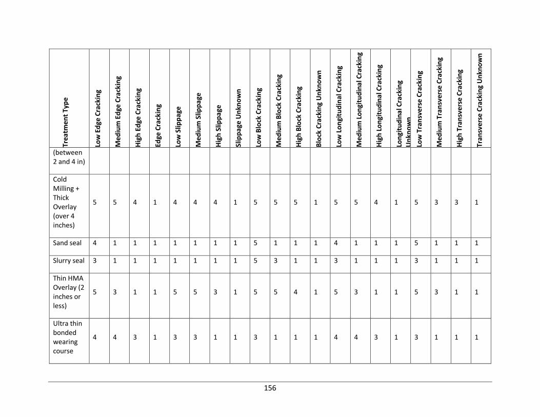
156

Tre

atm

en

t Ty

pe

Low

Ed

ge C

rack

ing

Me

diu

m E

dge

Cra

ckin

g

Hig

h E

dge

Cra

ckin

g

Edge

Cra

ckin

g

Low

Slip

pag

e

Me

diu

m S

lipp

age

Hig

h S

lipp

age

Slip

pag

e U

nkn

ow

n

Low

Blo

ck C

rack

ing

Me

diu

m B

lock

Cra

ckin

g

Hig

h B

lock

Cra

ckin

g

Blo

ck C

rack

ing

Un

kno

wn

Low

Lo

ngi

tud

inal

Cra

ckin

g

Me

diu

m L

on

gitu

din

al C

rack

ing

Hig

h L

on

gitu

din

al C

rack

ing

Lon

gitu

din

al C

rack

ing

Un

kno

wn

Low

Tra

nsv

ers

e C

rack

ing

Me

diu

m T

ran

sve

rse

Cra

ckin

g

Hig

h T

ran

sve

rse

Cra

ckin

g

Tran

sve

rse

Cra

ckin

g U

nkn

ow

n

(between 2 and 4 in)


5 5 4 1 4 4 4 1 5 5 5 1 5 5 4 1 5 3 3 1

Sand seal 4 1 1 1 1 1 1 1 5 1 1 1 4 1 1 1 5 1 1 1

Slurry seal 3 1 1 1 1 1 1 1 5 3 1 1 3 1 1 1 3 1 1 1


5 3 1 1 5 5 3 1 5 5 4 1 5 3 1 1 5 3 1 1


4 4 3 1 3 3 1 1 3 1 1 1 4 4 3 1 3 1 1 1

157

Trea

tmen

t Ty

pe

Ro

ugh

Rid

e Q

ual

ity

No

t R

ou

gh R

ide

Qu

alit

y

Ro

ugh

Rid

e Q

ual

ity

Un

kno

wn

Ad

equ

ate

Dra

inag

e

No

t A

deq

uat

e D

rain

age

Dra

inag

e U

nkn

ow

n

CB

R<3

CB

R 3

-10

CB

R>1

0

CB

R U

nkn

ow

n

Mix

Des

ign

Per

form

ed

Mix

Des

ign

No

t P

erfo

rmed

Mix

Des

ign

Un

kno

wn

Dry

-Co

ld C

limat

e

Wet

-Co

ld C

limat

e

Wet

-Ho

t C

limat

e

Wet

-Ho

t C

limat

e

Dry

-Ho

t C

limat

e

Clim

ate

Un

kno

wn

Clim

ate

Un

kno

wn

Cape seal 3 5 1 5 1 1 1 1 5 1 5 1 1 0 0 0 0 0


3 5 1 5 1 1 1 1 5 1 5 1 1 5 5 5 5 1


3 5 1 5 1 1 1 1 5 1 5 1 1 5 3 3 3 1

CIR 5 5 1 5 1 1 1 1 5 1 5 1 1 5 3 3 5 1

CIR + cape seal

5 5 1 5 1 1 1 1 5 1 5 1 1 5 3 3 5 1

CIR + chip seal

5 5 1 5 1 1 1 1 5 1 5 1 1 5 3 3 5 1


5 5 1 5 1 1 1 1 5 1 5 1 1 5 3 3 5 1

158

Trea

tmen

t Ty

pe

Ro

ugh

Rid

e Q

ual

ity

No

t R

ou

gh R

ide

Qu

alit

y

Ro

ugh

Rid

e Q

ual

ity

Un

kno

wn

Ad

equ

ate

Dra

inag

e

No

t A

deq

uat

e D

rain

age

Dra

inag

e U

nkn

ow

n

CB

R<3

CB

R 3

-10

CB

R>1

0

CB

R U

nkn

ow

n

Mix

Des

ign

Per

form

ed

Mix

Des

ign

No

t P

erfo

rmed

Mix

Des

ign

Un

kno

wn

Dry

-Co

ld C

limat

e

Wet

-Co

ld C

limat

e

Wet

-Ho

t C

limat

e

Wet

-Ho

t C

limat

e

Dry

-Ho

t C

limat

e

Clim

ate

Un

kno

wn

Clim

ate

Un

kno

wn


5 5 1 5 1 1 1 1 5 1 5 1 1 5 3 3 5 1


5 5 1 5 1 1 1 1 5 1 5 1 1 5 3 3 5 1

FDR 5 5 1 5 1 1 5 5 5 1 5 1 1 5 5 5 5 1

FDR + cape seal

5 5 1 5 1 1 5 5 5 1 5 1 1 5 5 5 5 1

FDR + chip seal

5 5 1 5 1 1 5 5 5 1 5 1 1 5 5 5 5 1

FDR + thin overlay (2

5 5 1 5 1 1 5 5 5 1 5 1 1 5 5 5 5 1

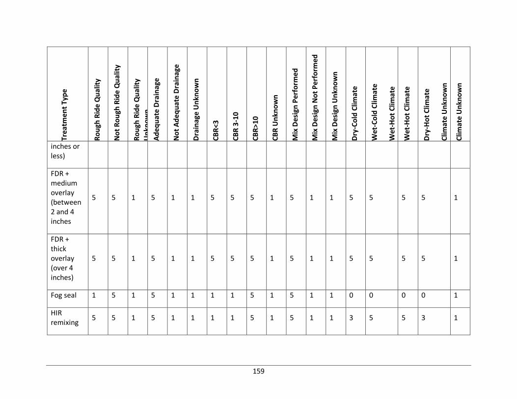
159

Trea

tmen

t Ty

pe

Ro

ugh

Rid

e Q

ual

ity

No

t R

ou

gh R

ide

Qu

alit

y

Ro

ugh

Rid

e Q

ual

ity

Un

kno

wn

Ad

equ

ate

Dra

inag

e

No

t A

deq

uat

e D

rain

age

Dra

inag

e U

nkn

ow

n

CB

R<3

CB

R 3

-10

CB

R>1

0

CB

R U

nkn

ow

n

Mix

Des

ign

Per

form

ed

Mix

Des

ign

No

t P

erfo

rmed

Mix

Des

ign

Un

kno

wn

Dry

-Co

ld C

limat

e

Wet

-Co

ld C

limat

e

Wet

-Ho

t C

limat

e

Wet

-Ho

t C

limat

e

Dry

-Ho

t C

limat

e

Clim

ate

Un

kno

wn

Clim

ate

Un

kno

wn

inches or less)

FDR + medium overlay (between 2 and 4 inches

5 5 1 5 1 1 5 5 5 1 5 1 1 5 5 5 5 1


5 5 1 5 1 1 5 5 5 1 5 1 1 5 5 5 5 1

Fog seal 1 5 1 5 1 1 1 1 5 1 5 1 1 0 0 0 0 1

HIR remixing

5 5 1 5 1 1 1 1 5 1 5 1 1 3 5 5 3 1

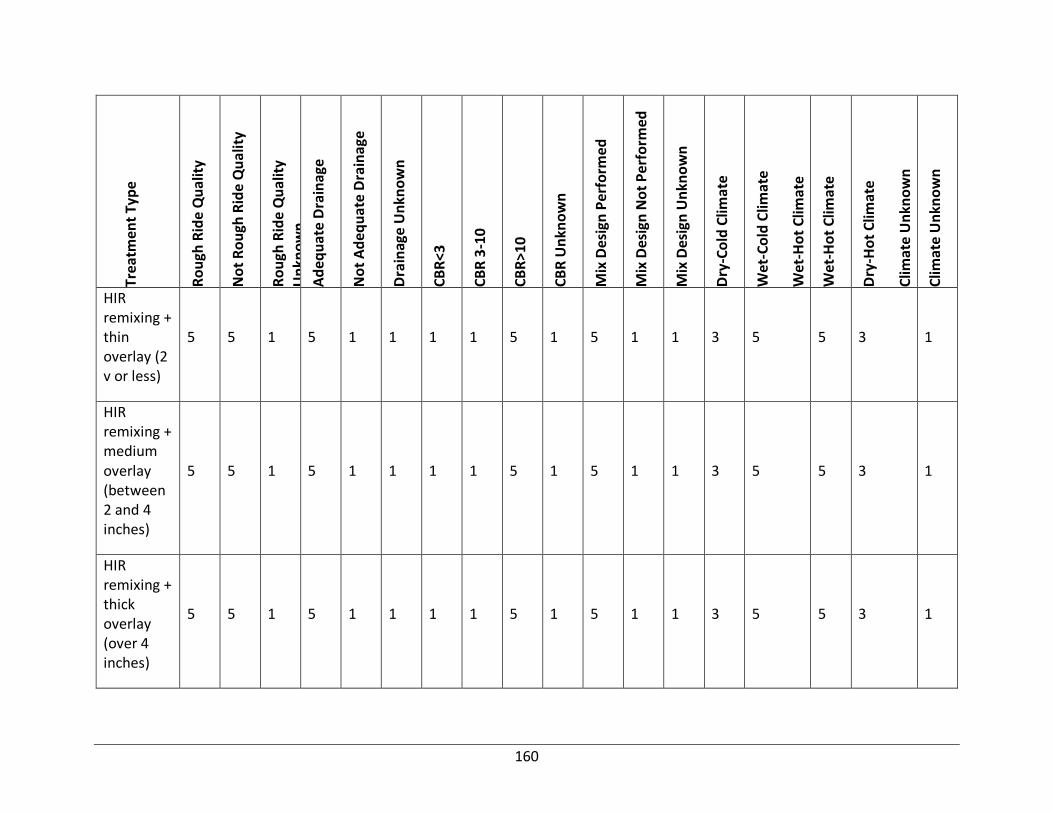
160

Trea

tmen

t Ty

pe

Ro

ugh

Rid

e Q

ual

ity

No

t R

ou

gh R

ide

Qu

alit

y

Ro

ugh

Rid

e Q

ual

ity

Un

kno

wn

Ad

equ

ate

Dra

inag

e

No

t A

deq

uat

e D

rain

age

Dra

inag

e U

nkn

ow

n

CB

R<3

CB

R 3

-10

CB

R>1

0

CB

R U

nkn

ow

n

Mix

Des

ign

Per

form

ed

Mix

Des

ign

No

t P

erfo

rmed

Mix

Des

ign

Un

kno

wn

Dry

-Co

ld C

limat

e

Wet

-Co

ld C

limat

e

Wet

-Ho

t C

limat

e

Wet

-Ho

t C

limat

e

Dry

-Ho

t C

limat

e

Clim

ate

Un

kno

wn

Clim

ate

Un

kno

wn

HIR remixing + thin overlay (2 v or less)

5 5 1 5 1 1 1 1 5 1 5 1 1 3 5 5 3 1


5 5 1 5 1 1 1 1 5 1 5 1 1 3 5 5 3 1


5 5 1 5 1 1 1 1 5 1 5 1 1 3 5 5 3 1

161

Trea

tmen

t Ty

pe

Ro

ugh

Rid

e Q

ual

ity

No

t R

ou

gh R

ide

Qu

alit

y

Ro

ugh

Rid

e Q

ual

ity

Un

kno

wn

Ad

equ

ate

Dra

inag

e

No

t A

deq

uat

e D

rain

age

Dra

inag

e U

nkn

ow

n

CB

R<3

CB

R 3

-10

CB

R>1

0

CB

R U

nkn

ow

n

Mix

Des

ign

Per

form

ed

Mix

Des

ign

No

t P

erfo

rmed

Mix

Des

ign

Un

kno

wn

Dry

-Co

ld C

limat

e

Wet

-Co

ld C

limat

e

Wet

-Ho

t C

limat

e

Wet

-Ho

t C

limat

e

Dry

-Ho

t C

limat

e

Clim

ate

Un

kno

wn

Clim

ate

Un

kno

wn

HIR repaving

5 5 1 5 1 1 1 1 5 1 5 1 1 3 5 5 3 1

HIR resurfacing

5 5 1 5 1 1 1 1 5 1 5 1 1 3 5 5 3 1


5 5 1 5 1 1 1 1 5 1 5 1 1 3 5 5 3 1

HIR resurfacing + medium overlay (between

5 5 1 5 1 1 1 1 5 1 5 1 1 3 5 5 3 1

162

Trea

tmen

t Ty

pe

Ro

ugh

Rid

e Q

ual

ity

No

t R

ou

gh R

ide

Qu

alit

y

Ro

ugh

Rid

e Q

ual

ity

Un

kno

wn

Ad

equ

ate

Dra

inag

e

No

t A

deq

uat

e D

rain

age

Dra

inag

e U

nkn

ow

n

CB

R<3

CB

R 3

-10

CB

R>1

0

CB

R U

nkn

ow

n

Mix

Des

ign

Per

form

ed

Mix

Des

ign

No

t P

erfo

rmed

Mix

Des

ign

Un

kno

wn

Dry

-Co

ld C

limat

e

Wet

-Co

ld C

limat

e

Wet

-Ho

t C

limat

e

Wet

-Ho

t C

limat

e

Dry

-Ho

t C

limat

e

Clim

ate

Un

kno

wn

Clim

ate

Un

kno

wn

2 and 4 inches)

HIR resurfacing + thick overlay (over 4 inches)

5 5 1 5 1 1 1 1 5 1 5 1 1 3 5 5 3 1


3 5 1 5 1 1 1 1 5 1 5 1 1 5 5 5 3 1


3 5 1 5 1 1 1 1 5 1 5 1 1 5 5 5 5 1

Cold Milling +

5 5 1 5 1 1 1 1 5 1 5 1 1 5 5 5 5 1

163

Trea

tmen

t Ty

pe

Ro

ugh

Rid

e Q

ual

ity

No

t R

ou

gh R

ide

Qu

alit

y

Ro

ugh

Rid

e Q

ual

ity

Un

kno

wn

Ad

equ

ate

Dra

inag

e

No

t A

deq

uat

e D

rain

age

Dra

inag

e U

nkn

ow

n

CB

R<3

CB

R 3

-10

CB

R>1

0

CB

R U

nkn

ow

n

Mix

Des

ign

Per

form

ed

Mix

Des

ign

No

t P

erfo

rmed

Mix

Des

ign

Un

kno

wn

Dry

-Co

ld C

limat

e

Wet

-Co

ld C

limat

e

Wet

-Ho

t C

limat

e

Wet

-Ho

t C

limat

e

Dry

-Ho

t C

limat

e

Clim

ate

Un

kno

wn

Clim

ate

Un

kno

wn

Thin Overlay (2 inches or less)


5 5 1 5 1 1 1 1 5 1 5 1 1 5 5 5 5 1

Cold Milling + Thick Overlay (over 4 inches )

5 5 1 5 1 1 1 1 5 1 5 1 1 5 5 5 5 1

Sand seal 1 5 1 5 1 1 1 1 5 1 5 1 1 0 0 0 0 1

164

Trea

tmen

t Ty

pe

Ro

ugh

Rid

e Q

ual

ity

No

t R

ou

gh R

ide

Qu

alit

y

Ro

ugh

Rid

e Q

ual

ity

Un

kno

wn

Ad

equ

ate

Dra

inag

e

No

t A

deq

uat

e D

rain

age

Dra

inag

e U

nkn

ow

n

CB

R<3

CB

R 3

-10

CB

R>1

0

CB

R U

nkn

ow

n

Mix

Des

ign

Per

form

ed

Mix

Des

ign

No

t P

erfo

rmed

Mix

Des

ign

Un

kno

wn

Dry

-Co

ld C

limat

e

Wet

-Co

ld C

limat

e

Wet

-Ho

t C

limat

e

Wet

-Ho

t C

limat

e

Dry

-Ho

t C

limat

e

Clim

ate

Un

kno

wn

Clim

ate

Un

kno

wn

Slurry seal 5 5 1 5 1 1 1 1 5 1 5 1 1 5 5 5 5 1


5 5 1 5 1 1 1 1 5 1 5 1 1 5 5 5 5 1


5 5 1 5 1 1 1 1 5 1 5 1 1 5 5 5 3 1

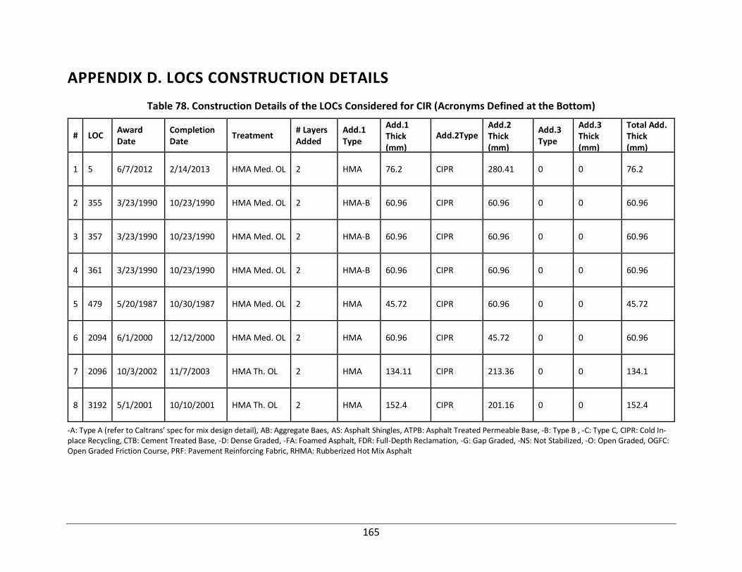
165

APPENDIX D. LOCS CONSTRUCTION DETAILS

Table 78. Construction Details of the LOCs Considered for CIR (Acronyms Defined at the Bottom)

# LOC Award Date

Completion Date

Treatment # Layers Added

Add.1 Type

Add.1 Thick (mm)

Add.2Type Add.2 Thick (mm)

Add.3 Type

Add.3 Thick (mm)

Total Add. Thick (mm)

1 5 6/7/2012 2/14/2013 HMA Med. OL 2 HMA 76.2 CIPR 280.41 0 0 76.2

2 355 3/23/1990 10/23/1990 HMA Med. OL 2 HMA-B 60.96 CIPR 60.96 0 0 60.96





7 2096 10/3/2002 11/7/2003 HMA Th. OL 2 HMA 134.11 CIPR 213.36 0 0 134.1

8 3192 5/1/2001 10/10/2001 HMA Th. OL 2 HMA 152.4 CIPR 201.16 0 0 152.4

-A: Type A (refer to Caltrans’ spec for mix design detail), AB: Aggregate Baes, AS: Asphalt Shingles, ATPB: Asphalt Treated Permeable Base, -B: Type B , -C: Type C, CIPR: Cold In-place Recycling, CTB: Cement Treated Base, -D: Dense Graded, -FA: Foamed Asphalt, FDR: Full-Depth Reclamation, -G: Gap Graded, -NS: Not Stabilized, -O: Open Graded, OGFC: Open Graded Friction Course, PRF: Pavement Reinforcing Fabric, RHMA: Rubberized Hot Mix Asphalt

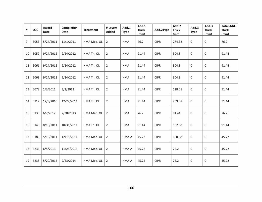
166

# LOC Award Date

Completion Date


Add.1 Type

Add.1 Thick (mm)


Add.3 Type

Add.3 Thick (mm)



10 5059 9/24/2012 9/24/2012 HMA Th. OL 2 HMA 91.44 CIPR 304.8 0 0 91.44

11 5061 9/24/2012 9/24/2012 HMA Th. OL 2 HMA 91.44 CIPR 304.8 0 0 91.44

12 5063 9/24/2012 9/24/2012 HMA Th. OL 2 HMA 91.44 CIPR 304.8 0 0 91.44

13 5078 1/3/2011 3/2/2012 HMA Th. OL 2 HMA 91.44 CIPR 128.01 0 0 91.44

14 5117 12/8/2010 12/22/2011 HMA Th. OL 2 HMA 91.44 CIPR 259.08 0 0 91.44


16 5143 8/10/2011 10/31/2011 HMA Th. OL 2 HMA 91.44 CIPR 182.88 0 0 91.44

17 5189 5/10/2011 12/15/2011 HMA Med. OL 2 HMA-A 45.72 CIPR 100.58 0 0 45.72



167

# LOC Award Date

Completion Date


Add.1 Type

Add.1 Thick (mm)


Add.3 Type

Add.3 Thick (mm)













168

# LOC Award Date

Completion Date


Add.1 Type

Add.1 Thick (mm)


Add.3 Type

Add.3 Thick (mm)



32 6525 6/27/2007 11/15/2007 CIPR 2 HMA 30.48 CIPR 48.77 0 0 30.48






38 7337 6/24/2002 2/28/2003 CIPR 2 ChipSealAR 0 CIPR 152.4 0 0 0


40 10091 5/8/2014 7/21/2015 CIPR 2 RHMA-G 30.48 CIPR 100.58 0 0 30.48

41 10093 5/8/2014 7/21/2015 CIPR 2 RHMA-G 30.48 CIPR 100.58 0 0 30.48

169

# LOC Award Date

Completion Date


Add.1 Type

Add.1 Thick (mm)


Add.3 Type

Add.3 Thick (mm)


42 11696 4/8/2011 11/29/2011 CIPR 2 HMA-A 30.48 CIPR 76.2 0 0 30.48

43 11767 4/29/2013 9/11/2013 HMA Med. OL 3 HMA-A 45.72 ChipSeal 0 CIPR 100.58 45.72





48 12582 5/23/2008 10/2/2008 HMA Med. OL 2 RHMA-G 39.62 CIPR 64.01 0 0 39.62




52 12983 5/21/2013 2/14/2014 HMA Med. OL 2 HMA-C 45.72 CIPR 91.44 0 0 45.72

170

# LOC Award Date

Completion Date


Add.1 Type

Add.1 Thick (mm)


Add.3 Type

Add.3 Thick (mm)





56 13759 3/23/1983 6/23/1983 CIPR 2 HMA 18.29 CIPR 18.29 0 0 18.29

57 14598 2/20/1990 5/11/1990 CIPR 2 HMA 30.48 CIPR 91.44 0 0 30.48

58 14832 6/20/2012 6/28/2013 HMA Th. OL 2 HMA-A 91.44 CIPR 91.44 0 0 91.44

59 15093 5/9/2011 7/11/2012 HMA Th. OL 3 HMA-A 106.68 HMA-A 152.4 CIPR 106.68 259.1





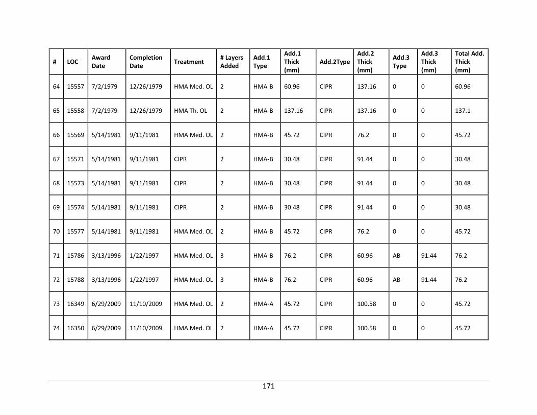
171

# LOC Award Date

Completion Date


Add.1 Type

Add.1 Thick (mm)


Add.3 Type

Add.3 Thick (mm)



65 15558 7/2/1979 12/26/1979 HMA Th. OL 2 HMA-B 137.16 CIPR 137.16 0 0 137.1


67 15571 5/14/1981 9/11/1981 CIPR 2 HMA-B 30.48 CIPR 91.44 0 0 30.48

68 15573 5/14/1981 9/11/1981 CIPR 2 HMA-B 30.48 CIPR 91.44 0 0 30.48

69 15574 5/14/1981 9/11/1981 CIPR 2 HMA-B 30.48 CIPR 91.44 0 0 30.48


71 15786 3/13/1996 1/22/1997 HMA Med. OL 3 HMA-B 76.2 CIPR 60.96 AB 91.44 76.2

72 15788 3/13/1996 1/22/1997 HMA Med. OL 3 HMA-B 76.2 CIPR 60.96 AB 91.44 76.2



172

# LOC Award Date

Completion Date


Add.1 Type

Add.1 Thick (mm)


Add.3 Type

Add.3 Thick (mm)



76 16453 5/5/2011 1/24/2012 CIPR 2 HMA-A 30.48 CIPR 100.58 0 0 30.48

77 16455 5/5/2011 1/24/2012 CIPR 2 HMA-A 30.48 CIPR 100.58 0 0 30.48




81 16549 8/26/1993 8/19/1994 CIPR 2 RHMA-G 30.48 CIPR 45.72 0 0 30.48

82 16551 8/26/1993 8/19/1994 CIPR 2 RHMA-G 30.48 CIPR 45.72 0 0 30.48

83 16553 8/26/1993 8/19/1994 CIPR 2 RHMA-G 30.48 CIPR 45.72 0 0 30.48

84 16555 8/26/1993 8/19/1994 CIPR 2 RHMA-G 30.48 CIPR 45.72 0 0 30.48

85 16559 8/26/1993 8/19/1994 CIPR 2 RHMA-G 30.48 CIPR 45.72 0 0 30.48

173

# LOC Award Date

Completion Date


Add.1 Type

Add.1 Thick (mm)


Add.3 Type

Add.3 Thick (mm)


86 16561 8/26/1993 8/19/1994 CIPR 2 RHMA-G 30.48 CIPR 45.72 0 0 30.48

87 16567 8/26/1993 8/19/1994 CIPR 2 RHMA-G 30.48 CIPR 45.72 0 0 30.48








95 18115 4/14/2009 10/19/2009 CIPR 2 HMA-A 30.48 CIPR 100.58 0 0 30.48

96 18248 5/4/2012 8/30/2012 CIPR 2 HMA-A 30.48 CIPR 100.58 0 0 30.48

174

# LOC Award Date

Completion Date


Add.1 Type

Add.1 Thick (mm)


Add.3 Type

Add.3 Thick (mm)


97 18249 5/6/2011 8/26/2011 CIPR 2 HMA-A 30.48 CIPR 100.58 0 0 30.48

98 18321 3/1/2012 12/10/2012 CIPR 2 HMA-A 30.48 CIPR 100.58 0 0 30.48

99 18325 3/6/2012 7/31/2012 CIPR 2 HMA-A 30.48 CIPR 106.68 0 0 30.48


101 18391 5/2/2013 10/23/2013 CIPR 2 HMA-A 30.48 CIPR 100.58 0 0 30.48

102 18422 5/6/2013 9/4/2013 CIPR 2 HMA-A 30.48 CIPR 100.58 0 0 30.48





107 18637 6/9/2014 5/16/2015 HMA Med. OL 2 RHMA-G 45.72 CIPR 76.2 0 0 45.72

175

# LOC Award Date

Completion Date


Add.1 Type

Add.1 Thick (mm)


Add.3 Type

Add.3 Thick (mm)

Total Add. Thick (mm) 108 18660 5/15/2015 10/15/2015 HMA Med. OL 2 HMA-A 45.72 CIPR 100.58 0 0 45.72




112 18746 12/3/2014 10/15/2015 CIPR 2 RHMA-G 30.48 CIPR 106.68 0 0 30.48









176

Table 79. Construction Details of the LOCs Considered for FDR

LOC Award Date

Completion Date


Add.1 Type

Add.1 Thick (mm)

Add.2 Type

Add.2 Thick (mm)

Add.3 Type

Add.3 Thick (mm)

Add.4 Type

Add.4 Thick (mm)

Add.5 Type

Add.5 Thick (mm)


1 8/31/11 8/31/11 FDR 2 HMA-A 137.16 FDR-NS 167.64 0 0.00 0 0.00 0 0.00 137.16

9 12/12/80 12/12/80 FDR 3 HMA 106.68 FDR-NS 137.16 AS 335.28 0 0.00 0 0.00 106.68

15 1/27/78 1/27/78 FDR 2 HMA-B 91.44 FDR-NS 152.40 0 0.00 0 0.00 0 0.00 91.44

17 1/27/78 1/27/78 FDR 2 HMA-B 91.44 FDR-NS 91.44 0 0.00 0 0.00 0 0.00 91.44

63 11/26/74 11/26/74 FDR 3 HMA 106.68 FDR-NS 137.16 AS 289.56 0 0.00 0 0.00 106.68

64 11/26/74 11/26/74 FDR 3 HMA 106.68 FDR-NS 137.16 AS 289.56 0 0.00 0 0.00 106.68

67 3/8/82 3/8/82 FDR 3 HMA 121.92 FDR-NS 152.40 AS 350.52 0 0.00 0 0.00 121.92

69 10/4/77 10/4/77 FDR 3 HMA 106.68 FDR-NS 167.64 AS 259.08 0 0.00 0 0.00 106.68

73 11/1/77 11/1/77 FDR 2 HMA 91.44 FDR-NS 106.68 0 0.00 0 0.00 0 0.00 91.44

75 12/20/76 12/20/76 FDR 2 HMA 91.44 FDR-NS 106.68 0 0.00 0 0.00 0 0.00 91.44

85 11/10/77 11/10/77 FDR 3 HMA-B 121.92 FDR-NS 137.16 AS.C4 320.04 0 0.00 0 0.00 121.92

89 4/1/74 4/1/74 FDR 2 HMA 121.92 FDR-NS 167.64 0 0.00 0 0.00 0 0.00 121.92

91 7/20/77 7/20/77 FDR 2 HMA 137.16 FDR-NS 274.32 0 0.00 0 0.00 0 0.00 137.16

97 2/21/78 2/21/78 FDR 3 HMA 121.92 FDR-NS 182.88 AS 213.36 0 0.00 0 0.00 121.92


111 5/11/77 5/11/77 FDR 2 HMA-B 121.92 FDR-NS 137.16 0 0.00 0 0.00 0 0.00 121.92


153 4/9/79 4/9/79 FDR 2 HMA-B 54.86 FDR-NS 274.32 0 0.00 0 0.00 0 0.00 54.86


175 8/29/83 8/29/83 FDR 2 HMA-B 137.16 FDR-NS 152.40 0 0.00 0 0.00 0 0.00 137.16




221 1/22/03 1/22/03 FDR 3 OGFC 24.38 HMA-B 152.40 FDR-NS 457.20 0 0.00 0 0.00 176.78

177

LOC Award Date

Completion Date


Add.1 Type

Add.1 Thick (mm)

Add.2 Type

Add.2 Thick (mm)

Add.3 Type

Add.3 Thick (mm)

Add.4 Type

Add.4 Thick (mm)

Add.5 Type

Add.5 Thick (mm)


234 1/1/93 1/1/93 FDR 3 HMA-B 137.16 ATPB 76.20 FDR-NS 387.10 0 0.00 0 0.00 213.36


292 3/6/00 3/6/00 FDR 4 HMA-B 167.64 ATPB 76.20 FDR-NS 152.40 AS.C2 350.52 0 0.00 243.84


410 3/14/83 3/14/83 FDR 2 HMA-B 152.40 FDR-NS 274.32 0 0.00 0 0.00 0 0.00 152.40

699 2/26/90 2/26/90 FDR 2 HMA-B 60.96 FDR-NS 152.40 0 0.00 0 0.00 0 0.00 60.96

708 1/4/99 1/4/99 FDR 4 OGFC 45.72 HMA-B 137.16 ATPB 76.20 FDR-NS 426.72 0 0.00 259.08

762 3/11/91 3/11/91 FDR 2 HMA-B 121.92 FDR-NS 350.52 0 0.00 0 0.00 0 0.00 121.92

789 3/8/99 3/8/99 FDR 2 HMA-B 91.44 FDR-NS 170.69 0 0.00 0 0.00 0 0.00 91.44

794 2/24/92 2/24/92 FDR 2 HMA-B 121.92 FDR-NS 396.24 0 0.00 0 0.00 0 0.00 121.92

847 3/27/95 3/27/95 FDR 2 HMA-B 137.16 FDR-NS 487.68 0 0.00 0 0.00 0 0.00 137.16

1015 1/1/97 1/1/97 FDR 2 HMA-B 152.40 FDR-NS 365.76 0 0.00 0 0.00 0 0.00 152.40

1201 12/1/98 12/1/98 FDR 2 HMA-B 76.20 FDR-NS 320.04 0 0.00 0 0.00 0 0.00 76.20

1285 12/23/08 12/23/08 FDR 3 OGFC 48.77 HMA-A 118.87 FDR-NS 173.74 0 0.00 0 0.00 167.64

1466 2/23/11 2/23/11 FDR 3 HMA-A 91.44 FDR-NS 259.08 FDR-NS 152.40 0 0.00 0 0.00 91.44

1604 6/6/92 6/6/92 FDR 2 HMA-A 137.16 FDR-NS 243.84 0 0.00 0 0.00 0 0.00 137.16

1755 6/30/95 6/30/95 FDR 4 RHMA-G 45.72 SAMI-R 0.00 HMA-A 115.82 FDR-NS 320.04 0 0.00 161.54

1810 6/11/90 6/11/90 FDR 3 HMA-A 60.96 ATPB 76.20 FDR-NS 320.04 0 0.00 0 0.00 137.16


1863 6/30/89 6/30/89 FDR 2 HMA-B 121.92 FDR-NS 106.68 0 0.00 0 0.00 0 0.00 121.92

2005 6/17/91 6/17/91 FDR 2 HMA-A 121.92 FDR-NS 304.80 0 0.00 0 0.00 0 0.00 121.92

2011 11/27/96 11/27/96 FDR 2 HMA-A 91.44 FDR-NS 472.44 0 0.00 0 0.00 0 0.00 91.44

2048 5/23/93 5/23/93 FDR 2 HMA-A 152.40 FDR-NS 259.08 0 0.00 0 0.00 0 0.00 152.40

2060 3/21/92 3/21/92 FDR 3 HMA-A 60.96 HMA-A 76.20 FDR-NS 259.08 0 0.00 0 0.00 137.16

2064 7/18/99 7/18/99 FDR 2 HMA-A 118.87 FDR-NS 210.31 0 0.00 0 0.00 0 0.00 118.87

2071 6/24/93 6/24/93 FDR 3 HMA-B 121.92 FDR-NS 381.00 FDR-NS 121.92 0 0.00 0 0.00 121.92

178

LOC Award Date

Completion Date


Add.1 Type

Add.1 Thick (mm)

Add.2 Type

Add.2 Thick (mm)

Add.3 Type

Add.3 Thick (mm)

Add.4 Type

Add.4 Thick (mm)

Add.5 Type

Add.5 Thick (mm)


2092 4/20/92 4/20/92 FDR 2 HMA-A 152.40 FDR-NS 106.68 0 0.00 0 0.00 0 0.00 152.40

2192 12/24/90 12/24/90 FDR 2 HMA-A 91.44 FDR-NS 335.28 0 0.00 0 0.00 0 0.00 91.44

2194 7/17/91 7/17/91 FDR 2 HMA-A 91.44 FDR-NS 335.28 0 0.00 0 0.00 0 0.00 91.44

2195 7/17/91 7/17/91 FDR 2 HMA-A 91.44 FDR-NS 335.28 0 0.00 0 0.00 0 0.00 91.44

2198 7/19/93 7/19/93 FDR 2 HMA-A 91.44 FDR-NS 259.08 0 0.00 0 0.00 0 0.00 91.44

2200 1/1/94 1/1/94 FDR 3 HMA-A 91.44 FDR-NS 259.08 SEG 0.00 0 0.00 0 0.00 91.44


2264 12/10/90 12/10/90 FDR 2 HMA-B 121.92 FDR-NS 106.68 0 0.00 0 0.00 0 0.00 121.92

2266 12/10/90 12/10/90 FDR 2 HMA-B 121.92 FDR-NS 335.28 0 0.00 0 0.00 0 0.00 121.92

2283 6/10/91 6/10/91 FDR 4 HMA-A 60.96 GPI 0.00 HMA-A 60.96 FDR-NS 320.04 0 0.00 121.92

2285 10/8/96 10/8/96 FDR 2 HMA-A 237.74 FDR-NS 137.16 0 0.00 0 0.00 0 0.00 237.74

2287 7/20/98 7/20/98 FDR 2 HMA-A 149.35 FDR-NS 359.66 0 0.00 0 0.00 0 0.00 149.35

2289 3/12/90 3/12/90 FDR 2 HMA-A 137.16 FDR-NS 106.68 0 0.00 0 0.00 0 0.00 137.16


2369 1/1/98 1/1/98 FDR 2 HMA-A 149.35 FDR-NS 274.32 0 0.00 0 0.00 0 0.00 149.35

2416 1/31/94 1/31/94 FDR 2 HMA-A 152.40 FDR-NS 365.76 0 0.00 0 0.00 0 0.00 152.40

2477 1/1/96 1/1/96 FDR 2 HMA-A 121.92 FDR-NS 106.68 0 0.00 0 0.00 0 0.00 121.92

2479 1/1/93 1/1/93 FDR 2 HMA-A 137.16 FDR-NS 106.68 0 0.00 0 0.00 0 0.00 137.16

2583 1/1/94 1/1/94 FDR 2 HMA-A 167.64 FDR-NS 243.84 0 0.00 0 0.00 0 0.00 167.64


2738 8/6/98 8/6/98 FDR 2 HMA-A 118.87 FDR-NS 103.63 0 0.00 0 0.00 0 0.00 118.87

2857 12/20/03 12/20/03 FDR 2 HMA 179.83 FDR-NS 374.90 0 0.00 0 0.00 0 0.00 179.83


2883 11/19/04 11/19/04 FDR 2 HMA-A 134.11 FDR-NS 103.63 0 0.00 0 0.00 0 0.00 134.11


2970 11/5/02 11/5/02 FDR 2 HMA-A 118.87 FDR-NS 271.27 0 0.00 0 0.00 0 0.00 118.87

179

LOC Award Date

Completion Date


Add.1 Type

Add.1 Thick (mm)

Add.2 Type

Add.2 Thick (mm)

Add.3 Type

Add.3 Thick (mm)

Add.4 Type

Add.4 Thick (mm)

Add.5 Type

Add.5 Thick (mm)


3065 11/11/03 11/11/03 FDR 3 HMA-A 134.11 GPI 0.00 FDR-NS 103.63 0 0.00 0 0.00 134.11

3106 9/22/00 9/22/00 FDR 2 HMA-A 149.35 FDR-NS 271.27 0 0.00 0 0.00 0 0.00 149.35

3198 10/20/04 10/20/04 FDR 2 HMA-A 149.35 FDR-NS 344.42 0 0.00 0 0.00 0 0.00 149.35

3229 10/27/06 10/27/06 FDR 2 HMA-A 134.11 FDR-NS 103.63 0 0.00 0 0.00 0 0.00 134.11

3319 11/17/11 11/17/11 FDR 2 HMA-A 182.88 FDR-NS 463.30 0 0.00 0 0.00 0 0.00 182.88

3321 11/17/11 11/17/11 FDR 3 RHMA-O 30.48 HMA 182.88 FDR-NS 457.20 0 0.00 0 0.00 213.36


3333 1/1/01 1/1/01 FDR 2 HMA-A 149.35 FDR-NS 256.03 0 0.00 0 0.00 0 0.00 149.35

3342 11/13/08 11/13/08 FDR 3 RHMA-D 45.72 HMA-A 85.34 FDR-NS 313.94 0 0.00 0 0.00 131.06

3402 9/4/07 9/4/07 FDR 3 HMA 149.35 FDR-NS 329.18 SEG 0.00 0 0.00 0 0.00 149.35


3406 1/17/06 1/17/06 FDR 2 HMA-A 152.40 FDR-NS 243.84 0 0.00 0 0.00 0 0.00 152.40

3445 8/31/06 8/31/06 FDR 2 HMA-A 149.35 FDR-NS 320.04 0 0.00 0 0.00 0 0.00 149.35

3459 10/12/09 10/12/09 FDR 2 HMA-A 167.64 FDR-NS 106.68 0 0.00 0 0.00 0 0.00 167.64

3862 5/4/01 1/12/02 FDR 3 OGFC 21.34 HMA 45.72 FDR-FA 228.60 0 0.00 0 0.00 67.06

3866 5/4/01 1/12/02 FDR 3 OGFC 21.34 HMA 45.72 FDR-FA 228.60 0 0.00 0 0.00 67.06

3999 4/27/01 5/31/02 FDR 3 OGFC 18.29 HMA 164.59 FDR-NS 478.54 0 0.00 0 0.00 182.88

4821 3/10/06 4/21/09 FDR 5 OGFC 30.48 HMA-A 45.72 HMA-A 152.40 FDR-NS 182.88 LTS 304.80 228.60





5121 11/15/13 11/15/13 FDR 2 HMA-A 152.40 FDR-NS 182.88 0 0.00 0 0.00 0 0.00 152.40


5171 5/20/11 5/20/11 FDR 3 HMA 152.40 FDR-NS 60.96 AS 30.48 0 0.00 0 0.00 152.40


180

LOC Award Date

Completion Date


Add.1 Type

Add.1 Thick (mm)

Add.2 Type

Add.2 Thick (mm)

Add.3 Type

Add.3 Thick (mm)

Add.4 Type

Add.4 Thick (mm)

Add.5 Type

Add.5 Thick (mm)


5378 9/28/09 9/28/09 FDR 2 HMA-A 152.40 FDR-NS 167.64 0 0.00 0 0.00 0 0.00 152.40

5379 10/19/06 10/19/06 FDR 2 HMA-A 149.35 FDR-NS 286.51 0 0.00 0 0.00 0 0.00 149.35

5380 10/19/06 10/19/06 FDR 2 HMA-A 149.35 FDR-NS 286.51 0 0.00 0 0.00 0 0.00 149.35

5381 8/17/07 8/17/07 FDR 2 HMA-A 149.35 FDR-NS 256.03 0 0.00 0 0.00 0 0.00 149.35

5383 10/10/08 10/10/08 FDR 2 HMA-A 149.35 FDR-NS 289.56 0 0.00 0 0.00 0 0.00 149.35

5500 1/1/05 1/1/05 FDR 2 HMA 155.45 FDR-NS 353.57 0 0.00 0 0.00 0 0.00 155.45

5506 9/28/07 9/28/07 FDR 2 HMA-A 137.16 FDR-NS 304.80 0 0.00 0 0.00 0 0.00 137.16

5508 11/28/07 11/28/07 FDR 2 HMA-A 118.87 FDR-NS 313.94 0 0.00 0 0.00 0 0.00 118.87

5514 11/11/10 3/8/12 FDR 2 HMA 121.92 FDR-FA 304.80 0 0.00 0 0.00 0 0.00 121.92

5530 10/14/09 10/14/09 FDR 2 HMA-A 167.64 FDR-NS 198.12 0 0.00 0 0.00 0 0.00 167.64


5540 2/13/12 3/6/13 FDR 4 HMA-A 152.40 FDR-FA 381.00 GPI 0.00 AS.C4 609.60 0 0.00 152.40

5544 12/5/07 12/5/07 FDR 2 HMA-A 121.92 FDR-NS 304.80 0 0.00 0 0.00 0 0.00 121.92

5548 10/22/13 10/22/13 FDR 2 HMA-A 137.16 FDR-NS 396.24 0 0.00 0 0.00 0 0.00 137.16

5590 12/10/07 12/10/07 FDR 2 HMA-A 164.59 FDR-NS 374.90 0 0.00 0 0.00 0 0.00 164.59

5632 10/8/13 10/8/13 FDR 2 HMA-A 121.92 FDR-NS 152.40 0 0.00 0 0.00 0 0.00 121.92

5652 12/14/11 10/25/13 FDR 3 RHMA-O 30.48 HMA 213.36 FDR-NS 563.88 0 0.00 0 0.00 243.84

5729 5/17/13 10/28/13 FDR 2 HMA-A 121.92 FDR-NS 182.88 0 0.00 0 0.00 0 0.00 121.92

5765 3/18/14 6/26/14 FDR 2 HMA-A 106.68 FDR-NS 228.60 0 0.00 0 0.00 0 0.00 106.68

5822 5/14/02 8/22/02 FDR 2 HMA-A 45.72 FDR-FA 204.22 0 0.00 0 0.00 0 0.00 45.72

6083 2/18/03 10/31/05 FDR 4 OGFC 24.38 FDR-FA 195.07 FDR-NS 286.51 AS.C2 225.55 0 0.00 24.38




6122 2/9/06 7/27/06 FDR 2 HMA-A 48.77 FDR-FA 225.55 0 0.00 0 0.00 0 0.00 48.77

6135 11/22/06 12/13/07 FDR 3 RHMA-O 30.48 HMA-A 198.12 FDR-NS 579.12 0 0.00 0 0.00 228.60

181

LOC Award Date

Completion Date


Add.1 Type

Add.1 Thick (mm)

Add.2 Type

Add.2 Thick (mm)

Add.3 Type

Add.3 Thick (mm)

Add.4 Type

Add.4 Thick (mm)

Add.5 Type

Add.5 Thick (mm)


6137 11/22/06 12/13/07 FDR 3 RHMA-O 30.48 HMA-A 198.12 FDR-NS 579.12 0 0.00 0 0.00 228.60

7164 12/17/08 7/1/11 FDR 4 RHMA-G 45.72 HMA 167.64 FDR-NS 350.52 AS.C1 335.28 0 0.00 213.36



7594 10/20/10 10/20/10 FDR 2 HMA-A 91.44 FDR-FA 304.80 0 0.00 0 0.00 0 0.00 91.44

7707 6/3/15 10/14/15 FDR 2 HMA-A 91.44 FDR-NS 259.08 0 0.00 0 0.00 0 0.00 91.44

7801 11/3/05 11/3/05 FDR 4 HMA-A 225.55 ATPB 76.20 HMA-A 118.87 FDR-NS 762.00 0 0.00 420.62

7802 11/3/05 11/3/05 FDR 4 HMA-A 225.55 ATPB 76.20 FDR-NS 271.27 AS.C4 435.86 0 0.00 301.75


7908 5/11/09 5/11/09 FDR 3 RHMA-G 30.48 HMA-A 152.40 FDR-NS 554.74 0 0.00 0 0.00 182.88

7937 12/24/03 12/24/03 FDR 4 RHMA-O 30.48 HMA-A 134.11 FDR-NS 286.51 AS.C4 359.66 0 0.00 164.59



8010 4/30/12 4/30/12 FDR 5 RHMA-G 45.72 HMA-A 76.20 FDR-NS 195.07 PM 298.70 AS.C4 298.70 121.92

8024 10/15/97 10/15/97 FDR 3 HMA-A 137.16 FDR-NS 213.36 AS.C4 304.80 0 0.00 0 0.00 137.16

8057 7/17/06 7/17/06 FDR 3 HMA 182.88 FDR-NS 45.72 AS 457.20 0 0.00 0 0.00 182.88

8061 8/19/91 8/19/91 FDR 5 HMA-A 121.92 ATPB 76.20 CTB 152.40 FDR-NS 152.40 PM 304.80 350.52

8063 8/19/91 8/19/91 FDR 5 HMA-A 121.92 ATPB 76.20 CTB 152.40 FDR-NS 152.40 PM 304.80 350.52


8106 10/23/07 10/23/07 FDR 2 HMA-A 271.27 FDR-NS 271.27 0 0.00 0 0.00 0 0.00 271.27

8112 10/23/07 10/23/07 FDR 2 HMA-A 271.27 FDR-NS 271.27 0 0.00 0 0.00 0 0.00 271.27

8123 7/5/11 7/5/11 FDR 2 HMA-A 152.40 FDR-NS 152.40 0 0.00 0 0.00 0 0.00 152.40

8124 7/5/11 7/5/11 FDR 2 HMA-A 152.40 FDR-NS 152.40 0 0.00 0 0.00 0 0.00 152.40

8183 10/5/00 10/5/00 FDR 4 OGFC 30.48 HMA-A 152.40 FDR-NS 243.84 AS.C4 152.40 0 0.00 182.88

8205 8/8/95 8/8/95 FDR 2 HMA-A 60.96 FDR-NS 243.84 0 0.00 0 0.00 0 0.00 60.96


182

LOC Award Date

Completion Date


Add.1 Type

Add.1 Thick (mm)

Add.2 Type

Add.2 Thick (mm)

Add.3 Type

Add.3 Thick (mm)

Add.4 Type

Add.4 Thick (mm)

Add.5 Type

Add.5 Thick (mm)






8295 3/26/94 3/26/94 FDR 5 OGFC 30.48 HMA-A 198.12 ATPB 76.20 FDR-NS 182.88 AS.C4 274.32 304.80






8321 10/5/09 10/5/09 FDR 4 RHMA-G 45.72 HMA-A 100.58 FDR-NS 298.70 AS.C4 240.79 0 0.00 146.30


11302 10/7/02 12/18/03 FDR 2 HMA-A 76.20 FDR-FA 176.78 0 0.00 0 0.00 0 0.00 76.20

11321 9/10/04 9/10/04 FDR 2 HMA-B 243.84 FDR-NS 259.08 0 0.00 0 0.00 0 0.00 243.84

11338 3/15/05 3/15/05 FDR 2 HMA 152.40 FDR-NS 505.97 0 0.00 0 0.00 0 0.00 152.40

11340 3/17/05 3/17/05 FDR 2 HMA-B 152.40 FDR-NS 396.24 0 0.00 0 0.00 0 0.00 152.40

11380 10/14/04 4/7/06 FDR 2 HMA-B 76.20 FDR-FA 201.17 0 0.00 0 0.00 0 0.00 76.20

11384 10/14/04 4/7/06 FDR 2 HMA-B 76.20 FDR-FA 201.17 0 0.00 0 0.00 0 0.00 76.20

11421 12/12/06 12/12/06 FDR 2 HMA-B 152.40 FDR-NS 201.17 0 0.00 0 0.00 0 0.00 152.40

11423 12/12/06 12/12/06 FDR 2 HMA-B 152.40 FDR-NS 201.17 0 0.00 0 0.00 0 0.00 152.40

11452 8/24/07 8/24/07 FDR 3 HMA 152.40 ATPB 76.20 FDR-NS 310.90 0 0.00 0 0.00 228.60



11545 9/24/09 9/24/09 FDR 2 HMA 152.40 FDR-NS 335.28 0 0.00 0 0.00 0 0.00 152.40

11547 9/25/09 9/25/09 FDR 2 HMA-B 121.92 FDR-NS 201.17 0 0.00 0 0.00 0 0.00 121.92

11573 2/1/10 2/1/10 FDR 3 RHMA-G 24.38 HMA-B 228.60 FDR-NS 883.92 0 0.00 0 0.00 252.98

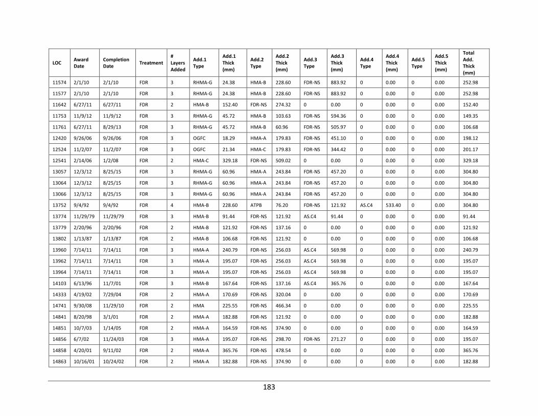
183

LOC Award Date

Completion Date


Add.1 Type

Add.1 Thick (mm)

Add.2 Type

Add.2 Thick (mm)

Add.3 Type

Add.3 Thick (mm)

Add.4 Type

Add.4 Thick (mm)

Add.5 Type

Add.5 Thick (mm)




11642 6/27/11 6/27/11 FDR 2 HMA-B 152.40 FDR-NS 274.32 0 0.00 0 0.00 0 0.00 152.40




12524 11/2/07 11/2/07 FDR 3 OGFC 21.34 HMA-C 179.83 FDR-NS 344.42 0 0.00 0 0.00 201.17

12541 2/14/06 1/2/08 FDR 2 HMA-C 329.18 FDR-NS 509.02 0 0.00 0 0.00 0 0.00 329.18






13779 2/20/96 2/20/96 FDR 2 HMA-B 121.92 FDR-NS 137.16 0 0.00 0 0.00 0 0.00 121.92

13802 1/13/87 1/13/87 FDR 2 HMA-B 106.68 FDR-NS 121.92 0 0.00 0 0.00 0 0.00 106.68





14333 4/19/02 7/29/04 FDR 2 HMA-A 170.69 FDR-NS 320.04 0 0.00 0 0.00 0 0.00 170.69

14741 9/30/08 11/29/10 FDR 2 HMA 225.55 FDR-NS 466.34 0 0.00 0 0.00 0 0.00 225.55

14841 8/20/98 3/1/01 FDR 2 HMA-A 182.88 FDR-NS 121.92 0 0.00 0 0.00 0 0.00 182.88

14851 10/7/03 1/14/05 FDR 2 HMA-A 164.59 FDR-NS 374.90 0 0.00 0 0.00 0 0.00 164.59


14858 4/20/01 9/11/02 FDR 2 HMA-A 365.76 FDR-NS 478.54 0 0.00 0 0.00 0 0.00 365.76

14863 10/16/01 10/24/02 FDR 2 HMA-A 182.88 FDR-NS 374.90 0 0.00 0 0.00 0 0.00 182.88

184

LOC Award Date

Completion Date


Add.1 Type

Add.1 Thick (mm)

Add.2 Type

Add.2 Thick (mm)

Add.3 Type

Add.3 Thick (mm)

Add.4 Type

Add.4 Thick (mm)

Add.5 Type

Add.5 Thick (mm)


14866 10/16/01 10/24/02 FDR 2 HMA-A 182.88 FDR-NS 374.90 0 0.00 0 0.00 0 0.00 182.88

14875 11/17/00 9/13/01 FDR 2 HMA-A 225.55 FDR-NS 329.18 0 0.00 0 0.00 0 0.00 225.55

14903 10/4/00 11/28/01 FDR 2 HMA-A 195.07 FDR-NS 201.17 0 0.00 0 0.00 0 0.00 195.07

15015 9/24/04 9/24/04 FDR 2 HMA-A 179.83 FDR-NS 121.92 0 0.00 0 0.00 0 0.00 179.83

15069 12/18/07 12/18/07 FDR 2 HMA-A 195.07 FDR-NS 286.51 0 0.00 0 0.00 0 0.00 195.07

15070 12/18/07 12/18/07 FDR 2 HMA-A 195.07 FDR-NS 286.51 0 0.00 0 0.00 0 0.00 195.07

15071 12/18/07 12/18/07 FDR 2 HMA-A 195.07 FDR-NS 286.51 0 0.00 0 0.00 0 0.00 195.07

15072 12/18/07 12/18/07 FDR 2 HMA-A 195.07 FDR-NS 286.51 0 0.00 0 0.00 0 0.00 195.07

15099 4/6/12 1/9/14 FDR 2 HMA-A 198.12 FDR-NS 350.52 0 0.00 0 0.00 0 0.00 198.12

15102 6/8/09 9/20/10 FDR 2 HMA-A 179.83 FDR-NS 164.59 0 0.00 0 0.00 0 0.00 179.83

15104 6/8/09 9/20/10 FDR 2 HMA-A 179.83 FDR-NS 164.59 0 0.00 0 0.00 0 0.00 179.83


15198 9/27/07 9/27/07 FDR 2 HMA-A 213.36 FDR-NS 152.40 0 0.00 0 0.00 0 0.00 213.36

15201 5/30/07 4/2/08 FDR 2 HMA-A 137.16 FDR-NS 283.46 0 0.00 0 0.00 0 0.00 137.16

15248 2/3/12 2/3/12 FDR 2 HMA 213.36 FDR-NS 274.32 0 0.00 0 0.00 0 0.00 213.36

15878 10/30/08 6/3/10 FDR 2 HMA-A 155.45 FDR-NS 170.69 0 0.00 0 0.00 0 0.00 155.45



16279 9/10/08 7/24/09 FDR 2 RHMA-G 45.72 FDR-NS 103.63 0 0.00 0 0.00 0 0.00 45.72

16375 2/9/11 9/22/11 FDR 2 HMA-A 60.96 FDR-FA 167.64 0 0.00 0 0.00 0 0.00 60.96



16677 6/2/95 6/2/95 FDR 2 HMA-B 121.92 FDR-NS 259.08 0 0.00 0 0.00 0 0.00 121.92

16679 6/6/97 6/6/97 FDR 2 HMA-B 167.64 FDR-NS 15.24 0 0.00 0 0.00 0 0.00 167.64


185

LOC Award Date

Completion Date


Add.1 Type

Add.1 Thick (mm)

Add.2 Type

Add.2 Thick (mm)

Add.3 Type

Add.3 Thick (mm)

Add.4 Type

Add.4 Thick (mm)

Add.5 Type

Add.5 Thick (mm)


17158 3/30/11 3/30/11 FDR 5 OGFC 24.38 RHMA-G

60.96 HMA-A 121.92 FDR-NS 243.84 AS.C2 152.40 207.26

17179 8/29/06 2/22/08 FDR 3 HMA 350.52 FDR-NS 228.60 GPI 0.00 0 0.00 0 0.00 350.52

17181 8/29/06 2/22/08 FDR 3 HMA-A 91.44 FDR-NS 207.26 GPI 0.00 0 0.00 0 0.00 91.44




17206 2/23/05 8/30/06 FDR 3 RHMA-O 24.38 RHMA-G

60.96 FDR-FA 225.55 0 0.00 0 0.00 85.34

17208 2/23/05 8/30/06 FDR 3 RHMA-O 24.38 RHMA-G

60.96 FDR-FA 225.55 0 0.00 0 0.00 85.34

17214 11/20/07 4/22/09 FDR 2 HMA-A 103.63 FDR-FA 280.42 0 0.00 0 0.00 0 0.00 103.63

17216 11/20/07 4/22/09 FDR 2 HMA-A 134.11 FDR-FA 304.80 0 0.00 0 0.00 0 0.00 134.11

17218 11/20/07 4/22/09 FDR 2 HMA-A 134.11 FDR-FA 304.80 0 0.00 0 0.00 0 0.00 134.11

18456 7/8/03 9/20/04 FDR 2 HMA-A 210.31 FDR-NS 225.55 0 0.00 0 0.00 0 0.00 210.31

18460 7/8/03 9/20/04 FDR 2 HMA-A 210.31 FDR-NS 509.02 0 0.00 0 0.00 0 0.00 210.31

18465 7/20/99 1/9/01 FDR 2 HMA-A 167.64 FDR-NS 106.68 0 0.00 0 0.00 0 0.00 167.64

18469 7/20/99 1/9/01 FDR 2 HMA-A 167.64 FDR-NS 106.68 0 0.00 0 0.00 0 0.00 167.64

18472 7/20/99 1/9/01 FDR 2 HMA-A 167.64 FDR-NS 106.68 0 0.00 0 0.00 0 0.00 167.64

18480 7/20/99 1/9/01 FDR 2 HMA-A 182.88 FDR-NS 256.03 0 0.00 0 0.00 0 0.00 182.88

18492 10/4/06 6/4/09 FDR 2 HMA-A 179.83 FDR-NS 524.26 0 0.00 0 0.00 0 0.00 179.83

18493 10/4/06 6/4/09 FDR 2 HMA-A 179.83 FDR-NS 524.26 0 0.00 0 0.00 0 0.00 179.83

18494 10/4/06 6/4/09 FDR 2 HMA-A 179.83 FDR-NS 524.26 0 0.00 0 0.00 0 0.00 179.83

18499 10/4/06 6/4/09 FDR 2 HMA-A 179.83 FDR-NS 524.26 0 0.00 0 0.00 0 0.00 179.83

18501 10/4/06 6/4/09 FDR 2 HMA-A 179.83 FDR-NS 524.26 0 0.00 0 0.00 0 0.00 179.83

18700 1/4/11 10/30/15 FDR 2 HMA-A 243.84 FDR-NS 213.36 0 0.00 0 0.00 0 0.00 243.84

18702 1/4/11 10/30/15 FDR 2 HMA-A 243.84 FDR-NS 213.36 0 0.00 0 0.00 0 0.00 243.84

18705 1/4/11 10/30/15 FDR 2 HMA-A 243.84 FDR-NS 213.36 0 0.00 0 0.00 0 0.00 243.84

186

LOC Award Date

Completion Date


Add.1 Type

Add.1 Thick (mm)

Add.2 Type

Add.2 Thick (mm)

Add.3 Type

Add.3 Thick (mm)

Add.4 Type

Add.4 Thick (mm)

Add.5 Type

Add.5 Thick (mm)


18711 1/4/11 10/30/15 FDR 2 HMA-A 243.84 FDR-NS 213.36 0 0.00 0 0.00 0 0.00 243.84






18790 11/30/09 11/30/09 FDR 2 HMA-A 149.35 FDR-NS 554.74 0 0.00 0 0.00 0 0.00 149.35

18792 11/30/09 11/30/09 FDR 2 HMA-A 149.35 FDR-NS 554.74 0 0.00 0 0.00 0 0.00 149.35

18804 12/17/06 12/17/06 FDR 2 HMA-A 149.35 FDR-NS 149.35 0 0.00 0 0.00 0 0.00 149.35

18813 4/11/11 4/11/11 FDR 2 HMA-A 121.92 FDR-NS 411.48 0 0.00 0 0.00 0 0.00 121.92

18814 4/11/11 4/11/11 FDR 2 HMA-A 121.92 FDR-NS 411.48 0 0.00 0 0.00 0 0.00 121.92

18815 4/11/11 4/11/11 FDR 2 HMA-A 121.92 FDR-NS 411.48 0 0.00 0 0.00 0 0.00 121.92

18816 4/11/11 4/11/11 FDR 2 HMA-A 121.92 FDR-NS 411.48 0 0.00 0 0.00 0 0.00 121.92

18818 4/11/11 4/11/11 FDR 2 HMA-A 121.92 FDR-NS 182.88 0 0.00 0 0.00 0 0.00 121.92

18820 4/11/11 4/11/11 FDR 2 HMA-A 121.92 FDR-NS 182.88 0 0.00 0 0.00 0 0.00 121.92

18822 4/11/11 4/11/11 FDR 2 HMA-A 121.92 FDR-NS 411.48 0 0.00 0 0.00 0 0.00 121.92

18889 6/19/09 6/19/09 FDR 2 HMA-A 274.32 FDR-NS 103.63 0 0.00 0 0.00 0 0.00 274.32

18895 6/19/09 6/19/09 FDR 2 HMA-A 274.32 FDR-NS 103.63 0 0.00 0 0.00 0 0.00 274.32

18901 6/19/09 6/19/09 FDR 2 HMA-A 274.32 FDR-NS 103.63 0 0.00 0 0.00 0 0.00 274.32


18921 9/27/05 9/27/05 FDR 2 HMA-A 179.83 FDR-NS 673.61 0 0.00 0 0.00 0 0.00 179.83

18923 9/27/05 9/27/05 FDR 2 HMA-A 179.83 FDR-NS 673.61 0 0.00 0 0.00 0 0.00 179.83

18962 8/13/13 8/13/13 FDR 2 HMA-A 228.60 FDR-NS 45.72 0 0.00 0 0.00 0 0.00 228.60

18963 8/13/13 8/13/13 FDR 2 HMA-A 167.64 FDR-NS 106.68 0 0.00 0 0.00 0 0.00 167.64

18990 11/4/96 11/4/96 FDR 4 HMA-PM 182.88 ATPB 76.20 FDR-NS 228.60 AS.C2 304.80 0 0.00 259.08

18993 8/6/09 8/6/09 FDR 2 HMA-A 164.59 FDR-NS 103.63 0 0.00 0 0.00 0 0.00 164.59

187

LOC Award Date

Completion Date


Add.1 Type

Add.1 Thick (mm)

Add.2 Type

Add.2 Thick (mm)

Add.3 Type

Add.3 Thick (mm)

Add.4 Type

Add.4 Thick (mm)

Add.5 Type

Add.5 Thick (mm)


18997 8/6/09 8/6/09 FDR 4 RHMA-G 30.48 HMA-A 134.11 HMA-A 91.44 FDR-NS 103.63 0 0.00 256.03




19009 3/14/94 3/14/94 FDR 3 HMA-PM 137.16 ATPB 76.20 FDR-NS 91.44 0 0.00 0 0.00 213.36

19011 3/14/94 3/14/94 FDR 3 HMA-PM 137.16 ATPB 76.20 FDR-NS 121.92 0 0.00 0 0.00 213.36



19042 5/17/11 11/14/11 FDR 2 HMA-A 198.12 FDR-NS 243.84 0 0.00 0 0.00 0 0.00 198.12

19043 9/5/14 9/5/14 FDR 2 HMA-A 198.12 FDR-NS 335.28 0 0.00 0 0.00 0 0.00 198.12



19063 11/6/14 11/6/14 FDR 3 HMA-A 45.72 HMA-A 121.92 FDR-NS 137.16 0 0.00 0 0.00 167.64

19070 10/26/12 10/26/12 FDR 2 HMA-A 121.92 FDR-NS 365.76 0 0.00 0 0.00 0 0.00 121.92

19076 11/20/07 11/20/07 FDR 2 HMA-A 134.11 FDR-NS 368.81 0 0.00 0 0.00 0 0.00 134.11




19118 2/14/11 2/14/11 FDR 2 HMA-A 173.74 FDR-NS 329.18 0 0.00 0 0.00 0 0.00 173.74

19176 2/10/11 2/10/11 FDR 2 HMA-B 149.35 FDR-NS 274.32 0 0.00 0 0.00 0 0.00 149.35



19184 10/30/15 10/30/15 FDR 3 RHMA-D 45.72 HMA-A 103.63 FDR-NS 201.17 0 0.00 0 0.00 149.35




188

LOC Award Date

Completion Date


Add.1 Type

Add.1 Thick (mm)

Add.2 Type

Add.2 Thick (mm)

Add.3 Type

Add.3 Thick (mm)

Add.4 Type

Add.4 Thick (mm)

Add.5 Type

Add.5 Thick (mm)


19209 5/13/15 5/13/15 FDR 2 HMA-A 167.64 FDR-NS 441.96 0 0.00 0 0.00 0 0.00 167.64

19215 11/21/13 11/21/13 FDR 2 HMA-A 91.44 FDR-NS 152.40 0 0.00 0 0.00 0 0.00 91.44

-A: Type A (refer to Caltrans’ spec for mix design detail), AB: Aggregate Baes, AS: Asphalt Shingles, ATPB: Asphalt Treated Permeable Base, -B: Type B , -C: Type C, CIPR: Cold In-place Recycling, CTB: Cement Treated Base, -D: Dense Graded, -FA: Foamed Asphalt, FDR: Full-Depth Reclamation, -G: Gap Graded, -NS: Not Stabilized, -O: Open Graded, OGFC: Open Graded Friction Course, PRF: Pavement Reinforcing Fabric, RHMA: Rubberized Hot Mix Asphalt

189

APPENDIX E. HMA QUANTITY CALCULATION

Assuming that all the aggregate types (including RAP) selected in the design are put in a batch, the amount of aggregate type 𝑖 (𝑄𝑎𝑔𝑔,𝑖 , ) by the total weight of a batch (𝑄𝐵𝑎𝑡𝑐ℎ) should verify the

equation shown in Figure 153.

Figure 152. Equation. Mix design aggregate percent.

When RAP is used, the amount of recycled binder in the batch depends on the amount of recycled binder in aggregate type 𝑖 (𝑄𝑟𝑒𝑐𝑦𝑐𝑙𝑒𝑑 𝑏𝑖𝑛𝑑𝑒𝑟,𝑖) as shown in Figure 154; 𝛿𝑖,𝐵𝑎𝑡𝑐ℎ=0 when aggregate type 𝑖

is virgin aggregate. Therefore, the recycled binder in the batch is calculated as follows:

Figure 153. Equation. Batch recycled binder percent calculation.

The aggregate content 𝑄𝑎𝑔𝑔, 𝑛𝑜 𝑏𝑖𝑛𝑑𝑒𝑟 (does not include the weight of recycled binder in the batch) is

calculated using the formula shown in Figure 155.

Figure 154. Equation. Batch aggregate content calculation.

Since asphalt content (percent) of the AC mix (it includes the virgin binder and recycled binder contained in RAP) is known, the aggregate content in the AC mix is (Figure 156):

190

Figure 155. Equation. Aggregate content in AC calculation.

the percent of AC by the weight of batch should be (Figure 156):

Figure 156. Equation. AC percent in batch calculation.

And the amount of virgin binder by the weight of AC is calculated as follows (Figure 158):

Figure 157. Equation. Amount of virgin binder by weight of AC calculation.

The amount of aggregate type 𝑖 by the weight of AC is

Figure 158. Equation. Amount of aggregate type i by weight of AC calculation.

(1 g/cm3 = 0.8428 ton/yd3)

The bulk specific gravity Gsb (g/cm2) is used in AC quantity calculation and is expressed as follows (Figure 160):

191

Figure 159. Equation. Gsb calculation formula.

192

APPENDIX F: CASE STUDIES

Two case studies were conducted to compare the environmental impacts of in-place recycling techniques with conventional milling and overlay using the IPR tool. The wide range of treatment options and flexibility are significant advantages of using the IPR tool to conduct comparison LCA studies

CASE STUDY 1 COLD IN-PLACE RECYCLING AND FULL-DEPTH RECLAMATION

TREATMENT TYPES

The input data of the model are based on the study conducted by Saboori et al. (91) The functional unit of the case study is one lane-mile of pavement. Three types of recycling treatments were considered in this case study, cold in-place recycling (CIR) with chip seal, CIR with thin hot-mix asphalt (HMA) overlay, and full-depth reclamation (FDR) with medium overlay. For the FDR treatments, six mixture designs were considered for sensitivity analysis of the environmental impact from asphalt emulsion, fly ash, and cement. The cement content ranged from 0 percent to 6 percent with a substitution of 3 percent fly ash. Table 80 lists all treatments considered in the case study.

Table 80. Treatments Considered in the Study

Treatment Number

Type of Treatments

1 CIR (10 cm milled + Mech. Stab.) w. Chip Seal

2 CIR (10 cm milled + Mech. Stab.) w. 2.5 cm of HMA OL

3 FDR (25 cm milled + 4 percent AE + 1 percent PC) w. 6 cm RHMA OL

4 FDR (25 cm milled + 3 percent FA + 1 percent PC) w. 6 cm RHMA OL

5 FDR (25 cm milled + no stabilization) w. 6 cm RHMA OL

6 FDR (25 cm milled + 2 percent PC) w. 6 cm RHMA OL



9 Conventional Mill-and-fill treatment

* Mech. Stab.: mechanical stabilization; CIR: cold in-place recycling

FDR: full-depth reclamation; AE: asphalt emulsion; FA: foamed asphalt

OL: overlay; PC: Portland cement; RHMA: rubberized HMA (gap-graded)

Traffic Inputs

The traffic inputs are as follows: passenger car at 85 percent, small truck at 5 percent, medium truck at 5 percent, large truck at 5 percent, growth rate at 2 percent, and AADT at 4000. The assumptions for work zone are: speed limited at 60 mph, queue speed at 50 mph, work zone speed at 30 mph, and queue length for 1 mile. The inputs were assumed the same for various treatments, although the work zone schedule and traffic delay might have varied between various treatments.

193

Material Inputs

The material stage includes raw materials acquisition, plant production, and transportation from raw materials to job site. For transportation, a 50-mile distance was assumed which is an average distance in the State of California. Table 81 shows the material used per lane-mile in unit of U.S. ton.

Table 81. Material per Lane-Mile (Unit: U.S. ton)

Treatment Type Nature Agg.

Crushed Agg.

Asphalt Binder

HMA Operation

Asphalt Emulsion

Cement Fly Ash

Total

CIR (10 cm milled + Mech. Stab.) w. Chip Seal

- 123 - - 12 - - 135

CIR (10 cm milled + Mech. Stab.) w. 2.5 cm of HMA OL

43 141 11 197 11 - - 403

FDR (25 cm milled + 4 percent AE + 1 percent PC) w. 6 cm RHMA OL

103 338 26 473 46 11 - 998

FDR (25 cm milled + 3 percent FA + 1 percent PC) w. 6 cm RHMA OL

103 338 26 473 26 11 33 1011

FDR (25 cm milled + no stabilization) w. 6 cm RHMA OL

103 338 26 473 - - - 941

FDR (25 cm milled + 2 percent PC) w. 6 cm RHMA OL

103 338 26 473 - 20 - 961


103 338 26 473 - 44 - 985


103 338 26 473 - 71 - 1012

Construction Inputs

The construction processes, including the type of equipment and efficiency of fuel consumption, considered for different recycling techniques and the traditional overlay approaches are shown in Table 82. The construction processes of CIR with thin HMA overlay include milling and application of prime coat and paving, while CIR with chip seal requires milling, emulsion application, aggregate application, and sweeping. FDR with medium HMA overlay requires milling, compaction, surface leveling, application of prime coat, and paving processes. The construction processes of conventional mill and overlay include milling, application of prime coat, and the paving process.

End-of-Life Inputs

Assumptions for the end-of-life stage were as follows: 5 percent of pavement materials require landfill with hauling distance of 10 mi and the remaining 95 percent are used for on-site recycling.

194

Table 82. Construction Details of Different Treatments

Treatment Equipment/Activity

CIR with HMA Overlay

Milling

Roller Pneumatic (heavy)

Roller Vibratory

Roller Static

Prime coat

Paver (1 inch HMA)

Roller Vibratory

Roller Static

CIR with Chip Seal

Milling

Roller Pneumatic (heavy)

Roller Vibratory

Roller Static

Emulsion Application

Aggregate Application

Rolling (pneumatic)

Sweep

FDR with HMA Overlay

Milling (recycler and water tanker)

Initial compaction w. padfoot roller

Compaction w. vibrating smooth drum roller

Surface leveling w. grader

Compaction w. rubber-tired roller

Prime coat

Paver (1 inch HMA)

Roller Vibratory

Roller Static

Conventional Mill-and-fill

Milling (45mm HMA, 30mm RHMA)

Prime coat

Paver (75 mm HMA, 60mm RHMA)

Roller Vibratory

Roller Pneumatic

Roller Static

Results and Analysis

Table 83 and Table 84 show the total GHG emission and energy consumption of each treatment across all stages from material acquisition to end of life calculated using the IPR tool.

195

Table 83. GHG emissions of Each Treatment at Various Stages (Unit: kg CO2 eq.)

Treatment Type Materials Production

Materials Hauling

Construction Use Stage Maintenance End of Life

CIR w. Chip Seal 4,240 12,808 5,566 7,796,039 132,780 876

CIR w. 2.5 cm of HMA OL 11,888 38,333 4,932 7,796,039 132,780 876

FDR (4 percent AE + 1 percent PC) w. 6 cm HMA OL

43,642 93,700 6,847 8,100,583 66,390 876

FDR (3 percent FA + 1 percent PC) w. 6 cm HMA OL

39,288 95,123 6,847 8,100,583 66,390 876

FDR (no stabilization) w. 6 cm HMA OL

21,499 87,779 6,847 8,100,583 66,390 876

FDR (2 percent PC) w. 6 cm HMA OL

39,901 90,348 6,847 8,100,583 66,390 876


61,983 92,277 6,847 8,100,583 66,390 876


86,826 94,344 6,847 8,100,583 66,390 876

Conventional Mill-and-fill treatment

74,908 291,575 6,552 6,767,232 66,390 876

Table 84. Energy Consumption of Each Treatment at Various Stages (Unit: MJ)


Materials Hauling

Construction Use Phase Maintenance End of Life

CIR w. Chip Seal 64,504 170,323 68,945 39,028,481 5,989,254 61,302

CIR w. 2.5 cm of HMA OL 189,024 509,745 60,242 39,028,481 5,989,254 61,302

FDR (4 percent AE + 1 percent PC) w. 6 cm HMA OL

593,067 1,246,010 78,999 40,457,724 2,994,627 61,302

FDR (3 percent FA + 1 percent PC) w. 6 cm HMA OL

526,666 1,264,929 78,999 40,457,724 2,994,627 61,302

FDR (no stabilization) w. 6 cm HMA OL

346,402 1,167,274 78,999 40,457,724 2,994,627 61,302


461,292 1,201,441 78,999 40,457,724 2,994,627 61,302


599,161 1,227,091 78,999 40,457,724 2,994,627 61,302


754,264 1,254,578 78,999 40,457,724 2,994,627 61,302


1,203,462 3,877,330 82,411 33,783,202 2,994,627 61,302

Figure 161 shows the GHG emission in material, hauling (transportation), and construction stages, respectively, for CIR with chip seal, CIR with thin overlay, FDR with median overlay, and conventional milling and overlay. The results show that the emission in the material stage consisted of 20 percent

196

to 46 percent of total emission in the three stages. Material Hauling contributed more than 50 percent while the construction stages had relatively smaller impacts.

Among the treatments of CIR, FDR and conventional mill and overlay, CIR with chip seal or thin overlay had significant advantage in reducing GHG emissions in material production, transportation, and construction stages. The average reduction of GHG emission of using CIR treatments was about 90 percent of the emission caused by conventional milling and overlay. FDR with median overlay had fewer GHG emissions than conventional milling and overlay, but more emissions than CIR with thin overlay.

The comparison of FDR treatments with various mix designs indicates that the environmental impacts in the three material-related stages are sensitive to the amount and type of stabilization agent, especially the cement contents. The FDR mixture with 2 percent increase in cement content resulted in 15 percent additional GHG emissions. The FDR mixture with 3 percent fly ash had 2 percent lower GHG emission than FDR mixture with 4 percent asphalt emulsion.

Figure 160. Graph. GHG emissions of various treatments from materials, transportation, and construction stages.

Several current pavement life-cycle assessment (LCA) studies concentrate only on GHG emissions for global warming potential, but other impact categories induced by the use of pavement are critical for a comprehensive environmental impact assessment. The IPR tool provides a wide range of impact basement metrics, including ozone depletion, smog, acidification, eutrophication, carcinogenic, non-carcinogenic, respiratory effects, and ecotoxicity, thus filling the gap created by the narrowness of studies targeting the impact assessment and interpretation of pavement LCA. Table 85 shows the environmental impact of CIR at different impact categories. Table 86 shows the environmental

0.E+00

5.E+04

1.E+05

2.E+05

2.E+05

3.E+05

3.E+05

4.E+05

4.E+05

CIR w. Chip Seal

CIR w. 2.5 cm of HMA OL

FDR (4% AE + 1% PC) w. 6 cm HMA OL

FDR (3% FA + 1% PC) w. 6 cm HMA OL

FDR (no stabilization) w. 6 cm HMA

OL

FDR ( 2% PC) w. 6 cm HMA

OL


OL


OL


GH

G E

mis

sio

n (

kg C

O2

eq

.)

Materials Production Materials Hauling Construction

197

benefits of CIR represented by the percent reduction of environmental impacts when CIR and FDR are used instead of conventional milling and overlay. The results clearly demonstrate the benefits of IPR techniques in most environmental impact categories.

Table 85. Environmental Impacts for Cold In-Place Recycling at Different Impact Categories (Material, Transportation, and Construction Stages)

Environmental Impact Categories

Unit CIR + Chip Seal

CIR + Thin Overlay

FDR (3 percent FA +1 percent PC) + Medium Overlay


Global Warming kg CO2 eq 2.26E+04 5.52E+04 1.41E+05 3.73E+05

Ozone Depletion kg CFC-11 eq 4.51E-03 1.06E-02 2.54E-02 6.72E-02

Smog kg O3 eq 2.03E+03 5.48E+03 1.43E+04 3.97E+04

Acidification kg SO2 eq 1.21E+02 3.04E+02 7.65E+02 2.05E+03

Eutrophication kg N eq 1.55E+01 3.64E+01 9.03E+01 2.42E+02

Carcinogenic CTUh 3.29E-04 6.94E-04 1.64E-03 3.52E-03

Non-carcinogenic CTUh 4.26E+02 3.90E+02 1.64E-03 3.68E-02

Respiratory Effects kg PM2.5 eq 8.56E+00 2.21E+01 5.22E+01 1.51E+02

Ecotoxicity CTUe 5.41E+04 1.29E+05 3.06E+05 6.95E+05

Fossil Fuel Depletion MJ surplus 8.20E+04 2.01E+05 4.75E+05 5.16E+06

Energy MJ 3.04E+05 7.59E+05 1.87E+06 5.16E+06

Total Energy with Feedstock MJ 5.88E+05 1.42E+06 3.44E+06 8.63E+06

Moreover, the IPR tool considers a full life cycle of pavement including material production, construction, maintenance, use, and end of life. Figure 162. Figure 162 shows the GHG emission in all stages for each treatment. The maintenance stage depends on the number of maintenance activities within the analysis period. The maintenance action is triggered when the IRI threshold is reached. For each maintenance action, the default treatment (cold milling + thin overlay) is applied unless the performance progression is triggered by cracking threshold. In that case, it is assumed that the pavement has structural deficiency and, subsequently, major rehabilitation (CIR + medium overlay) is applied. Both material and construction activities were considered in the maintenance stage.

198

Table 86. Environmental Benefits of Cold In-Place Recycling Compared to Conventional Milling/Overlay

Environmental Impact Categories Unit CIR + Chip Seal (percent)

CIR + Thin Overlay (percent)

FDR (3 percent FA +1 percent PC) + Medium Overlay (percent)

Cold Milling + Medium Overlay (percent)

Global Warming kg CO2 eq

6 15 38 100

Ozone Depletion kg CFC-11 eq

7 16 38 100

Smog kg O3 eq 5 14 36 100

Acidification kg SO2 eq

6 15 37 100

Eutrophication kg N eq 6 15 37 100

Carcinogenic CTUh 9 20 47 100

Non-carcinogenic CTUh 1156356 1060005 4 100

Respiratory Effects kg PM2.5 eq

6 15 35 100

Ecotoxicity CTUe 8 19 44 100

Fossil Fuel Depletion MJ surplus

2 4 9 100

Energy MJ 6 15 36 100

Total Energy with Feedstock MJ 7 16 40 100

Figure 161. Graph. GHG emissions from various maintenance treatments at all stages.

0.E+00

1.E+06

2.E+06

3.E+06

4.E+06

5.E+06

6.E+06

7.E+06

8.E+06

9.E+06

CIR w. Chip Seal

CIR w. 2.5 cm of HMA OL

FDR (4% AE + 1% PC) w. 6 cm HMA OL

FDR (3% FA + 1% PC) w. 6 cm HMA OL

FDR (no stabilization) w. 6 cm HMA

OL


OL


OL


OL


GH

G E

mis

sio

n (

kg C

O2

eq

.)

Materials Production Materials Hauling Construction Use Phase Maintenance End of Life

199

Figure 163 through Figure 166 illustrate the IRI progression trends of FDR with medium overlay, CIR with thin overlay, and conventional milling and overlay, respectively. The analysis period is calculated automatically by the IPR tool in light of the estimated life of various treatments based on a multi-criteria performance estimation process. The expected treatment life of conventional overlay usually lasts from seven to 15 years, while the treatment life of CIR with overlay usually lasts from seven to 20 years. The analysis period was found to be 37 years in this case study, which was considered to cover the life of major rehabilitation of the longest lasting treatment.

Although the energy consumption and emission of the use stage can be calculated, the accuracy of calculation relies on the surface characteristics (roughness, texture, and deflection) of pavement with various treatments. In this case study, the default IRI projection model was used, thus assuming a linear relationship between the initial IRI and the IRI threshold (300 inch/mile) over the service life of pavement. The results show that conventional milling and overlay treatment has the lowest environmental impact from the use stage.

Figure 162. Photo. IRI progression trends of FDR + Medium overlay.

200

Figure 163. Photo. IRI progression trends of CIR+ Thin overlay.

201

Figure 164. Photo. IRI progression trends of CIR + Chip seal.

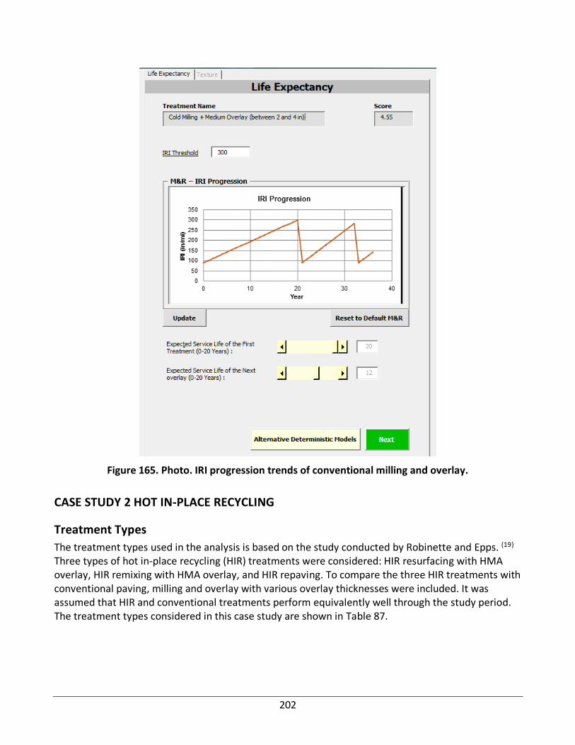
202

Figure 165. Photo. IRI progression trends of conventional milling and overlay.

CASE STUDY 2 HOT IN-PLACE RECYCLING

Treatment Types

The treatment types used in the analysis is based on the study conducted by Robinette and Epps. (19) Three types of hot in-place recycling (HIR) treatments were considered: HIR resurfacing with HMA overlay, HIR remixing with HMA overlay, and HIR repaving. To compare the three HIR treatments with conventional paving, milling and overlay with various overlay thicknesses were included. It was assumed that HIR and conventional treatments perform equivalently well through the study period. The treatment types considered in this case study are shown in Table 87.

203

Table 87. Treatment Type Considered in Analysis

Treatment Number Treatment Type

1 HIR Resurfacing + Thin Overlay (2 inches or less)

2 HIR Remixing + Thin Overlay (2 inches or less)

3 HIR Repaving

4 Cold Milling + Thin Overlay (2 inches or less)

5 Cold Milling + Medium Overlay (between 2 and 4 inches)

6 Cold Milling + Thick Overlay (over 4 inches)

Inputs

In this case study, default values in material, transportation, and construction stage were used. The functional unit is kept as one lane-mile of pavement.

The traffic inputs are as follows: passenger car at 85 percent, small truck at 5 percent, medium truck at 5 percent, large truck at 5 percent, growth rate at 2 percent, and AADT at 4000. The assumptions for work zone traffic control are: speed limited at 60 mph, queue speed 50 mph, work zone speed at 30 mph, and queue length for one mile. Assumptions for end-of-life stage were that 5 percent of pavement materials require landfill with hauling distance of 10 mi and the remaining 95 percent are used for on-site recycling.

Results and Analysis

Table 88 and Table 89 show the total GHG emission and energy consumption of each treatment across all stages from material acquisition to end of life calculated using the IPR tool.

Table 88. GHG Emissions of Each Treatment at Various Stages (Unit: kg CO2 eq.)


Materials Hauling

Construction Use Stage Maintenance End of Life

HIR Resurfacing + Thin Overlay 39,329 41,035 10,175 7,728,901 85,707 876

HIR Remixing + Thin Overlay 39,329 41,035 24,594 7,651,547 85,707 876

HIR Repaving 39,329 41,035 25,030 7,651,547 85,707 876

Cold Milling + Thin Overlay (2 in or less)

37,454 40,611 5,175 7,901,824 128,560 876

Cold Milling + Medium Overlay (2 - 4 inches)

74,908 81,147 6,552 7,838,101 90,228 876


112,362 121,457 5,175 8,368,756 42,853 876

204

Table 89. Energy Consumption of Each Treatment at Various Stages (Unit: MJ)


Materials Hauling

Construction

Use Stage Maintenance

End of Life

HIR Resurfacing + Thin Overlay 717,160 545,680 130,349 38,716,429

2,329,837 61,302

HIR Remixing + Thin Overlay 717,160 545,680 325,138 38,334,031

2,329,837 61,302

HIR Repaving 717,160 545,680 331,128 38,334,031

2,329,837 61,302

Cold Milling + Thin Overlay (2 in or less)

601,731 540,039 63,573 39,543,090

3,494,756 61,302

Cold Milling + Medium Overlay (2–4 in) 1,203,462 1,079,079

82,439 39,221,726

2,321,816 61,302

Cold Milling + Thick Overlay (over 4 in) 1,805,192 1,615,126

63,539 41,746,599

1,164,919 61,302

Figure 167 shows GHG emissions for HIR and conventional overlay treatments in material, hauling, and construction stages. Among the three HIR treatments, the GHG emissions in the material production stage are similar. The differences of GHG emissions are mainly observed in the construction processes. Among the six treatments, conventional milling with thin overlay had the lowest GHG emission. However, conventional milling with thin overlay might not reach the same pavement performance level as HIR treatments. HIR treatments showed environmental benefit of reduction of GHG emission as compared with conventional milling with medium and thick overlay.

Figure 166. Graph. GHG emissions of various treatments from material, transportation, and construction stages.

0E+00

5E+04

1E+05

2E+05

2E+05

3E+05

3E+05

HIR Resurfacing + Thin Overlay (2

in or less)

HIR Remixing + Thin Overlay (2

in or less)

HIR Repaving Cold Milling + Thin Overlay (2

in or less)


(between 2 and 4 in)

Cold Milling + Thick Overlay

(over 4 in)

GH

G E

mis

sio

n (

kg C

O2

eq

.)

Materials Production Materials Hauling Construction

205

Table 90 shows the environmental impacts of various treatments in the material, transportation, and construction stages in a wide range of impact categories, including ozone depletion, smog, acidification, eutrophication, carcinogenic, non-carcinogenic, respiratory effects, and ecotoxicity. Table 91 shows the percent reduction of environmental impacts when treatments of HIR were used instead of conventional mill –and-fill treatment. It is noted that HIR repaving had the highest average environmental impacts compared with HIR resurfacing and remixing. As compared with conventional milling and medium overlay, the average reduction of environmental impacts was 54 percent for HIR resurfacing, 58 percent for HIR remixing, and 58 percent for HIR repaving, respectively.

Table 90. Environmental Impacts for Hot-In-Place Recycling at Various Impact Categories (Material, Transportation, and Construction Stages)

Environmental Impact Categories Unit CIR + Chip Seal

CIR + Thin Overlay

FDR (3 percent FA +1 percent PC) + Medium Overlay


Global Warming kg CO2 eq 9.054E+04 1.050E+05 1.054E+05 1.626E+05

Ozone Depletion kg CFC-11 eq 1.821E-02 2.087E-02 2.094E-02 3.363E-02

Smog kg O3 eq 7.159E+03 7.213E+03 7.215E+03 1.377E+04

Acidification kg SO2 eq 5.604E+02 6.153E+02 6.172E+02 1.037E+03

Eutrophication kg N eq 5.303E+01 6.078E+01 6.105E+01 9.718E+01

Carcinogenic CTUh 1.821E-03 1.989E-03 1.994E-03 3.479E-03

Non-carcinogenic CTUh 1.783E-02 1.784E-02 1.784E-02 3.555E-02

Respiratory Effects kg PM2.5 eq 3.793E+01 4.050E+01 4.057E+01 7.127E+01

Ecotoxicity CTUe 3.411E+05 3.434E+05 3.435E+05 6.776E+05

Fossil Fuel Depletion MJ surplus 4.410E+05 4.686E+05 4.695E+05 8.231E+05

Energy MJ 1.393E+06 1.588E+06 1.594E+06 2.365E+06

Total Energy with Feedstock MJ 3.124E+06 3.319E+06 3.325E+06 5.827E+06

Table 91. Environmental Benefits of Hot-In-Place Recycling Techniques as Compared to Conventional Milling and Medium Overlay

Environmental Impact Categories CIR + Chip Seal (percent)

CIR + Thin Overlay (percent)

FDR (3 percent FA +1 percent PC) + Medium Overlay (percent)

Cold Milling + Medium Overlay (percent)

Global Warming 56 65 65 100

Ozone Depletion 54 62 62 100

Smog 52 52 52 100

Acidification 54 59 60 100

Eutrophication 55 63 63 100

Carcinogenic 52 57 57 100

Non-carcinogenic 50 50 50 100

Respiratory Effects 53 57 57 100

Ecotoxicity 50 51 51 100

Fossil Fuel Depletion 54 57 57 100

Energy 59 67 67 100

Total Energy with Feedstock 54 57 57 100

206

Moreover, the IPR tool considers a full life cycle of pavement including material production, construction, maintenance, use, and end of life. Figure 168 shows the environmental impacts in all stages for each treatment. The results indicate that conventional milling with thin overlay had the highest GHG emissions, while HIR resurfacing, remixing and repaving had similar environmental impacts.

Figure 167. Graph. GHG emissions of HIR treatments in all stages.

Figure 169 through Figure 172 show the IRI progression trends after HIR treatments and conventional milling and overlay, respectively. The study analysis period is 37 years which was calculated automatically by the IPR tool based on the estimated life of different treatments based on multi-criteria performance estimation process.

In this case study, the default IRI projection model was used, which assumes a linear relationship between the initial IRI and the IRI threshold (300 inch/mile) over the service life of pavement. Tables Table 88 and Table 89 show that the HIR treatments had similar environmental impacts in the use stage, while the conventional treatment with thick overlay had the highest GHG emission.

0E+00

1E+06

2E+06

3E+06

4E+06

5E+06

6E+06

7E+06

8E+06

9E+06

1E+07

HIR Resurfacing + Thin Overlay (2 in or less)

HIR Remixing + Thin Overlay (2 in or less)

HIR Repaving Cold Milling + Thin Overlay (2 in or less)

Cold Milling + Medium Overlay (between 2

and 4 in)

Cold Milling + Thick Overlay (over 4 in)

GH

G E

mis

sio

n (

kg C

O2

eq

.)

Materials Production Materials Hauling Construction Use Phase Maintenance End of Life

207

Figure 168. Photo. IRI progression trends of HIR resurfacing.

208

Figure 169. Photo. IRI progression trends of HIR remixing.

209

Figure 170. Photo. IRI progression trends of HIR repaving.

210

Figure 171. Photo. IRI progression trends of conventional milling and overlay.

Summary

Two case studies were conducted using the IPR tool considering three types of rehabilitation treatments: CIR, HIR, and FDR. The results show that for all treatments with most impact categories, the material production stages had the highest environmental impact in the total impact from the three stages of material production, material transportation, and construction. As expected, the recycling treatments had relatively lower environmental impact than the conventional treatment of milling and overlay during the material production and construction life-cycle stages. The findings from case studies provide comparisons of environmental impacts among various rehabilitation treatments and illustrate the basic function of the IPR tool. Although the analysis mainly focuses on material production, transportation, and construction activities, the tool provides the ability to analyze all life-cycle stages such as the use stage, maintenance, traffic delay during construction, and end of life.

a life-cycle methodology for energy use by in-place

Documents