IZA DP No. 1069

A Menu of Minimum Wage Variables forEvaluating Wages and Employment Effects:Evidence from Brazil

Sara Lemos

DI

SC

US

SI

ON

PA

PE

R S

ER

IE

S

Forschungsinstitutzur Zukunft der ArbeitInstitute for the Studyof Labor

March 2004

A Menu of Minimum Wage Variables for

Evaluating Wages and Employment Effects: Evidence from Brazil

Sara Lemos University of Leicester

and IZA Bonn

Discussion Paper No. 1069 March 2004

IZA

P.O. Box 7240 53072 Bonn

Germany

Phone: +49-228-3894-0 Fax: +49-228-3894-180

Email: iza@iza.org

Any opinions expressed here are those of the author(s) and not those of the institute. Research disseminated by IZA may include views on policy, but the institute itself takes no institutional policy positions. The Institute for the Study of Labor (IZA) in Bonn is a local and virtual international research center and a place of communication between science, politics and business. IZA is an independent nonprofit company supported by Deutsche Post World Net. The center is associated with the University of Bonn and offers a stimulating research environment through its research networks, research support, and visitors and doctoral programs. IZA engages in (i) original and internationally competitive research in all fields of labor economics, (ii) development of policy concepts, and (iii) dissemination of research results and concepts to the interested public. IZA Discussion Papers often represent preliminary work and are circulated to encourage discussion. Citation of such a paper should account for its provisional character. A revised version may be available on the IZA website (www.iza.org) or directly from the author.

IZA Discussion Paper No. 1069 March 2004

ABSTRACT

A Menu of Minimum Wage Variables for Evaluating Wages and Employment Effects: Evidence from Brazil

The international literature on minimum wage greatly lacks empirical evidence from developing countries. Brazil’s minimum wage policy is a distinctive and central feature of the Brazilian economy. Not only are increases in the minimum wage large and frequent but the minimum wage has also been used as an anti-inflation policy in addition to its social role. This study estimates the effects of the minimum wage on both wages and employment using panel data techniques and Brazilian monthly household data from 1982 to 2000 at individual and regional levels. A number of conceptual and identification questions is discussed, for example: (1) Various strategies on how to best measure the effect of a constant (national) minimum wage are summarized in a “menu” of minimum wage variables and used to estimate wage and employment effects. (2) An employment decomposition that separately estimates the effect of the minimum wage on hours worked and on the number of jobs is used. Robust results indicate that an increase in the minimum wage strongly compresses the wages distribution with moderately small adverse effects on employment. JEL Classification: J38 Keywords: minimum wage, wage effect, employment effect, informal sector, public sector,

Brazil Sara Lemos Economics Department University of Leicester University Road Leicester LE1 7RH United Kingdom Tel.: +44 116 252 2480 Fax: +44 116 252 2908 Email: sl129@leicester.ac.uk

1

1. Introduction

The aim of minimum wage increases is to change the shape of the wages distribution but not to

destroy jobs. The effect of the minimum wage on other wages is positive because workers bargain to

maintain their relative wages and because firms demand more skilled workers (Sellekaerts, 1981;

Grossman, 1983). Its magnitude varies across the wages distribution because different occupations

have different comparison groups (Grossman, 1983; Akerlof, 1982 and 1984). Elasticities are larger at

lower percentiles, compressing the distribution (Brown, 1999; Card and Krueger, 1995).

There is currently no consensus on the direction of the effect of the minimum wage on

employment. The old debate between the neoclassical Stigler (1946) and the revisionist Lester (1946),

dormant since the early 80s in an apparent consensus, has been re-awakened. The 80s consensus, in

line with standard theory, was of a negative significant but modest effect: increasing the minimum

wage by 10% decreased employment by 1%-3% (Brown, et al., 1982). Neumark and Wascher (1992

and 2000), Deere et al. (1995 and 1996), Currie and Fallick (1996) and Burkahuaser et al. (2000), for

example, estimate negative effects while Card and Krueger (1995 and 2000), Machin et al. (2003),

Machin and Manning (1994), and Dickens et al. (1999), for example, estimate non-negative effects.

Card and Krueger (1995), Ghellab (1998), Cunningham (2002), Saget (2001), and Maloney and

Mendez (2003) discuss some of the international evidence for developing countries. Comparisons

across studies are difficult, not only because of different techniques, data period, and data sources – as

it is also the case in the (mainly US) developed countries literature – but also because the effect of the

minimum wage on wages and employment depends on the minimum wage level (and enforcement) and

on labour market particularities and institutions in each country. The observed wage distribution

compression effect is a lot stronger in Latin America.1 As a result, the employment effect is also

stronger: a 10% increase in the minimum wage (variable) decreases (low wage workers) employment

by up to 12% across the available studies.2 This is substantially larger than the US employment effect.

However, while it is relatively safe to conclude that employment effects are larger in Latin America,

1 See Maloney and Mendez (2003) for empirical evidence across South American countries (Argentina, Bolivia, Brazil,

Chile, Colombia, Honduras, Mexico, and Uruguay), Gregory (1981) and El-Hamidi and Terrell (2001) for Costa Rica, and

Lora and Henao (1997) and Angel-Urdinola (2002) for Colombia. 2 For empirical evidence on Mexico, see Villarreal and Samaniego (1998), Bell (1997) and Feliciano (1998). For Puerto

Rico, see Reynolds and Gregory (1965), Rottenberg (1981), and Castillo-Freeman and Freeman (1992). For Costa Rica, see

Gregory (1981) and Gindling and Terrell (2001). For Chile, see Corbo (1981), Cowan et al. (2003) and Montenegro and

Pages (2004). For Colombia, see Bell (1997) and Maloney and Mendez (2003).

2

care should be taken when referring to their magnitude. This is because there are few point estimates

to rely on, because the variance across the range of estimates is high (due to substantial institutional

differences), and because these estimates might not be directly comparable.

Studies for Brazil, an increase in the minimum wage compresses the wage distribution and has a

small adverse employment effect (Neri, 1997; Carneiro, 2000; Foguel et al., 2000 and 2001; Corseuil

and Morgado, 2001; Corseuil and Carneiro, 2001; Fajnzylber, 2001; Carneiro, 2002; Soares, 2002;

Corseuil and Servo, 2002; McIntyre, 2002; Soares, 2003; Neumark et al., 2003). A 10% increase in the

minimum wage decreases employment by no more than 5%, typically by no more than 1% (not always

statistically significant), across all available studies.3 Using national aggregate data, most of this

literature estimates average wage and employment effects imposing restrictions on time modeling (e.g.

through trends), which does not ensure full identification of the minimum wage effect.

This study estimates the effects of the minimum wage on both wages and employment using panel

data techniques and monthly Brazilian household data from 1982 to 2000 at individual and regional

levels. It represents an important contribution because, further to providing evidence using modern

econometrics techniques in the Brazilian literature, it extends the current understanding on the effects

of the minimum wage in developing countries in the international literature. This study also represents

an important contribution to policymaking, especially after recent South America Governments

promises of minimum wage increases (The Economist, 2002a, 2002b and 2003).

The international literature is poor on evidence outside the US and is greatly lacking on evidence

for developing countries. There are compelling reasons to study the minimum wage outside the US.

“No single empirical study of an economic phenomenon is ever highly convincing” (Hamermesh,

2002, p. 4). Many data points are needed – many and independent data points are needed. Further

empirical evidence is urged for both developed and developing countries – particularly for developing

countries (Hamermesh, 2002). Hamermesh (2002, p. 15) argues for increased reliance on non-US data

and policy evaluations: “policies like hours legislation and the minimum wage provide especially

fruitful areas in which to apply the results of studying foreign experiences to the US”.

Brazil’s minimum wage policy is a distinctive and central feature of the Brazilian economy.

Minimum wage increases in Brazil are large and frequent, unlike the typically small increases studied

in most of the literature (Deere et al, 1996; Hamermesh, 2002; Castillo-Freeman and Freeman, 1992).

3 Dropping the Corseuil and Carneiro (2001) outlier estimate, the employment effect is no more than 3%; dropping the

Corseuil and Morgado (2001) estimate, this effect is no more than 1% across the remaining studies.

3

Studying such increases allows a better possibility of observing the negative effects predicted by

standard theory and thus the link between empirical data and theoretical models of the minimum wage.

Furthermore, Hamermesh (2002) remarks that foreign experiences are especially fruitful if they

generate exogenous shocks, which is the case in Brazil over the past 30 years. Moreover, special

features of the Brazilian Economy are valuable for case studies of the minimum wage, for example: the

minimum wage has been used as an anti-inflation policy in addition to its social role against inequality

and poverty; the public and informal sectors are overpopulated by minimum wage workers; etc. This

unique data is a result of the important role the minimum wage plays in Brazil.

This study uses a number of modern econometrics techniques. (1) It estimates before-and-after

non-parametric Kernel wages distributions to illustrate the minimum wage compression effect. It then

uses regression models to estimate the wage effect across various percentiles of the distribution. (2) It

summarizes various minimum wage variables available in the literature in a “menu” of minimum wage

variables, which are then used to estimate wages and employment effects. (3) It estimates the effect of

the minimum wage on both hours worked and on the number of jobs, and this way, on total

employment. (4) It uses panel data techniques to account for unobserved regional macro fixed effects

separately from the minimum wage effect on employment.

This study is organized as follows. Section 2 describes the data and presents the minimum wage

institutional background (Section 2.1). Section 3 defines minimum wage variables (Section 3.1)

presents wage models (Section 3.2), which motivate a discussion on identification (Section 3.3.1) and

model re-specification (Section 3.3.2). Section 4 presents the decomposition of total employment

effects into hours and jobs effects (Section 4.1), employment models (Section 4.2) and robustness

checks (Section 4.3 and 4.4). Section 4.5 discusses the evidence and Section 5 concludes. Robust

results indicate that an increase in the minimum wage strongly compresses the wages distribution with

moderately small negative effects on employment.

2. Data

The data used is Pesquisa Mensal do Emprego, a monthly household survey similar to the US

Current Population Survey. Between 1982 and 2000, PME collected over 21 million observations

across the six main Brazilian metropolitan regions: Bahia (BA), Pernambuco (PE), Rio de Janeiro (RJ),

Sao Paulo (SP), Minas Gerais (MG) and Rio Grande do Sul (RS). Its monthly periodicity is important

because wage bargains during the sample period occurred annually, bi-annually and monthly (Section

4

2.1). Comparisons of demographic and economic characteristics across regions and waves show no

selectivity bias in any direction (Neri, 1996). The deflator, INPC (National Consumers Price Index),

was regionally disaggregated to reduce measurement error. All data is available from the Instituto

Brasileiro de Geografia e Estatistica.

Graph 1 plots the real minimum wage and the average, 25th, 50th, and 75th percentiles of the wages

distribution over time. A visual inspection suggests that the minimum wage is more strongly correlated

with lower percentiles; this is confirmed by correlations in the national aggregate of 0.78 and 0.73 for

the 25th and 75th percentiles (Graphs 1.b and 1.d). Such correlations for PE and SP are respectively

0.95 and 0.36, and 0.78 and 0.55, which illustrate large regional variation.

Graph 2 plots log employment rate against log real minimum wage. A visual inspection suggests a

non-negative association between the two. The positive correlation in levels fades as the data is

differenced; this is confirmed by correlations of 0.181, 0.054, 0.211 and -0.005, respectively in levels,

first-difference, twelfth-difference, and both first and twelfth differences. Such correlations for PE and

SP in levels are respectively 0.37 and 0.01, which again illustrate large regional variation.

2.1 Minimum Wage

The minimum wage was introduced in 1940 as a social policy to provide subsistence income (diet,

transport, clothing, and hygiene) for an adult worker. The associated bundle varied across regions,

which was reflected in 14 minimum wages – the highest (lowest) for the Southeast (Northeast)

(Gonzaga and Machado, 2002). Wells (1983, p. 305) believes they were “generous relative to existing

standards” since about 60% to 70% of workers earned below them; Saboia (1984) and Oliveira (1981)

believe they legitimated the low wages of the unskilled. Regional minimum wages existed until 1984

when a single national minimum wage was introduced. Coverage is full; there is no legal sub-

minimum or differentiated minimum wage rates for specific demographic groups or labour market

categories.4

After a steep decrease, the real minimum wage was adjusted and reached its peak during the boom

of the 50s, when productivity was high, unions strong, and the Government populist. After that, it

decreased as a result of the subsequent recession, rising inflation, and non-aggressive unions (Singer,

1975). The real minimum wage was then 40% lower than in the 50s. The dictatorship installed in

4 Up to 70% of the minimum wage can be deducted to pay for accommodation and food costs. This accounts for some

below minimum wage workers, although most of those are informal sector workers.

5

1964 associated high inflation with wage adjustments and limited labour organization, reduced wage

militancy, and implemented a centralized wage policy. One of the strategies of this policy was under-

indexation of the real minimum wage, which transformed it “from a social policy designed to protect

the worker’s living standard into an instrument for stabilization policy” (Camargo, 1984, p.19). The

“Teoria do Farol” (Lighthouse Effect) associated the subsequent increase in inequality revealed in the

1970 Census with the pos-64 real minimum wage decrease (Souza and Baltar, 1979, 1980; Macedo and

Garcia, 1978 and 1980).

According to Carneiro and Faria (1998), the nominal minimum wage was used not only as a

stabilization policy but also as a coordinator of the wage policy. One example is that other wages were

set as multiples of the minimum wage. Another example is that in the early 80s, wages between 1 and

3 times the minimum wage were bi-annually adjusted by 110% of the inflation rate (Cascade effect);

the higher the worker’s position in the wage distribution, the lower the percentage adjustment. Such

increases immediately spilled over higher up in the wage distribution. In the presence of high inflation

and distorted relative prices, rational agents took increases in the minimum wage as a signal for price

and wage bargains (Gramlich, 1976; Card and Krueger, 1995; Freeman, 1996) – even after law forbade

its use as numeraire in 1987. Maloney and Mendez (2003) and Marinakis (1998) show that the

Lighthouse and numeraire effects are a general phenomenon in Latin America.

The real minimum wage was under-indexed not only because it was associated to high inflation

but also because of its impact on the growing public deficit via benefits, pensions, and the Government

wage bill.5 This impact has often been the criterion for the affordable increase in the nominal

minimum wage, resulting in under-indexation of the real minimum wage (Foguel et al., 2001).

Thus, because of its effects both on prices and on the public deficit, the real minimum wage was

under-indexed and used as a deflationary policy. However, when pressure was enough, the

Government had to give in, allowing increases in the nominal minimum wage – the nominal minimum

wage became the “messenger” of the inflation – which in turn severely affected both prices and the

public deficit and were therefore inflationary. This effect was perpetuated into an inflation spiral. In

this context, the minimum wage has been alternately used as social and anti-inflation policy. The

policy choice depended on the level of inflation, on the workers bargaining power, and on the

Government party affiliation (Velloso, 1988; Bacha, 1979). The social role is associated with more

populist Governments, lower inflation, and stronger unions.

5 In the sample period, 12% of the population are pensioners, 7% are civil servants.

6

Graph 1.a shows that the hourly real minimum wage decreased between 1982 and 2000.6 Its

highest (lowest) level was in November 1982 (August 1991), before the acceleration of inflation. In

political terms, three events were important in the 80s: (a) in 1984, the minimum wage became

national, after slow regional convergence; (b) with the end of the military regime in 1985, the 1988

Constitution re-defined the subsistence income (diet, accommodation, education, health, leisure,

clothing, hygiene, transport, and retirement) for an adult worker and his/her family – even though such

a bundle was unaffordable at the prevalent minimum wage; (c) the union movement re-emerged and

became ever stronger, reaching a high union density for a developing country (Carneiro and Henley,

2001; Amadeo and Camargo, 1993). In economic terms, despite the political changes, the minimum

wage was still a component of the centralized wage policy. The 80s and 90s witnessed an exhausting

battle against inflation. Five stabilization plans between 1986 and 1994 had different nominal

minimum wage indexation rules depending on the inflation level. These indexation rules resulted in

the saw-toothed pattern in the real minimum wage shown in Graph 1.a; nominal minimum wage

increases were large and frequent, but quickly eroded by the subsequent inflation. Since then, under

reasonably stable inflation, the minimum wage has not been explicitly used as an anti-inflation policy.

3. The Minimum Wage Effect on the Wage Distribution

3.1 Minimum Wage Variables

The most common way to relate the minimum wage to other wages in the literature is to use the

ratio of the minimum wage to average wage adjusted for coverage of the minimum wage – the Kaitz

index (Kaitz, 1970). The Kaitz index also received the intuitive name of “toughness” of the minimum

wage (Machin and Manning, 1994). Graph 3.a shows log toughness, whose the correlation with the log

real minimum wage in the national aggregate is 0.81. Baker et al. (1999) also found the ratio to have a

similar path to that of the minimum wage for Canada; Dickens et al. (1999) for the UK, and Card and

Krueger (1995) for the US. While the Kaitz index was 0.39 for the US and 0.40 for the UK in 1993

(Dolado et al., 1996), it was 0.27 for Brazil, although as high as 0.45 in PE, which is a poor region.

Similarly, the ratio of the minimum wage to the median and also to the 25th percentile of the wage

distribution are defined as log toughness 50 and log toughness 25. On the one hand, log toughness 50

6 The hourly minimum wage rate is obtained by dividing the monthly minimum wage by 44*4.3 after, and 48*4.3 until

September of 1988, because the new Constitution shortened the working week. The hourly wage rate is obtained by

dividing the monthly earnings by the number of hours worked in the week before the interview multiplied by 4.3.

7

is a better central measure of the distribution if wage inequality is substantial as in Brazil (Bacha, 1979;

Fernandes and Menezes-Filho, 2000), in which case the average fails to be representative of most

people (who are at the bottom). The correlation with the log real minimum wage in the national

aggregate is 0.81. On the other hand, the minimum wage affects the low, not the average or median

wage worker (Deere et al., 1996). This is confirmed by the 0.80 correlation of log toughness 25 with

the log real minimum wage in the national aggregate (see Graph 3.b).

Graph 3 also plots other minimum wage variables suggested in the literature. They are called

“degree of impact” measures (Brown, 1999), because they focus on the proportion of workers directly

affected by increases in the minimum wage. Graph 3.c shows “fraction affected”, i.e. the proportion of

people earning a wage between the old and the new minimum wage (Card, 1992; and Card and

Krueger, 1995),7 whose correlation with the log real minimum wage in the national aggregate is 0.57.

While the fraction affected was 7.4% for the US in 1990 (Card and Krueger, 1995), it was 8% for

Brazil, although as high as 49% in PE. Because fraction affected is zero when the nominal minimum

wage is constant, fraction was also defined using real data. Graph 3.d shows that “fraction real” has

more variation, although a lower correlation with the log real minimum wage in the national aggregate

(0.49), than fraction affected because the real minimum wage was never constant in the sample period.

A measure closely related to fraction is the spike in the wages distribution generated by the

minimum wage (Card and Krueger, 1995; Brown, 1999). Graph 3.e shows “spike”, i.e. the proportion

of people earning one minimum wage (Dolado et al., 1996), whose correlation with the log real

minimum wage in the national aggregate is 0.64. Spike moves in response to the minimum wage,

being bigger after an increase and smaller as different categories negotiate their salaries and pull out of

the minimum wage (Card and Krueger, 1995). This is particularly the case if inflation is high and the

minimum wage is constant (Carmargo, 1984). Note the corresponding saw-toothed pattern in Graph

1.a, also documented by Brown (1999) for the US. Whereas Graph 3.e shows spike over time for the

full sample, Graph 4 shows the actual spike in the earnings distribution for PE for each month of 1992

(the vertical line is the minimum wage). While the spike was 4% for the US in 1993 (Dolado et al.,

1996), it was 12% for Brazil, although as high as 25% in PE.8

7 The old minimum wage is multiplied by 0.98 and the new minimum wage, by 1.02 to account for rounding

approximations. This procedure was used for all degree of impact measures here defined. 8 As in Graphs 4 and 5, spike is here defined using real earnings as opposed to real hourly wages used elsewhere in this

study. The monthly definition produces larger spikes because workers who earn one monthly minimum wage but work

shorter (longer) hours than the typical working week, will earn above (below) one hourly minimum wage. It can be argued

8

Because of the minimum wage numeraire and indexer roles in Brazil (Section 2.1), Gonzaga et al.,

(1999) expanded spike to embrace those earning not only one, but also 0.5, 1, 1.5, 2, 2.5 and 3 times

the minimum wage. Graph 3.f shows “multiples”, whose correlation with the log real minimum wage

in the national aggregate is 0.31. Figures almost as large as 20% are observed when Plano Cruzado

and Plano Real were implemented (spike, fraction and percentage (below) are also large in both

events). Neri (1997) suggested multiples as an appropriate variable to test the Lighthouse effect

(Section 2.1), which amounts to testing for spillover effects.

A related measure is the proportion of people earning the minimum wage or below (Dolado et al.,

1996). Graph 3.g shows “spike and below”, whose correlation with log real minimum wage in the

national aggregate is 0.77. Note the resemblance with the minimum wage itself (Graph 1.a). A

noteworthy figure of 44% is observed in the early 80s in BA, which is a poor region.

The numeraire role, together with the Lighthouse effect (Section 2.1), motivated Foguel (1997)

and Gonzaga et al. (1999) to define a measure of the effect of a minimum wage increase across the

wage distribution. Graph 3.h shows “percentage”, i.e. the proportion of people whose wages were

increased by the minimum wage percentage increase (regardless of their position in the distribution),

whose correlation with the log real minimum wage in the national aggregate is 0.39. As multiples,

percentage is a measure of spillover effects.

3.2 Descriptive Wage Models

The compression in the earnings distribution following a minimum wage increase is illustrated by

estimating non-parametric Kernel distributions before and after the wage increase. Graph 5 plots

superimposed distributions which show the change in the shape of the distribution after minimum wage

increases in May, September and January of 1992. Just as an increase makes the distribution less

dispersed, a decrease (in the remaining months the real minimum wage was inflation eroded) makes it

that using variables in hourly terms to model a labour market operating on a monthly basis might introduce measurement

error. The correlation between the monthly and the hourly definitions of each variable is high and the estimation results are

robust to either definition. Furthermore, hourly definitions ensure that the results are consistent with theory and comparable

with the existing empirical literature (the minimum wage rate is an hourly rate in most countries for which empirical

evidence is available). Moreover the hourly definition plays a crucial role when defining the employment decomposition in

Section 4.1.

9

more dispersed. This can be formalized by estimating the effect of the minimum wage at various

percentiles across the distribution controlling for the effect of other variables on wages.

The simplest model of wages as a function of the minimum wage is:

irtw

rtww

irt urMWrwage ++= loglog βα ,

where irtrwage is real wages, rtrmw is real minimum and wirtu is the error term for individual i in

region r in time (month) t . This model can be aggregated for the mean and, for a more complete

picture, also for the 5th, 10th, 15th, 20th, 25th, 30th, 35th, 40th, 45th, 50th, 90th, and 95th percentiles of the

wage distribution. In this fashion, the effect of the minimum wage at various points across the

distribution is estimated (Dickens et al., 1999).

Region and time dummies were included to model region and time fixed effects. Region dummies

separate regional effects and time dummies separate other macro variable effects from the effect of the

minimum wage on wages. A macro variable explicitly included is past inflation. This is because, on

the one hand, the macroeconomic policy, including the minimum wage policy, was aimed at stabilizing

the inflation; thus, inflation is driving other variables. On the other hand, the minimum wage was used

as indexer (Section 2.1); thus, past inflation captures the portion of the minimum wage increase that

merely compensates for past inflation. Another macro variable explicitly included is the unemployment

rate, typically used as a measure of demand for labour to control for region specific macro shocks that

might be correlated with the minimum wage (Card and Krueger, 1995; Brown, 1999). The new

equation (after aggregation) is:

wrt

wt

wrrt

wrt

wrt

wwrt uffuratelationrMWrwage ++++++= − δγβα 1infloglog (1)

The standard neoclassical model underlies the above empirical equation. Assume perfect

competition on the input and output markets, and a production function Y depending on skilled and

unskilled labour, with input and output prices W, MW, and p. Maximization of profits at the

(representative) firm level delivers the aggregate demand function for (skilled or unskilled) labour,

Ld=L(p,W,MW), which is the theoretical ground for the employment equation in Section 4; all prices

are normalized by W, and employment is modeled as a function of toughness and inflation (Card and

Krueger, 1995). The demand function can be rewritten as W=W(p,L,MW), which is the theoretical

ground for the wage equation above; wages are modeled as a function of the minimum wage, inflation

and unemployment rate.

10

Given the labour demand, if labour supply is positively sloped, some sort of reduced form is what

is being estimated, and supply shifters need to be included. The following variables are included to

control for region specific demographics potentially correlated with the minimum wage, namely, the

proportion of workers in the population who are: young, younger than 10 years old, women, illiterates,

retired, students, in the informal sector, in urban areas, in the public sector, in the building construction

industry sector, in the metallurgic industry sector, basic education degree holders, high school degree

holders, and the proportion of workers with a second job.9 The new equation is:

'1infloglog w

rtw

tw

rwrt

wrt

wrt

wrt

wwrt uffcontrolsuratelationrMWrwage +++++++= − λδγβα (1’)

The model was estimated in levels and in first-differences. Time and regional dummies, past

inflation, controls and the constant were included in the model in levels and in the model in differences.

In the later, these were included after differencing – i.e. the constant is the base dummy (not a trend

from the model in levels) and the regional dummies model region specific trends. The models were

sample size weighted to account for the relative importance of each region (and for heteroskedasticity

arising from aggregation) and White-corrected; the models in levels were corrected for serial

correlation specific to each region (Dolado et al., 1996; Zavodny, 2000).

The two first columns of Table A (in the appendix) show robust and significant estimates, more

robust for lower percentiles and for models in levels. An increase in the minimum wage affects the

10th percentile 10 times more than the 90th percentile of the wages distribution (model in differences).

A 10% increase in the minimum wage is associated with a wage increase of 5.53% (3.56%) for those in

the 10th (30th) percentile. This is the counterpart of the compression effect in Graph 5. Equations (1)

and (1’) can be re-estimated using percentile ratios and the standard deviation of the wage distribution

as dependent variables regressed on the same set of regressors as above to check further the

9 There is some agreement that demand side variables should be held constant, but less agreement on whether supply side

variables should be included as controls and, if so, which ones. The debate is about whether a reduced form or a demand

equation is estimated, depending on whether the minimum wage is binding or not (Neumark and Wascher, 1992 and 1996).

Typically, employment equations in the literature have been interpreted as demand equations, even though many include

supply side variables (Card and Krueger, 1995). Particularly debatable is the inclusion of a variable measuring enrolment

rates at school (Card and Krueger, 1995; Neumark and Wascher, 1992). If minimum wage reduces both employment and

enrolment, reduced form and enrolment rate constant employment equations have very different interpretations (Brown,

1999). In Brazil, a large number of minimum wage workers are adults no longer at school. Also, schooling is largely

available outside working hours, and therefore working and schooling need not be exclusive alternatives; if present, the

11

compression effect. The results in Table A show that an increase of 10% in the minimum wage

decreases the 50th-10th percentile gap by 3.47%, the 90th-10th gap by 5.04%, and the 90th-50th gap by

1.56%. Neumark et al (2003), Soares (2002), Fajnzylber (2001), Corseuil and Morgado (2001) and

Corseuil and Carneiro (2001) also found evidence of a compression effect for Brazil. Dickens et al.

(1999) and Card and Krueger (1995) found similar evidence for the UK and the US.

3.3 Wage Model Re-Specification

3.3.1 Identification

The effect of the minimum wage on wages would be fully identified in Equations (1) and (1’) if

the nominal minimum wage had regional variation in Brazil. In that case, no restriction on time

modeling would need to be imposed, i.e. a full set of time dummies could be used to model time

effects. However, as the nominal minimum wage is constant across regions – any variation across

regions in the real minimum wage stems from the variation in the regional deflators – a full set of time

dummies cannot be used and some restriction needs to be imposed on modeling time effects (e.g.

through time trends). In this case, the effect of the minimum wage on wages is not fully identified

because the estimate is sensitive to the particular restriction imposed.

To circumvent this empirical problem, various minimum wage variables with regional variation

have been suggested in the literature. The most common variable has been toughness; others are:

fraction, spike and below, spike, multiples, and percentage, as defined in Section 3.1.10 The idea here

is to collect all these variables in a “menu” of minimum wage variables and to compare their estimates.

Confidence will be greater if the results are robust across variables.

Although such “degree of impact measures” have variation across regions, a full set of dummies

still eliminates all the variation in the model, because minimum wage increases are systematic

(Burkhauser et al., 2000). If on the one hand month dummies eliminate all the variation, on the other

hand year dummies alone are not sufficient to model time in a month model. An alternative is a hybrid

simultaneity bias will not be as severe. Due to these particularities and the unresolved debate, enrolment rate was not here

included (Williams, 1993; Baker, 1999). 10 Lee (1999) and Green et al. (2001) suggested trimmed toughness; Deere et al. (1996) suggested costs of the increase on

the firm’s side; and various authors suggested some variation of a wage gap measure (Linneman, 1982; Deere at al., 1996;

Currie and Fallick, 1996).

12

model, where seasonal-month dummies are included in addition to year dummies, to control for

unobserved fixed effects across months, as in Burkhauser et al. (2000). Also, stabilization plan

dummies11 are included to capture common macro shocks under each stabilization plan.

3.3.2 Re-Specification

Thus, the minimum wage variables defined in Section 3.1, namely fraction, fraction real, spike,

spike and below, multiples and percentage, are each used in turn as a “proxy” to the real minimum

wage in Equations (1) and (1’). Table A (in the appendix) shows estimates more robust and larger at

lower percentiles. At higher percentiles, they are not only smaller but also sometimes not significant,

suggesting no spillover effects higher in the distribution.

The estimates show a very similar pattern whatever minimum wage variable is used. The fraction

estimate, before the inclusion of controls, is 1.202 (0.908) for those in the 10th (30th) percentile of the

wages distribution. In other words, an increase in the minimum wage sufficient to increase fraction by

1 percentage point is associated with an increase in the wages of those in the 10th (30th) percentile of

the wages distribution of 1.20% (0.91%). A 10% increase in the nominal minimum wage increases

fraction by 3.7 percentage points12 and is associated with an increase in the wages of those in the 10th

(30th) percentile of 4.45% (3.36%). Card and Krueger (1995) found estimates between 0.18 to 0.30

using a similar specification, here comparable with 0.52 (Panel B of Table A). Adding demographic

controls affects only marginally the magnitude of the estimates, and does not affect their sign or

significance. These figures are respectively 1.401 (1.072) for fraction real;13 1.821 (0.954) for spike

and below; 3.659 (1.034) for spike; 0.657 (0.220) for multiples; and 2.868 (2.391) for percentage.

Neumark et al. (2003) found 0.45 (-1.68) estimates for the 10th (30th) percentile of the formal sector

11 Each had very particular rules (Abreu, 1992); macro shocks were similar within, and different across plans. Additionally,

a dummy was defined in October 1988, when the new Constitution: shortened the working week from 48 to 44 hours, and

introduced an alternative working day of 6 consecutive hours instead of 8 hours with a lunch break. 12 This was obtained by regressing the difference of fraction on the difference of the log of nominal minimum wage and

controls associated to each equation. However, because the nominal minimum wage does not vary across regions (Section

3.4.1), log toughness, log toughness 50 and log toughness 25 were also used. A 10% increase in the minimum wage

increases fraction by 3.7 percentage points, fraction real by 1.4, spike and below by 1.8, spike by 0.3, multiples by 0.4, and

percentage by 0.5. These estimates were remarkably robust across specifications.

13

wage distribution in Brazil between 1996 and 2001 (low inflation period) using not the proportion of

workers at the spike and below, but the proportion of workers “below spike”. A preferred specification

is not chosen; instead, the range of estimates produced across all specifications is expected to embrace

the true coefficient. Table 1 presents the interval that brackets the effect of a 10% increase in the

minimum wage across models and variables. A 10% increase in the nominal minimum wage is

associated with an increase in the wages of those in the 10th (30th) percentile of 0.23%-6.35% (0.06%-

4.61%) across models. Tables 1 and A also show percentile ratios and standard deviation regressions

that confirm the compression effect reported in Section 3.2.

The spillover effects are now weaker than in Section 3.2. Extensive spillovers are expected in

Brazil because of the minimum wage indexer and numeraire roles (Section 2.1), and for Latin America

in general (Maloney and Mendez, 2003). However, the extensive spillovers in Section 3.2 might result

from artificial correlation between the real minimum wage and real wages, driven by the common

(deflator) denominator. Therefore, more weight should be put in the spillover estimates using the

“degree of impact measures”.

The effect of the minimum wage on the wage distribution was here exhaustively measured using a

variety of specifications and variables. Initially, the mean, median, various percentiles, their ratios, and

the variance of the wage distribution were modeled as a function of the minimum wage. Then such

models were re-specified using various alternative minimum wage variables defined to capture

differently the effect of the minimum wage on the wage distribution: at, below and above the minimum

wage, as well as across the distribution. All the above pieces of evidence consistently suggest that the

minimum wage compresses the wage distribution.

4. The Effect of the Minimum Wage on Employment

4.1 Decomposition of the Total Employment Effect

Employment can be adjusted in two margins following a minimum wage increase: the number of

posts of jobs and the number of hours of work. As a result, the total effect of a change in the minimum

wage on employment can be decomposed into hours and jobs effect. If the first is positive and the

second is negative, the total employment effect might be non-negative. This might offer an explanation

13 Fraction real was interacted with a dummy for real minimum wage increases because a decrease might not have such as

severe an impact (wages are sticky), i.e. an increase is expected to affect the wage distribution more. However, the data did

not show enough variation to reject the null hypothesis.

14

for the clustered-around-zero employment effect found in the literature. Although this issue has not

received much attention (Barzel, 1973; Gramlich, 1976; Linneman, 1982; Brown et al., 1982; Brown,

1999), more recent research (Michl, 2000; Zavodny, 2000; Card and Krueger, 2000; Neumark and

Wascher, 2000) suggests that non-negative effects on jobs are a sub-product of adjustments in hours.

Zavodny (2000), Machin et al. (2003) and Neumark et al. (2003) estimate job and hours effects, but do

not formalize it as a decomposition.

Let average hours in the population (T ) be equal to the product of average hours for those

working ( H ) and the employment rate ( E ), EHT = is NN

N

hour

N

houre

e

N

eii

N

ii ∑∑

∈= =1

, where eN and N are

sample sizes of the employed and working population and hour is hours worked. As noted by Brown

et al. (1982, p. 497), “to measure the employment effect of the minimum wage, the ratio of

employment to population [ E ] is used most often as the dependent variable”. However, the above

decomposition suggests not only E , but also T and H as dependent variables. Because of that,

Equation (2) in Section 4.2 is estimated separately using each of the three employment variables E , T

and H in turn as a dependent variable. Assuming a log-log form and using the same set of regressors

in each one of the three equations, the additivity property of OLS holds and the estimate of the real

minimum wage in the T equation equals the sum of the estimates of the real minimum wage in the

H and E equations, i.e. eE

eH

eT βββ += .

4.2 Descriptive Employment Models

The simplest model of employment as a function of the minimum wage is:

ert

et

errt

eert uffrMWemployment ++++= loglog βα (2)

where rtemployment is in turn E , T or H ; rtrmw is real minimum wage as before, erf and e

tf are

regional and time fixed effects (Section 3.3.1); and ertu is the error term. This equation was then re-

estimated including the same controls as in Section 3.1 The new equation is:

'1infloglog e

rte

te

rrte

rrte

rtee

rt uffcontrolslationrMWemployment ++++++= − λγβα (2’)

This equation was also re-estimated including dynamics in the form of 24 lags of the dependent

variable. This is because an increase in the minimum wage might not affect employment

15

contemporaneously, but in future periods (Brown et al., 1982; Hamermesh, 1995).14 The new equation

is:

∑=

−− +++++++=24

1

''11 loginfloglog

l

ert

et

errt

el

ert

ert

ert

eert uffemploymentcontrolslationrMWemployment ρλγβα (2’’)

Each specification was estimated for four alternative data filters: levels, first-difference, twelfth-

difference, and both first and twelfth differences. This is to account for Baker et al.’s (1999) criticism

that negative or positive employment effects are found depending on whether short or long differencing

is used. As discussed in Section 3.1, dummies, past inflation and constant were included after

differencing; the models were White-corrected and sample size weighted. The errors were assumed to

be serially uncorrelated over time. Ultimately, an orthogonality condition must be made to produce an

estimable equation and it is not too unrealistic to assume that serial correlation over time will vanish

after differencing, adding dynamics, controls, regional and time dummies.

Recall Graph 2 that plots log employment rate ( E ) against log real minimum wage ( rMW ). As

discussed in Section 2, the plots and correlations suggests a non-negative association between the

minimum wage and employment rate. Graph 6 and corresponding Panel I of Table B (in the appendix)

show total effect, hours effect and jobs effect estimates, mostly not significant. The total effect

estimates are positive because they are dominated by the hours effect (Brown, 1999). A 10% increase

in the minimum wage is associated with a 0.01% increase in total employment in the model in levels

with dynamics (column 3 of Table B), decomposed into 0.03% increase in the number of hours worked

(lighter bars) and 0.04% decrease in the number of posts of jobs (darker bars).15 In the long run, total

employment increases by 0.01% (column 4 of Table B). A 10% increase in the minimum wage is

associated with a decrease in total employment of 0.09% (0.07%) at the most (across all estimates) in

the short (long) run. Neumark et al. (2003) estimates small negative but not always significant hours (-

0.9%) and jobs (-0.6%) effects for Brazil using formal sector data in low inflation period, when more

adverse employment effects are expected (Section 4.5).

4.3 Employment Model Re-Specification

As in Section 3.3.2, the minimum wage variables defined in Section 3.1, namely fraction, fraction

real, spike, spike and below, multiples, percentage, log toughness, log toughness 50, and log toughness

14 Employment is AR(2) using annual data (Layard et al., 1991), which is equivalent to 24 lags on monthly data. 15 Because in dynamic models the set of regressors is not the same, the OLS additivity property does not hold exact.

16

25, are each used in turn as a “proxy” to the real minimum wage in Equations (2), (2’) and (2’’). Table

B shows estimates mostly statistically different from zero. Panel II – FRACTION shows that the total

employment estimate ranges from -0.005 to 0.045. In other words, an increase in the minimum wage

sufficient to increase fraction by 1 percentage point is associated with a decrease in total employment

of 0.005% at the most. As discussed in Section 3.3.2, a 10% increase in the minimum wage (increases

fraction by 3.7 percentage points) is associated with a decrease in total employment of 0.017% at the

most. Card and Krueger (1995) found estimates between 0.03 to 0.36 when regressing the change of

employment-population ratio on fraction, which lies in the range -0.016 and 0.001 of jobs effects

estimate (Panel II of Table B). Panel III – FRACTION REAL shows 0.008 to 0.041; Panel IV – SPIKE

AND BELOW, -0.074 to 0.347; Panel V – SPIKE, -0.036 to 0.779; Panel VI – MULTIPLES, -0.031 to

0.068; Panel VII – PERCENTAGE, -0.008 to 0.127; Panel VIII- TOUGHNESS, 0.011 to 0.066; Panel IX –

TOUGHNESS 50, 0.005 to 0.055; and Panel X – TOUGHNESS 25, 0.016 to 0.072. The largest and most

robust estimates are for spike and spike and below. Finally, the last two columns of Table B show a

long run estimate no bigger than -0.117 across models.

Table 2 presents the interval that brackets the effect of a 10% increase in the minimum wage

across models and variables. The total employment effect ranges from -0.95% to 1.40%, decomposed

into the hours coefficient ranging from -0.01% to 1.81% and the jobs coefficient ranging from -0.73%

to 0.28%. Once more, the total employment effect appears to be dominated by the hours effect

(Brown, 1999). In the long run, a decrease in total employment is no bigger than 0.67%.

The range of estimates produced across all specifications and variables is expected to embrace the

true coefficient. The preferred specification is the one in first differences using spike as a minimum

wage variable – i.e., column 3, row 2, Panel V of Table A. This specification is expected to produce

errors serially uncorrelated, and spike can be argued to be a better minimum wage variable.16 Also,

spike models produced some of the largest and most robust estimates, conforming to a more cautious

16 Spike is an alternative to toughness and fraction, the most common minimum wage variables in the literature. Toughness

varies across regions and over time, but the criticism in Section 3.3.1 applies. Brown (1999) compares the ‘degree of

impact’ measures (for example, fraction) and the ‘relative minimum wage’ variable (for example, toughness) and concludes

that the former are conceptually cleaner although not well suited for studying periods when the minimum wage is constant.

That is because fraction is constant at zero regardless of how unimportant the minimum wage might become. On the one

hand spike is conceptually related to fraction and is therefore methodologically clean; on the other hand spike does not

suffer from the same drawback, as it can be defined even when the minimum wage is constant. Beyond statistical

identification, spike is a measure of those workers becoming more expensive, i.e. a measure of the extra employment costs,

and therefore well suited to study minimum wage employment effects.

17

approach. Thus, this specification is more reliable both conceptually and statistically; it is also more

comparable with specifications in the existing literature, mostly in first differences. Incidentally this

preferred specification produces estimates fairly similar to the other specifications.

Bracketing the total employment effect below 1% across such a variety of models is reassuring.

The total effect appears to be dominated by the hours effect. This suggests that the minimum wage

does not hurt as much where it hurts the most: causing disemployment. The employment effect was

here exhaustively measured and was remarkably robust to various alternative specifications and

minimum wage variables. This is in line with the international and Brazilian literature and in line with

prior expectations discussed in Section 1. All the above pieces of evidence suggest that an increase in

the minimum wage does not always have a significant effect on employment and it is not always

negative; a cautious reading is that the minimum wage has a moderately small negative effect on

employment.

4.4 Alternative Employment Model Re-Specifications

It can be argued that the degree of impact measures are an imperfect “proxy” and do not capture all

the relevant variation in the real minimum wage, introducing measurement error and possibly omitted

variable bias. An alternative specification, is to include the interaction of the degree of impact

measures with the real minimum wage to check the robustness of the estimates in Section 4.3. As

argued in Section 4.3, spike is regarded as the preferred minimum wage variable. Thus, Equations (2),

(2’) and (2’’) were re-specified as follows:

ert

et

errtrt

emsrt

esrt

em

ert uffspkrMWspkrMWemployment ++++++= logloglog βββα (3)

+++++= − rrte

rtrtemsrt

esrt

em

ert lationspkrMWspkrMWemployment 1inflogloglog γβββα

'ert

et

errt

e uffcontrols ++++ λ (3’)

+++++= − rrte

rtrtemsrt

esrt

em

ert lationspkrMWspkrMWemployment 1inflogloglog γβββα

∑=

− +++++24

1

''1log

l

ert

et

errt

el

ert

e uffemploymentcontrols ρλ (3’’)

18

As in Section 4.2, each specification was estimated for four alternative data filters: levels, first-

difference, twelfth-difference, and both first and twelfth differences. Spike (appearing on its own and

on the interaction term) was included in levels in all specifications, or put differently, spike was

included after differencing. Similarly, dummies, past inflation, controls and the constant were included

after differencing. The models were White-corrected and sample size weighted. The errors were again

assumed to be serially uncorrelated over time.

Table C shows estimates for the spike and for the interaction term. The pattern of magnitude,

signs and significance of the spike estimates (see Panel I of Table C) is remarkably similar to the spike

estimates prior to including the interaction term (see Panel V of Table B). The estimates of the

interaction term were mostly not statistically significant (see Panel II of Table C). That is because the

interaction term does not have regional variation over and above the variation that spike already

captures. Although the interaction term has variation across regions and over time, the extra variation

is mainly over time and, as argued in Section 3.3, the crucial variation that identifies the minimum

wage effect is across regions. Furthermore, whatever additional regional variation brought in by the

real minimum wage is due to variations in the deflator, and therefore does not help to identify the

coefficient (Section 3.3). This is a data problem, because the nominal minimum wage is constant in

Brazil. If spike was interacted with the nominal, instead of the real minimum wage, month time

dummies would absorb all the additional time variation brought in by the nominal minimum wage.

These re-specifications are more demanding than the specifications in Section 4.3. It is therefore

very reassuring that the results are robust do not change the previous conclusions.

4.5. Further Employment Effects Evidence

The main message in this study is that wage effects in Brazil are large whereas employment effects

are small. Despite of the large minimum wage increases; despite of the large proportion of minimum

wage workers at the minimum wage directly affected by these increases; and despite of the large

proportion of workers below and above the minimum wage, indirectly affected by these increases via

spillovers; the employment effects in Sections 4.2 to 4.4, although in line, are small when compared

with the -1% effect in the international literature.

Beyond robustness checks to ensure statistical identification, robustness checks focusing on

underlying specificities in the Brazilian Economy might offer explanations for such small effects.

Evidence on employment effect on key sub-samples is here reviewed as a further check of the

19

robustness of the above employment effects. Although the evidence considered shed some light as to

why employment effects are small for Brazil, uncovering the a priori expected more negative

employment effect proved difficult.

The reading of the evidence considered here is that small employment effects might be sensible

when a number of explanations are combined. For example, employment effects are not easy to find if

non-compliance is large and the public sector has an inelastic labour demand. Additionally,

employment effects are difficult to find if inflation is high and firms do not adjust employment because

they perceive the minimum wage increase as temporary. Furthermore, employment effects are even

harder to find if the analysis is not restricted to low wage workers. Such specificities suggest that the

economics of the minimum wage in developing countries might be very different from that of

developed countries – for which most of the literature is available.

4.5.1 Employment Effects Across Sectors

4.5.1.1 Formal and Informal Sectors

A minimum wage increase is predicted to decrease uncovered sector wages because of displaced

covered sector workers moving there. In other words, the uncovered sector labour demand curve

should not be downwards sloping and a spike should not be observed in the uncovered sector wage

distribution (Welch, 1976; Gramlich, 1976; Mincer, 1976). If covered sector employment effects are

negative and uncovered sector effects are positive, this might offer an explanation for the non-negative

overall employment effects found in the literature.

The predictions of the Two Sectors Model for the uncovered sector need not hold for the informal

sector. Informal sector workers are covered by the legislation, but firms do not comply with it. A

minimum wage is still paid in the informal sector, but firms do not comply with other aspects of the

labour contract, such as social security taxes, paid holidays, health insurance, etc. (Amadeo et al.,

1995). For example, a large spike is observed in the wages distribution of both sectors for Brazil

(Lemos, 2004b; Maloney and Nunes, 2003; Gonzaga et al., 1999; Foguel, 1997) and for other Latin

America countries (Maloney and Nunes, 2003). Furthermore, spillover effects are also observed in

both sectors for Brazil (Lemos, 2004b; Maloney and Nunes, 2003; Gonzaga et al., 1999; Foguel, 1997;

Carneiro, 2000) and for other Latin America countries (Maloney and Nunes, 2003). The presence of a

spike and spillover effects in both formal and informal sectors suggest employment decreases in both

sectors. Various authors estimated negative jobs effects in both sectors in Brazil (Lemos, 2004b;

20

Foguel, 1997; Gonzaga et al., 1999). Maloney and Nunes (2003) question the validity of the standard

Two Sector Model to explain the formal and informal sector in Latin America.

4.5.1.2 Private and Public Sectors

If the public sector has an inelastic labour demand, it can finance the higher wage bill associated to

a minimum wage increase via public deficit. If private sector employment effects are negative and

public sector effects are positive, this might offer an explanation for the non-negative overall

employment effects found in the literature. Investigating the public sector employment effects is

particularly relevant if the public sector is overpopulated by minimum wage workers (the distribution

has a spike at the minimum wage) and has no negligible spillover effects, as in Brazil (Lemos, 2004b).

Lemos (2004b) estimated negative total long run employment effects in the private sector, but positive

in the public sector in Brazil

4.5.2 Employment Effects Across Time

Firms and workers respond very differently to a minimum wage increase depending on the level of

the inflation. For very high inflation periods firms perceive the increase as temporary, anticipate the

subsequent accommodating monetary policy and wage-price spiral (Section 2.1), and do not adjust

employment to avoid adjustment costs. Conversely, more adverse employment effects are expected in

low inflation periods. Thus the effect of the minimum wage on employment is expected to differ in

high and low inflation periods. If employment effects are negative in low inflation periods, and are

non-negative in high inflation periods, this might offer an explanation for the non-negative overall

employment effects found in the literature – at least for countries exposed to high inflation, like Brazil.

Lemos (2003b) estimated more adverse total long run employment effects in low than in high inflation

periods in Brazil. Neumark et al. (2003) estimates moderately adverse negative jobs effects estimates

for Brazil using formal sector data in a low inflation period, whereas Fajnzylber (2001) estimates

smaller negative jobs effect for Brazil using formal sector data in mainly a high inflation period.

Associated to this is the minimum wage effect on prices. Firms are more able to increase prices

when inflation is high; they then encounter little resistance to upward price adjustments, as nominal

stickiness is smaller the higher inflation becomes (Layard et al., 1991). As discussed above, firms do

not incur in employment adjustment costs if they are able to pass through to prices the higher costs

21

associated to a minimum wage increase. Lemos (2003a) estimates partial pass-through effect of the

minimum wage on prices in Brazil. Small employment effects are sensible if coupled with price effects

4.5.3 Employment Effects Across Demographic Groups

Most of the employment effect minimum wages in the Brazilian literature, as are the ones in this

study, are estimates for the entire working population (Section 1). Because of that, potential

employment effects for low wage workers have been diluted. In that sense, the above employment

effects are non-negligible, and estimations for low wage groups are expected to produce substantially

larger employment effects. The most obvious strategy is to restrict the analysis to teenagers or low

educated workers, as it is usually done in the US literature. If low wage workers employment effects

are negative and high wage workers effects are positive, this might offer an explanation for the non-

negative overall employment effects found in the (Brazilian) literature. Lemos (2004a) estimated a

more negative long run total employment effect for teenagers and low educated than for the entire

working population in Brazil.

5. Conclusion

The international literature on minimum wage is scanty on non-US empirical evidence, in

particular on developing countries. This study estimates the minimum wage effects on wages and

employment using Brazilian household data for the 80s and 90s, which has been under-explored for

minimum wage studies. Brazil’s minimum wage policy is a distinctive and central feature of the

Brazilian economy. Not only are increases in the minimum wage large and frequent, but also the

minimum wage has been used as an anti-inflation policy in addition to its social role. It affects

employment directly and indirectly, through wages, pensions, benefits, inflation, the informal sector,

and the public deficit. This confirms the importance of studying the minimum wage in Brazil.

This study follows recent strands in the literature that try to uncover the wage distributional effects

of minimum wages and discusses a number of conceptual and identification questions as tentative

explanation of the non-negative employment effects recently found in the literature. The effect of the

minimum wage on the wage distribution and employment was exhaustively measured using a variety of

specifications and minimum wage variables. Evidence of a compression effect was robust and in line

with the international and Brazilian empirical literature. Evidence of a moderately small negative effect

was uncovered and shown to be robust. An increase of 10% in the minimum wage was found to

22

decrease the number of jobs by at the most 0.05% but to increase total employment (via increase in the

number of hours worked) in the short run. The total effect appears to be dominated by the hours effect.

This suggests that the minimum wage does not hurt as much where it hurts the most: causing

disemployment. In the long run, total employment was decreased by 0.9% at the most.

These are small employment effects when compared to the 1% effect in the international and

Brazilian literature. Small employment effects might be sensible, however, when a number of

explanations are combined. For example, employment effects are not easy to find if non-compliance is

large and the public sector has an inelastic labour demand. Additionally, employment effects are

difficult to find if inflation is high and firms do not adjust employment because they perceive the

minimum wage increase as temporary. Furthermore, employment effects are even harder to find if the

analysis is not restricted to low wage workers. Such specificities suggest that the economics of the

minimum wage in developing countries might be very different from that of developed countries – for

which most of the literature is available.

References

ABREU, M. (1992): A Ordem Do Progresso. Brazil: Campus.

AKERLOF, G. A. (1982): "Labor Contracts as Partial Gift Exchange," Quarterly Journal of Economics, 97, 543-569.

— (1984): "Gift Exchange and Efficiency-Wage Theory: Four Views," American Economic Review, 74, 79-83.

AMADEO, E., and M. CAMARGO (1993): "Labour Legislation and Institutional Aspects of the Brazilian Labour Market,"

Labour, 7, 157-180.

AMADEO, E., J. M. CAMARGO, and G. GONZAGA (1995): "Salario Minimo E Informalidade," Economia Capital e

Trabalho, 3, 2-4.

ANGEL-URDINOLA, D. F. (2002): "Employment Effects of the Minimum Wage Can Affect Wage Inequality: The Case of

Colombia," Unpublished Paper.

BACHA, E. (1979): "Crescimento Economico, Salarios Urbanos E Rurais: O Caso Do Brasil," Pesquisa e Planejamento

Economico, 9, 585-627.

BAKER, M., D. BENJAMIN, and S. STANGER (1999): "The Highs and Lows of the Minimum Wage Effect: A Time-

Series Cross-Section Study of the Canadian Law," Journal of Labor Economics, 17, 318-350.

BARROS, R. P., C. H. CORSEUIL, and G. GONZAGA (2001): "A Evolucao Da Demanda Por Trabalho Na Industria

Brasileira: Evidencias De Dados Por Estabelecimento--1985/97," Pesquisa e Planejamento Economico, 31, 187-211.

BARZEL, Y. (1973): "The Determination of Daily Hours and Wages," Quarterly Journal of Economics, 87, 220-238.

BELL, L. A. (1997): "The Impact of Minimum Wages in Mexico and Colombia," Journal of Labor Economics, 15, S102-

S135.

BROWN, C. (1999): "Minimum Wages, Employment, and the Distribution of Income," in Handbook of Labor Economics,

ed. by O. Ashenfelter, and D. Card. Amsterdam; New York and Oxford: Elsevier Science, North-Holland, 2101-2163.

23

BROWN, C., C. GILROY, and A. KOHEN (1982): "The Effect of the Minimum Wage on Employment and

Unemployment," Journal of Economic Literature, 20, 487-528.

BURKHAUSER, R. V., K. A. COUCH, and D. C. WITTENBURG (2000): "A Reassessment of the New Economics of the

Minimum Wage Literature with Monthly Data from the Current Population Survey," Journal of Labor Economics, 18,

653-680.

CAMARGO, J. M. (1984): "Minimum Wage in Brazil Theory, Policy and Empirical Evidence," PUC Working Paper, 67.

CARD, D. (1992): "Do Minimum Wages Reduce Employment? A Case Study of California, 1987-89," Industrial and Labor

Relations Review, 46, 38-54.

CARD, D. E., and A. B. KRUEGER (1995): Myth and Measurement: The New Economics of the Minimum Wage. Princeton:

Princeton University Press.

CARD, D., and A. B. KRUEGER (2000): "Minimum Wages and Employment: A Case Study of the Fast-Food Industry in

New Jersey and Pennsylvania: Reply," American Economic Review, 90, 1397-1420.

CARNEIRO, F. (2000): "The Impact of Minimum Wages on Wages, Employment and Informality in Brazil," Unpublished

Paper.

CARNEIRO, F., and J. FARIA (1998): "O Salario Minimo E Os Outros Salarios No Brasil," Anais do XXVI Encontro

Nacional de Economia, 1169-1180.

CARNEIRO, F., and A. HENLEY (2001): "Modelling Formal Versus Informal Employment and Earnings:

Microeconometric Evidence for Brazil," Anais do XXIX Encontro Nacional de Economia.

CARNEIRO, F. G. (2002): "Uma Resenha Empirica Sobre Os Efeitos Do Salario Minimo No Mercado De Trabalho

Brasileiro," Unpublished Paper.

CASTILLO FREEMAN, A. J., and R. B. FREEMAN (1992): "When the Minimum Wage Really Bites: The Effect of the

U.S.-Level Minimum on Puerto Rico," in Immigration and the Work Force: Economic Consequences for the United

States and Source Areas, ed. by G. J. Borjas, and R. B. Freeman. Chicago and London: University of Chicago Press, 177-

211.

CORBO, V. (1981): "The Impact of Minimum Wages on Industrial Employment in Chile," in The Economics of Legal

Minimum Wages, ed. by S. Rottenberg. Washington: American Enterprise Institute, 340-356.

CORSEUIL, C. H., and F. G. CARNEIRO (2001): "Os Impactos Do Salario Minimo Sobre Emprego E Salarios No Brasil:

Evidencias a Partir De Dados Longitudinais E Series Temporais," Unpublished Paper.

CORSEUIL, C. H., and L. SERVO (2002): "Salario Minimo E Bem Estar Social No Brasil: Uma Resenha Da Literatura,"

Unpublished Paper.

COWAN, K., A. MICCO, A. MIZALA, C. PAGÉS, and P. ROMAGUERA. (2003): "Un Diagnóstico Del Desempleo En

Chile," Washington: Inter-American Development.

CURRIE, J., and B. C. FALLICK (1996): "The Minimum Wage and the Employment of Youth: Evidence from the Nlsy,"

Journal of Human Resources, 31, 404-428.

CUNNINGHAM, W. (2002): "The Poverty Implications of Minimum Wages in Developing Countries," Unpublished

Paper.

DEERE, D., K. M. MURPHY, and F. WELCH (1995): "Employment and the 1990-1991 Minimum-Wage Hike," American

Economic Review, 85, 232-237.

24

— (1996): "Examining the Evidence on Minimum Wages and Employment," in The Effects of the Minimum Wage on

Employment, ed. by M. Kosters. Washington: AEI Press, 26-54.

DICKENS, R., S. MACHIN, and A. MANNING (1999): "The Effects of Minimum Wages on Employment: Theory and

Evidence from Britain," Journal of Labor Economics, 17, 1-22.

DOLADO, J., and ET AL. (1996): "The Economic Impact of Minimum Wages in Europe," Economic Policy: A European

Forum, 23, 317-357.

EL-HAMIDI, F., and K. TERRELL (2001): "The Impact of Minimum Wages on Wage Inequality and Employment in the

Formal and Informal Sector in Costa Rica," William Davidson Institute Working Paper, 479.

FAJNZYLBER, P. (2001): "Minimum Wage Effects Throughout the Wage Distribution: Evidence from Brazil's Formal and

Informal Sectors," Anais do XXIX Encontro Nacional de Economia.

FELICIANO, Z. M. (1998): "Does the Minimum Wage Affect Employment in Mexico?," Eastern Economic Journal, 24,

165-180.

FERNANDES, R., and N. A. MENEZES-FILHO (2000): "A Evolucao Da Desigualdade No Brasil Metropolitano Entre

1983 E 1997," Estudos Economicos, 30, 549-569.

FOGUEL, M. N. (1997): "Uma Analise Dos Efeitos Do Salario Minimo Sobre O Mercado De Trabalho No Brasil," Rio de

Janeiro: Pontificia Universidade Catolica do Rio de Janeiro.

FOGUEL, M. N., C. H. CORSEUIL, R. P. D. BARROS, and P. G. LEITE (2000): "Uma Avaliacao Dos Impactos Do

Salario Minimo Sobre O Nivel De Pobreza Metropolitana No Brasil," Unpublished Paper.

FOGUEL, M. N., L. RAMOS, and F. CARNEIRO (2001): "The Impacts of the Minimum Wage on the Labor Market,

Poverty and Fiscal Budget in Brazil," Unpublished Paper.

FREEMAN, R. B. (1996): "The Minimum Wage as a Redistributive Tool," Economic Journal, 106, 639-649.

GHELLAB, Y. (1998): "Minimum Wages and Youth Unemployment," International Labour Office Employment and

Training Papers, 26.

GONZAGA, G., and D.C.MACHADO (2002): "Rendimentos E Precos," in Estatísticas Do Seculo Xx. Rio de Janeiro: IBGE

Centro de Documentação e Disseminação de Informações.

GONZAGA, G., M. NERI, and J. M. D. CAMARGO (1999): "Distribuiçao Regional Da Efetividade Do Salário Mínimo No

Brasil," Nova Economia, 9, 9-38.

GRAMLICH, E. M. (1976): "Impact of Minimum Wages on Other Wages, Employment, and Family Incomes," Brookings

Papers on Economic Activity, 2, 409-451.

GREEN, F., A. DICKERSON, and J. S. ARBACHE (2001): "A Picture of Wage Inequality and the Allocation of Labor

through a Period of Trade Liberalization: The Case of Brazil," World Development, 29, 1923-1939.

GREGORY, P. (1981): "Legal Minimum Wages as an Instrument of Social Policy in Less Developed Countries, with

Special Reference to Costa Rica," in The Economics of Legal Minimum Wages, ed. by S. Rottenberg. Washington:

American Enterprise Institute, 377-402.

GROSSMAN, J. B. (1983): "The Impact of the Minimum Wage on Other Wages," Journal of Human Resources, 18, 359-

378.

HAMERMESH, D. (1995): "What a Wonderful World This Would Be," Industrial and Labor Relations Review, 48, 835-

838.

25

— (2002): "International Labor Economics," Journal of Labor Economics, 20, 709-732.

KAITZ, H. (1970): "Experience of the Past: The National Minimum, Youth Unemployment and Minimum Wages," US

Bureau of Labor Statistics Bulletin, 1657, 30-54.

LAYARD, R., S. NICKELL, and R. JACKMAN (1991): Unemployment. UK: Oxford University Press.

LEE, D. S. (1999): "Wage Inequality in the United States During the 1980s: Rising Dispersion or Falling Minimum Wage?,"

Quarterly Journal of Economics, 114, 977-1023.

LEMOS, S. (2003a): “The Effects of the Minimum Wage on Prices in Brazil”, UCL Working Paper.

— (2003b): “The Effects of the Minimum Wage on Wages, Employment and Prices in Brazil in Periods of High and Low

Inflation”, Unpublished Paper.

— (2004a): “Minimum Wage Effects across Population Groups in Brazil”, Unpublished Paper.

— (2004b): “The Effects of the Minimum Wage Across Sectors in Brazil”, Unpublished Paper.

LESTER, R. (1946): "Shortcomings of Marginal Analysis for Wage-Employment Problems," American Economic Review,

36, 63-82.

LINNEMAN, P. (1982): "The Economic Impacts of Minimum Wage Laws: A New Look at an Old Question," Journal of

Political Economy, 90, 443-469.

LORA, E., and M. L. HENAO (1997): "Colombia: The Evolution and Reform of the Labor Market," in Labour Markets in

Latin America, ed. by S. Edwards, and N. C. Lustig. Washington: Brookings Institution Press, 261-291.

MACEDO, R., and M. GARCIA (1978): "Observacoes Sobre a Politica Brasileira De Salario Minimo," IPE/FEA/USP

Trabalho para Discussao, 27.

— (1980): "Salario Minimo E Taxa De Salarios No Brasil," Pesquisa e Planejamento Economico, 10, 1013-1044.

MACHIN, S., and A. MANNING (1994): "The Effects of Minimum Wages on Wage Dispersion and Employment:

Evidence from the U.K. Wages Councils," Industrial and Labor Relations Review, 47, 319-329.

MACHIN, S., A. MANNING, and L. RAHMAN (2003): "Where the Minimum Wage Bites Hard: Introduction of Minimum

Wages to a Low Wage Sector," Journal of The European Economic Association, Inaugural Issue, 154-180.

MALONEY, W., and J. MENDEZ (2003): "Minimum Wages in Latin America," Unpublished Paper.

MANNING, A. (1994): "Labour Markets with Company Wage Policies," London School of Economics Centre for Economic

Performance Discussion Paper., 214.

MARINAKIS, A. (1998): "Minimum Wage Fixing in Mexico," International Labour Office Labour Law and Labour

Relations Briefing Note, 11.

MCINTYRE, F. (2002): "How Does the Minimum Wage Affect Market Informality in Brazil," Unpublished Paper.

MEYER, R. H., and D. A. WISE (1983): "Discontinuous Distributions and Missing Persons: The Minimum Wage and

Unemployed Youth," Econometrica, 51, 1677-1698.

MICHL, T. R. (2000): "Can Rescheduling Explain the New Jersey Minimum Wage Studies?," Eastern Economic Journal,

26, 265-276.

MINCER, J. (1976): "Unemployment Effects of Minimum Wages," Journal of Political Economy, 84, S87-S104.

MONTENEGRO, C., and C. PAGÉS (2004): "Who Benefits from Labor Market Regulations? Chile 1960-1998," in Law

and Employment: Lessons from Latin America and the Caribbean., ed. by J. Heckman, and C. Pagés. Cambridge, MA.:

NBER and University of Chicago.

26

NERI, M. (1996): "Inflation Regulation and Wage Adjustment Patterns: Non-Parametric Evidence from Longitudinal Data,"

Anais da Sociedade Brasileira de Econometria, 563-583.

— (1997): "A Efetividade Do Salario Minimo No Brasil: Pobreza, Efeito-Farol E Padroes Regionais," Unpublished Paper.

NEUMARK, D., W. CUNNINGHAM, and L. SIGA (2003): "The Distributional Effects of Minimum Wages in Brazil:

1996-2001," Unpublished Paper.

NEUMARK, D., and W. WASCHER (1992): "Employment Effects of Minimum and Subminimum Wages: Panel Data on

State Minimum Wage Laws," Industrial and Labor Relations Review, 46, 55-81.

— (1996): "The Effects of Minimum Wages on Teenage Employment and Enrollment: Evidence from Matched Cps

Surveys," in Research in Labor Economics, ed. by S. W. Polachek. London: JAI Press, 25-63.

— (2000): "Minimum Wages and Employment: A Case Study of the Fast-Food Industry in New Jersey and Pennsylvania:

Comment," American Economic Review, 90, 1362-1396.

OLIVEIRA, F. (1981): A Economia Brasileira: Critica a Razao Dualista. Brazil: CEBRAP.

REYNOLDS, L., and P. GREGORY (1965): Wages, Productivity and Industrialization in Puerto Rico. US: Homewood, Ill

Richard D. Irwin Inc.

ROTTENBERG, S. (1981): The Economics of Legal Minimum Wages. Washington: American Enterprise Institute.

SABOIA, J. (1984): "Evolucao Historica Do Salario Minimo No Brasil: Fixacao, Valor Real E Diferenciacao Regional,"

Unpublished Paper.

SAGET, C. (2001): "Poverty Reduction and Decent Work in Developing Countries: Do Minimum Wages Help?,"

International Labour Review, 140, 237-269.

SELLEKAERTS, B. (1981): "Impact of Minimum Wage Legislation on Wage and Price Inflation," Report of the Minimum

Wage Study Commission, 6, 1-17.

SINGER, P. (1975): "Desenvolvimento E Reparticao Da Renda No Brasil," in A Controversia Sobre Distribuicao De Renda

E Desenvolvimento, ed. by T. Ricardo, and A. Tinelli. Brazil: Zahar.

SOARES, F. V. (2003): "Minimum Wage and Employment Transitions," Unpublished Paper.

SOARES, S. S. D. (2002): "O Impacto Distributivo Do Salario Minimo: A Distribuicao Individual Dos Rendimentos Do

Trabalho," Unpublished Paper.

SOUZA, P., and P. BALTAR (1979): "Salario Minimo E Taxa De Salarios No Brasil," Pesquisa e Planejamento

Economico, 9, 629-660.

— (1980): "Salario Minimo E Taxa De Salarios No Brasil – Replica," Pesquisa e Planejamento Economico, 10, 1045-1058.

STIGLER, G. (1946): "The Economics of Minimum Wage Legislation," American Economic Review, 36, 358-365.

THE ECONOMIST (2002a) “Talking victory”, October, 24th.

— (2002b) “Lula scents victory at last”, September, 19th.

— (2003) “Fixing the finances”, February, 20th.

VELLOSO, R. (1988): "Salario Minimo E Taxa De Salarios: O Caso Brasileiro," Unpublished Paper.

VILLARREAL, D., and B. SAMANIEGO (1998): "Evaluation of the Impact of Minimum Wages on Mexican Economy," in

Assessing the Impact of Statutory Minimum Wages in Developing Countries. Geneva: International Labour Office, 81-

110.

WELCH, F. (1976): "Minimum Wage Legislation in the United States," in Evaluating the Labor Market Effects of Social

27

Programs, ed. by O. Ashenfelter, and J. Blum. US: Princeton University Press.

WELLS, J. (1983): "Industrial Accumulation and Living Standards in the Long-Run: The Sao Paulo Industrial Working

Class, 1930-75, Part I," Journal of Development Studies, 19, 145-169.

WILLIAMS, N. (1993): "Regional Effects of the Minimum Wage on Teenage Employment," Applied Economics, 25, 1517-

1528.

ZAVODNY, M. (2000): "The Effect of the Minimum Wage on Employment and Hours," Labour Economics, 7, 729-750.

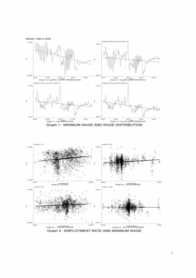
1

BRAZIL 1982 to 2000

Graph 1 - MINIMUM WAGE AND WAGE DISTRIBUTION

log

Graph 1.a - log REAL HOURLY MINIMUM WAGEyears

Jan 82 Jan 86 Jan 90 Jan 94 Jan 98

-.846282

.152526correlation with the real minimum wage: 0.78

log

Graph 1.b - log 25th WAGE PERCENTILEyears

Jan 82 Jan 86 Jan 90 Jan 94 Jan 98

-.325921

.372983

correlation with the real minimum wage: 0.74

log

Graph 1.c - log MEDIAN WAGEyears

Jan 82 Jan 86 Jan 90 Jan 94 Jan 98

.20116

1.0325

correlation with the real minimum wage: 0.73

log

Graph 1.d - log 75th WAGE PERCENTILEyears

Jan 82 Jan 86 Jan 90 Jan 94 Jan 98

.909363

1.78745

Graph 2 - EMPLOYMENT RATE AND MINIMUM WAGE

correlation: 0.181

rmw

Graph 2.a -LEVELSemployment rate

4.25317 5.66827

-.136498

-.018656

correlation: 0.054

rmw

Graph 2.b - 1st DIFFERENCEemployment rate

-.386635 .767518

-.03794

.031438

correlation: 0.211

rmw

Graph 2.c - 12TH DIFFERENCEemployment rate

-.629547 .543978

-.063908

.054828

correlation: -0.005

rmw

Graph 2.d - 1ST-12TH DIFFERENCEemployment rate

-.635726 .754579

-.041615

.047911

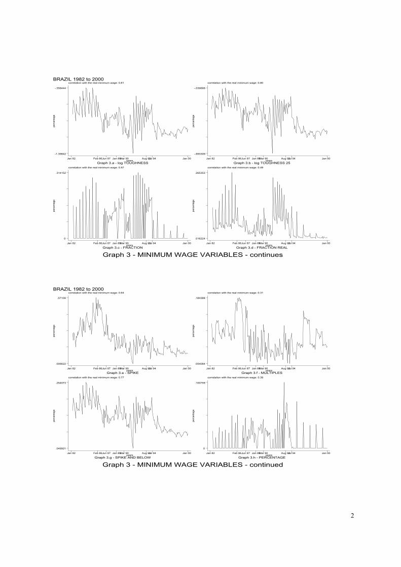
2

BRAZIL 1982 to 2000

Graph 3 - MINIMUM WAGE VARIABLES - continues

correlation with the real minimum wage: 0.81

perc

enta

ge

Graph 3.a - log TOUGHNESSyears

Jan 82 Feb 86Jun 87 Jan 89Mar 90 Aug 93Jul 94 Jan 00

-1.39842

-.556444

correlation with the real minimum wage: 0.80

perc

enta

ge

Graph 3.b - log TOUGHNESS 25years

Jan 82 Feb 86Jun 87 Jan 89Mar 90 Aug 93Jul 94 Jan 00

-.693309

-.039666

correlation with the real minimum wage: 0.57

perc

enta

ge

Graph 3.c - FRACTIONyears

Jan 82 Feb 86Jun 87 Jan 89Mar 90 Aug 93Jul 94 Jan 00

0

.314152

correlation with the real minimum wage: 0.49

perc

enta

ge

Graph 3.d - FRACTION REALyears

Jan 82 Feb 86Jun 87 Jan 89Mar 90 Aug 93Jul 94 Jan 00

.016224

.265353

BRAZIL 1982 to 2000

Graph 3 - MINIMUM WAGE VARIABLES - continued

correlation with the real minimum wage: 0.64

perc

enta

ge

Graph 3.e - SPIKEyears

Jan 82 Feb 86Jun 87 Jan 89Mar 90 Aug 93Jul 94 Jan 00

.006622

.07109

correlation with the real minimum wage: 0.31

perc

enta

ge

Graph 3.f - MULTIPLESyears

Jan 82 Feb 86Jun 87 Jan 89Mar 90 Aug 93Jul 94 Jan 00

.054084

.184388

correlation with the real minimum wage: 0.77

perc

enta

ge

Graph 3.g - SPIKE AND BELOWyears

Jan 82 Feb 86Jun 87 Jan 89Mar 90 Aug 93Jul 94 Jan 00

.049921

.254073

correlation with the real minimum wage: 0.39

perc

enta

ge

Graph 3.h - PERCENTAGEyears

Jan 82 Feb 86Jun 87 Jan 89Mar 90 Aug 93Jul 94 Jan 00

0

.100759

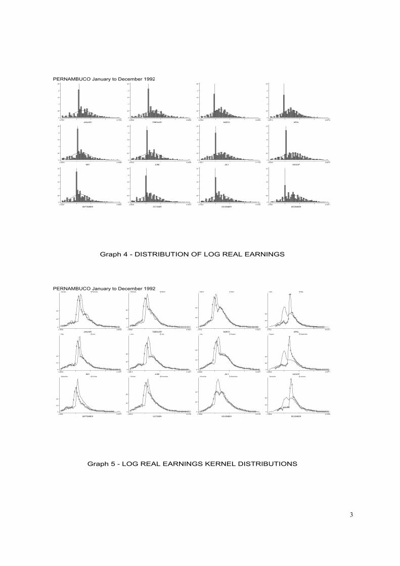
3

PERNAMBUCO January to December 1992

Graph 4 - DISTRIBUTION OF LOG REAL EARNINGS

.

JANUARY.

3.47401 8.772330

.05

.1

.15

.2

.25

.FEBRUARY

.3.24998 8.66608

0

.05

.1

.15

.2

.25

.

MARCH.

3.03395 9.654030

.05

.1

.15

.2

.25

.

APRIL.

2.84712 9.467190

.05

.1

.15

.2

.25

.

MAY.

3.53825 9.24998

0

.05

.1

.15

.2

.25

.

JUNE.

3.34378 9.20504

0

.05

.1

.15

.2

.25

.

JULY.

3.19011 9.11703

0

.05

.1

.15

.2

.25

.

AUGUST.

2.95325 8.88018

0

.05

.1

.15

.2

.25

.

SEPTEMBER.

3.62367 9.69852

0

.05

.1

.15

.2

.25

.

OCTOBER.

3.43699 9.24614

0

.05

.1

.15

.2

.25

.

NOVEMBER.

3.21553 9.24782

0

.05

.1

.15

.2

.25

.

DECEMBER.

2.87997 9.22811

0

.05

.1

.15

.2

.25

PERNAMBUCO January to December 1992

Graph 5 - LOG REAL EARNINGS KERNEL DISTRIBUTIONS

JANUARY.

January February

3.15095 8.865220

.03

.06

FEBRUARY.

February March

2.90387 9.784110

.03

.06

MARCH.

March April

2.7012 9.784110

.03

.06

APRIL.

April May

2.7012 9.613110

.03

.06

MAY.

May June

3.24846 9.183710

.03

.06

JUNE.

June July

3.06414 9.183710

.03

.06

JULY.

July August

2.80266 9.030770

.03

.06

AUGUST.

August September

2.80266 9.787710

.03

.06

SEPTEMBER.

September October

3.3355 9.787710

.03

.06

OCTOBER.

October November

3.09153 9.371820

.03

.06

NOVEMBER.

November December

2.70639 9.371820

.03

.06

DECEMBER.

December January

2.70639 9.376380

.03

.06

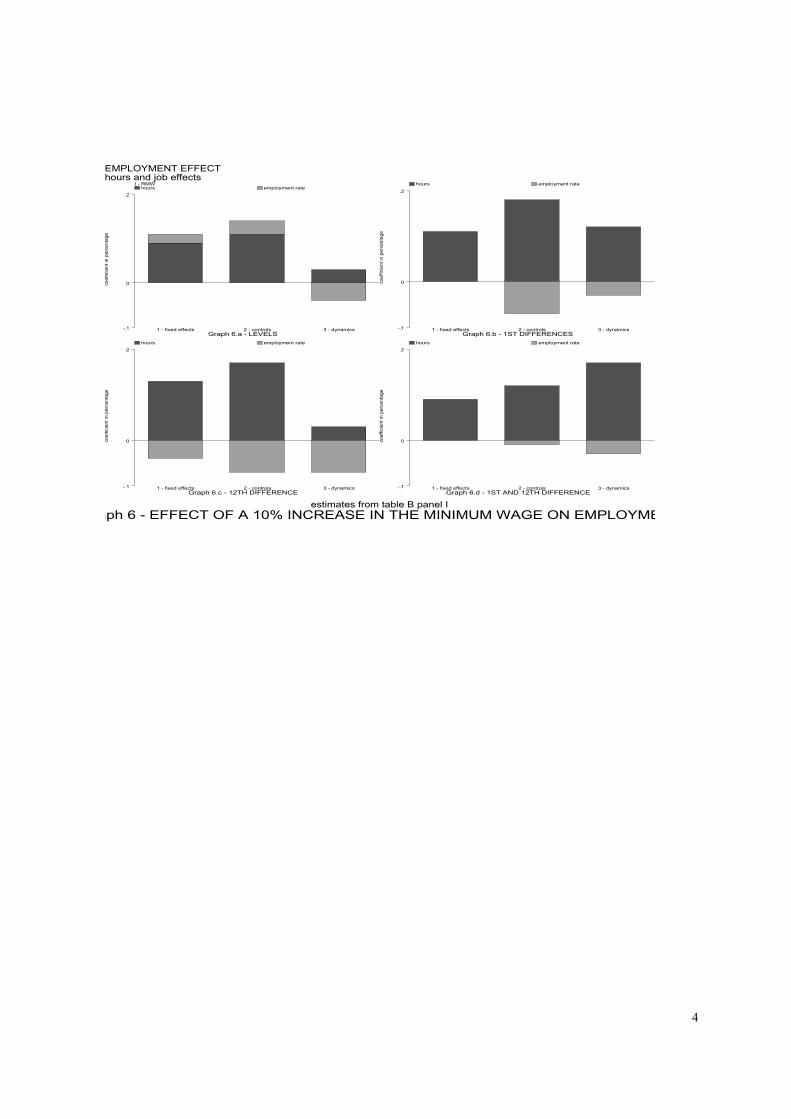
4

EMPLOYMENT EFFECThours and job effects

aph 6 - EFFECT OF A 10% INCREASE IN THE MINIMUM WAGE ON EMPLOYMEestimates from table B panel I

I - RMW

coef

ficie

nt in

per

cent

age

Graph 6.a - LEVELS-.1

0

.2 hours employment rate

1 - fixed effects 2 - controls 3 - dynamics

coef

ficie

nt in

per

cent

age

Graph 6.b - 1ST DIFFERENCES-.1

0

.2

hours employment rate

1 - fixed effects 2 - controls 3 - dynamics

coef

ficie

nt in

per

cent

age

Graph 6.c - 12TH DIFFERENCE-.1

0

.2 hours employment rate

1 - fixed effects 2 - controls 3 - dynamics

coef

ficie

nt in

per

cent

age

Graph 6.d - 1ST AND 12TH DIFFERENCE-.1

0

.2 hours employment rate

1 - fixed effects 2 - controls 3 - dynamics

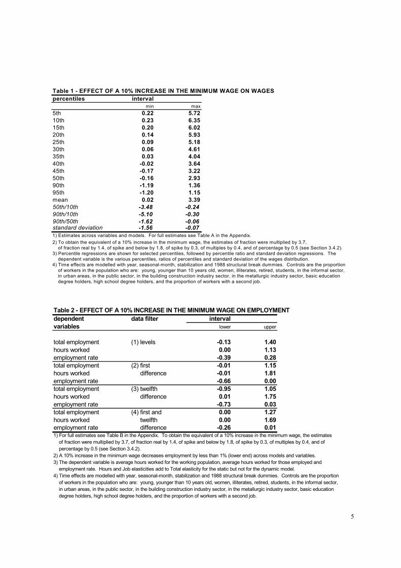
5

Table 1 - EFFECT OF A 10% INCREASE IN THE MINIMUM WAGE ON WAGESpercentiles interval

min max5th 0.22 5.7210th 0.23 6.3515th 0.20 6.0220th 0.14 5.9325th 0.09 5.1830th 0.06 4.6135th 0.03 4.0440th -0.02 3.6445th -0.17 3.2250th -0.16 2.9390th -1.19 1.3695th -1.20 1.15mean 0.02 3.3950th/10th -3.48 -0.2490th/10th -5.10 -0.3090th/50th -1.62 -0.06standard deviation -1.56 -0.071) Estimates across variables and models. For full estimates see Table A in the Appendix. 2) To obtain the equivalent of a 10% increase in the minimum wage, the estimates of fraction were multiplied by 3.7, of fraction real by 1.4, of spike and below by 1.8, of spike by 0.3, of multiples by 0.4, and of percentage by 0.5 (see Section 3.4.2).3) Percentile regressions are shown for selected percentiles, followed by percentile ratio and standard deviation regressions. The dependent variable is the various percentiles, ratios of percentiles and standard deviation of the wages distribution.4) Time effects are modelled with year, seasonal-month, stabilization and 1988 structural break dummies. Controls are the proportion of workers in the population who are: young, younger than 10 years old, women, illiterates, retired, students, in the informal sector, in urban areas, in the public sector, in the building construction industry sector, in the metallurgic industry sector, basic education degree holders, high school degree holders, and the proportion of workers with a second job.

Table 2 - EFFECT OF A 10% INCREASE IN THE MINIMUM WAGE ON EMPLOYMENTdependent data filter intervalvariables lower upper

total employment (1) levels -0.13 1.40hours worked 0.00 1.13employment rate -0.39 0.28total employment (2) first -0.01 1.15hours worked difference -0.01 1.81employment rate -0.66 0.00total employment (3) twelfth -0.95 1.05hours worked difference 0.01 1.75employment rate -0.73 0.03total employment (4) first and 0.00 1.27hours worked twelfth 0.00 1.69employment rate difference -0.26 0.011) For full estimates see Table B in the Appendix. To obtain the equivalent of a 10% increase in the minimum wage, the estimates of fraction were multiplied by 3.7, of fraction real by 1.4, of spike and below by 1.8, of spike by 0.3, of multiples by 0.4, and of percentage by 0.5 (see Section 3.4.2).2) A 10% increase in the minimum wage decreases employment by less than 1% (lower end) across models and variables.3) The dependent variable is average hours worked for the working population, average hours worked for those employed and employment rate. Hours and Job elasticities add to Total elasticity for the static but not for the dynamic model.4) Time effects are modelled with year, seasonal-month, stabilization and 1988 structural break dummies. Controls are the proportion of workers in the population who are: young, younger than 10 years old, women, illiterates, retired, students, in the informal sector, in urban areas, in the public sector, in the building construction industry sector, in the metallurgic industry sector, basic education degree holders, high school degree holders, and the proportion of workers with a second job.

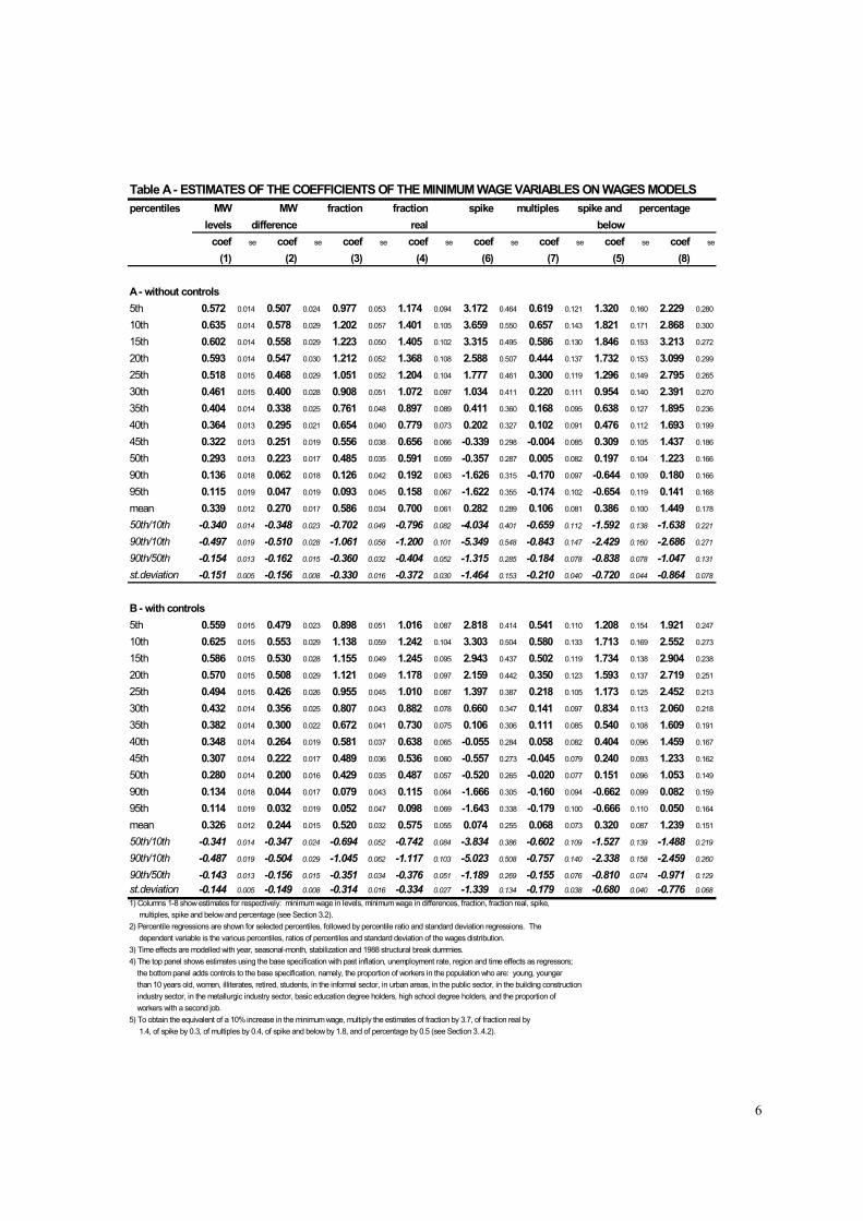
6

Table A - ESTIMATES OF THE COEFFICIENTS OF THE MINIMUM WAGE VARIABLES ON WAGES MODELS percentiles MW MW fraction fraction spike multiples spike and percentage

levels difference real belowcoef se coef se coef se coef se coef se coef se coef se coef se

(1) (2) (3) (4) (6) (7) (5) (8)

A - without controls5th 0.572 0.014 0.507 0.024 0.977 0.053 1.174 0.094 3.172 0.464 0.619 0.121 1.320 0.160 2.229 0.280

10th 0.635 0.014 0.578 0.029 1.202 0.057 1.401 0.105 3.659 0.550 0.657 0.143 1.821 0.171 2.868 0.300

15th 0.602 0.014 0.558 0.029 1.223 0.050 1.405 0.102 3.315 0.495 0.586 0.130 1.846 0.153 3.213 0.272

20th 0.593 0.014 0.547 0.030 1.212 0.052 1.368 0.108 2.588 0.507 0.444 0.137 1.732 0.153 3.099 0.299

25th 0.518 0.015 0.468 0.029 1.051 0.052 1.204 0.104 1.777 0.461 0.300 0.119 1.296 0.149 2.795 0.265

30th 0.461 0.015 0.400 0.028 0.908 0.051 1.072 0.097 1.034 0.411 0.220 0.111 0.954 0.140 2.391 0.270

35th 0.404 0.014 0.338 0.025 0.761 0.048 0.897 0.089 0.411 0.360 0.168 0.095 0.638 0.127 1.895 0.236

40th 0.364 0.013 0.295 0.021 0.654 0.040 0.779 0.073 0.202 0.327 0.102 0.091 0.476 0.112 1.693 0.199

45th 0.322 0.013 0.251 0.019 0.556 0.038 0.656 0.066 -0.339 0.298 -0.004 0.085 0.309 0.105 1.437 0.186

50th 0.293 0.013 0.223 0.017 0.485 0.035 0.591 0.059 -0.357 0.287 0.005 0.082 0.197 0.104 1.223 0.166

90th 0.136 0.018 0.062 0.018 0.126 0.042 0.192 0.063 -1.626 0.315 -0.170 0.097 -0.644 0.109 0.180 0.166

95th 0.115 0.019 0.047 0.019 0.093 0.045 0.158 0.067 -1.622 0.355 -0.174 0.102 -0.654 0.119 0.141 0.168

mean 0.339 0.012 0.270 0.017 0.586 0.034 0.700 0.061 0.282 0.289 0.106 0.081 0.386 0.100 1.449 0.178

50th/10th -0.340 0.014 -0.348 0.023 -0.702 0.049 -0.796 0.082 -4.034 0.401 -0.659 0.112 -1.592 0.138 -1.638 0.221

90th/10th -0.497 0.019 -0.510 0.028 -1.061 0.058 -1.200 0.101 -5.349 0.548 -0.843 0.147 -2.429 0.160 -2.686 0.271

90th/50th -0.154 0.013 -0.162 0.015 -0.360 0.032 -0.404 0.052 -1.315 0.285 -0.184 0.078 -0.838 0.078 -1.047 0.131

st.deviation -0.151 0.005 -0.156 0.008 -0.330 0.016 -0.372 0.030 -1.464 0.153 -0.210 0.040 -0.720 0.044 -0.864 0.078

B - with controls5th 0.559 0.015 0.479 0.023 0.898 0.051 1.016 0.087 2.818 0.414 0.541 0.110 1.208 0.154 1.921 0.247

10th 0.625 0.015 0.553 0.029 1.138 0.059 1.242 0.104 3.303 0.504 0.580 0.133 1.713 0.169 2.552 0.273

15th 0.586 0.015 0.530 0.028 1.155 0.049 1.245 0.095 2.943 0.437 0.502 0.119 1.734 0.138 2.904 0.238

20th 0.570 0.015 0.508 0.029 1.121 0.049 1.178 0.097 2.159 0.442 0.350 0.123 1.593 0.137 2.719 0.251

25th 0.494 0.015 0.426 0.026 0.955 0.045 1.010 0.087 1.397 0.387 0.218 0.105 1.173 0.125 2.452 0.213

30th 0.432 0.014 0.356 0.025 0.807 0.043 0.882 0.078 0.660 0.347 0.141 0.097 0.834 0.113 2.060 0.218

35th 0.382 0.014 0.300 0.022 0.672 0.041 0.730 0.075 0.106 0.306 0.111 0.085 0.540 0.108 1.609 0.191

40th 0.348 0.014 0.264 0.019 0.581 0.037 0.638 0.065 -0.055 0.284 0.058 0.082 0.404 0.096 1.459 0.167

45th 0.307 0.014 0.222 0.017 0.489 0.036 0.536 0.060 -0.557 0.273 -0.045 0.079 0.240 0.093 1.233 0.162

50th 0.280 0.014 0.200 0.016 0.429 0.035 0.487 0.057 -0.520 0.265 -0.020 0.077 0.151 0.096 1.053 0.149

90th 0.134 0.018 0.044 0.017 0.079 0.043 0.115 0.064 -1.666 0.305 -0.160 0.094 -0.662 0.099 0.082 0.159

95th 0.114 0.019 0.032 0.019 0.052 0.047 0.098 0.069 -1.643 0.338 -0.179 0.100 -0.666 0.110 0.050 0.164

mean 0.326 0.012 0.244 0.015 0.520 0.032 0.575 0.055 0.074 0.255 0.068 0.073 0.320 0.087 1.239 0.151

50th/10th -0.341 0.014 -0.347 0.024 -0.694 0.052 -0.742 0.084 -3.834 0.386 -0.602 0.109 -1.527 0.139 -1.488 0.219

90th/10th -0.487 0.019 -0.504 0.029 -1.045 0.062 -1.117 0.103 -5.023 0.508 -0.757 0.140 -2.338 0.158 -2.459 0.260

90th/50th -0.143 0.013 -0.156 0.015 -0.351 0.034 -0.376 0.051 -1.189 0.269 -0.155 0.076 -0.810 0.074 -0.971 0.129

st.deviation -0.144 0.005 -0.149 0.008 -0.314 0.016 -0.334 0.027 -1.339 0.134 -0.179 0.038 -0.680 0.040 -0.776 0.0681) Columns 1-8 show estimates for respectively: minimum wage in levels, minimum wage in differences, fraction, fraction real, spike, multiples, spike and below and percentage (see Section 3.2).2) Percentile regressions are shown for selected percentiles, followed by percentile ratio and standard deviation regressions. The dependent variable is the various percentiles, ratios of percentiles and standard deviation of the wages distribution.3) Time effects are modelled with year, seasonal-month, stabilization and 1988 structural break dummies.4) The top panel shows estimates using the base specification with past inflation, unemployment rate, region and time effects as regressors; the bottom panel adds controls to the base specification, namely, the proportion of workers in the population who are: young, younger than 10 years old, women, illiterates, retired, students, in the informal sector, in urban areas, in the public sector, in the building construction industry sector, in the metallurgic industry sector, basic education degree holders, high school degree holders, and the proportion of workers with a second job.5) To obtain the equivalent of a 10% increase in the minimum wage, multiply the estimates of fraction by 3.7, of fraction real by 1.4, of spike by 0.3, of multiples by 0.4, of spike and below by 1.8, and of percentage by 0.5 (see Section 3..4.2).

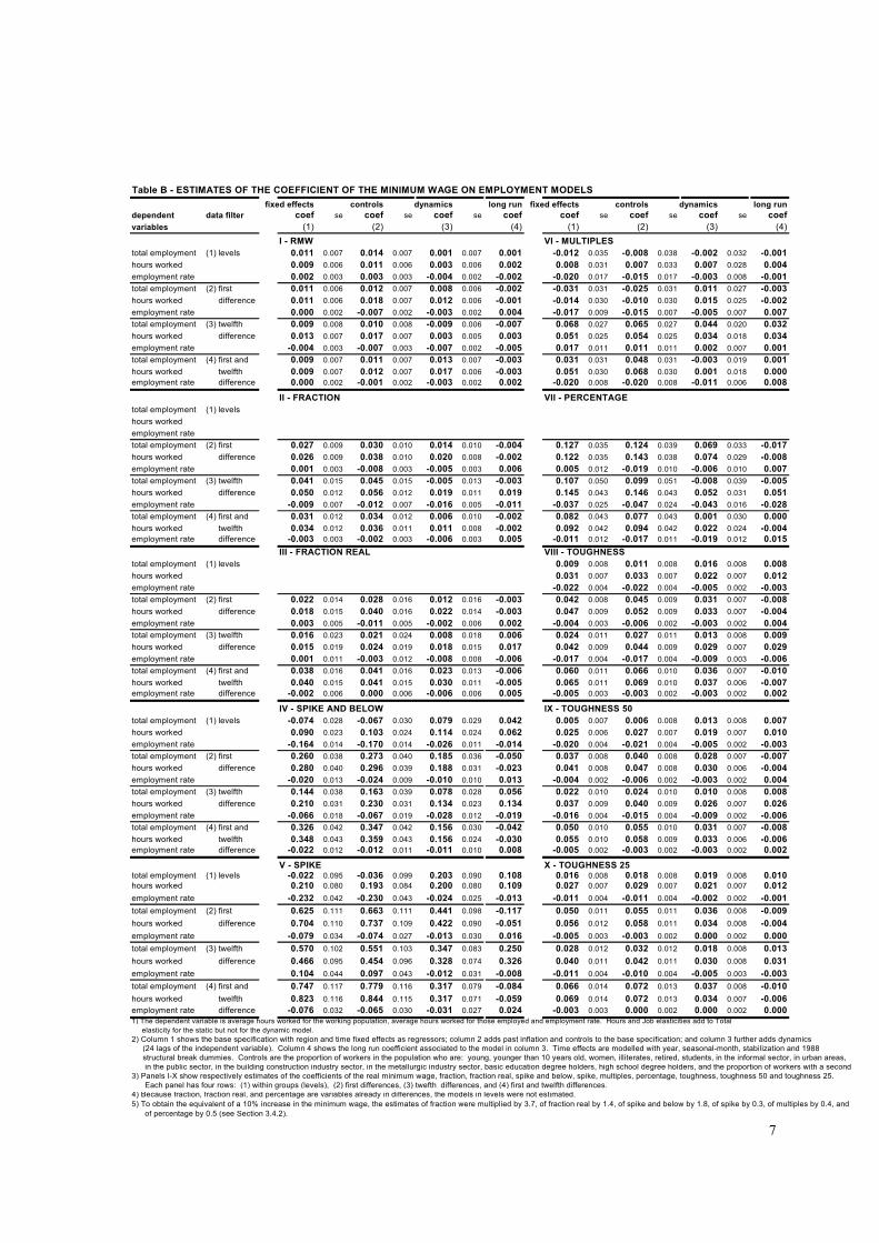
7

Table B - ESTIMATES OF THE COEFFICIENT OF THE MINIMUM WAGE ON EMPLOYMENT MODELSfixed effects controls dynamics long run fixed effects controls dynamics long run

dependent data filter coef se coef se coef se coef coef se coef se coef se coefvariables (1) (2) (3) (4) (1) (2) (3) (4)

I - RMW VI - MULTIPLEStotal employment (1) levels 0.011 0.007 0.014 0.007 0.001 0.007 0.001 -0.012 0.035 -0.008 0.038 -0.002 0.032 -0.001hours worked 0.009 0.006 0.011 0.006 0.003 0.006 0.002 0.008 0.031 0.007 0.033 0.007 0.028 0.004employment rate 0.002 0.003 0.003 0.003 -0.004 0.002 -0.002 -0.020 0.017 -0.015 0.017 -0.003 0.008 -0.001total employment (2) first 0.011 0.006 0.012 0.007 0.008 0.006 -0.002 -0.031 0.031 -0.025 0.031 0.011 0.027 -0.003hours worked difference 0.011 0.006 0.018 0.007 0.012 0.006 -0.001 -0.014 0.030 -0.010 0.030 0.015 0.025 -0.002employment rate 0.000 0.002 -0.007 0.002 -0.003 0.002 0.004 -0.017 0.009 -0.015 0.007 -0.005 0.007 0.007total employment (3) twelfth 0.009 0.008 0.010 0.008 -0.009 0.006 -0.007 0.068 0.027 0.065 0.027 0.044 0.020 0.032hours worked difference 0.013 0.007 0.017 0.007 0.003 0.005 0.003 0.051 0.025 0.054 0.025 0.034 0.018 0.034employment rate -0.004 0.003 -0.007 0.003 -0.007 0.002 -0.005 0.017 0.011 0.011 0.011 0.002 0.007 0.001total employment (4) first and 0.009 0.007 0.011 0.007 0.013 0.007 -0.003 0.031 0.031 0.048 0.031 -0.003 0.019 0.001hours worked twelfth 0.009 0.007 0.012 0.007 0.017 0.006 -0.003 0.051 0.030 0.068 0.030 0.001 0.018 0.000employment rate difference 0.000 0.002 -0.001 0.002 -0.003 0.002 0.002 -0.020 0.008 -0.020 0.008 -0.011 0.006 0.008

II - FRACTION VII - PERCENTAGEtotal employment (1) levelshours workedemployment ratetotal employment (2) first 0.027 0.009 0.030 0.010 0.014 0.010 -0.004 0.127 0.035 0.124 0.039 0.069 0.033 -0.017hours worked difference 0.026 0.009 0.038 0.010 0.020 0.008 -0.002 0.122 0.035 0.143 0.038 0.074 0.029 -0.008employment rate 0.001 0.003 -0.008 0.003 -0.005 0.003 0.006 0.005 0.012 -0.019 0.010 -0.006 0.010 0.007total employment (3) twelfth 0.041 0.015 0.045 0.015 -0.005 0.013 -0.003 0.107 0.050 0.099 0.051 -0.008 0.039 -0.005hours worked difference 0.050 0.012 0.056 0.012 0.019 0.011 0.019 0.145 0.043 0.146 0.043 0.052 0.031 0.051employment rate -0.009 0.007 -0.012 0.007 -0.016 0.005 -0.011 -0.037 0.025 -0.047 0.024 -0.043 0.016 -0.028total employment (4) first and 0.031 0.012 0.034 0.012 0.006 0.010 -0.002 0.082 0.043 0.077 0.043 0.001 0.030 0.000hours worked twelfth 0.034 0.012 0.036 0.011 0.011 0.008 -0.002 0.092 0.042 0.094 0.042 0.022 0.024 -0.004employment rate difference -0.003 0.003 -0.002 0.003 -0.006 0.003 0.005 -0.011 0.012 -0.017 0.011 -0.019 0.012 0.015

III - FRACTION REAL VIII - TOUGHNESStotal employment (1) levels 0.009 0.008 0.011 0.008 0.016 0.008 0.008hours worked 0.031 0.007 0.033 0.007 0.022 0.007 0.012employment rate -0.022 0.004 -0.022 0.004 -0.005 0.002 -0.003total employment (2) first 0.022 0.014 0.028 0.016 0.012 0.016 -0.003 0.042 0.008 0.045 0.009 0.031 0.007 -0.008hours worked difference 0.018 0.015 0.040 0.016 0.022 0.014 -0.003 0.047 0.009 0.052 0.009 0.033 0.007 -0.004employment rate 0.003 0.005 -0.011 0.005 -0.002 0.006 0.002 -0.004 0.003 -0.006 0.002 -0.003 0.002 0.004total employment (3) twelfth 0.016 0.023 0.021 0.024 0.008 0.018 0.006 0.024 0.011 0.027 0.011 0.013 0.008 0.009hours worked difference 0.015 0.019 0.024 0.019 0.018 0.015 0.017 0.042 0.009 0.044 0.009 0.029 0.007 0.029employment rate 0.001 0.011 -0.003 0.012 -0.008 0.008 -0.006 -0.017 0.004 -0.017 0.004 -0.009 0.003 -0.006total employment (4) first and 0.038 0.016 0.041 0.016 0.023 0.013 -0.006 0.060 0.011 0.066 0.010 0.036 0.007 -0.010hours worked twelfth 0.040 0.015 0.041 0.015 0.030 0.011 -0.005 0.065 0.011 0.069 0.010 0.037 0.006 -0.007employment rate difference -0.002 0.006 0.000 0.006 -0.006 0.006 0.005 -0.005 0.003 -0.003 0.002 -0.003 0.002 0.002

IV - SPIKE AND BELOW IX - TOUGHNESS 50total employment (1) levels -0.074 0.028 -0.067 0.030 0.079 0.029 0.042 0.005 0.007 0.006 0.008 0.013 0.008 0.007hours worked 0.090 0.023 0.103 0.024 0.114 0.024 0.062 0.025 0.006 0.027 0.007 0.019 0.007 0.010employment rate -0.164 0.014 -0.170 0.014 -0.026 0.011 -0.014 -0.020 0.004 -0.021 0.004 -0.005 0.002 -0.003total employment (2) first 0.260 0.038 0.273 0.040 0.185 0.036 -0.050 0.037 0.008 0.040 0.008 0.028 0.007 -0.007hours worked difference 0.280 0.040 0.296 0.039 0.188 0.031 -0.023 0.041 0.008 0.047 0.008 0.030 0.006 -0.004employment rate -0.020 0.013 -0.024 0.009 -0.010 0.010 0.013 -0.004 0.002 -0.006 0.002 -0.003 0.002 0.004total employment (3) twelfth 0.144 0.038 0.163 0.039 0.078 0.028 0.056 0.022 0.010 0.024 0.010 0.010 0.008 0.008hours worked difference 0.210 0.031 0.230 0.031 0.134 0.023 0.134 0.037 0.009 0.040 0.009 0.026 0.007 0.026employment rate -0.066 0.018 -0.067 0.019 -0.028 0.012 -0.019 -0.016 0.004 -0.015 0.004 -0.009 0.002 -0.006total employment (4) first and 0.326 0.042 0.347 0.042 0.156 0.030 -0.042 0.050 0.010 0.055 0.010 0.031 0.007 -0.008hours worked twelfth 0.348 0.043 0.359 0.043 0.156 0.024 -0.030 0.055 0.010 0.058 0.009 0.033 0.006 -0.006employment rate difference -0.022 0.012 -0.012 0.011 -0.011 0.010 0.008 -0.005 0.002 -0.003 0.002 -0.003 0.002 0.002

V - SPIKE X - TOUGHNESS 25total employment (1) levels -0.022 0.095 -0.036 0.099 0.203 0.090 0.108 0.016 0.008 0.018 0.008 0.019 0.008 0.010hours worked 0.210 0.080 0.193 0.084 0.200 0.080 0.109 0.027 0.007 0.029 0.007 0.021 0.007 0.012employment rate -0.232 0.042 -0.230 0.043 -0.024 0.025 -0.013 -0.011 0.004 -0.011 0.004 -0.002 0.002 -0.001total employment (2) first 0.625 0.111 0.663 0.111 0.441 0.098 -0.117 0.050 0.011 0.055 0.011 0.036 0.008 -0.009hours worked difference 0.704 0.110 0.737 0.109 0.422 0.090 -0.051 0.056 0.012 0.058 0.011 0.034 0.008 -0.004employment rate -0.079 0.034 -0.074 0.027 -0.013 0.030 0.016 -0.005 0.003 -0.003 0.002 0.000 0.002 0.000total employment (3) twelfth 0.570 0.102 0.551 0.103 0.347 0.083 0.250 0.028 0.012 0.032 0.012 0.018 0.008 0.013hours worked difference 0.466 0.095 0.454 0.096 0.328 0.074 0.326 0.040 0.011 0.042 0.011 0.030 0.008 0.031employment rate 0.104 0.044 0.097 0.043 -0.012 0.031 -0.008 -0.011 0.004 -0.010 0.004 -0.005 0.003 -0.003total employment (4) first and 0.747 0.117 0.779 0.116 0.317 0.079 -0.084 0.066 0.014 0.072 0.013 0.037 0.008 -0.010hours worked twelfth 0.823 0.116 0.844 0.115 0.317 0.071 -0.059 0.069 0.014 0.072 0.013 0.034 0.007 -0.006employment rate difference -0.076 0.032 -0.065 0.030 -0.031 0.027 0.024 -0.003 0.003 0.000 0.002 0.000 0.002 0.0001) The dependent variable is average hours worked for the working population, average hours worked for those employed and employment rate. Hours and Job elasticities add to Total elasticity for the static but not for the dynamic model.2) Column 1 shows the base specification with region and time fixed effects as regressors; column 2 adds past inflation and controls to the base specification; and column 3 further adds dynamics (24 lags of the independent variable). Column 4 shows the long run coefficient associated to the model in column 3. Time effects are modelled with year, seasonal-month, stabilization and 1988 structural break dummies. Controls are the proportion of workers in the population who are: young, younger than 10 years old, women, illiterates, retired, students, in the informal sector, in urban areas, in the public sector, in the building construction industry sector, in the metallurgic industry sector, basic education degree holders, high school degree holders, and the proportion of workers with a second3) Panels I-X show respectively estimates of the coefficients of the real minimum wage, fraction, fraction real, spike and below, spike, multiples, percentage, toughness, toughness 50 and toughness 25. Each panel has four rows: (1) within groups (levels), (2) first differences, (3) twefth differences, and (4) first and twelfth differences.4) Because fraction, fraction real, and percentage are variables already in differences, the models in levels were not estimated.5) To obtain the equivalent of a 10% increase in the minimum wage, the estimates of fraction were multiplied by 3.7, of fraction real by 1.4, of spike and below by 1.8, of spike by 0.3, of multiples by 0.4, and of percentage by 0.5 (see Section 3.4.2).

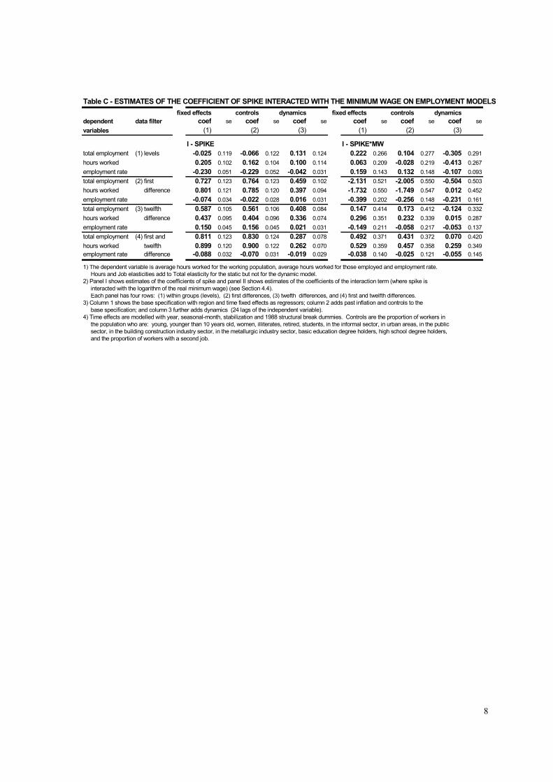
8

Table C - ESTIMATES OF THE COEFFICIENT OF SPIKE INTERACTED WITH THE MINIMUM WAGE ON EMPLOYMENT MODELSfixed effects controls dynamics fixed effects controls dynamics

dependent data filter coef se coef se coef se coef se coef se coef sevariables (1) (2) (3) (1) (2) (3)

I - SPIKE I - SPIKE*MWtotal employment (1) levels -0.025 0.119 -0.066 0.122 0.131 0.124 0.222 0.266 0.104 0.277 -0.305 0.291hours worked 0.205 0.102 0.162 0.104 0.100 0.114 0.063 0.209 -0.028 0.219 -0.413 0.267employment rate -0.230 0.051 -0.229 0.052 -0.042 0.031 0.159 0.143 0.132 0.148 -0.107 0.093total employment (2) first 0.727 0.123 0.764 0.123 0.459 0.102 -2.131 0.521 -2.005 0.550 -0.504 0.503hours worked difference 0.801 0.121 0.785 0.120 0.397 0.094 -1.732 0.550 -1.749 0.547 0.012 0.452employment rate -0.074 0.034 -0.022 0.028 0.016 0.031 -0.399 0.202 -0.256 0.148 -0.231 0.161total employment (3) twelfth 0.587 0.105 0.561 0.106 0.408 0.084 0.147 0.414 0.173 0.412 -0.124 0.332hours worked difference 0.437 0.095 0.404 0.096 0.336 0.074 0.296 0.351 0.232 0.339 0.015 0.287employment rate 0.150 0.045 0.156 0.045 0.021 0.031 -0.149 0.211 -0.058 0.217 -0.053 0.137total employment (4) first and 0.811 0.123 0.830 0.124 0.287 0.078 0.492 0.371 0.431 0.372 0.070 0.420hours worked twelfth 0.899 0.120 0.900 0.122 0.262 0.070 0.529 0.359 0.457 0.358 0.259 0.349employment rate difference -0.088 0.032 -0.070 0.031 -0.019 0.029 -0.038 0.140 -0.025 0.121 -0.055 0.145

1) The dependent variable is average hours worked for the working population, average hours worked for those employed and employment rate. Hours and Job elasticities add to Total elasticity for the static but not for the dynamic model.2) Panel I shows estimates of the coefficients of spike and panel II shows estimates of the coefficients of the interaction term (where spike is interacted with the logarithm of the real minimum wage) (see Section 4.4). Each panel has four rows: (1) within groups (levels), (2) first differences, (3) twefth differences, and (4) first and twelfth differences.3) Column 1 shows the base specification with region and time fixed effects as regressors; column 2 adds past inflation and controls to the base specification; and column 3 further adds dynamics (24 lags of the independent variable). 4) Time effects are modelled with year, seasonal-month, stabilization and 1988 structural break dummies. Controls are the proportion of workers in the population who are: young, younger than 10 years old, women, illiterates, retired, students, in the informal sector, in urban areas, in the public sector, in the building construction industry sector, in the metallurgic industry sector, basic education degree holders, high school degree holders, and the proportion of workers with a second job.