A Method for Gain over Temperature Measurements

Using Two “Hot” Noise Sources

Vince Rodriguez and Charles Osborne

MI Technologies: Suwanee, 30024 GA, USA vrodriguez@mitechnologies.com

Abstract—P Gain over Temperature (G/T) is an antenna

parameter of importance in both satellite communications and

radio-astronomy. Methods to measure G/T are discussed in the

literature [1-3]. These methodologies usually call for

measurements outdoors where the antenna under test (AUT) is

pointed to the “empty” sky to get a “cold” noise temperature

measurement; as required by the Y-factor measurement

approach [4]. In reference [5], Kolesnikoff et al. present a

method for measuring G/T in an anechoic chamber. In that

approach, the chamber has to be maintained at 290 kelvin to

achieve the “cold” reference temperature. In this paper, a new

method is presented intended for the characterization of lower

gain antennas, such as active elements of arrays. The new

method does not require a cold temperature reference; thus

alleviating the need for testing outside or maintaining a cold

reference temperature in a chamber. The new method uses two

separate “hot” sources. The two hot sources are created by using

two separate noise diode sources of known excess noise ratios

(ENR) or by one source and a known attenuation. The key is that

the sources differ by a known amount. This paper builds upon

the presented information in [2] providing more measured data

using the recommended procedure.

I. INTRODUCTION

It follows Maxwell’s Equations that accelerating charges radiate. Since atoms contain charges, and vibrate proportionally to the temperature, materials radiate proportionally to the temperature. This radiation is evenly distributed across the frequency band to 300GHz. The power of this radiation in watts is given by the following equation:

𝑃𝑛 = 𝑘𝑇𝑛𝐵 (1)

where Pn is the thermal noise power in watts, k is Boltzmann’s constant (1.38·10

-23 J/K/Hz), Tn is the temperature in Kelvin

and B is the bandwidth in Hz. It is common to refer to the noise temperature of a system. This noise temperature is not the actual ambient temperature in K, but the temperature at which a resistor heated to that given temperature will radiate that equivalent noise power.

II. THEORETICAL BACKGROUND

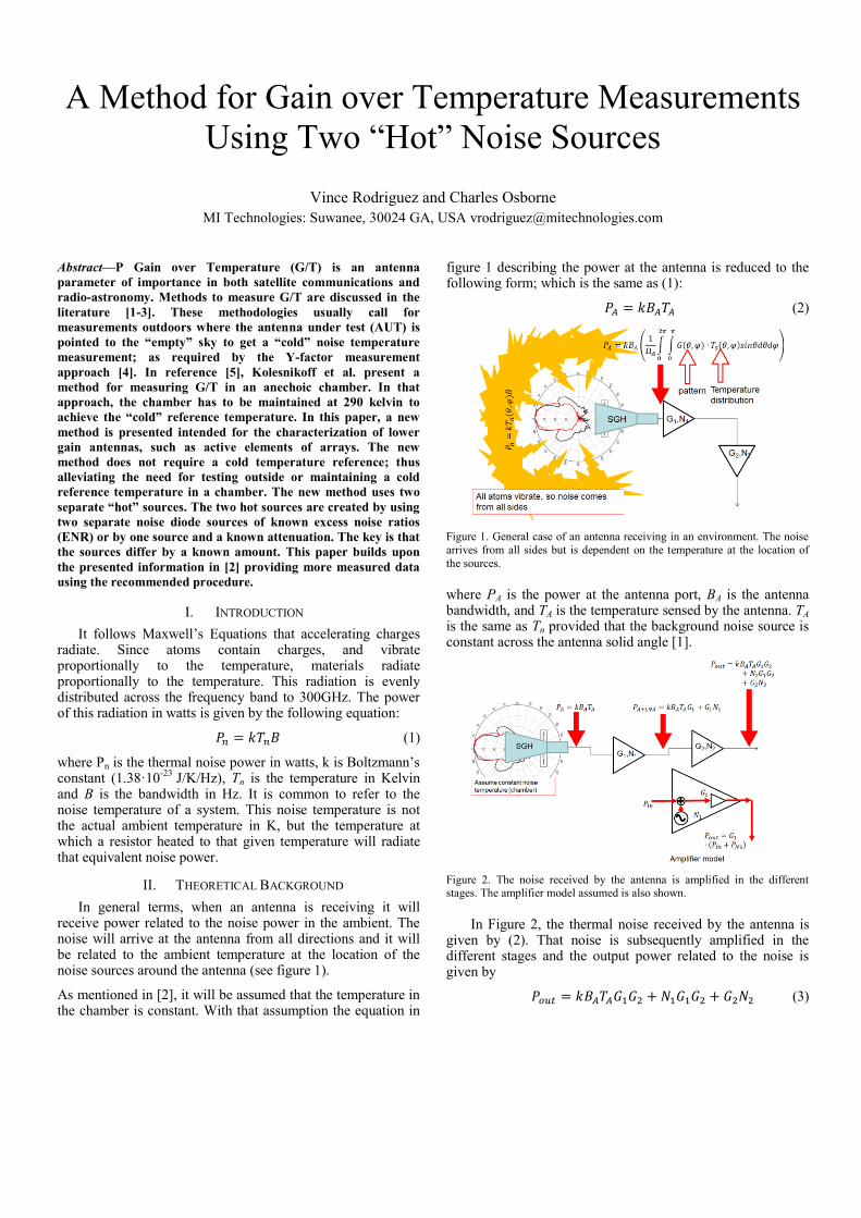
In general terms, when an antenna is receiving it will receive power related to the noise power in the ambient. The noise will arrive at the antenna from all directions and it will be related to the ambient temperature at the location of the noise sources around the antenna (see figure 1).

As mentioned in [2], it will be assumed that the temperature in the chamber is constant. With that assumption the equation in

figure 1 describing the power at the antenna is reduced to the following form; which is the same as (1):

𝑃𝐴 = 𝑘𝐵𝐴𝑇𝐴 (2)

Figure 1. General case of an antenna receiving in an environment. The noise

arrives from all sides but is dependent on the temperature at the location of

the sources.

where PA is the power at the antenna port, BA is the antenna bandwidth, and TA is the temperature sensed by the antenna. TA is the same as Tn provided that the background noise source is constant across the antenna solid angle [1].

Figure 2. The noise received by the antenna is amplified in the different stages. The amplifier model assumed is also shown.

In Figure 2, the thermal noise received by the antenna is

given by (2). That noise is subsequently amplified in the different stages and the output power related to the noise is given by

𝑃𝑜𝑢𝑡 = 𝑘𝐵𝐴𝑇𝐴𝐺1𝐺2 + 𝑁1𝐺1𝐺2 + 𝐺2𝑁2 (3)

Now, the system noise, the noise introduces in the amplifier stages is given by the noise temperature of the stages, hence

𝑃𝑆𝑦𝑠𝑡𝑒𝑚 = 𝑘𝑇𝑆𝑦𝑠𝐵 (4)

Using (4) on the noise contributions from the system is

𝑇𝑆𝑦𝑠 = +𝑁1𝐺1𝐺2

𝑘𝐵+

𝑁2𝐺2

𝑘𝐵

𝐺1

𝐺1 (5)

From (5) the noise temperature for each stage is given by

𝑇𝑆𝑦𝑠 = 𝑇1 +𝑇2

𝐺1 (6)

From this we arrive the equation for gain over temperature; where gain G is the gain of the antenna in the system and the gains of the amplifiers (or the losses) are accounted in the noise temperature of each stage.

𝐺

𝑇=

𝐺

𝑇𝐴+𝑇𝑆𝑦𝑠 (7)

As shown in [2], the equation can be made more general by adding the noise contribution due to antenna physical temperature and its losses. However, for the methodology, since two “hot” sources are used, we can ignore the noise contribution due to the antenna temperature.

The approach to measure the G/T follows the Y-factor

measurement described in [2 and 4]. In reference [6], the

noise figure is the signal to noise ratio into the stage divided

by the signal to noise ratio at the output of the stage

𝐹 =(𝑆𝑖𝑛𝑁𝑖𝑛

)

(𝑆𝑜𝑢𝑡𝑁𝑜𝑢𝑡

)=

𝑆𝑁𝑅𝑖𝑛

𝑆𝑁𝑅𝑜𝑢𝑡 (8)

Reference [6] shows that the noise figure F can be written in terms of the noise temperature of the device Te and the standard temperature To of 290K.

𝐹 =𝑇𝑒

𝑇0+ 1 (9)

Y factor measurements require the use of a noise source with a pre-calibrated ENR, the ENR s defined as

𝐸𝑁𝑅 =(𝑇𝑆

𝑂𝑁−𝑇𝑆𝑂𝐹𝐹)

𝑇0 (10)

where TSOFF

is the physical temperature of the device in K. The ENR is used to compute the noise temperature of the noise source at a given frequency. The Y factor is a ratio of two different noise levels. Traditionally the procedure has been to turn the noise source on and then off and use those noise levels to get the Y factor. Hence the Y factor is given by

𝑌 =𝑁𝑂𝑁

𝑁𝑂𝐹𝐹=

𝑇𝑂𝑁

𝑇𝑂𝐹𝐹 (11)

The procedure calls for a calibration in which the Y factor of the receiver is measured [4]. From this calibration the noise temperature of the receiver can be calculated.

𝑇𝑟𝑥 =(𝑇𝑠

𝑂𝑁−𝑌𝑟𝑥𝑇𝑆𝑂𝐹𝐹)

(𝑌𝑟𝑥−1) (12)

where the subscript rx indicates the receiver. The measurement can be done in the device under test (DUT) and then (6) can be rewritten as

𝑇𝑆𝑦𝑠 = 𝑇𝐷𝑈𝑇 +𝑇𝑟𝑥

𝐺𝐷𝑈𝑇 (13)

Hence the DUT noise temperature can be obtained.

Using the derived GDUT and TDUT the gain over temperature can be computed. The procedure is similar for antennas. If the antenna can be removed from the active network the standard procedure in [4] can be follow for the amplifiers.

In this paper we look at a methodology that can be used for antennas that have integrated active components or for antenna array elements. The method is intended to provide a figure for the noise of an integrated amplifier into the antenna. The noise sensed by the antenna when deployed will be different than the noise in the anechoic chamber. The critical factor utilizing this G/T measurement approach is that it allows a system level measurement of performance to be performed aggregating antenna gain, noise figure, distributed losses, and matching effects in situ. In practice, most antenna installations will not see ambient thermal radiation in all directions leading to slightly better performance than indicated. But by using T-cold of at least 3000 Kelvin in this two-noise-source approach, that measurement difference can be minimized.

III. PROCEDURE FOR ANTENNAS

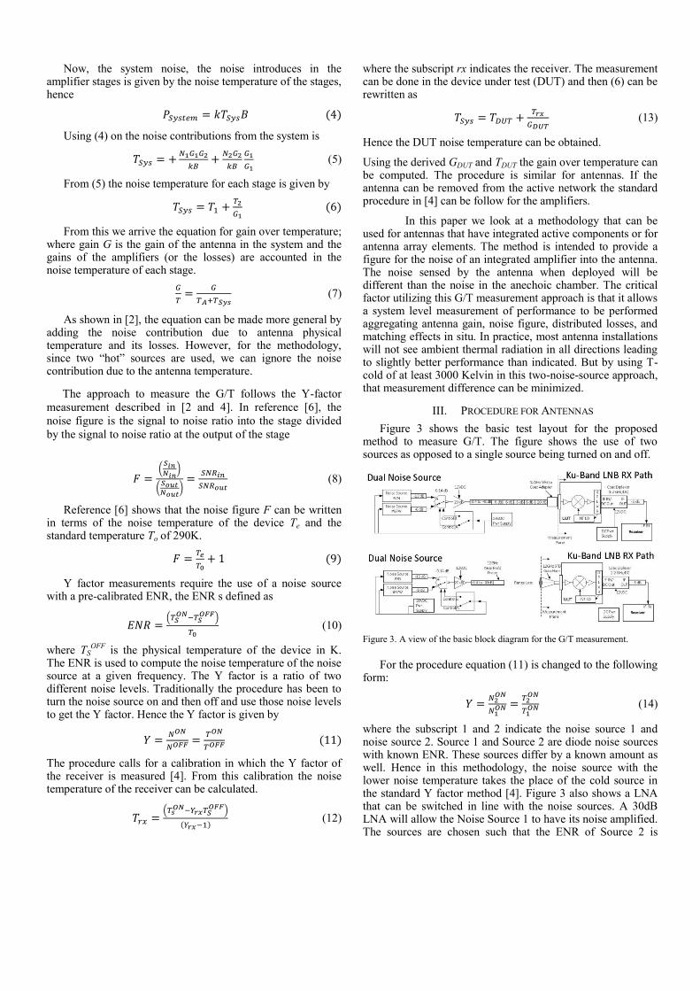
Figure 3 shows the basic test layout for the proposed method to measure G/T. The figure shows the use of two sources as opposed to a single source being turned on and off.

Figure 3. A view of the basic block diagram for the G/T measurement.

For the procedure equation (11) is changed to the following

form:

𝑌 =𝑁2𝑂𝑁

𝑁1𝑂𝑁 =

𝑇2𝑂𝑁

𝑇1𝑂𝑁 (14)

where the subscript 1 and 2 indicate the noise source 1 and noise source 2. Source 1 and Source 2 are diode noise sources with known ENR. These sources differ by a known amount as well. Hence in this methodology, the noise source with the lower noise temperature takes the place of the cold source in the standard Y factor method [4]. Figure 3 also shows a LNA that can be switched in line with the noise sources. A 30dB LNA will allow the Noise Source 1 to have its noise amplified. The sources are chosen such that the ENR of Source 2 is

higher than Source 1. These high noise temperatures can be used to take into account the losses between the output of the LNA and the input of the DUT to allow sufficient signal to noise to measure the Y factor. The use of these two “hot” sources minimizes the effects of ambient temperature changes

as long as both are greater than 10 dB above the ambient thermal noise. The noise introduced by the components from the ambient temperature, is negligible when compared to the equivalent noise temperatures of the sources.

Figure 4. Line diagram.

Referring to Figure 4, at point “A” Source 1 is 1,000 Kelvin and Source 2 is 10,000 Kelvin are alternately switched into the system. As this noise passes through the LNA the noise is increased by the LNA gain plus its own noise contribution (5.5dB noise figure = 740 Kelvin). If the amplifier has a gain of 30dB, the noise now becomes 1,740,000 Kelvin for Source 1, and 10,740,000 Kelvin equivalent for Source 2, at point “B”. If the sum of all the fixed and variable losses between “B” and “E” is 30dB, the noise power input to the DUT at “E” is reduced by a factor of 1,000. This leaves Source 1 = 1,740 Kelvin at the input of the DUT. However, the attenuators and cables add their own thermal noise, but Source 1 dominates the noise. Source 2 is 10 dB more noise, also dominating the noise contribution of the attenuators and cables.

T-Hot at “E” is 1,740,000/1,000 = 1,740 Kelvin. If compared to ambient T-Cold this leaves only an ENR = 10 LOG ( 1740 / 290 ) =7.8dB a usable amount of noise to make the measurement. In an anechoic chamber, the absorber completely surrounds the receive antenna’s field of view. Increasing the gain of the antenna causes it to see a smaller area of absorber, making received noise power constant unless something of higher physical temperature is in the antenna field of view. However the noise source when turned on illuminates the room with 10,000 Kelvin noise. The absorber reradiates only a small portion of that power. Only the portion of this noise collected by the receive antenna affects the output noise power. This loss between feed and DUT is what must be characterized.

Another noise contributor is the receive power measuring system itself. If the DUT gain is low, the receive system’s own noise power will affect the noise power reading during T-Hot to T-cold measuring. If the receive noise power measuring system has a 24dB noise figure its own noise floor is -15 dBm/Hz. Mixer losses further degrade this to -136dBm/Hz for an equivalent noise figure at point “H” of approximately [-174 – (-136)]= 38dB noise figure. Post DUT gain of 30dB divides this down so that the effect at “G” is only 6,309/1000 = 6.3 Kelvin added noise. This adds less than 0.1dB to the post DUT LNA’s noise figure of 5dB, resulting in 5.1dB noise figure at “G” looking toward the measurement system receiver. System losses of 5dB in cable and switch loss add directly to the noise figure. So at “F” looking toward the measurement system, the noise figure becomes 5.1+5dB = 10.1dB. This is 2700 Kelvin equivalent. If DUT gain is below 20dB, the receive system noise begins to contribute to an error term which the DUT gain has to overcome. At 10dB gain, the error term becomes

exponentially larger. At 30dB DUT gain, the term becomes small (See Figure 9). Working between the unknowns caused by system losses and noise figures increasing with frequency, knowing the DUT gain a priori becomes important to stay above the noise floor, and below any gain compression effects.

A. Deriving Losses

In this part of the measurement, the normal range configuration is calibrated by using a power meter after the source switch at test point “B”. The common port of the switch goes to the feed open ended waveguide (OEW) probe. The noise source is connected to the other port. Power is measured at all available points over the frequency range of interest. A low noise amplifier of known gain and noise figure is also used to bridge the DUT to OEWG probe input switch. This allows the known noise figure of the LNA to dominate the link budget equations and overcome any second stage contribution of noise which may show up in the DUT noise figure. It can be used similar to a standard gain horn as a way of comparing DUT gain and noise figure when used in one of the calibration signal paths. Adding a 3dB attenuator ahead of the LNA should add 3dB to the noise figure. This is another good cross check of system dynamic range. Working through the system by substitution using the source and attenuators the loss contribution over frequency of each subsystem part can be derived and recorded for future use.

B. Linearity

Noise Figure can’t be measured accurately if any of the components are being driven into compression when the noise source is turned ON. The resulting measurements will indicate noise figure readings lower than if no compression was present. A noise source is a broadband signal which can have more total power than might be assumed in a narrowband comparison in the receiver or spectrum analyzer. The total power in the receiver is measured. Then a signal generator output is increased until the receiver approximately matches the power reading for the noise source. The signal generator level is increased by 10 dB and measured to check for compression. If more than 0.05 dB compression is present, the operating point should be changed by changing attenuation/gain and feed probe spacing, until this measurement runs with no compression. The LNA’s output can be attenuated if mixer compression is occurring. But minimal attenuation should be used to insure good signal to noise ratios are achieved with no effect on the noise figure. The preliminary measurements shown in the present paper are centered in finding this no-compression region.

C. Temperature

It is important to have a stable ambient temperature to reduce amplifier gain changes during the measurements. Most noise sources do warm up slightly due to current in the diode and associated circuitry. At least 30 minutes is recommended for the sources to stabilize. This is usually more important for the wired calibration, since room ambient dominates when the

two feeds are far enough apart to make the noise source noise power not be seen above the room noise. Using a switch with at least 40 dB of isolation, both noise sources can be left on continuously eliminating effects from warm up. As previously mentioned, if both the noise source T-Hot Source 1 and T-Hot Source 2 are insufficient to maintain good signal to noise in this measurement, the gain of the LNA after the switch (point A to point B) must be used as a power amplifier for the noise source. A 40 dB gain LNA for example will increase a 15dB ENR (10,000 Kelvin) noise source to become a 55dB (100 Million Kelvin equivalent) ENR source. If followed by 10 dB of system losses this becomes 10 million Kelvin or 45dB ENR equivalent. The goal is to balance system gains and losses to not be in compression, while maximizing signal to noise and measurement accuracy, as the preliminary measurements will demonstrate.

D. Accuracy

Measurement accuracy is proportional to attention to detail in noise figure measurements. Each component between noise source and LNA normally has specifications with associated ± errors. Without refining these numbers at spot frequencies, the worst case numbers quickly exceed the measured noise figure. The noise source is typically ±0.7dB specified error compared to the label value. It can be much better if temperature is held constant and accumulated small losses can be compensated by comparison to a known noise figure LNA measured in place of the DUT. Seldom do all errors fall on the same side of worst case. It is much more common to see a more random distribution of errors leading to RMS being commonly used to derive the expected error function. Using the variable attenuators it is possible to cross check some system measurements multiple ways to be sure operation is within the linear range. The cover of [4] shows the plot in Figure 5.

Figure 5. Plot from the cover of reference [4] showing uncertainty versus the

DUT characteristics. (courtesy of Keysight)

This shows that measurement uncertainty increases for low

gain LNAs and low noise figures (under 2 dB). That’s why a

known noise figure and gain LNA may be necessary in the

test system itself to insure calibration accuracy prior to

placing the DUT/LNA combination in line. Return loss

interactions add additional uncertainty which can change with

small changes in connector or cable lengths.

IV. NUMERICAL RESULTS FOR SPACE LOSS

One of the keys to this procedure is to account for the

losses. The loss between the OEWG probe and the AUT is

critical since the reference plane for the measurement of the

AUT is the aperture of the AUT. For the preliminary results a

standard gain horn (SGH) is being used as the AUT. The

OEWG and SGH are modeled at a separation of 5λ and 10λ.

Where λ is the free space wavelength at 10.2GHz, thus, the

separation is 12.696cm at 5λ and 29.391cm at 10λ. Even at

the shorter separation of 5λ as the OEWG radiates it covers

the entire aperture of the SGH. This can be seen in Figure 6.

Figure 6. Field distribution of the OEWG probe radiating at a distance of 5λ from the aperture of the SGH.

The coupling between the OEWG and the SGH is shown in

Figure 7. This coupling is basically the loss between the

OEWG port and the SGH port.

Figure 7. The coupling between the OEWG and the SGH at two distances. The OEWG is radiating while the SGH is receiving. The numerical model

geometry is shown on the upper right corner of the plot.

The coupling at 12.17GHz is -21.50dB for the 5λ separation

between the aperture of the OEWG and the aperture of the

SGH. While for a separation of 10λ the coupling is computed

as -23.92dB. However, a more precise data point is to look not

at the power at Port 2 (the AUT port) versus Port 1, (the

OEWG port), but to integrate over the aperture of the AUT to

get an estimate of the incident power at the AUT. When doing

this simulation, a priori knowledge of the AUT is required.

V. PRELIMINARY MEASUREMENTS

In this section, preliminary measurements are presented. At the time of submitting the present paper, the measurements performed are related to achieving the required linearity in the

system described in Part B of Section IV. For these preliminary measurements, an anechoic range was not available so a bench-top set up was used for proof of concept. Figure 8 shows the test set up.

Figure 8. Test set up for preliminary measurements. The test area was surrounded by anechoic material during the radiated tests.

As it can be seen in Figure 8, the preliminary test setup is not

ideal. Future work has to be done to repeat some of the

measurements in a more typical range.

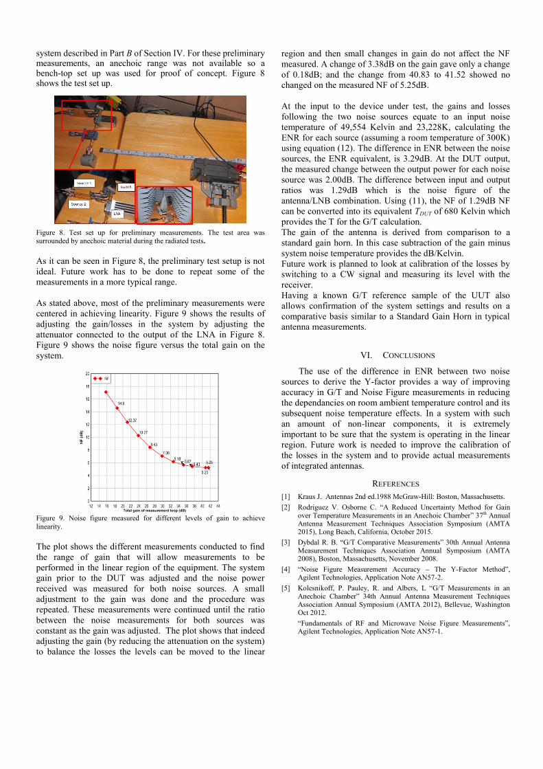
As stated above, most of the preliminary measurements were

centered in achieving linearity. Figure 9 shows the results of

adjusting the gain/losses in the system by adjusting the

attenuator connected to the output of the LNA in Figure 8.

Figure 9 shows the noise figure versus the total gain on the

system.

Figure 9. Noise figure measured for different levels of gain to achieve

linearity.

The plot shows the different measurements conducted to find

the range of gain that will allow measurements to be

performed in the linear region of the equipment. The system

gain prior to the DUT was adjusted and the noise power

received was measured for both noise sources. A small

adjustment to the gain was done and the procedure was

repeated. These measurements were continued until the ratio

between the noise measurements for both sources was

constant as the gain was adjusted. The plot shows that indeed

adjusting the gain (by reducing the attenuation on the system)

to balance the losses the levels can be moved to the linear

region and then small changes in gain do not affect the NF

measured. A change of 3.38dB on the gain gave only a change

of 0.18dB; and the change from 40.83 to 41.52 showed no

changed on the measured NF of 5.25dB.

At the input to the device under test, the gains and losses

following the two noise sources equate to an input noise

temperature of 49,554 Kelvin and 23,228K, calculating the

ENR for each source (assuming a room temperature of 300K)

using equation (12). The difference in ENR between the noise

sources, the ENR equivalent, is 3.29dB. At the DUT output,

the measured change between the output power for each noise

source was 2.00dB. The difference between input and output

ratios was 1.29dB which is the noise figure of the

antenna/LNB combination. Using (11), the NF of 1.29dB NF

can be converted into its equivalent TDUT of 680 Kelvin which

provides the T for the G/T calculation.

The gain of the antenna is derived from comparison to a

standard gain horn. In this case subtraction of the gain minus

system noise temperature provides the dB/Kelvin.

Future work is planned to look at calibration of the losses by

switching to a CW signal and measuring its level with the

receiver.

Having a known G/T reference sample of the UUT also

allows confirmation of the system settings and results on a

comparative basis similar to a Standard Gain Horn in typical

antenna measurements.

VI. CONCLUSIONS

The use of the difference in ENR between two noise

sources to derive the Y-factor provides a way of improving

accuracy in G/T and Noise Figure measurements in reducing

the dependancies on room ambient temperature control and its

subsequent noise temperature effects. In a system with such

an amount of non-linear components, it is extremely

important to be sure that the system is operating in the linear

region. Future work is needed to improve the calibration of

the losses in the system and to provide actual measurements

of integrated antennas.

REFERENCES

[1] Kraus J. Antennas 2nd ed.1988 McGraw-Hill: Boston, Massachusetts.

[2] Rodriguez V. Osborne C. “A Reduced Uncertainty Method for Gain over Temperature Measurements in an Anechoic Chamber” 37th Annual Antenna Measurement Techniques Association Symposium (AMTA 2015), Long Beach, California, October 2015.

[3] Dybdal R. B. “G/T Comparative Measurements” 30th Annual Antenna Measurement Techniques Association Annual Symposium (AMTA 2008), Boston, Massachusetts, November 2008.

[4] “Noise Figure Measurement Accuracy – The Y-Factor Method”, Agilent Technologies, Application Note AN57-2.

[5] Kolesnikoff, P. Pauley, R. and Albers, L “G/T Measurements in an Anechoic Chamber” 34th Annual Antenna Measurement Techniques Association Annual Symposium (AMTA 2012), Bellevue, Washington Oct 2012.

“Fundamentals of RF and Microwave Noise Figure Measurements”, Agilent Technologies, Application Note AN57-1.