a methodology for analyzing emission control strategies

Cornput. dt 0~s Res.. Vol. 3, pp. M-207. Perpmon Press, I!% Printed in Great Britain

A METHODOLOGY FOR ANALYZING EMISSION CONTROL STRATEGIES

D. WARNER NORTH* and M. W. ME~OFER~

scope and -This paper presents an analysis of alternative methods for con~o~mg sulfur oxide emissions from coal fired electric generating plants. The analysis was carried out in support of a study by a committee of the National Academy of Sciences.

An extensive discussion of the analysis and the information on which it is based is included in the National Academy report [ 11. The presentation given here is intended as a summary for the reader interested primarily in the methodolo~ employed in the analysis.

Abstract-Alternative strategies for controlling sulfur oxide emissions from representative coal fired electric power plants are evaiuated both in terms of their economic and environmental impacts. A framework is provided for converting environmental impacts to human health, ecological, aesthetic, and material damage costs borne by society. A imprison of these costs to the costs of ~Rution control provides the basis for choice among available strategies. Existing uncertainties in health effects and SO,, atmospheric transport and conversion are explicitly represented. These uncertainties are shown to be crucial to the decision among control strategies. Computations show the resolution of these uncertainties to be worth hundreds of millions of dollars per year.

1. INTRODUCTION

Applications of cost-benefit analysis to decisions relating to the control of air and water pollutant emissions have been relatively rare. Traditional practice in the U.S. has been to establish standards for emissions and ambient levels of hazardous substances in the air and water. The standards usually reflect judgment that there is a threshold for the onset of health and other adverse effects, and that if the ambient level of the pollutant can be brought below the levels established by the standard, the adverse effects will be eliminated.

Unfortunately, this viewpoint often proves simplistic in practice. Adverse effects on health and property may occur at very low condensations, and a statistical basis for assessing the magnitude of the damages occurring at low concentrations may be difficult and costly, perhaps impossible, to establish. The control strategies needed to reduce emissions may impose substantial added costs on goods and services desired by the public. Rather than have a sharp standard d~erentiating allowable from forbidden emissions levels, it would be desirable to carry out a cost-benefit analysis in which the marginal cost of removing a unit quantity of emissions is compared to the marginal benefit of doing so. The decision on emission control would then be made on an economic basis: If the benefit from emissions reduction exceeds the cost imposed by the control strategy, then the control should be applied. Economists have noted that a tax on emissions would be one way to institutionalize this means of decision-making[21, but this has rarely been carried out in practice. A major difficulty is that the benefits from emission control are difficult to measure and are typically very uncertain.

Sulfur oxide emissions from power plants provide an excellent illustration of the problems encountered in a standards approach. Whereas there is an ambient standard for sulfur dioxide, no standard has been established for sulfate particles that are formed by atmospheric oxidation of the sulfur dioxide. Laboratory tests on animals and epidemiological studies such as those carried out by CHESS [3] indicate that sulfates may have substantial adverse effects on health even at levels approaching natural background ambient concentrations. Finally, control of sulfur oxide emissions is expensive: Presently available flue gas desulfurization technologies such as lime scrubbing can remove 90% of the sulfur oxides, but at a cost on the order of a 20% increase in the wholesale price of electricity. Is this added cost to the consumers of electricity justified by the benefits of the emissions reduction?

*D. Warner North received his Ph,D in Operations Research from Stanford University in 1970, and he is presently the Assistant Director of the Decision Analysis Group at the Stanford Research Institute. He has published a number of papers on decision analysis and its application to problems’ in the pubtic sector.

tMiley W. Merkhofer received his Ph.D. in Engineering Economic Systems from Stanford University in 1975. He is presently employed by the Stanford Research Institute as a decision analyst and periodically teaches management science courses for the University Extension, University of California at Berkeley.

185

186 D. WARNER NORTH and M. W. MERKHOFER

In the fall of 1974 the authors were asked to carry out an analysis of alternative strategies for sulfur oxide control in support of a National Academy of Sciences study on air quality and stationary source emission control. It was our objective to carry out an application of the cost-benefit approach, although we had only a few months time and a very limited base of i~ormation on which to build our analysis. The goal of our effort was to summarize the information available as a basis for the decision on which the Academy Committee had been asked to make recommendations: Should presently available control technologies be deployed in order to reduce sulfur oxide emissions from coal burning power plants? Where i~ormation was limited and the consequences of emission control uncertain, our goal was to characterize the ~ce~ainty and to determine the value of resolving this uncertainty in the context of national decisions on sulfur oxide control.

The discussion presented here is a summary of the analysis carried out for the National Academy and is intended for the reader interested primarily in the methodology. For an expanded discussion of the specific assumptions used in the analysis and for more information, the reader is referred to the full text of the National Academy Report[ I], of which our analysis forms Ch. 13.

2. OVERVIEW OF THE ANALYSIS

The analysis addressed decisions on the presently available technologies for controlling sulfur oxide emissions from coal burning electric power plants. Rather than address national policy and implementation questions directly, we examined the alternative control decision at the level of a representative individual power plant: Should the plant bum a high sulfur coal (perhaps with a tall stack and intermittent control systems that would allow it to comply with the ambient SO, standards), should it use coal preparation to reduce the sulfur content, should it switch to a premium-priced low sulfur coal, or should it use a flue gas desulfurization process?

The analysis proceeded in two stages; 1. A comparison of the cost effectiveness of the alternative strategies. Per kWh of electricity

generated, what is the added cost imposed by each strategy, and what level of sulfur emissions would result? A convenient method of displaying the result of this first stage was to graph the sum of the cost of producing the electricity plus the social cost of the residual emissions p~metri~ly as a function of the social cost per unit amount of sulfur oxide emitted.

2, An assessment of the social cost of a unit amount of sulfur oxide emissions. (Fig. 1). The cost effectiveness analysis was then converted into a cost-benefit analysis. To carry out this social cost assessment, a number of stages were required:

(a) Assessment of the relation between emissions from the power plant and ambient levels of sulfate and sulfur dioxide in populated do~wind areas.

(b) Assessment of the relation between ambient level increases and adverse effects on health, property, and other environmental concerns.

(c) Assignment of values to health effects, property damage, visibility reduction, and other consequences resulting from the emissions.

Fig. 1. Approach for the assessment of so&al costs. EMISSION

A methodology for analyzing emission control strategies 187

In each of these stages there was considerable uncertainty in the relevant relationships, owing to the lack of information and understanding of the process or mechanisms involved. Hence, sensitivity analysis is needed to identify the most important factors determining the social cost. Where sensitivity analysis indicated that uncertainty in some parameter was important, it was modeled explicitly in the form of a probability dis~ibu~on. In this way a probability distribution was developed over the social cost per unit of sulfur oxide emission. This probability distribution was used to determine the best control alternative, given the present level of i~ormation (represented by the probability distribution), and the value of further information to resolve the uncertainty represented by the probability distribution was computed from the decision context.

3. METHODOLOGY

We shall now discuss the methodology and models in more detail. As described above, the approach proposed for comparing alternative control strategies is to assess their economic impact on the costs associated with generating electricity and their effect in reducing emissions. A judgment must then be made to evaluate this tradeoff: What increment in increased electricity costs is justified to obtain a given level of emissions reduction? We shall assess the benefits of emissions reduction by modeling the effect of the emissions on ambient air quality levels and on the deposition of ~~lut~ts, then modeling the effects on human health, materials damage, ecological changes, and aesthetic degradation.

The model proposed as the framework for assessing costs and benefits is illustrated in Fig. 2. The left hand side of the figure may be regarded as a model for calculating the emissions released into the environment and the electricity generating costs for a representative electric power plant. The boxes shown on the right hand side represent the models used to evaluate the social costs of the emissions from that power plant:

1. A Dispersion Model to relate sulfur oxide and particulate emissions to ambient concen~ations of sulfur dioxide, sulfate, and particulates, and to acid rain washout.

2. An Exposure Model of the population, biota, and material property that may be impacted by the pollutant concentrations. The output of this stage is the dosage of pollutant received.

3. Models for the effect of a given dosage on human health, on vegetation and other biological systems, and on material property, and to account for consequences that are aesthetically undesirable, such as visible smog. The output of this stage is a description of the physical consequences of the pollutant concentration: for example, morbidity and mortality, reduced growth in vegetation, eroding of galvanized steel, and reduction in visibility.

4. The last stage is the assessment of the costs for these physical consequences of pollution.

C&r and bcncflts

I 1 Eledrlcity proacc- tmn cost elements

Model for comprrting costs of elecincity productum

and emission reductmn

torts of electricity, including emulsion contml

Fig. 2. Overview: suIfur oxide and fine particulate ~Uution from a station source.


Values assigned to health, vegetative damage, materials damage, and aesthetic degradation become the basis for determining the pollution costs of a given level of emissions. Expression in units of cost per pound of sulfur emitted enables the comparison of these pollution costs with the costs imposed on the generation of electricity by alternative control strategies.

Application of the methodology is limited to a marginal analysis for individual power plants. That is, the benefits are determined from relatively small reductions in current pollution levels so that the pollution cost per pound of sulfur may be assumed constant regardless of the amount of sulfur emissions removed, and the existing price levels for pollution control alternatives will not

have to be adjusted to reflect the demand for them. The analysis does not apply to the national implementation of the control alternatives because, for example, if there is a large scale shift to low sulfur coal, its price and, hence, its cost as a pollution control alternative may be expected to increase substantially.

The criterion for choosing among emission control alternatives is taken to be minimization of total social cost. Total social cost is defined to be the sum of the total cost of producing electricity plus the pollution cost attributable to the sulfur emissions that result from the production of that electricity. To illustrate this approach, assume that a particular power plant can burn 3% sulfur coal or a more expensive 0.9% sulfur coal. Suppose that if 3% sulfur coal is used total electric production costs are 17.2 mills per kWh and 0.026 lbs of sulfur per kWh are emitted into the atmosphere, Suppose that if 0.9% sulfur coal is burned total electric production costs increase to 20.6 mills per kWh and sulfur emissions are reduced to 0.0078 lbs per kWh.

Which alternative is preferable depends upon the social costs that are assigned to sulfur emissions. This is illustrated in Fig. 3, which shows total costs for each of the alternatives (the cost of producing the electricity plus the cost of the emissions associated with producing the electricity) plotted against the cost assigned to a pound of sulfur emissions. It may be seen that the graph of total cost for each alternative is a straight line, since the cost increases linearly with the pollution cost per unit emitted. The slope of the line is given by the pounds of sulfur emitted per kWh generated. The point at which the two lines cross gives the cost per pound of sulfur emitted ($19) at which the total costs of the alternatives are equal: If the cost attributed to sulfur emission is greater than 19 cents per pound of sulfur, the best alternative is the low sulfur coal; and if the cost attributed to sulfur emissions is less than 19 cents per pound of sulfur, the best alternative is the high sulfur coal.

Now that the methodology has been described, we turn our attention to the calculation of the the electricity generation costs and emissions levels for representative plants, which will be summarized in a series of diagrams constructed in the same manner as Fig. 3. We then develop dispersion models for the emissions-to-ambient relationship for these representative plants. Finally, models for the effects on health, ecological systems, material property, and aesthetics are

17 I I I I 0 010 020 0.30 040 $/lb Sulfur emItted

Sulfur oxide pollution cost, per unit of emission

Fig. 3. Total social cost of electricity, given social cost per unit of sulfur oxide emission.


used to evaluate the consequences of pollution and to assess a social cost per unit of emisions. Important uncertainties on pollution consequences are reflected in a probability distribution over a range of values for this pollution cost, and the impact of the uncertainty on the emissions control decision is examined. Since resolving the uncertainty leads to an improvement in the decision compared to a choice made on the basis of presently available information, a value of resolving the uncertainty can be calculated.

4. COMPUTATION OF TOTAL SOCIAL COSTS

As an example of the application of the methodology, alternative emission control strategies were evaluated for three representative cases:

1. An existing coal fired plant in a remote non-urban location. 2. A coal fired plant planned for construction in the near future in a remote non-urban

location. 3. An oil burning plant, originally designed to burn coal, which may be reconverted to coal.

This plant was presumed to be located in an urban area of the East Coast.

The alternative control technologies considered were:

1. Use of high sulfur coal, perhaps with tall stacks and intermittent control. 2. Use of low sulfur fuel (eastern or western low sulfur coal). 3. Removal of sulfur from the fuel before combustion (coal preparation). 4. Flue gas desulfurization (FGD).

Production cost per kWh of electricity was calculated for each plant type under each emission control alternative. The basic components of production cost-capital charges, operating and maintenance, and fuel costs-were calculated based on estimates of the cost per ton delivered to the power plant for coal of a known B.t.u. heating value and sulfur content, the plant efficiency, the plant loading, and other non-fuel operating expenses. The sulfur emission in pounds of sulfur per kWh of electricity was also calculated.

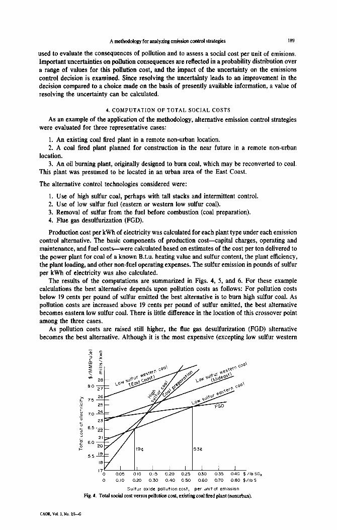
The results of the computations are summarized in Figs. 4, 5, and 6. For these example calculations the best alternative depends upon pollution costs as follows: For pollution costs below 19 cents per pound of sulfur emitted the best alternative is to bum high sulfur coal. As pollution costs are increased above 19 cents per pound of sulfur emitted, the best alternative becomes eastern low sulfur coal. There is little difference in the location of this crossover point among the three cases.

As pollution costs are raised still higher, the flue gas desulfurization (FGD) alternative becomes the best alternative. Although it is the most expensive (excepting low sulfur western

:;: 0 0.05 010 0.15 0.20 0.25 0.30 0.35 0.40 $ /I b SO,

0 0.10 0.20 0.30 0.40 0.50 0.60 0.70 0.60 $/lb S

Sulfur oxide pollution cost, per unitof emission

Fig. 4. Total social cost versus pollution cost, existing coal tired plant (nonurban).

CAOR, Vol. 3, No. 2/3-G


0 0.05 0. I 0 0.15 0.20 0.25 0.30 035 CI40 $/lb SO,

0 0.10 0.20 0.30 0.40 0.50 0.60 0.70 0.60 $/lb S

Sulfur oxide pollution cost, per umtof emission

Fig. 5. Total social cost versus pollution cost, new coal fired plant (nonurban).

_ % f s 6.5

6.0

17 I I I I I

0 0.05 0.10 0.15 0.20 0.25 C I I I I I I? 10 0.35 0.40 0.45 0.50 $/lb SOx

0 0.10 020 030 0.40 0.50 0.60 070 000 0.90 1.00 $/lbS


Fig. 6. Total social cost versus pollution cost, old coal fired plant reconverted to coal (urban)

coal) the FGD alternative permits overall emissions reductions approaching 90%, whereas low sulfur eastern coal gives only a 70% reduction. The added cost for the additional sulfur removal may be substantial, so that the cross-over points where FGD drops below low sulfur eastern coal are high: 53 cents per pound of sulfur for the retrofit non-urban plant (Fig. 4), 37 cents for the new non-urban plant (Fig. 5), and 59 cents for the retrofit urban plant (Fig. 6).

5. ESTIMATION OF POLLUTION COSTS

Application of the methodology has converted the decision of which sulfur control alternative to use to a judgment of the societal costs of sulfur emissions. The usefulness of our decision model therefore depends on our ability to convert accurately a given level of sulfur oxide emissions to a pollution cost in dollars. The framework for this conversion is illustrated in Fig. 2 by those components of the diagram to the right of the block marked “Containment of Emissions”.

6. DISPERSION MODEL

In the absence of quantitative relationships between sulfur oxide emissions and ambient sulfate levels available for the National Academy study, a simple model for atmospheric


transport and conversion was developed. The model was based on the following assumptions:

I. In a period shortly following the emission, the sulfur oxides become uniformly distributed from the ground to a mixing layer height. The height of the plume then remains constant.

2. The emissions are uniformly distributed over an arc of constant size, so that the width of the plume expands in direct proportion to the time since emission, or (with constant wind velocity) in direct proportion to the distance downwind travelled by the plume.

3. The emissions travel down the plume un~ormly distributed in a “box” whose length is the distance travelled by the wind per unit time, whose height is the height of the mixing layer, and whose width is the distance perpendicular to the wind direction subtended by an angle of constant size. Thus, the width of the box grows in direct proportion to time, and the concentration of pollutants decreases inversely with time.

The following assumptions were made about the chemical reactions of the sulfur oxides.

1. Sulfur dioxide to sulfate oxidation takes place according to a first order rate reaction. The rate may change considerably between comparatively clean rural air and pollutant-laden urban air.

3. Sulfur dioxide is removed to the ground at a constant deposition velocity, ~ginning at the time of emission. (This assumption will overestimate the amount of sulfur dioxide removal to ground for a plume from a tall stack that travels many miles before touching ground, and it will underestimate the sulfur dioxide removal from a shorter stack where the plume is in contact with the ground for substantial time before the plume is dispersed uniformly up to the inversion or mixing layer height).

3. Suspended sulfate is removed to the ground at a constant deposition velocity, beginning with the time of emission.

The model was used to examine two representative situations:

1, A plant in a remote rural location, approximately 500 km upwind of a major metropolitan area,

2. A plant located in a metropolitan area, with urban settlement extending 40-80 km downwind from the plant.

The first was used to examine both an existing coal fired plant and a new coal fired plant in a remote location, and the second to examine an existing plant in an urban location that could be reconverted from oil to coal.

The following values were used as inputs to the calculation:

1. The wind is a constant 20 km/h. 2. The angle subtended by the plume is IS”. 3. The height of the mixing layer above ground is 1000 m. 4. The deposition velocity of sulfur dioxide to the ground is 0.8 cm/s, giving a removal rate of

2.88% per h with a mixing layer height of 1000 m above ground. 5. The deposition velocity of SO, to the ground is 0.4 cm/s, giving a removal rate of 144% per

h with a mixing layer height of 1000 m. 6. The oxidation rate of sulfur dioxide to form sulfates is 0.5% per h in rural air outside of a

metropolitan area, and 5.0% when the air has passed over a metropolitan area and contains particulates, oxidants, and hy~oc~~ns from urban emission sources.

7. All sulfur oxides emitted from the power plant are emitted as sulfur dioxide rather than as sulfates. Assuming 1 to 2% of SO, is emitted as sulfate, the error introduced by this approximation is negligible.

We shall su~~ize the results for the case of a remotely located power plant of about 600 MW, burning 3% sulfur coal. Its average emission level (including the effect of plant loading) was computed to be lo4 kg of sulfur dioxide per h. Plant emissions were assumed to encounter polluted urban air in a metropolitan area480 km (300 miles) downwind after 24 h. At this time it was assumed that the oxidation rate changed from 0.5 to 5% per h.

The results of the calculations are shown in Fig. 7. Notice that the change in sulfur dioxide oxidation rate for urban air causes a sharp rise in the incremental contribution to sulfate levels within the urban area.

192 D. WARNER NORTH and hf. W. MERKHOFER

s 25 -

t- z

SO, contribution

Time In hr since emission

Fig.7. Incremental contributions to ambient levels of SO, and sulfate from the emissions of a single power plant, representative calculation for 600 MW plant 300 miles upwind of urban area.

A detailed assessment of health, materials, damage, and other consequences would include the spatial variation in the ambient levels of sulfur dioxide and sulfate. We have avoided this level of detail and used representative single values for the incremental contribution to ambient sulfur dioxide and sulfate levels resulting from the emissions of the power plant. For the remotely located plant, we have taken as representative for computing pollution consequences the values after two hours of oxidation in urban air (following 24 h in rural air to give a total of 26 h since emission from the power plant). For the urban plant, we have taken as representative the values three hours after emission, assuming oxidation in urban air during this time. The values resulting from the calculation are given in Table 1.

A sensitivity analysis, Table 2, shows the effects of changes in inputs to the model. The sensitivity values have been chosen rather subjectively by the authors as representing a set of reasonable extreme values. The dominant effect of the oxidation rates in determining the ambient sulfate concentration shows up strongly in the table. Depending on whether we use high or low values, we get about an eightfold change in the contribution to ambient sulfate levels from the power plant.

As a rough approximation for assessing the uncertainties involved, we have assumed that the extreme values represent approximately the 5% and 95% points on a cumulative probability distribution assigned to the quantity (i.e., the probability is judged to be 90% that the uncertain quantity would lie in the interval between the low and high values used in the sensitivity analysis, rather than outside the interval). In addition, uncertainties are assumed independent, except for the rural and urban oxidation rates which are assumed totally dependent (e.g., if one is high then the other will be high also, and vice versa). A sketch of the resulting probability distribution on ambient sulfate levels is given in Figs 8 and 9. These curves are meant to illustrate the great uncertainty on the incremental change in ambient sulfate levels resulting from the

Table 1. Emissions to ambient calculation for representative power plants (emissions rate assumed is 1O’kg of sulfur dioxide per h)

Case

Increase in ambient concentration, &m3 SO, Sulfate

Location of measurement

Oxidation rate

assumption

Remotely located plant (existing or new plant)

Urban plant (existing plant)

1.39 0.58

25.0 6.2

Urban area 26 h (520 km) downwind

Urban area 3 h (60 km) downwind

24 h at 0.5% then 2 h at 5%/h

3 h at 5%/h

A methodology for analyzing emission cet&ol strategies

Table 2. Sensitivity analysis, emissions to ambient relationship

Remote plant, after 26 h Urban plant, after 3 h

SO, cone, SO, cone, SO2 cone, SO. cone, pg/m’ w/m’ M/m’ &m3

Nominal values 1.39 0.58 25.0 6.20 low oxidation rate

0.1% h in rural per air 1.6 0.13 28.2 1.32 1.0% per h in urban air

High oxidation rate 1.0% h in rural per air 1.1 1.06 21.5 11.6 10.0% per h in urban air

With constant 2% 1.03 1.30 21.3 2.59 oxidation rate SO, deposition rate

Low: 0.4 cm/s 2.0 0.74 26.1 6.33 High; 1.6 cm/s 0.7 0.38 22.9 5.95

SO. deposition rate Low: 0.03 cm/s 1.4 0.67 25.0 6.32 High: 0.8 cm/s 1.4 0.51 25.0 6.07

Height of mixing layer Low: 5OOm 1.3 0.64 45.8 11.6 High: 15OOm 1.2 0.48 17.2 4.27

Angle subtended by plume Low: lo” 2.1 0.88 37.6 9.33 High: 22.5” 0.9 0.39 16.5 4.10

193

IO-

06-

Meanx0.58pg/m3

Standard deviation

I I I I I I I I 0 0.2 0.4 06 0.8 1.0 1.2 1.4 1.6 I.6

Ambient sulfate concentration increment, pg/m3

Fig. 8. Sketch of probability distribution illustrative of present uncertainty on increment of ambient sulfate concentration in urban area approximately 300 miles (500 km) downwind of rural power plant emitting 10’ kg

of sulfur oxides per h.

emissions from a power plant located upwind from an urban area in which there are substantial health and material property values at risk. More refined models, formal probability assessment procedures, and formal probability processing could be used to improve the degree to which these curves summarize present knowledge on the emissions-to-ambient relationship for sulfates. The curves shown may be taken as rough summaries of the present state of knowledge, and they are subject to revision as further information is obtained.

7. EXPOSURE MODEL

In determining the population at risk, two additional factors must be incorporated into the dispersion model: (1) variations in wind direction, and (2) loss due to wet deposition of sulfur dioxide and sulfate.

Whereas 15” may be an appropriate value for the angle subtended by the plume on a particular

D. WARNER NORTH and M. W. MERKHOFER

Amblent sulfate concentration increment, pg/m3

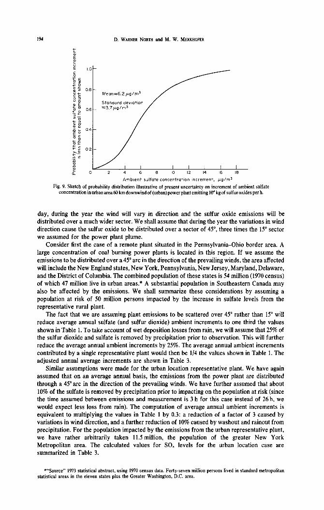
Fig. 9. Sketch of probability distribution illustrative of present uncertainty on increment of ambient sulfate concentration in urban area 60 km downwind of (urban) power plant emitting 10’ kg of sulfur oxides per h.

day, during the year the wind will vary in direction and the sulfur oxide emissions will be distributed over a much wider sector. We shall assume that during the year the variations in wind direction cause the sulfur oxide to be distributed over a sector of 45”, three times the 15” sector we assumed for the power plant plume.

Consider first the case of a remote plant situated in the Pennsylvania-Ohio border area. A large concentration of coal burning power plants is located in this region. If we assume the emissions to be distributed over a 45” arc in the direction of the prevailing winds, the area affected will include the New England states, New York, Pennsylvania, New Jersey, Maryland, Delaware, and the District of Columbia. The combined population of these states is 54 million (1970 census) of which 47 million live in urban areas.* A substantial population in Southeastern Canada may also be affected by the emissions. We shall summarize these considerations by assuming a population at risk of 50 million persons impacted by the increase in sulfate levels from the representative rural plant.

The fact that we are assuming plant emissions to be scattered over 45” rather than 15” will reduce average annual sulfate (and sulfur dioxide) ambient increments to one third the values shown in Table 1. To take account of wet deposition losses from rain, we will assume that 25% of the sulfur dioxide and sulfate is removed by precipitation prior to observation. This will further reduce the average annual ambient increments by 25%. The average annual ambient increments contributed by a single representative plant would then be l/4 the values shown in Table 1. The adjusted annual average increments are shown in Table 3.

Similar assumptions were made for the urban location representative plant. We have again assumed that on an average annual basis, the emissions from the power plant are distributed through a 45” arc in the direction of the prevailing winds. We have further assumed that about 10% of the sulfate is removed by precipitation prior to impacting on the population at risk (since the time assumed between emissions and measurement is 3 h for this case instead of 26 h, we would expect less loss from rain). The computation of average annual ambient increments is equivalent to multiplying the values in Table 1 by 0.3: a reduction of a factor of 3 caused by variations in wind direction, and a further reduction of 10% caused by washout and rainout from precipitation. For the population impacted by the emissions from the urban representative plant, we have rather arbitrarily taken 11.5 million, the population of the greater New York Metropolitan area. The calculated values for SO, levels for the urban location case are summarized in Table 3.

*“Source” 1973 statistical abstract, using 1970 census data. Forty-seven million persons lived in standard metropolitan statistical areas in the eleven states plus the Greater Washington, DC. area.


Table 3. Summary of judgment for average amtual ambient increases of sulfur oxide and population at risk assumptions for representative power plant case analyses

Representative Average annual power plant with Ambient increase from ambient increases Population at risk

emissions of lo’ kg of plant emissions for a Average loss from from plant emissions assumed with 45” SOJh or %,XKl tons 15” angle plume, from wet deposition of assuming distribution sector for

of SO, per year Table 1 sulfur oxides over a 45” sector representative case

Remote location (+$

Sulfate W5;7

(Ambient increase ’ ’ measured 26 h or 52Okm downwind)

Urban location 25.0 6.2 (Ambient increase measured 3 h downwind)

25%

10%

Sulfate

(zz)

1.86

50 million

11.5 million

8. HEALTH EFFECTS MODEL

A number of epidemiological studies suggest that short-term exposures to elevated levels of sulfur oxides

1. aggravate pre-existing heart and lung disorders in elderly patients, 2. aggravate asthma, and 3. perceptibly increase daily mortality.

Repeated short-term exposures or elevations of annual average exposures seem to 4. increase the incidence of lower respiratory disease in children, 5. increase the risk for chronic respiratory disease in adults.*

Considerably more research is required before any definite quantitative relationship may be established. However, progress is being made in this area, and it is useful to demonstrate the manner in which dose-response curves should be utilized in the context of the sulfur oxide pollution control decision problem.

As a crude approximation we have assumed that each of the above health effects is characterized by a linear threshold relationship. The approximation is that no adverse health effect results below some threshold level of suspended sulfate concentration. Above this level, the percent of cases of the adverse health effect which may be attributed to the sulfate (the “percent excess”) is assumed to increase linearly with concentration. By plotting the results of various epidemiological studies on a graph relating the percent excess of health effects to levels of suspended sulfates, the “best fit” for such a linear-threshold relationship may be obtained. The results of such a curve fitting exercise and the studies upon which they were based are summarized in Table 4.

Once dose-response curves have been agreed upon, they may be combined with expected frequency distributions of suspended sulfate concentrations to obtain an estimation of the health effects expected from an increase in the current ambient levels of suspended sulfates.

Using this method, an estimate was made of the health effects of a 1 pglm’ increase in the annual average level of suspended sulfate concentration in the New York Metropolitan area. Daily concentrations of ambient suspended sulfate concentrations were assumed to follow a lognormal frequency distribution with an annual average of 16 H/m” and a standard deviation of 5.6 pg/m3. This assumption is consistent with the New York studies of the CHESS [3] report. The results are summarized in Table 5. Since annual average concentrations may differ from 16 M/m’, depending upon exact location, the calculations were also performed assuming annual average concentrations of 12.5 and 20 w/m’. The last column of Table 5 gives the expected number of additional cases resulting from a 1 fig/m’ annual average sulfate concentration increase. There are, of course, considerable uncertainties in these estimates. The uncertainty in health effects will be addressed below.

*For a thorough discussion see part one: health and ecological effects of sulfur dioxide and sulfates, in Ref. [l].

196 D. WARNER NORTH and hi. W. MERKHOFER

Table 4. “Best judgment” dose-response functions*

Adverse health effect

Best judgment threshold function Exposure Threshold duration &g/m’) Slopet

Increased daily mortality Aggravation of heart

and lung disease Aggravation of asthma Excess lower

respiratory disease in children

Excess risk for chronic resp. disease in adults+

24 h or longer 25 0.252

24 h or longer 9 1.41 24 h or longer 6 3.35

Up to 10 years 13 7.69

Up to 10 years 12 11.1

*These dose response relationships were developed in an unpublished study for the U.S. Environmental Protection Agency. The “best judgment threshold functions” represent subjective approximations to data, not precise mathematical fits. The studies upon which the estimates were based are as follows: Mortality; Refs. [4-IO]. Aggraoation of heart and lung disease; Refs. [li, 121. Aggravation of asthma; Refs. [13-151. Excess lower respiratory disease in children; Refs. [16-221. Excess chronic respiratory disease; Refs. [23-301.

tChange in percent excess over base rate for population, per pdrn’ change in suspended sulfate level.

SFor chronic respiratory disease, difficulties with available data necessitated the unit of measurement*to be excess risk rather than direct incidence of illness. Actually, in its originally calculated form, separate dose response functions were assessed for cigarette smokers and non-smokers. The function described in the table is a weighted linear average based upon the average prevalence of cigarette smoking in the adult population at risk.

Table 5. Estimates of adverse health effects attributable to a 1 &m’ increase of average suspended sulfates in the New York Metropolitan area

Health effect

Average number

of cases* (million)

Cases attributable to suspended SO, concentration

at average con;;;;;on at average concentration + 1 pg/m’ percent percent number additional

cLslm’ of cases of cases of cases of cases expected cases

Increased daily 0.118 million 12.5 0.0418 49.4 0.0512 60.5 11.1 mortality Deaths/year 16.0 0.0839 99.2 0.1031 121.9 22.7 (premature deaths per yr.) 20.0 0.1919 226.9 0.2350 277.9 51.0

Aggravation of 12.5 5.829 1.422 6.902 1.684 0.262 heart and lung disease 24.4 16.0 9.907 2.417 11.569 2.823 0.406 (million person-days per yr.) 20.0 15.137 3.693 16.903 4.124 0.431

Asthmatic attacks 12.5 22.29 0.5595 25.50 0.6401 0.0806 (millions per year) 2.51 16.0 33.48 0.8404 36.83 0.9245 0.0841

Lower respiratory 20.0 46.88 1.1768 50.23 1.2609 0.0841 disease in children 12.5 0 0 3.815 4.85 4.85 (thousands of cases per year) 127 16.0 23.04 29.2 30.73 39.10 9.90

Chronic respiratory 20.0 53.80 68.5 61.49 78.20 9.90 disease symptoms 12.5 7.75 0.0284 18.85 0.0690 0.0406 (millions of cases, 0.366 16.0 46.60 0.1707 57.70 0.2113 0.0406 point prevalence) 20.0 91.00 0.3333 102.10 0.3739 0.0406

*The figures cited under “average number of cases” are estimates based upon data from the Statistical Abstract of the U.S., 1970, and information on health effect prevalence rates. The prevalence rates used are as follows: (1) annual death rate (per 1OOO); 10.2, (2) prevalence of heart and lung disease in elderly persons; 0.27, average number of aggravated days per day person; 0.20, (3) asthma prevalence rate; 0.03 (Prevalence of selected chronic respiratory conditions U.S.-1970), attacks per day per asthmatic; 0.02, (4) annual incidence rate for lower respiratory disease in children; 0.06 (Acute conditions-incidence and associated disability U.S. 1971-72), (5) chronic respiratory disease prevalence rate; 0.02 for non-smokers (62%) and 0.10 for smokers (38%) (Prevalence of selected chronic respiratory conditions-1970, Archives of Environmental Health, Vol. 27, Sept. 1973).

Health cost model The nominal values chosen in the analysis to represent the costs to society of each incidence

of an adverse health effect are summarized below.

Estimation of per case health costs One premature death = $3O,ooo


One day aggravation of heart and lung disease symptoms One asthma attack One case child’s lower respiratory disease One case chronic respiratory disease

= $20 = $10

= $75

= $250

Ideally, these values should be assigned so as to reflect what society would (or should) just be willing to pay in dollars to prevent the losses sustained when a typical individual suffers one of the possible health effects. The authors believe that medical cost and lost productivity should not be the only basis for assessing these values. Since there may be considerable disagreement on what the dollar assignments should be, the sensitivity of results to these values must be carefully checked.

Although expressing health losses in terms of the dollar is convenient for our purposes, other common units of measurement are possible. One other popular numeraire of estimating health damages is the “equivalent day of restricted activity (EDRA)” (Jacoby et af.[31]). The Public Health Service[32] defines a day of restricted activity as one on which a person substantially reduces the amount of activity normal for that day because of specific illness or injury. If we assume a person-day of restricted activity to imply health costs of between $1 and $10, our nominal health costs compare well with the estimations of Jacoby et a1.,[31, Table 8-41.

For premature death we have used a value of $30,000. Most of the deaths occur among chronically ill elderly people, and the amount by which their lives are reduced may be only a matter of days or weeks. It is not known whether sulfate levels have any correlation with the general reduction in life expectancy for persons of average age and health. Rather, the effect observed is a statistical increase in number of deaths recorded on days of high pollution levels vs days of low pollution levels. For this reason we have used a value of $30,000 per life rather than the value of the order of $200,000 used in highway safety and other applications for the value of life for a representative individual in the population[33]. Sensitivity analysis indicates that results are not dependent on the value assigned to premature death.

Multiplication of per-case health costs times the number of cases given in Table 5 yields the total yearly health costs resulting from a 1 pg/m’ increase in suspended sulfate concentration in the New York Metropolitan area. A sensitivity analysis was conducted to determine the sensitivity of this value to the various assumptions of the health model. The results are shown in Table 6.

The sensitivity values shown in Table 6 have been chosen somewhat arbitrarily as representing a set of reasonable extreme values. The low and high values for the change in incidence of each health effect, per unit change of ambient sulfate, were taken to be 10 and 200% of the nominal values respectively.

The indication from the sensitivity analysis is that the most critical quantities in the assessment of the total health cost of a 1 pg/m3 increase in suspended sulfate concentration are the number of additional cases of chronic respiratory disease and the number of additional person-days of aggravated heart-lung disease symptoms. As a rough approximation for assessing the uncertainty in health costs we neglected all uncertainties but those arising from these two most critical variables.

The uncertainties in the number of additional cases of chronic respiratory disease and the number of additional days of aggravation from heart and lung disease symptoms were judged to be such that there is only one chance in ten that each of these quantities lies outside the interval defined by the low and high values used in the sensitivity analysis. Specifically, we assumed that there is only a 5% chance that the additional number of cases of chronic respiratory disease from a 1 pg/m’ increase in SO, is less than 4050, and a 5% chance that this number is greater than 81,200. Further, these uncertainties were assumed to be totally dependent (i.e. if the additional number of cases of chronic respiratory disease is high, then the number of additional days aggravation from heart and lung disease will also be high, and vice versa). Similarly, we assumed that there is a 5% chance that the number of additional days of aggravation from heart and lung disease is less than 41,000 and a 5% chance that this number exceeds 820,000. Finally, in order to facilitate the calculations, we assumed that the probability distribution characterizing the resulting uncertainty


Table 6. Sensitivity analysis: total health cost of a 1 pg/m’ increase in average suspended sulfate concentration in the New York Metropolitan area

Total health cost per pglm” SO,

(million $)

Nominal values Additional premature deaths low: 2.3 high: 46 Additional days of aggravated heart and lung disease low: 0.041 miIhon/yr. high: 0.82 million/yr. Additional asthmatic attacks low: 8.4 thousand/yr. high: 168 thousand/yr. Additional cases lower respiratory disease in children low: 0.99 thousand/yr. high: 19.8 thousand/yr. Additional cases chronic respiratory disease low: 4.06 thousand/yr. high: 81.2 thousand/yr. Cost per premature death low: $3000 high: $120,000

20.5

19.9 21.2

13.2 28.6

19.7 21.3

19.8 21.2

11.3 30.7

19.9 22.5

Cost per day of aggravation of heart and lung disease symptoms low: $2 high: $80 Cost per asthma attack low: $1 high: $40 Cost per case child’s lower respiratory disease low: $7.50 high: $300 Cost per case chronic respiratory disease low: $25 high: $1000

13.2 44.8

19.7 23.0

19.8 22.7

11.3 51.1

in health’ cost is a lognormal distribution. The shape of this distribution makes it a good approximation; however, greater accuracy could be obtained by formally assessing the subjective distributions of experts in the area of health effects. Procedures for such probability assessments exist (cf. Spetzler and Stail von Holstein[34]).

The resulting probability distribution characterizing the uncertainty of the total health costs of a 1 fig/m’ increase in average annual ambient sulfate concentration in the New York Metropoli- tan area is illustrated in Fig. 10.

IO- Mean= $16m1Ilion

06-

0 IO 20 30 40 50

Total health cost per &g/m3 increase I” sulfate concentration, ml/lion $

Fig. 10. Probability distribution illustrative of present uncertainty on total health cost due to a 1 w/m’increase (from an ambient level of 16 clp/m’) in annual average suspended sulfate concentration for the New York

Metropolitan area. Population at risk: 11.5 million.

A methodology for analyxing emission control strategies

9. ECOLOGICAL DAMAGE AND COST MODEL

199

Acid rain resulting from sulfur oxide and nitrogen oxide emissions is now widespread over Northern Europe and the Northeastern United States. (Ch. 7 of Ref. [l]). The consequences may include acidification of soils, loss of growth in forests, death of fish from low pH in lakes and streams, and damage to outdoor statues and building facades. These effects are ditbcult to assess in economic terms, but they do not seem significant compared to the potential health effects discussed above.

We have therefore chosen arbitrarily a value for the overall costs associated with acid rain of $500 million annually, which is equivalent to about 1.5 cents per pound of sulfur emitted (with 1970 emission levels). As shown below, sensitivity analysis indicates that the costs ascribed to aesthetics and acid rain have little effect on the overall result for the total pollution cost per pound of sulfur emitted.

10. MATERIAL DAMAGE AND COST MODEL

Waddell[35] has assessed the national SO,-related material damage costs in 1970 to lie between $0.4 billion and $0.8 billion. Although the total national sulfur oxide pollution damage is a useful number, it does not help us much if we are trying to judge between various pollution reduction strategies. What we really need to know is the sensitivity of pollution damage to pollution levels.

Unfortunately, as is the case with health effects, little is known about pollution versus material damage dose-response relationships. Degradation of concrete and metal building materials, paints, and fibers, account for most of the estimated damage. The mechanism by which pollution contributes to this damage is not entirely clear. Rates of deterioration appear to be functions of sulfate accumulation, implying that there is no ambient sulfate level below which no effect will occur.* The relative significance for damage of the various atmospheric sulfur compounds are not known.

We have summarized our available information into a crude dose-response model. Assume that most material damage occurs in Northeastern urban areas and let us take as the average Northeastern urban concentrations 60 &m3 sulfur dioxide and 16 pg/m’ suspended sulfate. The model consists of a linear approximation to material costs about these concentrations. Let f be the fraction of the estimated sulfur oxide materials damage cost which is due to exposure to sulfur dioxide and let the remaining fraction, l-f, be the result of exposure to suspended sulfates. The net change in urban material damage costs, denoted MD, for a given change k, in average sulfur dioxide concentration and a given change kz in average sulfate concentration, is then assumed to be given by

tMD = fi pg/m” + (1 - f) 2 w/m31 x Total SO, material cost for the area.

Following the method of analysis in the previous section on health costs, we wish to estimate the effect that a 1 cLglrn3 increase in ambient sulfate concentration will have on material damage costs. In the absence of more detailed information we shall proceed as follows: We begin with Waddell’s[35] estimate of $600 million for annual materials damage caused by sulfur oxides to material property, which applies to the nation as a whole. We have assumed that 90% of this damage occurs in the Northeastern United States: 60% in the New England States-New York, Pennsylvania, Maryland, New Jersey, Delaware, and Greater Washington, D.C.-and 30% elsewhere east of the Mississippi River. In the above mentioned states we have assumed that the materials damage from sulfur oxides for an area is proportional to its population; most of the sulfur oxide damage to materials such as paints and metals will occur primarily in urban areas. We have assumed, as earlier, that the population at risk for the remotely located plant (assumed

*However, as Giiette[36] points out, while physical deterioration of materials may occur at relatively low pollution levels, for the effects to be economically important (1) the normal service life of the material must be reduced, (2) the frequency of maintenance tasks must be increased, or (3) the quality of the services rendered by the product must be diminished. For this reason, while a threshold may not exist for physical damage, economic loss from physical damage may exhibit such a threshold. Our analysis ignores this effect, possibly causing us to underestimate marginal material damage costs. More accurate dose-response information ought to be applied in the analysis as it becomes available.


in the Pennsylvania/Ohio border-West Virginia area) is 50 million, and that total sulfur oxide materials damage in the area affected by this plant (the states mentioned above) is 60% of $600 million, or $360 million per year. For the urban representative plant, the population at risk was assumed to be 11.5 million, so the total sulfur oxide materials damage was estimated as (1 l.S/SO) x 60% x 600 = $83 million per year.

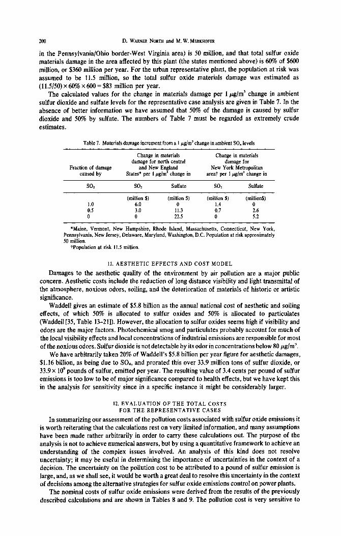
The calculated values for the change in materials damage per 1 pg/m’ change in ambient sulfur dioxide and sulfate levels for the representative case analysis are given in Table 7. In the absence of better information we have assumed that 50% of the damage is caused by sulfur dioxide and 50% by sulfate. The numbers of Table 7 must be regarded as extremely crude estimates.

Table 7. Materials damage increment from a 1 pg/m’ change in ambient SO, levels

Fraction of damage caused by

SO,

Change in materials Change in materials damage for north central damage for

and New England New York Metropolitan States* per 1 H/m’ change in areat per 1 N/m’ change in

SO* Sulfate SO* Sulfate

(million $) (million $) (million $) (millionS) 1.0 6.0 0 1.4 0 0.5 3.0 11.3 0.7 2.6 0 0 22.5 0 5.2

*Maine, Vermont, New Hampshire, Rhode Island, Massachusetts, Connecticut, New York, Pennsylvania, New Jersey, Delaware, Maryland, Washington, D.C. Population at risk approximately 50 million.

tPopulation at risk 11.5 million.

11. AESTHETIC EFFECTS AND COST MODEL

Damages to the aesthetic quality of the environment by air pollution are a major public concern. Aesthetic costs include the reduction of long distance visibility and light transmittal of the atmosphere, noxious odors, soiling, and the deterioration of materials of historic or artistic significance.

Waddell gives an estimate of $5.8 billion as the annual national cost of aesthetic and soiling effects, of which 50% is allocated to sulfur oxides and 50% is allocated to particulates (Waddell [35, Table 13-211). However, the allocation to sulfur oxides seems high if visibility and odors are the major factors. Photochemical smog and particulates probably account for much of the local visibility effects and local concentrations of industrial emissions are responsible for most of the noxious odors. Sulfur dioxide is not detectable by its odor in concentrations below 80 pg/m’.

We have arbitrarily taken 20% of Waddell’s $5.8 billion per year figure for aesthetic damages, $1.16 billion, as being due to SO,, and prorated this over 33.9 million tons of sulfur dioxide, or 33.9 x lo’ pounds of sulfur, emitted per year. The resulting value of 3.4 cents per pound of sulfur emissions is too low to be of major significance compared to health effects, but we have kept this in the analysis for sensitivity since in a specific instance it might be considerably larger.

12. EVALUATION OF THE TOTAL COSTS FORTHEREPRESENTATIVECASES

In summarizing our assessment of the pollution costs associated with sulfur oxide emissions it is worth reiterating that the calculations rest on very limited information, and many assumptions have been made rather arbitrarily in order to carry these calculations out. The purpose of the analysis is not to achieve numerical answers, but by using a quantitative framework to achieve an understanding of the complex issues involved. An analysis of this kind does not resolve uncertainty; it may be useful in determining the importance of uncertainties in the context of a decision. The uncertainty on the pollution cost to be attributed to a pound of sulfur emission is large, and, as we shall see, it would be worth a great deal to resolve this uncertainty in the context of decisions among the alternative strategies for sulfur oxide emissions control on power plants.

The nominal costs of sulfur oxide emissions were derived from the results of the previously described calculations and are shown in Tables 8 and 9. The pollution cost is very sensitive to


Table 8. Cost of sulfur oxide emissions: representative calculation for remote plant emitting 10,000 kg of SO, per h (%.5 x l(P pounds of sulfur per year)

Costs computed based on 0.145 pg/m’ ambient increase in sulfate and 0.35 M/m’ ambient increase in sulfur dioxide in metropolitan areas with a population of 50 million

Health effects (computed at ambient level of 16 M/m’) 25,600 cases of chronic respiratory

disease x $250 per case 256,000 person-days of aggravated heart-lung

disease symptoms x $20 53,ooO asthma attacks x $10 each 6200 cases of children’s respiratory

disease x $75 14 premature deaths x $30,000

Total health costs

$6.4 million

5.1 0.5

0.5 0.4

- 12.9

Materials damage $11.3 million per drn” of SO, X 0.145 1.6 $3.0 million per w/m’ of SO, X 0.35 1.1

Aesthetics ($0.034 x %.5 x 10” Ibs) 3.3 Acid rain ($0.015 x %.5 x lo” Ibs) 1.4

Total emissions costs $20.3 million Emissions cost per pound of sulfur 216

Table 9. Cost of sulfur oxide emissions: representative calculation for urban plant emitting 10,000 kg of SO, per h (%.5 x 106pounds of sulfur per year)

Costs computed based on 1.86 M/m’ increase in sulfate and 7.5 drn’ increase in sulfur dioxide concentrations in metropolitan areas with population of 11.5 million.

Health effects from increase: (computed at ambient level of 16 &m3) 75,500 cases of chronic respiratory disease

x $250 per case $18.9 million 755,000 person days of aggravated heart-lung

disease symptom x $20 per day 15.1 156,000 asthma attacks at $10 each 1.6 18,400 cases of children’s lower 1.4

respiratory disease at $75 1.3

Total health costs $38.3 million

Materials damage 2.6 million per pg/rn3 of SO, x 1.86 4.8 0.7 million per &ml of SO, x 7.5 5.3

Aesthetics ($0.034 x %.5 x lo” Ibs) 3.3 Acid rain etc. ($0.015 x %.5 x lo” Ibs) 1.4

Total emissions costs $53.1 million Emissions costs per pound of sulfur 556

many of the input values assumed for the analysis. A list of selected sensitivity calculation results is given in Table 10; appropriate ranges for these calculations were estimated from information available to the National Academy study team [ 11.

The dominant terms contributing to the uncertainty in pollution costs are the uncertainty on the ambient increase in urban sulfate resulting from the emissions of a single power plant (Figs. 8 and 9) and the health effects of a given ambient sulfate increase on incidence of chronic respiratory disease and aggravation of heart-lung disease symptoms (Fig. 10). Therefore, the probability distribution on the product provides a first cut assessment of the overall uncertainty on pollution cost. In this way, the probability distributions on urban sulfate levels and the effects of a 1 pg/m3 increase in urban sulfate concentrations were used to compute overall probability distributions on pollution cost per pound of sulfur emitted.

The Figs. 11, 12, and 13 are copies of Figs. 4, 5, and 6 showing the total social cost per kWh for the representative plant as a function of the cost per pound of sulfur emitted. We show the

Nominal value

0.5%/h-r& air 5.0%/h-urban air

3530 per million population

$250

$20

$75

$10

$30,000 *

202 D. WARNER NORTH and M. W. MERKHOPER

Table 10. Selected sensitivity analysis

Factor

Oxidation rate of so* to so,

Oxidation rate constant at 2%

Increase in incidence of chronic respiratory disease, per ambient increase of lpg/m’ of SO,

Increase in incidence of all health effects, per ambient increase of 1 cLp/m’ of SO,

Value assigned to case of chronic respiratory disease

Value assigned to day of aggravated heart-lung disease symptoms

Value assigned to case of child’s lower respiratory disease

Value assigned to asthma attack

Value assigned to premature death

All health values

Sensitivity range

O.l-1.0% l.O-10.0%

IO-200% of nominal

lo-200% of nominal

$lOO-$1000

$lO-$80

$25-$225

U-$50

$lO,OoO-$200,000 lo-400%

of nominal

Range in pollution

cost (e/lb S) remote plant urban plant

9.5-33 21-93

39 30

15-28 31-15

9-34 19-95

17-41 43-114

18-37 47-102

21-22 54-58

21-23 54-62

21-24 54-62 9-61 19-174

> 25- : .u ; : u g ‘, 8

2 Probability

t” density function

19q for pollution cost (Rural case)

53$

A- l 1 I I I

0 0.10 0,20 0.30 0.40 0.50 0.60 0.70 0.80 $ /IbS


Fig. 11. Total social cost versus pollution cost, existing coal fired plant (nonurban), showing probability distribution on pollution cost per pound of sulfur.

probability distribution on pollution cost plotted as a probability density function. The height of the curve is the likelihood of various values of the pollution cost. The area under the curve between any two values for the pollution cost corresponds to the probability that the pollution cost would lie in that interval, were the uncertainty to be resolved.


J.G 0 z 194 37c

t

s 21 - Probability density function

;5 6.0 -- z 20 -

for pollution cost

5.5 19 -

--

18 -

-I- I- I I I

0 0.05 0.10 0.15 0.20 0.25 0.30 0.35 0.40 $ /I b SO,

0 0.10 020 0.30 0.40 0.50 0.60 0.70 0.80 $/lbS


Fig. 12. Total social cost versus pollution cost, new coal fired plant (non-urban), showing probability distribution on pollution cost per pound of sulfur.

0 0.10 0.20 0.30 0.40 0.50 0.60 0.70 0.80 0.90 100 $/lbS


Fig. 13. Total social cost versus pollution cost, old coal fired plant reconverted to coal (urban), showing probability distribution on pollution cost per pound of sulfur.

13. THE VALUE OF RESOLVING UNCERTAINTY

The decisions on control strategy depend on the adequacy of the information available at the time the decision must be made. There is great value to improving our information about certain aspects of sulfur oxide pollution. The value of resolving uncertainty derives from the idea that better information might show, for example, that pollution costs are lower than was estimated, and costly abatement methods are not warranted. With some probability, then, their extra cost might be saved. In particular, a better understanding of the health effects of sulfates and of the chemistry of the conversion of sulfur dioxide to atmospheric sulfates could have a significant effect on future decisions on control of sulfur oxides.

An important consequence of the decision analysis formulation of this problem is that it allows us to determine the value of resolving uncertainty. The value of resolving uncertainty is the difference between the value of the decision situation where information will be made

204 D. W~~~ NORTH and M. W. MERKHOFER

available to resolve the uncertainty before the decision is made, and the value of the decision situation where the decision must be made in the face of uncertainty. (The concept of the value of information is a basic and rather subtle idea in modern decision theory, See, for example, Howard[37], North[38], Raiffa,[391, Tribus[40] for a detailed explanation of the concept and the computation).

Table 11 summarizes the computed values of eliminating unce~ainty on the emissions-to- ambient relationship and on the health consequences of sulfate. The computations were performed both with and without the assumption that low sulfur eastern coal is an available alternative.

There are at least the equivalent of about one hundred of our representative rural plants (~,~MW) burning approximately 3% sulfur coal in the Northeastern region of the United States[41]. In addition there are about 40,~ MW of new coal plants planned or under construction, and the order of 20,000 MW of oil fired plants that might be converted to coal [42]. If we scale up the result of the value of information calculation according to these numbers, we reach a value of about $250 million per year as a rough estimate of what it might be worth to resolve uncertainty about the emission-to-ambient relationship and health consequences of sulfate.

Some estimates for the costs and time to obtain results in resolving the unce~ainties on the health effects of sulfates and the emissions-to-ambient relationship are contained in a paper by David P. Rail (included in Ref. [43]), of EPA. The estimated cost for the research program recommended in this document is approximately $8-10 million per year, with significant results expected from most of the program elements in two to five years. In the light of the preceding calculation, which shows a value of the information of the order of twenty-five times higher than the cost of carrying out this research, such a research program would seem to be an excellent idea.

Table 11. Expected value of resolving uncertainty, 620 MW representative plant, 80% load factor

Low sulfur Low sulfur coal coal available not available

mi1ls~Wh million $/yr. mills/kWh million $/yr.

Remote plant (New plant) (Retrofit) Urban plant (Retrofit)

0.48 3.4 0.38 2.7 0.53 3.7 0.34 2.4

0.19 1.3 0.40 2.8

Estimated value of resolving uncertainty on sulfur oxide emissions to ambient sulfate relationship and dose response relationship for health effects:

Nationwide: - $250 million/year

14. CONCLUSIONS AND OBSERVATIONS

The major thrust of the analysis has been to relate the consequence of emissions levels to the cost imposed on electric power generation. We carried out calculations for three representative power plants in which we examined the effect of alternative strategies on the sum of the cost of electricity plus the social costs attributable to sulfur oxide emissions. Whereas the calculation of electricity cost is relatively straightforward, the social cost of sulfur oxide emission is both uncertain and judgmental, so its assessment is difficult. Yet a decision on emissions control strategy requires that this assessment be made. We have shown a way of carrying trough the assessment explicitly, and we have illustrated how the preferred alternative for each representative plant changes with the assessment of pollution cost and with changes in the added costs of electricity imposed by that alternative.

In Table 12 we have summarized the main analytical results for the representative plant calculations, We have shown only the alternatives of burning high sulfur coal, switching to low sulfur eastern coaI, or installing flue gas desu~uri~tion. {Coal preparation and use of western low sulfur coal were found in these calculations to be somewhat inferior in sulfur removal for the additional cost, but it should be cautioned that for some power plant situations one of these alternatives could be preferred.) The values of pollution cost corresponding to the crossover points between high sulfur coal, low sulfur coal if available, and flue gas desulfurization were

A ~~01~ for analyxing emission control strategies

Table 12. Summary of major results for representative plants

205

Crossover values of pollution cost (cents per pound of sulfur) at which alternative strategy changes: Switch to FGD

Switch from high with low without low suRur to eastern sulfur coal sulfur coat low sulfur coaf available available

New plant (rural) 19 31 23 Existing plant (rural) 19 53 26 Oil plant to be recoverted

(urban) to coal 19 59 28

Sensitivities: Change in crossover values for a 1 mBl/kWh increment in capital cost of FGD (1 cent/mmB.t.u. increment in price premium for eastern low sulfur coal)

New plaat (rural) @SD 23 5.0 Existing plant (rural) 20 4.3 Oil plant reconverted (urban) 20 4.3

Pollution costs per pound of sulfur emitted Point on probability (cents) distribution

Nominal value 5% mean 95%

Rural case (new and existing)

Urban case (oil plant reconverted)

21 9 18 37

55 21 46 100

Expected value of resolving uncertainty*, in mihsi?tWh (million $/year, each representatwe plant) If low sutfur coal

Available Not available New plant (rural) 0.48 0.38

(2.1) (1.6) Existing plant (rural) 0.53 0.34

(2.0) (1.2) Oil plant reconverted (urban) 0.19

(0.9)

me probability distributions (Figs. 11-13) are a rough summary of judgment regarding uncertainties in the emissions to ambient relationship and in the number of cases of adverse health effects given in Table 5. Other uncertainties have not been included in these distributions or the value of information calculation.

shown in Figs. 11,12, and 13 above, and below we summarize the change in the crossover point per increment of additional cost in the abatement alternatives.

Assessment of the pollution cost was found to depend most critically upon the sulfur dioxide-ambient sulfate relationship, the dose-response relation between health effects and ambient sulfate, and the social cost ascribed to the health effects. Material property damage was the next most important factor, and the other effects were judged to have less importance. Calculation for the representative cases was carried out using nominal values for these input factors, and un~e~a~ty from the emissions-t~~bient and dose-response relations was characterized by probability distributions. These probability distributions were then used to calculate the expected value of resolving the uncertainty before the choice of emissions control strategy is made.

In conclusion, we believe that an important use for the type of methodology illustrated here is to determine where limited resources (such as flue gas desulfurization construction capacity, available low sulfur coal) can do the most to alleviate poliutio~ damage in the near term. The variation in circumstances from one power plant to another makes it highly advisable that the decision among alternative strategies be examined on a case by case basis. This approach may be most helpful in setting priorities among types of plants regionally or among several plants in one locality, and it could be extended to case by case analysis of a number of power plants in a large region.

REFERENCES I. U.S. Senate, Committee on Public Works, Air Qmdiry and Stationary Source Emission Control, A Report by the

Commission on Natural Resources, National Academy of Sciences, Serial No. W-4, 540-711 (March 1975). 2. R. hf. Solow, The economist’s approach to ah pollution and its control, Science 173, 498 (1081). 3. U.S. Environmental Protection Agency, Health Consequences of Sulfur Oxides: A Report from CMXS 1970-71,650/l-

74-004, NERC/RTP, N.C. (May 1974).

CAOR, Vol. 3, No. ll3-H


4. W. Lindeberg, Air Pollution in Norway-HI. Correlations Between Air Pollutant Concentrations and Death Rates in Oslo. Smoke Damage Council, Oslo, Norway (1968).

5. A. E. Martin and W. Bradley, Mortality, fog and atmospheric pollution, Mon. Bull. Min. Health, Lond 19,56-59(1960). 6. P. J. Lawther, Compliance with the Clean Air Act: Medical aspects, J. Inst. Fuels, Land. 36, 341-344 (1963). 7. M. Glasser and L. Greenburg, Au pollution mortality and weather. New York City 1960-64. Presented at the

Epidemiology Section of the Annuaal Meeting of the American Public Health Association, Philadelphia (November (1%9).

8. L. J. Brasser, P. E. Joosting and 0. von Zuilen, Sulfur Dioxide-To What Level is it Acceptable? Research Institute for Public Health Engineering. Delft, Netherlands, Report G-300 (July 1%7) (Originally published in Dutch, September 1966).

9. H. Watanabe and F. Kaneko, Excess death study of air pollution in: Proceedings of the Second International Clean Air Congress, Academic Press, New York, pp. 199-208 (1971).

10. Y. Nose and Y. Nose, Air pollution and respiratory diseases. part IV. Relationship between properties of air pollution and obstructive pulmonary diseases in several cities in Yamaguchi Prefective, J. Jap. Sot. Air Pollut. 5,130. Proceeding of the Japan Society of Air Pollution, 11th Annual Meeting (1970).

11. B. W. Camow, R. M. Senior, R. Karsh, S. Wesler and L. V. Avioli, The role of air pollution in chronic obstructive pulmonary disease, Am. Med. Assoc. 214, 894-899 (November 1970).

12. H. Goldberg, J. F. Finklea, C. J. Nelson, W. B. Stem, R. S. Chapman, D. H. Swanson and A. A. Cohen, Prevalence of chronic respiratory symptoms in adults: 1970 Survey of New York Communities, Health Consequences of Air Pollution: A Report from the CHESS Program, 1970-71, EPA No. 650/l-74-004 (June 1974).

13. J. G. French, U.S. Environmental protection agency, internal memorandum on 1971-72 CHESS Studies of aggravation of asthma (1970).

14. 0. Sugita, M. Shishido, E. Mino, S. Kenji, M. Kobayashi, C. Suzuki, M. Sukegawa, K. Saruta and M. Watanabe, The correlation between respiratory disease symptoms in children and air pollution. Report No. l-a questionnaire Health survey, Taiki Osen Kenkyu 5, 134 (1970).

15. J. F. Finklea, D. C. Calaliore, C. J. Nelson, W. B. Riggan and C. B. Hayes, Aggravation of asthma by air pollutants: 1971 Salt Lake Basin Studies. Health Consequences of Air Pollution: A Report from the CHESSProgram, 1970-71. EPA No. 650/l-74-004, pp. 2-75 (June 1974).

16. J. F. Finklea, D. I. Hammer, D. E. House, C. R. Sharp, W. C. Nelson and G. R. Lowrimore, Frequency of acute lower respiratory disease in children: retrospective survey of five rocky mountain communities. Health Consequences of Air Pollution: A report from the CHESS Program, 1970-71, EPA No. 650/l-74-004, pp. 3-35 (June 1974).

17. W. C. Nelson, J. F. Finklea, D. E. House, D. C. Calafiore, M. B. Hertz and D. H. Swanson, Frequency of acute lower respiratory disease in children: retrospective survey of Salt Lake Basin communities: 1%7-70, Health Consequences of Air Pollution, 1970-71, EPA No. 650/l-74-004, pp. 2-55 (June 1974).

18. J. F. Finklea, J. H. Farmer, G. J. Love, D. C. Calaliore and G. W. Sovocool, Aggravation of asthma by air pollutants: 1970-71 New York Studies. Health consequences of air pollution: a report from the CHESS program, 1970-1971, EPA No. 650/l-74-004, pp. 5-71 (June 1974).

19. J. W. B. Douglas and R. E. Waller, Air pollution and respiratory infection in children, &it. J. Preu. Sot. Med. 20, l-8 (1966).

20. J. E. Lunn, J. Knowelden and A. J. Handyside, Patterns of respiratory illness in Sheffield infant school children. Brit. J. Preu. Sot. Med 21,7-16 (1%7).

21. G. J. Love A. A. Cohen, J. F. Finklea, J. G. Franch, G. R. Rowrimore, W. C. Nelson and P. B. Ramsey, Prospective surveys of acute respiratory disease in volunteer families: 1970-71 New York Studies, Health Consequences of Air Pollution: A Report from the CHESS Program, 1970-71, EPA No. 65011-74-004, pp. 5-49 (June 1974).

22. D. I. Hammer, Frequency of Acute Lower Respiratory Disease in Two Southeastern Communities, 1968-71, EPA intramural report (March 1974).

23. J. L. Burns and J. Pemberton, Au pollution, bronchitis, and lung cancer in Salford, Int. J. Air Water Pollut. 15 (1%3). 24. H. E. Goldberg, J. F. Finklea, I. H. Farmer, A. A. Cohen, F. B. Benson and G. J. Love, Frequency and severity of

cardiopulmonary symptoms in adult panels: 1970-71 New York Studies, Health Consequences of Air Pollution: A Report from the CHESS Program, 1970-71, EPA No. 650/l-74-004, pp. 5-85 (June 1974).

25. E. E. House, J. F. Finklea, C. M. Shy, D. C. Calatiore, W. B. Riggan, J. W. Southwick and L. J. Olsen, Prevalence of chronic respiratory disease symptoms in adults: 1970 survey of Salt Lake Basin communities, Health Consequences of Air Pollution: A Report from the CHESS Program, 1970-71, EPA No. 650/l-74-004 (June 1974).

26. W. Galke and D. E. House, Prevalence of Chronic Respiratory Disease Symptoms in Adults: 1971-72 Survey of Two Southeastern United States Communities, EPA intramural report, February (1974).

27. W. Galke and D. E. House, Prevalence of Chronic Respiratory Disease Symptoms in New York Adults-1972, EPA intramural report (February 1974).

28. C. G. Hayes, D. I. Hammer, C. M. Shy, V. Hasselblad, C. R. Sharp, J. P. Creason and K. E. McClain, Prevalence of chronic resoiratorv disease symptoms in adults: 1970 survey of rocky mountain communities, Health Consequences of Air Pollution r A Report &om the CHESS Program, 197&71, EPA No. 650/l-74-004 (June 1974).

29. T. Yashizo. Air oollution and chronic bronchitis, Osaka Univ. Med. J. 29. lo-20 (1968). 30. D. E. House, Preliminary Report on Prevalence of Chronic Respiratory Disease Symptoms in Adults : 1971 Survey of Four

New Jersey Communities, EPA intramural report (May 1973). 31 H. D. Jacoby, J. E. Steinbruner, et al., Measuring the value of emissions reductions, Chapter 8 of Clearing the Air by

William R. Ahern, Jr., Ballinger, Cambridge, Massachusetts, p. 175 (1973). 32. U.S. Public Health Service, Acute Conditions, U.S., July 1966-June 1%7, in Vital and Health Statistics, Washington,

DC. (1971). 33. National Academy of Sciences, Air Quality and Automobile Emission Control on Air Quality Studies, Vol. 4. Costs and

benefits of automobileemissioncontrol: prepared for the Committee on Public Works, U.S. Senate (September 1974). 34. C. S. Spetzler and C. A. Stael von Holstein, Probability encoding in decision analysis, Management Science 22,

34&358 (1975). 35. T. E. Waddell, The Economic Damages of Air Pollution, Washington Environmental Research Center, U.S.

Environmental Protection Agency, Washington, D.C. EPA. 600/S-74-012 (May 1974).

A methodology for analyxingemissioncontrol strategies 207

36. D. G. Gillette, Sulfur dioxide standards and material damage, Paper 74-170, presented at the 67th Annual Meeting of the Air Pollution Control Association, Denver, Colorado, U.S. Environmental Protection Agency (1973).

37. R. A. Howard, The foundation of decision analysis, JEEE Transactions in Systems Science and Cybernetics, Vol. SSC4, No. 3 (September 1968).

38. D. W. North, A tutorial introduction to decision theory, IEEE Transacrions in Systems Science and Cybernetics, Vol. SSC-4, No. 3 (September 1968).

39. H. Raiffa, Decision Analysis: Introductory Lectures on Choices Under Uncertainty. Addison-Wesley (1%9). 40. hf. Tribus, Rational Descriptions, Decisions, and Designs. Pergamon Press (1%9). 41. U.S. Federal Power Commission, Steam-Electric Plant Air and Water Quality Control Data-1971, Washington, D.C.

(June 1974). 42. National Coal Association, Steam-Electric Plant Factors/l973 ed., Washington, DC. (January 1974). 43. National Academy of Sciences, Air Quality and Automobile Emission Control on Air Quality Studies, Vol. 2, Health

effects of air pollutants; Prepared for the Committee on Public Works, U.S. Senate (September 1974).

(Recieued September 1975)

a methodology for analyzing emission control strategies

Documents