a model of magnetic hyperthermia - white rose...
TRANSCRIPT

A MODEL OF MAGNETICHYPERTHERMIA
FLEUR BURROWS
Submitted for the Degree of Master of Science
THE UNIVERSITY OF YORK
DEPARTMENT OF PHYSICS
MARCH 2012

List of Corrections
Page 3: Line 3, typo fixed.
Page 13: Figure 3, expanded caption.
Page 13-19: Figures 2-7, added references.
Page 15: Line 6, typo fixed.
Page 16: Lines 6 and 10, typos fixed.
Page 20: Figure 8, typo on axis label fixed.
Page 28: Figure 14, expanded caption, added paragraph relating to parameters in clinical trials.
Page 29: Figure 15, axis label added.
Page 31: Lines 6, 16 and 24, typos fixed.
Page 33: Line 19, typo fixed.
Page 37: Section 3.5, Objectives added.
Page 38: Second paragraph, reference added.
Page 40: Line 4, typo fixed.
Page 41: Section 4.5 line 5, typo fixed.
Page 42: Line 5, typo fixed.
Page 44: Line 4th from bottom, typo fixed.
Page 48: Equation 61, Hk changed to HK
Page 49: 2nd paragraph, uniaxial anisotropy for iron nanoparticles justified, reference added.
Page 57: Line 3rd from bottom, typo fixed.
Page 58: Figure 34, typo in y-axis label fixed.
Page 61: Appendix, added title.
Page 70: Third symbol, clarified definition.
Page 73: Reference 18, typo fixed.
Page 74: Reference 35, typo fixed.
Page 75: Reference 44, 45 and 53, typos fixed.
2

Abstract
A magnetic material exposed to a field that is cycled is observed to become warm. This arises
because any misalignment between the field and the moment causes the generation of magnetostatic
energy dissipated as heat. This effect is known as magnetic hyperthermia, and can be used as a
medical therapy where fine particles are used as the magnetic medium. In a practical application
where low fields (H < 250Oe) are used, the mechanism of heating is not well understood and
can be due to losses in a hysteresis cycle, susceptibility loss, or frictional heating due to particle
rotation in a liquid environment. In this work a theoretical study has been undertaken of hysteresis
loss using Monte-Carlo techniques. It has been found that there is a maximum in the power loss and
therefore heat generated with frequency occurring in the range 1 to 10 kHz which depends only
weakly on particle size. However, for small particles (Dm < 10nm) the frequency of the peak
depends strongly on packing fraction due to the effects of dipolar interactions. The hysteresis loss
reduces significantly when a non-saturating field is used especially for high packing fractions where
the field produced by dipolar interactions is stronger, which causes micromagnetic configurations
to form that favour the demagnetised state.
3

Contents
List of Corrections 2
Abstract 3
List of Figures 5
Acknowledgements 6
Declaration 7
1 INTRODUCTION 81.1 Hyperthermia Therapy . . . . . . . . . . . . . . . . . . . . . . . . . . . . . . . . 81.2 Methods of Heating . . . . . . . . . . . . . . . . . . . . . . . . . . . . . . . . . . 91.3 Magnetic Hyperthermia . . . . . . . . . . . . . . . . . . . . . . . . . . . . . . . . 10
2 THEORY 112.1 Hysteresis in Ferromagnets . . . . . . . . . . . . . . . . . . . . . . . . . . . . . . 112.2 Domain Processes and Hysteresis . . . . . . . . . . . . . . . . . . . . . . . . . . 122.3 Single Domain Particles . . . . . . . . . . . . . . . . . . . . . . . . . . . . . . . 142.4 Stoner-Wohlfarth Theory . . . . . . . . . . . . . . . . . . . . . . . . . . . . . . . 152.5 Effect of a Switching Field Distribution . . . . . . . . . . . . . . . . . . . . . . . 192.6 Thermal Activation . . . . . . . . . . . . . . . . . . . . . . . . . . . . . . . . . . 212.7 Frequency Dependent Effects . . . . . . . . . . . . . . . . . . . . . . . . . . . . . 242.8 Interaction Effects . . . . . . . . . . . . . . . . . . . . . . . . . . . . . . . . . . . 27
3 MAGNETIC HYPERTHERMIA 293.1 Basis of Magnetic Heating . . . . . . . . . . . . . . . . . . . . . . . . . . . . . . 293.2 Materials and Equipment . . . . . . . . . . . . . . . . . . . . . . . . . . . . . . . 323.3 Applications . . . . . . . . . . . . . . . . . . . . . . . . . . . . . . . . . . . . . . 343.4 Future Developments . . . . . . . . . . . . . . . . . . . . . . . . . . . . . . . . . 363.5 Objectives of this Work . . . . . . . . . . . . . . . . . . . . . . . . . . . . . . . . 37
4 SOFTWARE METHODS AND DEVELOPMENT 384.1 Principle of the Model . . . . . . . . . . . . . . . . . . . . . . . . . . . . . . . . 384.2 Initialisation of the Particle Array . . . . . . . . . . . . . . . . . . . . . . . . . . 394.3 Demagnetising the System . . . . . . . . . . . . . . . . . . . . . . . . . . . . . . 404.4 Interaction Field . . . . . . . . . . . . . . . . . . . . . . . . . . . . . . . . . . . . 414.5 Hysteresis Loop Calculation . . . . . . . . . . . . . . . . . . . . . . . . . . . . . 414.6 Extracting information from the loops . . . . . . . . . . . . . . . . . . . . . . . . 45
5 RESULTS 475.1 Properties of fine particle magnetic systems . . . . . . . . . . . . . . . . . . . . . 475.2 Interactions: Dependence on particle size . . . . . . . . . . . . . . . . . . . . . . 485.3 Interactions: Effects of packing fraction . . . . . . . . . . . . . . . . . . . . . . . 495.4 Interactions: Dependence on Ms . . . . . . . . . . . . . . . . . . . . . . . . . . . 525.5 Hysteresis loops: Dependence on K . . . . . . . . . . . . . . . . . . . . . . . . . 535.6 Hysteresis loops: Dependence on field sweep-rate . . . . . . . . . . . . . . . . . . 545.7 Hysteresis losses: Dependence on frequency . . . . . . . . . . . . . . . . . . . . . 565.8 Summary . . . . . . . . . . . . . . . . . . . . . . . . . . . . . . . . . . . . . . . 59
Appendix 61
List of Symbols 70
References 73
4

List of Figures
1 Hysteresis loop for an iron composite . . . . . . . . . . . . . . . . . . . . . . . . 12
2 Domain structure in a crystal with uniaxial anisotropy . . . . . . . . . . . . . . . . 13
3 Domain wall motion in an external field . . . . . . . . . . . . . . . . . . . . . . . 13
4 A Stoner-Wohlfarth particle . . . . . . . . . . . . . . . . . . . . . . . . . . . . . . 16
5 Energy barrier to magnetic reversal . . . . . . . . . . . . . . . . . . . . . . . . . . 17
6 Hysteresis loops for aligned single domain particles . . . . . . . . . . . . . . . . . 18
7 Hysteresis loop for randomly oriented single domain particles . . . . . . . . . . . 19
8 Hysteresis loop of powder for biomedical application . . . . . . . . . . . . . . . . 20
9 Neel relaxation time . . . . . . . . . . . . . . . . . . . . . . . . . . . . . . . . . . 21
10 Distribution of energy barriers . . . . . . . . . . . . . . . . . . . . . . . . . . . . 23
11 Coercivity varies with sweep-rate . . . . . . . . . . . . . . . . . . . . . . . . . . . 24
12 Comparison of hysteresis loops at different frequencies . . . . . . . . . . . . . . . 25
13 Frequency dependence of susceptibility loss . . . . . . . . . . . . . . . . . . . . . 27
14 Effective HK as a function of packing fraction . . . . . . . . . . . . . . . . . . . . 28
15 Heating curves for particles in an AC magnetic field . . . . . . . . . . . . . . . . . 29
16 Susceptibility components of particles with no size distribution . . . . . . . . . . . 30
17 Heating rate comparison of different materials . . . . . . . . . . . . . . . . . . . . 32
18 TEM image of fabricated nanoparticles of maghemite . . . . . . . . . . . . . . . . 33
19 Magnetic hyperthermia treatment machine . . . . . . . . . . . . . . . . . . . . . . 34
20 CT slices through a cancerous prostate gland . . . . . . . . . . . . . . . . . . . . . 35
21 Applications for functionalised nanoparticles . . . . . . . . . . . . . . . . . . . . 36
22 Povray rendering of the particle system . . . . . . . . . . . . . . . . . . . . . . . 39
23 Reduction of the magnetisation with applied field . . . . . . . . . . . . . . . . . . 40
24 Possible orientation of moments in single domain particles . . . . . . . . . . . . . 42
25 Hysteresis loops for different values of Hmax . . . . . . . . . . . . . . . . . . . . . 45
26 Hysteresis loop dependence on particle size . . . . . . . . . . . . . . . . . . . . . 49
27 Hysteresis loop dependence on packing fraction in iron . . . . . . . . . . . . . . . 50
28 Hysteresis loop dependence on packing fraction in magnetite . . . . . . . . . . . . 51
29 Magnetic configurations of particles due to packing fraction . . . . . . . . . . . . 52
30 Hysteresis loop dependence on the value of saturation magnetisation . . . . . . . . 53
31 Hysteresis loop dependence on anisotropy constant . . . . . . . . . . . . . . . . . 54
32 Hysteresis loop dependence on frequency and sweep-rate . . . . . . . . . . . . . . 55
33 Power loss due to hysteresis dependence on frequency . . . . . . . . . . . . . . . 57
34 Frequencies of peak power loss dependence on packing fraction . . . . . . . . . . 58
5

Acknowledgements
I would like to thank my supervisors, for their encouragement and support during my years at York;
Kevin O’Grady, Roy Chantrell and Yvette Hancock.
Thanks are also due to the people in the magnetism groups who have contributed to this project,
and who have given me guidance and advice over the past two years.
6

Declaration
I declare that the work presented in this thesis is based purely on by own research, unless otherwise
stated, and has not been submitted for a degree in either this or any other university.
Signed
Fleur Burrows
7

1 INTRODUCTION
When a magnetic moment is exposed to a field with which it is not aligned there exists a magneto-
static energy. The moment will reduce its magnetostatic energy by rotating to align with the field.
Therefore an energy loss results in a process called magnetic hysteresis. If a low field strength is
applied at a high frequency this generally results in the inability of the moment to follow the field.
This phase lag also generates heat independent of the moment alignment process. Hence a physical
rotation of the material containing the magnetic moment also causes heating along with frictional
effects. These magnetic heating effects are known collectively as magnetic hyperthermia.
1.1 Hyperthermia Therapy
Hyperthermia therapy is the process of treating cancer with the application of heat. Usually this is
used in conjunction with other methods of treatment, and involves raising the temperature of the
cells to between 40− 43oC [1]. As an isolated therapy, if the temperature is increased above 43oC
and maintained for between 30–60 minutes the heated cells burst in a process known as necrosis,
causing shrinkage in tumour size [2].
The efficiency of this method, common to all forms of hyperthermia therapy, is not good enough
when applied alone to replace the more conventional treatments of radiotherapy and chemotherapy
for most cancers [3]. However, for certain types of cancer these methods are very difficult to use
or do not work effectively because the tumour is located close to vital organs or is drug resistant.
In these cases hyperthermia is a viable alternative.
As an adjunct therapy ‘mild temperature hyperthermia’, below 43oC does not directly cause cell
death but can increase the effectiveness of the standard treatments. For example, certain chemother-
apy drugs are more active at higher temperatures resulting in a requirement for a lower dose and
decreasing the damage they cause elsewhere in the body This is advantageous for reducing the side
effects of the drugs.
The mechanism by which chemotherapy drugs kill cells is different for each type of drug and con-
sequently hyperthermia can interact with the process in a different ways. For some commonly used
chemotherapy drugs heating has no effect on toxicity and in others it can increase drug tolerance
of the cells [4]. Therefore the types of drug suitable for combined treatment and the temperatures
required need to be investigated on a case by case basis.
Radiotherapy has also shown good synergy with hyperthermia [5], provided the treatment is man-
aged properly. In solid tumours the uncontrolled growth of the cancerous cells results in a poor
8

vascular structure and consequently low pH and oxygen concentrations. Cells in these conditions
are particularly resistant to radiation damage due to the low quantity of free radicals that can be
ionised. Heating of the tumour dilates the blood vessels increasing blood flow, and thereby in-
creasing the availability of oxygen in the region [6]. As an added effect the poor vascular structure
makes it more difficult for the tumour to dissipate excess heat in comparison to the surrounding
healthy tissues [7].
1.2 Methods of Heating
Hyperthermia can be used on a range of scales, suited to different situations. Metastatic cancer is
the term for when some cancerous cells have broken away from their original location and seeded
multiple tumours throughout the body, often by entering the circulatory system. This requires
whole body hyperthermia initiated using thermal chambers or hot water blankets to increase core
body temperature while chemotherapy drugs are administered, in combination this treatment is
known as thermochemotherapy. The highest temperature it is safe to use is 42oC, set by liver
which is the least thermotolerant normal tissue [8].
Whole body hyperthermia often causes unpleasant side effects such as nausea, dizziness, and vom-
iting. Consequently it is not desirable to heat the entire patient unnecessarily and so for cancers
localised in limbs or organs only the immediate region is treated. In some cases, such as abdominal
cancers the patients blood is removed, heated and reintroduced into the body along with heated
drugs. Other methods rely on microwave or radiofrequency electromagnetic radiation focused on
the area, but all of the above methods are impossible to target well enough to avoid heating healthy
cells as well as those which are malignant.
Finally, local hyperthermia is well suited to treating small, solid, well-defined tumours. For this
microwave, radiofrequency and ultrasound are also used to generate heat, but the heating is targeted
directly at the tumour site through an array of probes inserted throughout the tumour volume.
This is preferable where possible as it heats the healthy tissues to a minimal degree. The array
must be very uniformly arranged as variations in spacing results in cool spots which severely
reduce the effectiveness of the treatment. As an alternative to probes, millimetre scale particles
of ferromagnetic alloys known as thermoseeds have been arranged inside tumours and exposed to
high frequency magnetic fields [9]. As the magnetic moments of the particles move within the
alternating field heat is produced.
9

1.3 Magnetic Hyperthermia
A relatively recent innovation was the use of magnetic nanoparticles in the form of a ferrofluid, this
method is termed ‘magnetic fluid hyperthermia’. Here nanoparticles can be injected either directly
into the tumour or intravenously in a colloidal suspension [10]. This method can be used to target
the cancerous cells specifically rather than the general area of the tumour in a manner that is less
invasive than interstitial arrays or thermoseeds. Once the magnetic nanoparticles are in place they
are subjected to a high frequency alternating magnetic field, similarly to the thermoseeds. However,
nanoparticles can produce significantly larger amounts of heating than the larger particles. This is
because there are a number of independent heating mechanisms which can happen simultaneously,
some of which are significantly stronger for particles in a low size range.
Aside from the benefit of convenience to the patient there are other reasons why nanoparticles are a
better method of providing the heat generation. Uniformity of particle distribution should be easier
to achieve with a greater number of smaller particles which will ensure uniform heating, especially
in irregularly shaped tumours. Nanoparticles have demonstrated good stability in vivo when an
appropriate coating is used [11], which can allow the applications of multiple heat treatments over
several weeks following one injection [12].
Nanoparticles are also small enough to be absorbed into cells which are typically 10 − 100µm
in diameter through the cell wall [13]. It has been reported that magnetic nanoparticles could be
bound to molecules or proteins which are only taken up by the cancerous cells, in a similar fashion
to how radioactive tags are used in medical imaging [14]. This method could apply maximum heat
to the malignant cells and could also release cell-killing drugs within them without damaging the
surrounding tissues.
10

2 THEORY
2.1 Hysteresis in Ferromagnets
Ferromagnets are metals in which it is energetically favourable for the magnetic moments due to
unpaired electron spins on neighbouring atoms to align parallel. As a result of this spontaneous
alignment a ferromagnet can maintain a net magnetisation in zero field, it can also be fully mag-
netised by a relatively weak external field. The value of the saturation magnetisation, when every
moment in the ferromagnet aligns is a intrinsic property of each material, denoted by Ms. The net
magnetisation retained in the absence of an applied field is called the remanence, Mr.
Magnetic hysteresis refers to how a ferromagnet can be in multiple magnetic states whilst subject
to the same external conditions, depending on the previous magnetisation of the material. For
example two identical ferromagnets having been subject to a positive and negative saturating field
respectively, will have equal but opposite remanent magnetisations when the field is removed. It
is not possible to know the magnetisation of the material from only its present environment, its
previous state must also be known.
As ferromagnets can remain magnetised in the absence of a magnetic field an input of energy is
required to reduce the material to a demagnetised state. This can either be in the form of heating;
above a critical temperature unique to each material (the Curie point, TC) all ferromagnets lose
their magnetic properties. Or, an increasing negative applied field will reduce the magnetisation as
the reverse direction of magnetisation becomes more energetically favourable. The point at which
the magnetisation passes through zero is called the coercivity or coercive field, Hc.
When subject to an external magnetic field, the magnetisation of a ferromagnet plotted against
the applied field traces out a loop characterised by the coercivity and remanence of the material, as
shown in figure 1. Energy input is required to rotate a magnetic moment from one energy minimum
to another through an energetically unfavourable orientation, and this energy is released as heat
when the moment returns to a low energy state. The area of a hysteresis curve is proportional to
the energy released as heat in one complete cycle of the applied field as described in equation 1.
EH = Ms
∫MdH (1)
The energy lost as heat because of the area of the loop is called the hysteresis loss. The rotation
of moments through an energy barrier to lie in minima closer to the direction of an applied field
produces the irreversibility that results in hysteresis losses.
11

-1
-0.8
-0.6
-0.4
-0.2
0
0.2
0.4
0.6
0.8
1
-1000 -500 0 500 1000
Magn
etis
ati
on
( M
/Ms
)
Applied Field Strength [Oe]
HcMr
Figure 1: Simulation of a hysteresis loop for an iron composite at 0.05 packing fraction withparticle diameters of 20nm and a frequency of 1 kHz. Coercivity and Remanence are marked.
2.2 Domain Processes and Hysteresis
The spontaneous magnetisation of ferromagnets is caused by a short range effect called the ex-
change interaction, arising from the quantum mechanical nature of electrons. Over long ranges
this effect is dominated by the dipole-dipole interaction and the demagnetising field; both work
to reduce the net magnetisation. Consequently within ferromagnets a domain structure forms, see
figure 2, which works to minimise the energy of the two competing effects. Within domains there
is a uniform magnetisation Ms, and the direction of magnetisation does not align with that of
neighbouring domains. Domains are typically 10−2 to 10µm across, encompassing 1012 to 1018
atoms.
Domains are separated by domain walls with widths of approximately 100 atoms. At these points
the directions of the individual moments incrementally rotate from that in one domain the next.
When a field is applied the walls shift; expanding the domains already strongly magnetised in the
same direction as the field at the expense of the less energetically favourable domains surrounding
them, shown in figure 3. This mechanism is that which allows a relatively weak applied field to
strongly magnetise a ferromagnet.
The direction of magnetisation within a domain is likely to have a preferred orientation or easy
axis, this is called the anisotropy. Dislocations in crystallographic structure or impurities in the
12

Figure 2: Domain structure in a crystal with uniaxial anisotropy (one easy axis). Close up repre-sentation of individual moments in a 2-D domain wall of finite width [15].
Figure 3: Domain wall motion enlarges favourable domains under the influence of an increasingexternal field: (a) before field is applied, (b) as field strength increases, (c) material is saturated [15].
material can produce sticking points in the otherwise smooth motion of domain walls. The change
in anisotropy strength or direction at these points increase the energy barrier to rotating the mo-
ments in the domain wall, requiring a stronger applied field. This phenomenon is referred to as
domain wall pinning, a useful tool for decreasing the probability of a ferromagnet reverting to a
demagnetised state without a significant input of energy.
There are multiple factors which contribute to the anisotropy, however some have only very small
effects and the total anisotropy can be approximated by the dominant term. Magnetocrystalline,
13

or simply crystal anisotropy arises due to the spin-orbit interaction, generally a relatively weak
coupling as it can be overcome by application of an applied field of a few hundred oersteds. The
direction of the easy axis and the magnitude of anisotropy in bulk material is dependent on the
crystal structure.
Uniaxial anisotropy is when there is only one easy axis, this occurs in hexagonal or tetragonal
crystals where anisotropy strength is symmetrical around the c-axis. Consequently the energy of
the anisotropy can be expressed as a series of expansions of cosines of the angle θ between the
direction of the saturation magnetisation relative to the crystal axes. The form of the equation is
normally converted to use sines, as in equation 2. The important information for reversal is the
change in energy with angle and as K0 is not dependent on the angle it can be neglected. When
K1 and K2 are both positive the energy minimum is located at θ = 0, so the easy axis lies along
the c-axis. The K2 term, as it is multiplied by the fourth power of sin(θ), is often so small that it
can also be neglected.
Euniaxial = K0 +K1sin2(θ) +K2sin
4(θ) + ... (2)
Ecubic = K0 +K1(α21α
22 + α2
2α23 + α2
3α21) +K2(α2
1α22α
23) + ... (3)
Cubic anisotropic materials usually have easy axes along the [100] and other symmetric directions.
The anisotropy energy has a similar form to that for hexagonal crystals. In equation 3 for neatness;
α1, α2, and α3 are the cosines of the three angles that the direction of magnetisation makes with
the crystal axes a, b, and c.
2.3 Single Domain Particles
Domain walls have an energy associated with them which is proportional to their cross-sectional
area, and the magnetostatic energy of a domain is proportional to its volume. At some point a
particle can be so small that its energy when fully magnetised is lower than the energy it would
have with two domains. These are called single domain particles. The critical size for the upper
limit of a single domain particle in a system of adjacent interacting particles is shown in equation 4
Here µ is the value of a single magnetic moment and γ is the energy density of the domain wall
[16].
rc =0.135µγ
M2s
(4)
The size range over which particles are considered single domain is small. Above diameters of a
few tens of nanometres most ferromagnets break into multiple domains, and when particles become
sufficiently small they become superparamagnetic. Superparamagnetism is when the magnetisation
14

of a particle reverses continually due to thermal energy fluctuations, and is explained in more detail
in section 2.6.
Although particles are always considered to be perfect spheres, in reality even the most carefully
manufactured specimen will have some deformation. The deformations on particles only hundreds
of atoms across are tiny, but they mean the particle is properly considered elliptical (or a prolate
spheroid). The demagnetising field in the particle, caused by the net magnetisation is therefore
lower the moment is parallel to the longest axis. This leads to the anisotropy due to shape favouring
an orientation of the particle along its longest length, a uniaxial anisotropy. Equation 5 gives the
expression for shape anisotropy, where Nc and Na are demagnetising factors along the long and
short axes of a particle respectively.
Ks =1
2M2s (Nc −Na) (5)
Crystal and shape anisotropy will usually favour different directions of magnetisation, and which
type dominates depends on the degree of deviation from spherical of the single domain particle.
A major/minor axis ratio of c/a > 1.1 is large enough to produce dominant shape anisotropy,
this is because Ks is proportional to the square of Ms. Consequently only in a few materials
with extremely high crystal anisotropies such as BaFe and FePt, does crystal anisotropy need to be
taken into account for single domain nanoparticles. In general, crystal anisotropy is the strongest
contributor to the anisotropy field in bulk materials, however in most single domain particles it is a
negligible term compared to the uniaxial anisotropy caused by the particle shape.
2.4 Stoner-Wohlfarth Theory
The energy barrier between easy axes in a ferromagnetic particle is described by The Stoner-
Wohlfarth Model [17]. This assumes an isolated single domain particle. The particle is considered
to be a prolate spheroid in which the anisotropy is due to the shape and is uniaxial. The mechanism
of reversal is coherent rotation of the magnetisation. There are other mechanisms for reversal,
however the model used in this work does not apply incoherent rotation mechanisms and so they
are not discussed here.
First, for the case when moment and easy axis are aligned parallel with the field antiparallel, the
energy barrier to reversal is simply the anisotropy energy ∆E = KV . To reverse the moment the
applied field energy must exceed ∆E. When it does the moment suddenly flips from a positive to
negative direction. This is the anisotropy field HK , as it is the field strength which overcomes the
anisotropy energy.
15

Figure 4: A single domain magnetic particle with an external magnetic field applied at an angle αand the particle’s magnetic moment at an angle θ to the easy axis [15].
When the field lies at an angle α to the easy axis, the moment rotates out of the easy axis by
an angle θ due to the torque on the moment, as shown in figure 4. The energy of the particle is
then calculated from the anisotropy energy minus the Zeeman energy (eqn. 6). The energy density
in J/m3 can be minimised (eqn. 7).
E = KV sin2(θ)− µ0MsV Hcos(α− θ) (6)
dE
dθ= 2Ksin(θ)cos(θ) + µ0MsHsin(α− θ) = 0 (7)
When the field is perpendicular to the easy axis (α = 90o ; sin(α) = 1):
2Ksin(θ)cos(θ) = µ0HMscos(θ) (8)
From equation 8, the anisotropy field HK can be found as it is the value of H when θ = 90o:
HK =2Ksin(θ)
µ0Ms=
2K
µ0Ms(9)
Starting with equation 6 again, the energy barrier to reversal for the particle can be found. The
applied field H is considered to be initially aligned with the easy axis in the opposite direction to
the moment of the particle. The minimum energy for the moment is therefore at the point where
θ = 180o, which is shown in equation 12 .
dEdθ
= 2KV sin(θ)cos(θ) + µ0MsV Hsin(θ) = 0 (10)
0 = sin(θ)(2KV cos(θ) + µ0MsV H) (11)
Emin = µ0MsV H (12)
16

If the angle at which E is at maximum is unknown, finding cos(θ) from equation 11 and substitut-
ing into equation 6 produces an angle independent formula for Emax (eqn. 17).
cos(θ) = −µ0MsV H
2KV= −µ0MsH
2K(13)
Emax = KV (1− cos2(θ))− µ0MsV Hcos(θ) (14)
Emax = KV
(1− µ2
0M2sH
2
4K2
)+µ2
0M2s V H
2
2K(15)
Emax = KV
(1− µ2
0M2sH
2
4K2+µ2
0M2sH
2
2K2
)(16)
Emax = KV
(1 +
µ20M
2sH
2
4K2
)(17)
The energy barrier ∆E = Emax−Emin is found by from equations 12 and 17 and is simplified
using the substitution of HK as defined in equation 9. This gives ∆E purely as a function of
material constants, applied field strength, and the volume of the particle (eqn. 19).
∆E = KV
(1 +
µ20M
2sH
2
4K2
)− µ0MsV H = KV
(1 +
µ20M
2sH
2
4K2− µ0MsH
K
)(18)
∆E = KV
(1− H
HK
)2
(19)
Figure 5: The shape of the energy barrier to magnetic reversal inside a particle depends on thestrength of the external field and the angle θ at which it is applied [15].
17

The shape of the normalised energy barrier in a single particle for varying field strengths is shown
in figure 5. It is calculated from the total energy E as a function of θ when α is constant at 180o.
The Stoner-Wohlfarth equation used to plot these curves is a modified form of equation 6 and is
given below (eqn. 20). Here Ku is the uniaxial anisotropy constant and the volume V has been set
equal to 1; making h = H/HK a reduced field and E/Ku a reduced energy.
E
Ku= sin2(θ)− h cos(α− θ) (20)
Figure 6 shows the hysteresis loop dependence on the angle α between H and the easy axis for
a system of non-interacting single domain particles with uniaxial anisotropy. Here h is again a
reduced field and m = M/Ms is the normalised magnetisation. The coercivity is very sensitive to
the angle of the applied field. Hc = HK when α = 0, but if the alignment is off by only 10% it
leads to a 30% reduction in the value of Hc
Figure 6: Hysteresis loops for single domain particles with uniaxial anisotropy for a range of anglesbetween the field and easy axis [15].
The Stoner-Wohlfarth model can be extended to consider a system of particles in which the direc-
tion of anisotropies is distributed randomly in 3-D space. This can produce an overall magnetically
isotropic system, which is a more realistic case. The remanence is then reduced to 0.5Ms and
the coercivity is 0.48HK , this value is calculated from the random average in 3-D of cos(θ). An
example hysteresis loop using a reduced field h and normalised magnetisation m for such a system
is shown in figure 7.
18

Figure 7: Hysteresis loop for an isotropic system of non-interacting single domain particles withuniaxial anisotropies oriented randomly in three dimensions [15].
The condition that particles must be non-interacting is a drastic approximation, as by ignoring the
dipolar field from surrounding particles a significant contribution to the field on each particle is
neglected. The work presented here treats the particles as in the random Stoner-Wohlfarth case,
with uniaxial particles randomly oriented in 3-D. However, also included in the calculation are
distributions of anisotropy strength K, particle size V , and interaction effects.
2.5 Effect of a Switching Field Distribution
The switching field required to reverse the magnetisation of a system of particles is a complex pa-
rameter. It is affected by the distribution of volumes of the particles, and the variations in anisotropy
constant and direction. Also important is the existence of interactions between the particles due to
dipolar forces. The width of the switching region or the differential of the hysteresis loop gives a
measure of the distribution of values, the switching field distribution (SFD).
All systems of magnetic nanoparticles have a distribution of particle diameters which is usually
lognormal of the form given in equation 21. Here D is the mean diameter of the particles in
the system and σ is the standard deviation of ln(D). The lognormal distribution function of the
diameter leads to a lognormal distribution function of the particle volumes given in equation 22.
f(D)dD =1√
2πσDexp− ln(D)− ln(D)
2σ2(21)
σln(V ) = 3σln(D) (22)
19
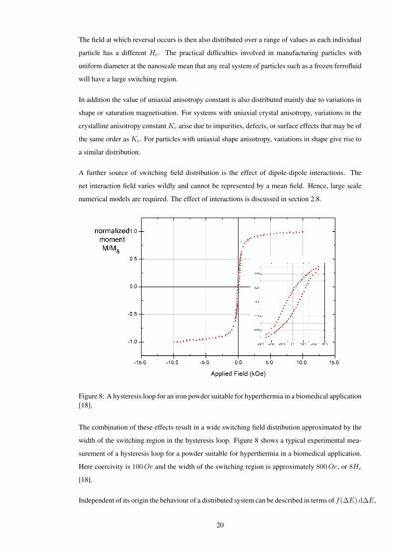
The field at which reversal occurs is then also distributed over a range of values as each individual
particle has a different Hc. The practical difficulties involved in manufacturing particles with
uniform diameter at the nanoscale mean that any real system of particles such as a frozen ferrofluid
will have a large switching region.
In addition the value of uniaxial anisotropy constant is also distributed mainly due to variations in
shape or saturation magnetisation. For systems with uniaxial crystal anisotropy, variations in the
crystalline anisotropy constant Kc arise due to impurities, defects, or surface effects that may be of
the same order as Kc. For particles with uniaxial shape anisotropy, variations in shape give rise to
a similar distribution.
A further source of switching field distribution is the effect of dipole-dipole interactions. The
net interaction field varies wildly and cannot be represented by a mean field. Hence, large scale
numerical models are required. The effect of interactions is discussed in section 2.8.
Figure 8: A hysteresis loop for an iron powder suitable for hyperthermia in a biomedical application[18].
The combination of these effects result in a wide switching field distribution approximated by the
width of the switching region in the hysteresis loop. Figure 8 shows a typical experimental mea-
surement of a hysteresis loop for a powder suitable for hyperthermia in a biomedical application.
Here coercivity is 100Oe and the width of the switching region is approximately 800Oe, or 8Hc
[18].
Independent of its origin the behaviour of a distributed system can be described in terms of f(∆E) d∆E,
20

a function of the energy barriers in the particles. f(∆E) d∆E gives the probability of finding a
barrier between E and E + ∆E. The barrier will be lowered by the application of a field. Such a
distribution must be normalise to unity as below.
∞∫0
f(∆E) d(∆E) = 1 (23)
The remanence in a system depends on the degree of alignment of the easy axes and lies between
0.5 and 1.0 in the absence of thermal activation. The ratio Mr/Ms is usually called the loop
squareness. It is limited by non-alignment of the easy axes that gives rise to a reversible component
of the magnetisation.Mr
Ms= Mmax
r
∫f(∆E) d(∆E) (24)
The coercivity is a much more complex factor since it requires a balance of regions magnetised in
different directions, including any form of reversible magnetisation [19].
2.6 Thermal Activation
The internal energies of a system of particles at T 6= 0 follow the Boltzmann distribution, and the
moment of a single domain particle at T 6= 0 is subject to thermal fluctuations. It follows then that
in an originally saturated system placed in zero field and where the energy barrier to reversal is
∆E = KV (1−H/HK)2, some particles may reverse instantaneously and some may reverse after
a time t due to the influence of thermal fluctuations.
Figure 9: A plot of equation 25 using H = 0 with K and T constant. The Neel relaxation timeranges from nanoseconds to centuries depending on the volume of the particle.
21
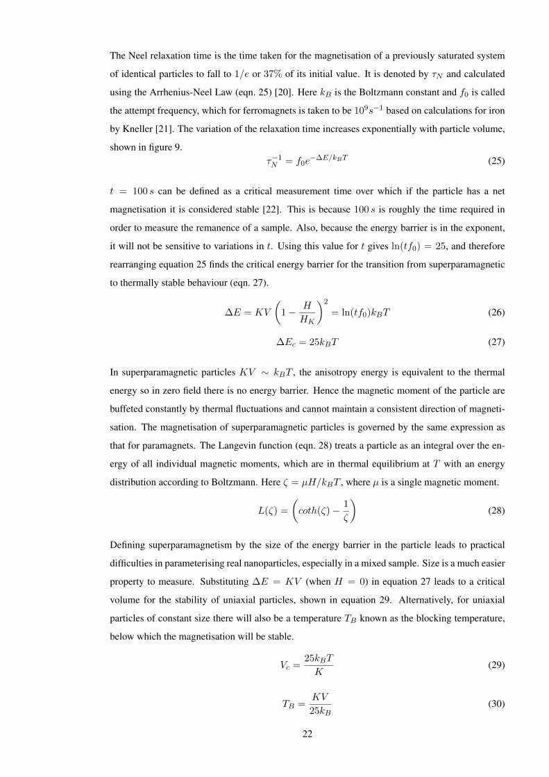
The Neel relaxation time is the time taken for the magnetisation of a previously saturated system
of identical particles to fall to 1/e or 37% of its initial value. It is denoted by τN and calculated
using the Arrhenius-Neel Law (eqn. 25) [20]. Here kB is the Boltzmann constant and f0 is called
the attempt frequency, which for ferromagnets is taken to be 109s−1 based on calculations for iron
by Kneller [21]. The variation of the relaxation time increases exponentially with particle volume,
shown in figure 9.τ−1N = f0e
−∆E/kBT (25)
t = 100 s can be defined as a critical measurement time over which if the particle has a net
magnetisation it is considered stable [22]. This is because 100 s is roughly the time required in
order to measure the remanence of a sample. Also, because the energy barrier is in the exponent,
it will not be sensitive to variations in t. Using this value for t gives ln(tf0) = 25, and therefore
rearranging equation 25 finds the critical energy barrier for the transition from superparamagnetic
to thermally stable behaviour (eqn. 27).
∆E = KV
(1− H
HK
)2
= ln(tf0)kBT (26)
∆Ec = 25kBT (27)
In superparamagnetic particles KV ∼ kBT , the anisotropy energy is equivalent to the thermal
energy so in zero field there is no energy barrier. Hence the magnetic moment of the particle are
buffeted constantly by thermal fluctuations and cannot maintain a consistent direction of magneti-
sation. The magnetisation of superparamagnetic particles is governed by the same expression as
that for paramagnets. The Langevin function (eqn. 28) treats a particle as an integral over the en-
ergy of all individual magnetic moments, which are in thermal equilibrium at T with an energy
distribution according to Boltzmann. Here ζ = µH/kBT , where µ is a single magnetic moment.
L(ζ) =
(coth(ζ)− 1
ζ
)(28)
Defining superparamagnetism by the size of the energy barrier in the particle leads to practical
difficulties in parameterising real nanoparticles, especially in a mixed sample. Size is a much easier
property to measure. Substituting ∆E = KV (when H = 0) in equation 27 leads to a critical
volume for the stability of uniaxial particles, shown in equation 29. Alternatively, for uniaxial
particles of constant size there will also be a temperature TB known as the blocking temperature,
below which the magnetisation will be stable.
Vc =25kBT
K(29)
TB =KV
25kB(30)
22

It has been shown that the energy barrier is modified by an applied field, hence the distribution of
energy barriers is a complex function. Figure 10 shows the shape of the distribution function and
the regions of distinct behaviour which contribute to it. Equation 31 describes the three regions as
integrals over f(∆E) [19].
Figure 10: The distribution of energy barriers can be divided into three sections which categorisethe types of behaviour.
∆Ec(0)∫0
L(ζ)f(∆E) d(∆E) +
∆EcHc∫∆Ec(0)
f(∆E) d(∆E) =
∞∫∆Ec(Hc)
f(∆E) d(∆E) (31)
Each value of ∆E has an exponential decay. Time dependence can now be seen to occur at the
value of ∆Ec that is active, but many discreet values of ∆E will be active around ∆Ec. This sum
of exponentials lead to a variation of M which is linear in ln(t) (eqn. 33) [23].
M(t) = M(0)− S ln(t) (32)
dM
d ln(t)= −S(H) (33)
Since there are a different number of particles at varying values of ∆E, the rate of logarithmic
decay S varies with field. It passes through a maximum at the peak of the distribution at a field
generally close to Hc.
23

2.7 Frequency Dependent Effects
Hysteresis Losses
The time dependence of the magnetisation when an alternating field is applied leads to a frequency
dependence of hysteresis loss. From the Sharrock law (eqn. 34) [24] it is possible to find an analytic
solution for the coercive field Hc. The Sharrock law makes some simplifications and is only valid
when the particles are not interacting and all the easy axes are aligned with the applied field.
Hc(t) = HK
(1−
√kBT
KVln
[tf0
0.693
])(34)
As the Sharrock law also assumes a static external field, in order to investigate frequency dependent
effects it has first to be modified for an alternating field. It has been shown previously that the
stepped field and swept field processes are related by the expression in equation 35 [25], where
teff is the effective time to be used for t in equation 34 and R = dH/dt is the field sweep-rate.
It follows that coercivity must be dependent on the rate of sweep of the field, which is given in
equation 36 [26]. Here hc = Hc/HK .
teff =kBT
KV
R−1HK
2(1−Hc/HK)(35)
Hc(R) = HK
(1−
√kBT
KVln
[kBT
KV
f0HK
2(1− hc)1
R
])(36)
Figure 11: Coercivity plotted against sweep-rate for metal particle tape shows the increase in Hc
as frequency increases [27].
24

Figure 11 uses a logscale for the measurement times used to find the coercivity range over 16
decades [27]. The scale is normalised to R0, the initial sweep-rate. For low sweep-rates the
coercivity increases linearly with ln(R/R0), but this trend does not continue as R increases. This
is because for high sweep-rate f0 is a limiting factor as t→ 10−9.
The remanence and the coercivity are both increased at high sweep-rate, increasing loop square-
ness. Therefore the hysteresis losses are proportional to the square of the frequency. The frequency
of an alternating applied field is therefore a critical parameter in controlling the amount of heat pro-
duced from hysteresis losses, as shown in figure 12. For higher frequency sweeps of the applied
field, a greater proportion of the larger superparamagnetic particles have a relaxation time longer
than the time taken for each sweep of the loop. The loops for these higher frequencies are then
wider as more particles contribute to the hysteresis losses by exhibiting thermally stable behaviour.
Figure 12: Calculated curves for 7.5nm iron particles showing the expansion of the loops at highfrequencies, where a greater proportion of the particles exhibit hysteresis.
Other Losses
Particles in a fluid can rotate physically to align their moments with an applied field, this also
releases energy as heat. Whether or not rotation occurs depends on the size of the particles, V , and
the temperature T and viscosity η of the fluid in which they are dispersed. The minimum size at
which particles can undergo Brownian rotation is given by the Shliomis diameter (eqn. 37) [28].
25

DS =3
√24kBT
πK(37)
The Brownian rotation of the particles has a characteristic relaxation time, τB , given in equation 38.
The radius rh is the hydrodynamic radius of the particle, which is often larger than the radius of the
magnetic volume. These losses occur at fields low enough to allow the particles to physically rotate
before the Neel relaxation causes the magnetisation of the particle to flip. The two relaxation times
combine to give an effective time, τeff, where usually one mechanism is dominant (eqn. 39) [29].
τB =4π r3
hη
kBT(38)
τeff =τNτBτN + τB
(39)
Particles suspended in a colloidal ferrofluid have been shown to have greatly reduced heating when
Brownian relaxation is prevented [30]. When injected into a tumour it is reasonable to suppose
that the ability of the particles to move freely will be reduced by sticking to or possibly entering
the cells. The model used in this experiment treats the particles as frozen in position, therefore
Brownian losses are unable to contribute to the heating and are not considered.
The electrical conductivity of the particles induces eddy currents at the surface of the particle when
a changing field is applied. Eddy currents produce heat due to the resistance of the material, but
they also work to limit the penetration of the field into the particle, resulting in lower hysteresis
and susceptibility losses. Fortunately eddy currents have been shown to be negligible for small
particles (less than 100 nm in diameter) if the frequency of the the alternating field is also less than
10GHz [31]. At very high field strengths eddy currents can be generated in the human body itself,
causing non-specific heating in healthy areas that are not intended to be damaged. The product of
the maximum field and the frequency must be Hmaxf < 6.10 × 10⁶Oes−1, and the frequency
f < 1.2MHz, in order to prevent inductive heating of the surrounding tissues in the patient or
stimulation of nerves or cardiac muscles, which are both painful and dangerous [32].
Susceptibility, χ is a measure of how responsive a material is to an applied field, it has real and
imaginary components χ′ and χ′′ respectively. The imaginary component of the susceptibility is
equivalent to the energy released as heat. When a particle is subject to an alternating external
field susceptibility losses occur because the moments in an alternating field oscillate in order to
stay aligned with the field. Susceptibility losses occur at all field strengths, and are proportional
to the frequency. At high frequencies the moments lag behind the actual direction of the field
because they are unable to rotate fast enough to keep up. This causes a loss peak in χ′′ and the heat
produced, as shown in figure 13 [33].
26

Figure 13: A modelled curve; the maximum possible imaginary component χ′′ is half that of thereal component χ′. Here ω = 2πf and the curves are normalised to the maximum frequency [33].
2.8 Interaction Effects
Two types of interaction affect particulate or granular systems. The first is the dipole-dipole field
which is demagnetising overall but at close separation can be magnetising. The second is the
exchange interaction, which is strongly magnetising but has short range and is very sensitive to
the distance between moments. The exchange interaction dominates in systems such as thin films,
where grains are close packed and have ∼ 100% concentration. In general dipolar interactions
reduce the overall remanence of the sample. Hc has complex variation but broadly is reduced
according to equation 40, where ε is the packing fraction and is between 0 and 1 [34].
Hc(ε) = Hc(0)(1− ε) (40)
In the types of powder systems used for hyperthermia the packing fraction is very low, such that
the concentration of iron is between 5 − 10mg/ml [32]. Hence exchange interactions can be
discounted. In principal dipolar coupling will also be negligible but particle aggregation gives
rise to local concentrations where the effects will be significant. Therefore interactions can have
noticeable effects on the parameters of the hysteresis loops produced by fine particle systems. It
has been shown that interactions lead to a reduction in the saturation remanence [35], but the effect
on coercivity is more complex.
The original Sharrock law neglects interactions but can be modified to take account of the dipole
27

field by calculating effective terms for HK and KV . Using the modification given in equation 35
for a swept field and fitting to calculations of Hc for 3-D randomly distributed systems leads to the
following expression for an effective energy barrier [36]:
∆Eeff = (KV )eff(
1− H
HeffK
)2
(41)
1400
1600
1800
2000
2200
2400
2600
2800
3000
3200
0.05 0.1 0.15 0.2 0.25 0.3 0.35 0.4
HK
eff
Packing Fraction
20 nm15 nm10 nm7.5 nm
Figure 14: Effective HK is reduced at higher packing densities as a result of interaction effectsfrom surrounding particles, the effect is more pronounced for smaller particles.
Figure 14 shows that the value of the fitted parameter HeffK decreases for higher packing fractions,
where each particle will be subject to interactions with an increased number of neighbouring par-
ticles. However for systems of small mean particle diameter, ie with a significant proportion of
superparamagnetic particles, the reduction of HeffK is not the dominant effect. For these systems,
interactions have been shown to increase the coercivity at low frequencies [36].
Typical concentrations of magnetic material in fluids used in clinical trials are low, containing
approximately 100mgFe/ml [14]. Assuming the nanoparticles are made up of pure magnetite
this concentration equates to a packing fraction in the liquid of about 0.016. However, with the
improvement of targeting techniques it is likely that the particles can be concentrated in the tumour
tissue resulting in more nanoparticles perml than in the fluid, and consequently more particles will
contribute to produce a greater heating effect.
28

3 MAGNETIC HYPERTHERMIA
3.1 Basis of Magnetic Heating
As discussed in section 2.7 there are 4 mechanisms of heating in magnetic particles; Brownian ro-
tation, eddy current heating, susceptibility loss, and hysteresis loss. The mechanism which occurs
is dependent on the particle size V , but it is uncertain which mechanism is typically characteristic
of any particular size. As detailed earlier both hysteresis loss and Brownian rotation have critical
sizes that can be calculated and below which these mechanisms do not act. Eddy current heating
only occurs in particles larger than 100nm for frequencies below the GHz range [31]. In any
system where V is distributed it is likely that more than one mechanism occurs in any one sample.
The type of heating is also dependent on the environment in which the sample is located. For exam-
ple, a small particle encased in a polymer sphere will be unable to physically rotate thus removing
any component of heat produced via Brownian motion. Whereas for a system of aggregated par-
ticles the relevant hydrodynamic radius will be that of the cluster, consequently particles smaller
than the Shliomis diameter may be able to physically rotate [37].
Recently there has been both experimental and theoretical research looking into the contribution
of each mechanism to the heating of magnetic nanoparticles, as well as the effect of particle size
and size distribution of samples on the heating contribution of each mechanism [29] [38] [39] [40].
Irrespective of the mechanism, there are many reports of work undertaken to measure the total
heating effect in different systems [41] .
Figure 15: Measured heating curves for systems with varying mean diameter [18].
29

Figure 15 compares experimental data for the rate of heating of three systems with differing median
particle diameters subject to the same applied field strength and frequency [18]. It is clear that for
the system of small particles very little heating occurs as almost all particles are below the critical
sizes. However, for the two larger systems the initial rate of heating is larger for the larger particles
and after approximately 3 minutes reduces to become almost equal to the heating rate of the middle
system, as the curves become more parallel.
This suggests the same mechanism is dominant in both larger systems at this point, but the larger
system is also affected by a second heating mechanism at the initial time. It is believed that the
initial heating rate of the green curve is due to susceptibility losses, which are complex as the
particles are both multidomain and aggregated. The dominant mechanism for the red curve and
after a finite time for the green curve is linear, and this is believed to be due to the Brownian
rotation of the aggregate because for particles above the Shliomis diameter in a liquid environment
Brownian losses dominate [42].
When considering a system of aggregate particles, simple analytical models are insufficient to
accurately describe the behaviour of the sample. For realistic solutions a numerical integration is
necessary over all the particles in the system that considers how each particle is affected by its
position relative to all the other particles with which it is interacting. Rosensweig [43] has derived
a frequency dependent expression for the total power loss per unit volume of magnetic material
and implemented it in a theoretical model of some ferrofluid systems.
P = fEH = πµ0χ′′fH2
max (42)
0
0.2
0.4
0.6
0.8
1
0 1 2 3 4 5
No
rma
lise
d χ
Frequency [kHz]
real component
imaginary component
Figure 16: Real and imaginary components of the complex susceptibility for a system of particleswith no size distribution, calculated using equations 43 and 44
30

Recall that χ′′ is the imaginary component of the susceptibility and is relative to the susceptibility
loss heating. Figure 16 shows the frequency dependence of the real and imaginary components of
the complex susceptibility χ for a system of particles with uniform size. The curves are normalised
to the equilibrium susceptibility χ0, on which χ′ and χ′′ depend as defined below. χ0 itself is
variable with applied magnetic field.
χ =′ χ01
1 + (2πfτeff)2(43)
χ′′ = χ02πf
1 + (2πfτeff)2(44)
Here τeff is the combined relaxation time of Neel and Brown given above in equation 39, maximum
heating occurs when the Brown relaxation dominates in this term. When χ′′ is substituted in
equation 42 above an analytically solvable expression for the power dissipated in one second by
susceptibility and Brownian losses is found.
P = πµ0χ0fH2max
2πfτeff
1 + (2πfτeff)2(45)
In a comparison of heating rates of different materials (fig. 17) the two ‘softest’ materials as
characterised by their relatively low anisotropies, magnetite (Fe3O4) and maghemite (γ-Fe2O3),
produced peak heating rates over a third higher than cobalt ferrite and over twice as high as barium
ferrite. The diameters of the particle systems which produced these high heating rate were also sig-
nificantly larger than the diameters corresponding to the CoO·Fe2O3 and BaO·6Fe2O3 peaks. The
optimum diameters were approximately 7nm and 8nm for barium and cobalt ferrite respectively.
The peak for magnetite was at ∼ 14nm and for maghemite ∼ 20nm; below these diameters the
particles would tend to become superparamagnetic, and so the amount of heating would become
minimal.
The rate of heating in figure 17 is related to the anisotropy strength of each material and the de-
pendence of Vc on K in equation 29. Even though the minimum particle sizes for these materials
to produce any heat are larger than particle sizes in a stable colloid, other requirements for some
clinical uses of nanoparticles will mean that they will be encapsulated in a polymer shell limiting
aggregation.
The systems were modelled as monodisperse particles, i.e., with standard deviation of particle size
σD = 0. The effect of a lognormal distribution of size dispersion was introduced in calculations for
magnetite and shown to have a significantly detrimental effect on the heating rate. The peak heating
rate was reduced from∼ 700K/s to∼ 400K/s when the standard deviation of size distribution σ
was increased from 0 to 0.05. However, an incredibly fast heating rate such as this is inappropriate
for clinical application in any case. If the heating is not carefully controlled there is a severe risk
to the patient of burns and damage to healthy tissues.
31

Figure 17: Curves showing heating rate against particle radius for 1. BaO·Fe2O3, 2. CoO·Fe2O3,3. Fe3O4, and 4. γ-Fe2O3 [43].
3.2 Materials and Equipment
In order to produce significant heat output whilst limiting the strength and frequency of the field
it would be preferable to use one of the more strongly magnetising materials such as cobalt. Un-
fortunately many magnetic materials are highly toxic to humans. This problem is compounded by
the reactions of nanoscale particles in the human body, which are not fully understood. In fact it
has been found that even usually inert materials such as gold can have detrimental effects when
introduced into the body for certain sizes of nanoparticle [44].
Currently the only magnetic material that has been found to be biocompatible and approved for use
in humans is magnetite. The enhanced toxicity of other nanoparticles is for the moment unlikely to
be overcome. However it is possible that in the future the use of more strongly magnetic materials
coated in an inert shell will be an option for hyperthermia treatment [45]. There is research ongoing
into the effects of core-shell interactions on the magnetic properties of nanoparticles [46].
In the early days of nanoparticle manufacturing for use in ceramics and powder metallurgy in-
dustries many particles were produced by grinding large specimens into finer and finer powder,
a process known as milling [47]. Now there are many methods of chemically building nanopar-
ticles through deposition or nucleation, allowing the characteristics to be tailored to specific re-
quirements. These include small particles diameters with very narrow size distributions. Magnetic
nanoparticles have also been combined with other materials producing systems with applications in
32

sensing, biocatalysis, targeted infection, magnetic resonance imaging, and drug delivery [48]. Fig-
ure 18 shows an image taken with a transmission electron microscope of a single layer of γ-Fe3O4
particles in a ferrofluid with very uniform diameters of ∼ 11nm [49].
Figure 18: TEM image of 2-D assembly of 11nm diameter γ-Fe2O3 nanoparticles with narrowsize distribution [49].
Nanoparticles can be manufactured to the necessary standards for use in clinical trials, but a method
of field generation is also required. For small scale usage commercial bench-top hyperthermia
devices are available which have frequency ranges of 50 kHz to 1.2MHz with field strengths
up to 250Oe [50]. These systems can be used in particular to insert plasmids or other biological
material into cells via a magnetic nanoparticle carrier, which is much less harmful to the cell than
injection or other methods.
This sort of equipment is unsuitable for use in humans on a clinical scale. Patients may require
treatment on organs located deep within the body, such as the liver, and to generate a homogeneous
field over a large area requires a more powerful field generator. Alternative methods of heating
have been trialed such as radiofrequency waves, microwaves, and ultrasound, but all of these have
the limitation of being unable to target the tumour sites specifically and also suffer inhomogeneous
temperature distribution due to difficulties penetrating uniformly through body tissues.
Clinical studies of magnetic hyperthermia were begun by Jordan et al. [10] at Charite University
Hospital in Berlin in 2000. The alternating field generator machine designed and built there for
treatment of humans is shown in figure 19. It has a ferrite core to boost the field strength output
and is capable of a field frequency of 100 kHz for field strengths up to 225Oe over a vertical
treatment space of 30− 45 cm in which the patient must lie.
33

Figure 19: The MAG-300F alternating field generator at Charite University Hospital, Berlin [12].
Since then, many trials have investigated the suitability of magnetic nanoparticles for treating par-
ticular types of cancers using in vitro and animal studies. Studies of the amount of heating produced
by differently manufactured nanoparticles and the best coatings for stability in vivo have been un-
dertaken in rats. More recently, phase I and II clinical trials have been conducted in humans and
the effectiveness of magnetic hyperthermia as both a stand-alone treatment and in conjunction with
surgery, radiotherapy, and chemotherapy has been evaluated [51].
3.3 Applications
Studies have shown that rats are a good model for the evolution of malignant glioma in humans.
This is a type of aggressive brain tumour which is currently untreatable [52]. A study of magnetic
hyperthermia in rats with glioma, using coated magnetite particles in field strengths up to 225Oe
at 100 kHz produced temperatures inside the tumours of 43− 47o which could be finely adjusted
by tuning the field strength. These temperatures caused areas of necrosis in the tumours and life
expectancy of the rats increased up to 4.5 times that of the control group for the highest tempera-
tures [11]. For cases in humans where no other treatment method is viable, or has failed it may be
possible to use hyperthermia as a palliative treatment, extending life expectancy or the quality of
life without causing the detrimental side-effects associated with chemotherapy.
34

As an isolated treatment magnetic hyperthermia cannot guarantee complete destruction of all tu-
mour cells due to the difficulties involved in ensuring uniform particle, and consequently tempera-
ture, distribution throughout an irregularly shaped tumour. As a result of areas with lower particle
concentration there may be cool spots within the tumour which can survive the treatment and be
undamaged so that they can continue to replicate. The nature of cancer being uncontrolled cell
division this will then cause a recurrence of the tumour. However in the case of slow growing and
most importantly benign tumours such as those which cause enlargement of the prostate gland,
magnetic hyperthermia has been used as an alternative to repeated surgical intervention.
Figure 20: CT scan of a cancerous prostate gland before, immediately after, and 6 weeks aftermagnetic hyperthermia therapy. Image reprinted from [12].
The first report on clinical application of interstitial hyperthermia using magnetic nanoparticles
in the treatment of human cancer was published in 2005 [12]. Figure 20 shows a computerised
tomography image from that paper of a prostate gland containing a benign tumour before and after
magnetic hyperthermia treatment. The magnetite particles remained stable in the prostate for the
full six weeks of treatment and did not require subsequent ‘top-up’ injections.
Hyperthermia has also been shown to improve the clinical outcome of patients simultaneously un-
dergoing radiation therapy [3]. If used correctly, hyperthermia not only causes an additive effect,
but can work synergistically with the standard treatment. The optimum timeframe is thought to in-
volve radiation first followed 3−4 hours later by hyperthermia [53]. For this particular application,
temperatures of 41.5− 43oC, referred to as ‘mild temperature hyperthermia’ are employed. These
temperatures do not kill most types of cell directly but DNA repair is often inhibited for a short
time after the treatment which prevents cells previously damaged by radiation from successfully
recovering and replicating. Another factor in the improved response is the sensitisation of cells
that are normally resistant to radiation, such as those in a low pH environment or in the process
of replicating. The first of these conditions is very common inside tumours due to poor circula-
tory systems caused by unregulated growth which is itself due to the cancerous cells continually
replicating.
35

3.4 Future Developments
Future developments in hyperthermia for the treatment of malignant diseases and other tumours
are likely to be in the areas of improving functionalisation of nanoparticles to better target only
certain types of cell and only cancerous cells of that type. Research into this is being undertaken
by the MULTIFUN project [54], which has brought together experts in biomedicine, oncology, and
chemistry from research groups, hospitals, and companies that manufacture nanoparticles. The
goal of MULTIFUN is to develop magnetic nanoparticles designed for ‘theragnostics’: combining
diagnosis and imaging of tumours with multiple methods of targeted therapy.
This involves attaching biological molecules to nanoparticles which cause them to accumulate in
tumour tissue. Once there the magnetic properties allow the particles to perform as contrast agents
to pinpoint tumours in MRI imaging. If the particles are injected intravenously this method could
potentially highlight secondary tumours that have spread to other parts of the body while they are
still small. When a tumour is confirmed the dose of functionalised nanoparticles can be increased
as necessary. The application of an alternating magnetic field will then apply targeted heating
which can simultaneously sensitise the cells and trigger the release and activation of anti-cancer
drugs. Figure 21 shows the three separate mechanisms that can be achieved with functionalised
nanoparticles.
Figure 21: The three applications of functionalised magnetic nanoparticles being researched by theMULTIFUN project [54]
36

3.5 Objectives of this Work
Clinical trials on both rats and humans have demonstrated hyperthermia therapy as proof of concept
for particular forms of cancer. However, due to the wide variations in how quickly the same type of
cancer grows and spreads, and the differing degrees of response to any treatment in different people,
large sample sizes are required to accurately assess the effectiveness of the treatments. As a result
of this experiments on animals tend to only compare 2 or 3 sets of parameters alongside a control
group. Theoretical studies can help focus practical experiments by exploring a wide selection of
magnetic materials, as well as changing the parameters of the nanoparticles and the applied field, to
find biologically viable combinations of these which produce the greatest heat output for the most
economical input conditions, without the expense and bureaucracy of performing clinical trials.
The purpose of this project was to investigate the optimum parameters for generating the maximum
amount heat from hysteresis losses in biologically compatible nanoparticles. To this effect the
behaviour of a variety of systems of randomly dispersed nanoparticles made of iron-based magnetic
materials were simulated for a number of different particle diameters and packing fractions while
the systems were subjected to an alternating field over a range frequencies and maximum field
strengths.
37

4 SOFTWARE METHODS AND DEVELOPMENT
4.1 Principle of the Model
The system considered in this experiment is a sample represented by a cubic cell of interacting
single domain particles with periodic boundary conditions. A lognormal distribution characterises
both the diameter and the anisotropy constants of the particles, which have standard deviations of
0.1. The anisotropy easy axes are also distributed randomly in three dimensions, as would be the
case for a solidified colloidal ferrofluid. The simulation is supposed to be useful to compare with
experiments and medical trials, consequently the temperature used throughout is body temperature,
310K.
The highest percentage of magnetic material contained in a unit of colloidal ferrofluid is ∼ 15%,
since if further concentration is attempted the particles will tend to aggregate [42]. The concentra-
tions of magnetic material that can be safely injected into a human being are much lower than the
technical limits of ferrofluid density. This is especially true if the substance is intended to circulate
in the bloodstream rather than be injected directly into the tumour site. Despite the low densities
at injection, the state of the system within the tumour may well be much higher as particles accu-
mulate at the targeted site. Consequently the densities investigated here are between 5% and 40%
to account for the possibility of non-colloidal states in vivo.
The assembly of nanoparticles is modelled with a kinetic Monte-Carlo algorithm which takes into
account the behaviour of both superparamagnetic and thermally stable particles. For the mean
diameters considered in this case (5-20nm) there will be a non zero fraction of superparamagnetic
particles [55].
This model makes use of the Mersenne Twister [56], a random number generator well suited to
Monte-Carlo algorithms as they require a very large sequence of unique random numbers. The
Mersenne Twister has a period of 219937 − 1 and passes many tests for statistical randomness.
Two mechanisms are used to calculated the probability of magnetic reversal Pr, depending on
whether the particle is classed as superparamagnetic or thermally stable. Thermally stable particles
defined by the parameter KV > kBT ln(tf0) are treated as Stoner-Wohlfarth particles with two
energy minima. In order to account for thermally activated switching a probability of switching
between minima proportional to the magnitude of the energy barrier is included. Otherwise, for
particles where ∆E < 3kBT the energy barrier is so small that the two-state approximation is
invalid. The direction of the moment must be considered able to point in any direction and the
probability of it being found in a particular direction is derived from the Boltzmann distribution.
38

4.2 Initialisation of the Particle Array
Figure 22 shows an example of the initialised particle system. It is impossible to produce this
arrangement through random assignment of particle co-ordinates at high packing densities because
the probability of particles overlapping becomes too high. The method used here is based on
creating a system initially of low packing fraction and then shrinking to the required concentration.
The size of the cubic cell is initially defined as having a length of 4 3√N D, where D is the median
diameter and N is the number of particles in the simulation. This gives a low initial density and
allows plenty of space for the particles to be placed in at random. The particles are assigned radii
according to a lognormal distribution with σ = 0.1, and their random co-ordinates in the cubic cell
are generated.
Figure 22: A visual representation of the arrangement of 1000 particles generated by the systeminitialisation code at 10% packing fraction produced using Povray, an image rendering program.
A neighbour list is drawn up which keeps track of where each particle is located in an array of
sub-cells. This is to cut down on computational time when checking whether particles are touching
or overlapping after they are moved. Each particle is checked only against the particles in the same
and immediately neighbouring sub-cells.
The system is then checked for particles occupying the same space and if necessary expanded to
remove overlaps. So that the system can be shrunk to the required density quickly the particles
are encouraged to move apart by application of a repulsive potential. The energy Ei is quartic
with respect to the magnitude of separation rij between the central co-ordinates of particle i and
surrounding particles j.
Ei =∑j 6=i
1000×(dmrij
)4
(46)
39

A Monte-Carlo algorithm moves each particle a small distance and compares the new energy to the
old ∆Ei = Enew,i−Ei. The new position of the particle is accepted if the particle has moved away
from its neighbours ∆Ei < 0. It is also accepted with a probability that decreases as ∆Ei increases
by comparison to a uniformly generated random number, expressed as exp (−∆Ei) < [0, 1[. Thus
as the particles attempt to move closer together the potential energy is increased and the move is
less likely to occur. As the moves are accepted the neighbour list is updated as necessary. This is
repeated 50 times for each particle.
The smallest separation between any two particles is then calculated and the system is shrunk until
those particles are almost touching. The Monte Carlo process is then repeated and the system
shrunk again until the desired packing density is reached. A final run through the Monte Carlo
process equilibrates the system. This algorithm efficiently produces random configurations for
particle densities of up to 25% of the cubic volume for 8000 particles. The code which produces
the initial configuration is included in the appendix.
4.3 Demagnetising the System
The initial state of the system is random, and so it is likely that the internal energy will not be
minimised. When the hysteresis loop is generated the field strength begins at zero, so it is neces-
sary to produce a realistic demagnetised state [57]. This is especially important when only minor
hysteresis loops are generated, as in this case the net magnetisation of the system is not maximised
at any point. Without initially demagnetising the system, the simulation could begin at zero field
in a higher energy state than the maximum applied field would be able to produce in reality.
-1
-0.5
0
0.5
1
0 1000 2000 3000 4000 5000 6000
-5
0
5
Ma
gn
etis
ati
on
(M
/Ms)
Ap
pli
ed F
ield
Str
eng
th [
kO
e]
time [s]
M
H
Figure 23: Curves showing the application of an alternating applied field (blue curve, right axis)which reduces over time drives the net magnetisation of 20nm iron particles to zero.
40

To demagnetise the system a field of 5000Oe is initially applied. This is strong enough to almost
magnetise a system of magnetite or iron particles. The field is slowly reversed, to allow the mag-
netisation of the system to follow closely and the maximum field strength is reduced at each cycle.
As is shown in figure 23, after many cycles the system is left in a demagnetised state when the
applied field and net magnetisation are reduced to zero.
4.4 Interaction Field
The dipolar interactions from surrounding particles results in a dipolar field which acts on each
particle. This must be calculated and added to the external field to discover the total field acting on
each particle. In equation 47 the local field Hloc is the vector sum of the dipolar interaction fields
produced by the moments of surrounding particles µj on each particle i and the applied field Happ.
Hloc =∑j 6=i
[3(µj .rij)
r5ij
− µjr3ij
]+Happ (47)
Here the 1/r3 dependence leads to the contribution from each particle to the dipolar field dimin-
ishing rapidly as the separation distance between two particles, rij increases. Consequently, to
conserve computational time the summation was calculated for all j within range to up to a cut-off
radius r < rmax. A mean-field approximation for a spherical sample shape was used to calculate
the contributions from particles outside this range. For these calculations rmax was set to be five
times the median diameter of the particles.
4.5 Hysteresis Loop Calculation
Consider the method implemented on superparamagnetic particles. The moments of these particles
exist in a thermal equilibrium therefore must be characterised by polar co-ordinates θ and φ. Con-
sequently the energy of each particle i can be defined as a function of these angles where any angle
is possible, and the fieldE(θ, φ,Hloc). The direction of the moment is then distributed according to
Boltzmann statistics, with a probability for each state given by equation 48, where z is the partition
function, which is equal to the sum of all the possible states ensuring that the maximum value for
the probability Pi is 1.
Pi =1
ze−∆Ei/kBT (48)
z =∑i
e−∆Ei/kBT (49)
41

The reversal probability of superparamagnetic particles defined by ∆E < ln(tf0)kBT is calcu-
lated using the Metropolis algorithm [58]. The Metropolis algorithm works by producing a new
state for the particle with the moment at random values of θ and φ and calculating the energy dif-
ference with the previous state. If the new energy is lower than the original energy, i.e., ∆E < 0
the new position is accepted. If ∆E > 0 it is accepted with the probability defined in equation 50;
if exp(−∆E/kBT ) is lower than a uniformly generated random number between 0 and 1 to which
it is compared.
Pr = min(1, e−∆E/kBT ) (50)
Figure 24: A schematic of the moments in single domain particles. Superparamagnetic particlescan point in any direction, whereas thermally stable particles are restricted to two energy minima.
The difference between the allowed directions of the moments in superparamagnetic and thermally
stable particles is shown in figure 24. For thermally stable particles as defined by ∆E > ln(tf0)
the Metropolis algorithm is inefficient because the probability of the moment being found any-
where other than close to the energy minima is extremely small. It would therefore take a long
time to produce a realistic statistical distribution of moment probabilities. Consider instead then a
simulation algorithm based on the Stoner-Wohlfarth particle theory. In this theory, the total mag-
netic moment of a particle is described by µ which is the product of the particle volume V and the
saturation magnetisation Ms.
The energy of a single particle is given previously in equation 6 and produces two energy minima
denoted by E+ and E−, aligned parallel and antiparallel with the anisotropy field respectively, and
separated by an energy maximum E0. Note that these energy values are magnetic field dependent.
At certain threshold magnitudeHt one of the minima coincides withE0; eitherE+ = 0 orE− = 0
depending on whether HKcos(ψ) > 0 or < 0, respectively. It has been calculated [59] that the
threshold field is Ht = HKg(ψ), where HK = 2K/MS is the anisotropy field and
g(ψ) = (cos2/3 ψ + sin2/3 ψ)−3/2 (51)
42

Here ψ is the angle between K and H . Thus for field magnitudes H < Ht there are two stable
states and for H > Ht there is one unique state. Accordingly a Stoner-Wohlfarth particle shows
hysteresis when magnetisation M is plotted as a function of the field H . Thus switching of a
particle between the two states occurs whenever the magnitude of Hloc,i becomes equal to the
threshold field Ht,i.
So far this method is entirely deterministic, which is suitable for particles with ∆E >> ln(tf0)kBT .
However, although many particles have energy barriers large enough to be modelled as a two-state
system, they are also small enough to be influenced by thermal fluctuations.
Including the spontaneous reversal effect of thermal activation in the model requires probabilistic
expressions, hence probabilities P+,i(t) and P−,i(t) are assigned for a particle to be in its ‘+’ or
‘−’ state at a given time t, respectively. The normalisation condition gives P+,i(t) + P−,i(t) = 1
for all values of t and the time evolution of these probabilities is governed by the master equation:
dP+,i(t)
dt= −w+,i(t)P+,i(t) + w−,i(t)P−,i(t), (52)
Here w+,i and w−,i are transition rates for moment transitions from ‘+’ to ‘−’ and from ‘−’ to
‘+’, respectively, and are related to the Neel relaxation time τ−1N = w+,i + w−,i. The transition
rates are assumed to take the Arrhenius form:
w±,i = f0 exp (−∆E±,i/kBT ) (53)
The energy barriers are defined as ∆E±,i = E0,i −E±,i with E0,i, E±,i being the energies associ-
ated with the energy maximum and the two minima according to the discussion above. The smaller
of the two energy barriers can be calculated using by the numerical Pfeiffer approximation [59].
∆E(ψi, Hloc,i) = KiVi
[1−
Hloc,i
g(ψi)
]κ(ψi)
, (54)
Here g(ψi) is given by equation 51 and the exponent κ(ψi) = 0.86 + 1.14g(ψi). With these
definitions, equation 52 can be solved in a straightforward manner under the assumption of constant
external field H , which implies time independent rates w±,i, and
P±,i(t) = w∓,iτN (1− exp (−t/τN )) + P±,i(0) exp (−t/τN ) (55)
τN is the characteristic relaxation time associated with the particle i, and P±,i(0) are the initial
values for probabilities at time t = 0. For long times t→∞, and equation 55 leads to equilibrium
solutions where ∆E±,i = E0,i − E±,i.
43

P±,i(∞) = w∓,iτN =e−∆E∓,i
e−∆E+,i + e−∆E−,i=
e−E∓,i
e−E+,i + e−E−,i, (56)
Thus, according to equation 55, if a particle i is initially in the state ‘+’, for example, which implies
P−,i = 0 and P+,i = 1, the probability that this particle can be found in the ‘−’ state after the time
∆t is P−,i(∆t) = w+,iτN (1− exp (−∆t/τN )), and similarly for the opposite switching event
starting from the initial state P−,i = 1 and P+,i = 0. Thus, the condition for finding the particle
moment in the opposite state after time ∆t can be expressed by equation 57, where Pi(∞) is given
by equation 56 depending on the initial state.
Pi(t) = Pi(∞) (1− exp (−∆t/τN )) , (57)
Given the consideration above, we can formulate the computational algorithm to follow the time-
evolution of the magnetisation state as a sequence of the following rules:
1 Assuming external field is H at time t, increment the field to be H ′ = H + ∆H at time
t′ = t+ ∆t.
2 Pick a particle i and find ‘+’ and ‘−’ states by the energy minimisation of equation 6 when
subject to Hloc,i.
3 Calculate E0,i, E±,i, ∆E±,i from equation 54 and w±,i using equation 53.
4 Evaluate probability Pi(∆t) of switching during the time interval ∆t according to equa-
tion 57.
5 Generate a random number between 0 and 1 according to a uniform distribution and switch
the particle i if r > Pi(∆t), otherwise do nothing.
6 Update the local fields Hloc,j acting on neighbours of a particle i according to equation 47.
7 Go to step 2 and repeat steps 2-7 N times until all particles have been chosen.
8 Go to step 2 and repeat steps 2-8 Nmcs times, where Nmcs is the number of Monte-Carlo
steps. This is essential for averaging.
9 Set H = H ′ and t = t′. Return to step 1 and continue until a hysteresis loop is generated.
Thus the sequence of steps 1-8 defines the particle state evolution during the time interval δ t =
∆ t Nmcs, which can be thought of as the time interval during which the external field is in-
cremented by ∆H . This allows the definition of the external field rate as R = ∆H/δt =
∆H/(∆tNmcs).
44

4.6 Extracting information from the loops
To find the coercivity the hysteresis loop data was analysed and the equation describing the straight
line joining the first two points found either side of the zero axis was calculated. From this the
value of H at the point where that line crosses zero was determined. This finds the first time that
the magnetisation goes below zero and so for a hysteresis curve with lots of noise, such as one
describing a minor loop, this method will underestimate the true coercivity. However, when con-
sidering minor hysteresis loops the coercivity is not a particularly useful property, as the reduced
squareness of minor loops renders the estimation of the area given by the coercivity inaccurate.
To find the area of the loop the values of the magnetisation were increased, a shift of +1 ensures
the loop has only positive values for M/Ms. Treating the upper and lower curves separately the
difference in the area was found by numerical integration of each curve using the trapezoidal rule.
This method requires the integrand to be described by a sequence of equally spaced points. The
error is proportional to 1/n2, where n is the number of points used to evaluate each curve.
The energy lost as heat through one complete cycle of the field has been described as a function of
the hysteresis loop area previously in equation 1. However, as the field can alternate over a large
range of frequencies a more useful measure is the energy dissipated in a set amount of time, the
power:P = fMs
∫MdH (58)
-1
-0.8
-0.6
-0.4
-0.2
0
0.2
0.4
0.6
0.8
1
-3 -2 -1 0 1 2 3
Mag
net
isa
tion
(M
/Ms)
Applied Field Strength [kOe]
Hmax = 4990 Oe
Hmax = 1999 Oe
Hmax = 999 Oe
Figure 25: A comparison of hysteresis loops produced for different values of Hmax on an ironcomposite.
45

The integral goes from Hmax to −Hmax. The effect on the heat output of the range of the field
is shown in figure 25. Here the frequency used for the three loops is the same, but the maximum
applied field is only strong enough to fully magnetise the sample and complete the hysteresis
loop for the blue curve. Both the red and black curves form minor loops with correspondingly
lower values of Mr and Hc because the demagnetising dipolar field which is produced by the
unmagnetised fraction at Hmax = 1 kOe and Hmax = 2Oe is contributed to by 80% and 50% of
the particles in the sample respectively.
In summary a model has been developed to generate a system of interacting magnetic fine particles
and calculate the heating due to hysteresis when an alternating magnetic field is applied. This
allows the amount of hysteresis heating produced by different materials and system parameters to
be investigated, as well as the effects of dipolar interactions on the amount of hysteresis heating.
The model can also be used to calculate the frequency dependence of the hysteresis heating, leading
to a value of optimum frequency for heating a given system.
46

5 RESULTS
5.1 Properties of fine particle magnetic systems
The hysteresis losses generated by interacting fine-particle systems are governed by many compet-
ing factors which effect the shape of the hysteresis loop. Those due to the intrinsic properties of the
material are the anisotropy K and the saturation magnetisation Ms. The physical arrangement of
the system is defined by the median volume of the particles Vm which are distributed lognormally,
as well as the packing fraction ε. The characteristics of the applied field are the maximum value
Hmax and the sweeping-rateHrate or frequency f . The strength of interaction effects in the system
also influences the loop shape and is itself a complex combination of some of the factors already
mentioned, the equation for the interaction energy is:
Ei =~µ · ~µr3
=MsV1 ×MsV2cos(θ)
r3(59)
The strength of the interaction effect is dependent on three separate parameters. Firstly the square
of the saturation magnetisation Ms; as an example the saturation magnetisation of iron is approxi-
mately four times larger than that of magnetite, Ms = 1710 emu/cc and 470 emu/cc respectively.
This means that the strength of interactions in a system of iron particles compared to that between
magnetite particles is ∼ 16 times stronger. The size of the particles V1,2 will be calculated from
the lognormal distribution around the median particle diameter with a standard deviation σ = 0.1.
Finally, the distance between the particles r, which will be represented by the packing fraction ε as
an average for the whole system; r will decrease proportionally when packing fraction increases.
The interaction field is demagnetising overall and in places can be very strongly demagnetising, but
individual particles may exist in a position where demagnetising contributions from surrounding
particles cancel out, or in regions where the local field is magnetising. Since particle interactions
are a function of distance, it has been stated that systems with 0.05 packing fraction can be con-
sidered to behave as though they are non-interacting [36], however this is only the case when the
smallest r, the distance to the nearest particle is approximately the same for all particles, i.e., the
particles are arranged in a lattice structure. When particles are arranged randomly they tend to
clump together, consequently interactions inside clusters of particles are significant even when the
packing fractions are as low as 0.001 [42].
47

5.2 Interactions: Dependence on particle size
The proportion of superparamagnetic particles in a system is known to influence the width of the
hysteresis loop. When the median diameterDm is large, a greater proportion of the particles will be
thermally stable because the distribution ofDm is lognormal. It follows that for any particular field
sweeping-rate, hysteresis losses will increase non-linearly as the median particle size increases
until all particles contribute to the loss.
For this simulation a system of cobalt particles was chosen due to its high anisotropy which results
in a strong variation in the loops with grain size. Hexagonal close packed cobalt has a uniaxial
anisotropy constant of 4 × 10⁶ ergs/cc and Ms of 1400 emu/cc, and requires a field of at least
∼ 4 kOe to saturate it. A field strength of less than this would result in the formation of minor
loops, which would have other effects on the loop shape and area and make it more difficult to
observe the effect of particle size. Therefore the maximum field used was 5 kOe and the frequency
was 200Hz. The critical diameter for the transition to superparamagnetic behaviour can then be
calculated from the equation for critical volume Vc, equation 29.
Dc = 23
√3
4πVc (60)
From this equation, the critical diameter for the above parameters is found to be 6.7nm. Systems
with Dm between 5 and 20nm were investigated, and so it is expected that the 5nm system
exhibits primarily superparamagnetic behaviour although the tail of the lognormal distribution will
mean that some particles will be blocked. It is also expected that the 20nm system will contain
a majority of thermally stable particles. The systems investigated have a packing fraction of 0.05
and the temperature used was body temperature, 310K.
Hc = HK
[1−
(ln(tf0)kBT
KV
)1/2]
(61)
As shown in figure 26 the shape of the loop varies greatly when the median particle diameter is
close to the superparamagnetic limit. The coercivity increases from 30Oe for the system with
the smallest particles to 2.3 kOe for the larger particle system. The increase in coercivity as the
median diameter is increased from very close to the superparamagnetic limit is non-linear. From
equation 61 the size dependence of Hc can be seen to be proportional to 2√V , and the rate slows as
the maximum possible Hc is approached. As the particle diameter increases beyond the limiting
size for single domain behaviour they will break up into multiple domains and therefore total
volume is no longer a relevant size parameter.
48

−1
−0.8
−0.6
−0.4
−0.2
0
0.2
0.4
0.6
0.8
1
−4 −2 0 2 4
Ma
gn
etis
ati
on
Applied Field Strength [kOe]
K = 4x10⁶ ergs/cc
Ms = 1400 emu/cc
T = 310 K
ε = 0.05
5 nm
6.5 nm
7.5 nm
10 nm
20 nm
Figure 26: Hysteresis comparison of cobalt particles with different median diameters.
5.3 Interactions: Effects of packing fraction
From equation 59 it can be seen that the separation distance has an effect on the interaction strength.
The average separation is not measured, but it is known to decrease as packing fraction increases
since packing fraction is calculated from Vall particles divided by Vcubic cell, and the cubic cell was
‘shrunk’ over more iterations to generate systems with higher packing fractions. In systems where
the average separation distance is lower a greater number of particles will be included inside the
cut-off radius for calculating interactions, so the effect of interactions on the systems should be
enhanced by increasing the packing fraction.
For this simulation the parameters used are those for iron since it has the highest magnetisation,
thereby better illustrating the effect of interactions. The systems compared have packing fractions
of 0.05 and 0.2. The saturation magnetisation of iron is 1710 emu/cc, and the cubic anisotropy
constant is 4.2 × 10⁵ ergs/cc. The model assumes a uniaxial anisotropy, but for particles of iron
the crystalline anisotropy is not strong enough to overcome the effect of shape anisotropy due to the
nanoscale size of the particles. This changes the anisotropy from cubic to uniaxial and applies to
particles under 40nm in diameter [60] so the model is applicable in this case. The median diameter
of the system of particles was 20nm, temperature was 310K, the frequency of the alternating field
was 1 kHz and the maximum field strength was 1 kOe.
49

-1
-0.8
-0.6
-0.4
-0.2
0
0.2
0.4
0.6
0.8
1
-1000 -500 0 500 1000
Ma
gn
etis
ati
on
(M
/Ms)
Applied Field Strength [Oe]
K = 4.2x10⁵ ergs/cc
Ms = 1710 emu/cc
Dm = 20 nm
T = 310 K
ε = 0.05
ε = 0.2
Figure 27: Hysteresis loops of different densities of 20nm diameter iron particles with field alter-nating at a frequency of 1 kHz.
Figure 27 shows the hysteresis loops produced by this simulation. The interactions lower the
gradient of curve, which indicates overall they have a demagnetising effect and the interaction
field opposes the applied field. The area of the loop is reduced because generally both Hc and
Mr are reduced by interactions. However, the effects are often complex and an increase in Hc is
possible under certain circumstances. This is because the local micromagnetic configurations can
be magnetising or demagnetising depending on the magnetic history of the sample.
For this system the saturation field is increased significantly; the sample only reaches 60% satura-
tion in a 1 kOe field and therefore a minor loop forms which reduces the coercivity as well as the
remanence. For the 5% by volume sample a fully closed loop forms at a field less than 1 kOe but
for the 20% by volume sample the loop does not close and only 0.6Ms is achieved in a field of
1 kOe. This indicates that the effective overall dipolar field is demagnetising and of the same order
as the applied field.
On average the largest particles will be the last to be magnetised, and they will have the largest
interaction effect on other particles. Consequently, when the applied field is removed the large
particles which retained their opposing magnetisation will impose a significant demagnetising field
on the reversible particles and some of these are flipped, greatly reducing Mr. The result of this
simulation shows that interactions have very strong effect in systems of iron particles.
50

The same experiment as above was performed with the same system parameters, except with K
and Ms values representing magnetite. The cubic anisotropy of magnetite is 1 × 10⁵ ergs/cc and
saturation magnetisation is 470 emu/cc, again the anisotropy can be assumed to become uniaxial
for small particles. Interaction effects on magnetite systems should be less strong than those for
iron because the saturation magnetisation of magnetite is ∼ 4 times smaller. From equation 59 the
strength of interactions in magnetite are therefore ∼ 16 times weaker than in iron.
The effect of interactions in a system of magnetite particles is shown in figure 28, the saturation
field is increased as in iron but saturation is still achievable at fields lower than 1 kOe and a full
hysteresis loop is able to form, therefore a meaningful comparison can then be made between
the two systems of different packing fraction. The gradient of the curve is reduced by a much
lesser degree than for iron as a result of the lower saturation field. Interactions widen the loop by
increasing the coercivity from 36Oe to 66Oe, correspondingly increasing the area.
-1
-0.8
-0.6
-0.4
-0.2
0
0.2
0.4
0.6
0.8
1
-1000 -500 0 500 1000
Ma
gn
etis
ati
on
(M
/Ms)
Applied Field Strength [Oe]
K = 1x10⁵ ergs/cc
Ms = 470 emu/cc
Dm = 20 nm
T = 310 K
ε = 0.05
ε = 0.2
Figure 28: Hysteresis comparison of different densities of 20nm diameter magnetite particles withfield alternating at 1 kHz.
The remanent magnetisation is slightly lowered by interactions, this is because at the remanence
the only field acting on the particles is the dipolar interaction field, and at higher packing fractions
there are more neighbouring particles contributing to this field. When there are only a few neigh-
bouring particles some of them will couple to produce particle-pairs, these pairs reinforce each
others magnetisation. Whereas at high packing fractions there are large clusters of particles all
contributing to produce a stronger local field which gives rise to localised areas of zero net mag-
51

netisation by forming closed loop structures. Figure 29 shows a diagram of the arrangement of the
two types of structure.
(a) (b)
Figure 29: (a) Systems with low packing fraction arrangements result in the formation of particlepairs. (b) Particles in densely packed arrangements form closed loop structures.
5.4 Interactions: Dependence on Ms
In principle the hysteresis loss over one cycle of the alternating field is governed by the values ofHc
andMs, therefore an increase in theMs should result in a greater heating effect. In order to confirm
this the hysteresis loops of two otherwise identical systems with differing saturation magnetisations
have been compared. An anisotropy of 2 × 10³ ergs/cc was chosen, which is a typical value
for a soft magnetic material such as nickel-iron. The Ms values chosen were 1910 emu/cc and
860 emu/cc, these are representative of FeCo and NiFe respectively [16].
The toxic nature of these particular materials would necessitate polymer encapsulation if used in
vivo, but there are applications within industry where toxicity is irrelevant, such as glue softening,
for which they could be suitable. As for the other parameters; median particle diameter of the
systems was 20nm, packing fraction was 0.05, and the field frequency was 1 kHz.
Figure 30 shows the comparison of the hysteresis loops for systems defined by the parameters
discussed above. The graph is normalised with respect to the saturation magnetisation, so for
otherwise identical systems it could be expected that the shape of the two curves ought to be ap-
proximately the same. However, it is clear that Ms influences the shape of the loop in a more
complex manner. The gradient of the curve with lower Ms is much steeper indicating it is corre-
spondingly easier to magnetise with only small fields, here 50% saturation is reached in half the
applied field strength than for the other material.
This in turn means the field required for saturation of the material is much lower; an important
consideration due to the limitations of high frequency heating equipment. The final difference in
this comparison is that the loop is wider for the higher Ms system, due to a higher coercivity.
52

-1
-0.8
-0.6
-0.4
-0.2
0
0.2
0.4
0.6
0.8
1
-400 -200 0 200 400
Ma
gn
etis
ati
on
(M
/Ms)
Applied Field Strength [Oe]
K = 2x10³ ergs/cc
Dm = 20 nm
T = 310 K
ε = 0.05
Ms = 1910 emu/cc
Ms = 860 emu/cc
Figure 30: Hysteresis loops for two materials with differing Ms values and constant K. Bothsystems had median particle diameters of 20nm and 0.05 packing fraction, frequency of alternatingfield was 1 kHz.
Remembering that the coercivity is described Hc ∝ 2K/Ms, this is the opposite trend to that
predicted by theory.
Since the particle systems were identical apart from the Ms value, it can be concluded from this
simulation that the differences in the shape of the loop are due to an additional effective anisotropy
which acts more strongly in the case where Ms is greater. This Keff is due to the dipole-dipole
coupling of the interacting particles, which acts to demagnetise the system. At a packing fraction
of 0.05 the material simulated here withMs = 1910 emu/ccwould not saturate in the 100−150Oe
field produced by a heating machine.
5.5 Hysteresis loops: Dependence on K
The anisotropy is a key parameter in determining the coercivity through the relation given below
in equation 62, it follows that a larger anisotropy should increase the loop area by increasing the
coercivity. In this simulation the Ms value is set and K is varied to observe the effect it has on the
shape of the hysteresis loops. The value of saturation magnetisation used was 1710 emu/cc, which
is the Ms of iron. The anisotropy of iron is K = 4.2 × 10⁵ ergs/cc, and is compared to a system
with the anisotropy of magnetite K = 1× 10⁵ ergs/cc, although the real Ms of magnetite is much
53

lower than for iron so this result cannot be considered to represent real magnetite.
Hc =2K
Ms
[1−
(ln(tf0)kBT
KV
)1/2]
(62)
The K values here are the values for cubic anisotropy of these materials, but in the simula-
tion anisotropy is assumed to be uniaxial as the particles are so small that there will be a large
component of shape anisotropy which dominates. The other parameters for these systems were
Dm = 20nm, ε = 0.05, T = 310K, and f = 1 kHz.
-1
-0.8
-0.6
-0.4
-0.2
0
0.2
0.4
0.6
0.8
1
-1000 -500 0 500 1000
Ma
gn
etis
ati
on
Applied Field Strength [Oe]
Ms = 1710 emu/cc
Dm = 20 nm
T = 310 K
ε = 0.05
K=4.2x10⁵ erg/cc
K=1x10⁵ erg/cc
Figure 31: Hysteresis loops for simulations representing iron and magnetite. Both systems hadmean particle diameters of 20nm and 0.05 packing fraction, frequency of alternating field was1 kHz.
The resulting curves are shown in figure 31 and it can be seen that the applied field strength nec-
essary to saturate both materials is much higher than for the materials in figure 30, this is due to
the significantly higher intrinsic anisotropies of iron and magnetite. The higher anisotropy also
reduces the gradient of the curve. The system of iron particles, having larger K produces a wider
hysteresis loop defined by larger values of both Hc and Mr, and has a correspondingly larger area.
5.6 Hysteresis loops: Dependence on field sweep-rate
The hysteresis loops of systems having many particles near the superparamagnetic limit will widen
when subjected to a higher frequency ac field or rate. The equation for Hc can be written in both
frequency-dependent and rate-dependent form. However, increasing frequency and rate is only
54

equivalent when the value of Hmax is constant, due to the relationship Hrate = 4 f Hmax. In order
to discover to which the coercivity is responding an investigation was done whereby manipula-
tion of Hmax the frequency and rate were varied individually while the other parameter was kept
constant.
For this simulation a system of cobalt particles was chosen because cobalt is strongly magnetic and
shows a large response in loop width to change in frequency. Hexagonal close packed cobalt has
a uniaxial anisotropy constant of 4 × 10⁶ ergs/cc and Ms of 1400 emu/cc, and requires a field
of at least ∼ 4 kOe to saturate it. A field strength of less than this would result in the formation
of minor loops and would negate the experiment, consequently the range of Hmax over which the
system was simulated was 4−8 kOe in increments of 1 kOe. The median particle diameters of the
systems which showed the most visible response were 6.5 and 7.5nm, this is because they contain
a significant proportion of superparamagnetic particles close to the critical size for the transition to
thermally stable behaviour.
1200
1250
1300
1350
1400
4 5 6 7 8
Are
a [
arb
. u
nit
s]
Maximum Field Strength [kOe]
K = 4x10⁶ ergs/cc
Ms = 1400 emu/cc
Dm = 6.5 nm
T = 310 K
ε = 0.05
constant frequency
constant Hrate
Figure 32: The loop area for a system of cobalt particles when frequency is varied with constantrate (blue line) and when rate is varied with constant frequency for 6.5nm diameter particles.
As is shown in figure 32, when the maximum field is varied with frequency to maintain a constant
rate of 4× 10⁶Oe/s the area of the hysteresis loop does not increase. Whereas when rate is varied
at a constant frequency of 200Hz the hysteresis loop area is increased for higher Hmax where
Hrate is correspondingly large. The curves for 7.5nm particles showed the same trend as these
6.5nm particles. From this it is evident that the coercivity of a system of interacting particles is
not dependent on the frequency of the applied field, only on the rate.
55

5.7 Hysteresis losses: Dependence on frequency
The power loss of the particles through hysteresis is given earlier in equation 58. However, when
comparing heat output in systems with different packing fractions, there is more magnetic material
in a smaller volume at higher packing fractions automatically increasing the power loss. In order
to make a direct comparison of the effectiveness of heating from a range of packing fractions the
power is normalised with respect to ε.
P =fMs
ε
∫MdH (63)
When low frequencies are used the frequency is the dominant factor and the power output is ex-
pected to be low since the area of the loop will not be modified significantly by changes in f when
f is small. As the frequency applied to systems containing superparamagnetic particles close to
the limit for thermally stable behaviour is increased the loop area should also increase, producing
a cumulative effect. At very high frequencies the magnetisation of the material cannot respond to
the change in field quickly enough to reach saturation resulting in the formation of minor loops.
This very quickly reduces the size of the loop area, which becomes the dominant factor and again
results in a low power loss. As a consequence of this equation a peak in power loss at an optimum
frequency is then expected.
To investigate the peak power loss and find the optimum frequency systems of 1000 particles were
initially simulated using 10 frequencies from 10 to 1010 Hz increasing logarithmically at body
temperature, 310K. The expression Hmaxf < 6.10 × 10⁶ was used to calculate Hmax at high
frequencies and was capped at 10 kOe for low frequencies, because difficulties in producing the
equipment necessary to generate a field so large render it unfeasible for practical applications.
The peak was found for all systems to be located between 10 and 106Hz and so to produce a
higher resolution curve the simulations were run for more frequencies within that range. The peaks
produced by these simulations contained a lot of noise, particularly towards higher frequencies.
This was probably caused by the error in determining the loop area becoming significant as the
loop area approached zero. Multiplying this error by the increasingly large frequency produces
very jagged curves above 105Hz.
To improve the curves a set of results for iron was produced where the hysteresis loop area was
found from the average of 20 loops at that frequency and packing fraction. The median diameter
was 10nm, and using equations 29 and 60 as before the critical diameter for iron was found to
decrease from 11.1nm to 10.0nm over the frequency range used. Other parameters were the
magnetic saturation of iron 1700 emu/cc, and the anisotropy value used was 1 × 10⁶ ergs/cc to
account for the expected shape anisotropy in particles with 10% elongation.
56

0
10
20
30
40
50
60
70
80
90
100
101
102
103
104
105
No
rma
lise
d P
ow
er L
oss
[a
rb.
un
its]
Cycle Frequency [Hz]
K = 1x10⁶ ergs/cc
Ms = 1710 emu/cc
Dm = 10 nm
T = 310 K
ε = 0.35
ε = 0.25
ε = 0.15
ε = 0.1
Figure 33: Power loss as a function of frequency, each point calculated from the average area of 20hysteresis loops.
For clarity only four curves are shown in figure 33. These curves are normalised by the packing
fraction; the absolute power loss per unit volume will increase with packing fraction as there will
be more magnetic material within the same volume. The curve for the system of 0.05 packing
fraction did not have a discernible peak with a power loss roughly constant around 5, indicating
that the system remained predominantly superparamagnetic at all frequencies.
The frequency of peak power loss varies with packing fraction and ranges from approximately
2 kHz to 10k kHz. The field strengths at these frequencies decrease from ∼ 3 kOe to ∼ 600Oe.
The frequency of the peak power loss is largest for the lowest concentration of particles that respond
to the change in frequency, the 0.1 packing fraction system. As the concentration is increased the
frequency of the peak is reduced, and for the highest packing fractions where the system is in a
non-colloidal state the amplitude of the peak is also reduced.
The same simulation was run for comparison with 3 other systems; 7.5nm median diameter iron
particles, 10nm median diameter magnetite particles, and 10nm median diameter iron-platinum
particles. The Ms of magnetite is 470 emu/cc and the anisotropy used was 5 × 10⁵ ergs/cc [61]
to account for the uniaxial shape anisotropy of small particles with 10% elongation. The Ms of
iron-platinum is 1000 emu/cc and the anisotropy used was 5× 10⁶ ergs/cc. Due to limitations in
computational time it was not possible to generate the results for these systems over an average of
20 hysteresis loops, consequently the curves for all concentrations were affected by some degree
of noise which reduced the accuracy with which the frequency of the peak could be estimated.
57

The data was particularly unreliable for systems where the power loss values were low, these in-
cluded many of the lowest concentrations as well as all the data for magnetite. This is because the
critical diameter for magnetite over the frequency range of this simulation was 12.6 − 14.0nm,
so most of the particles in the magnetite systems would have remained superparamagnetic for all
frequencies and no power loss peak would form.
The systems of 7.5nm iron particles gave overall lower power outputs than the 10nm systems,
the largest value of the power loss was 40 compared to values of ∼ 90 for the larger particles.
This is because a larger fraction of the particles with smaller median diameter will have remained
superparamagnetic for all frequencies. The lowest 3 packing fractions showed no clear peak at all
and this data has not been included in the final comparison.
The iron-platinum particles in these conditions have a critical diameter range of 5.8− 6.5nm and
so for a system with a median diameter of 10nm the majority of the particles should be thermally
stable. However, the largest power loss outputs for the FePt systems were lower than for the 7.5nm
iron systems, it is likely that the anisotropy of iron-platinum being 5 times larger than that of iron
lead to the formation of minor loops for many of the mid to high frequencies, where Hmax was
reduced in accordance with the expression Hmaxf < 6 × 10⁶Oe/s. For these systems only the
three highest packing fractions formed clear peaks.
0
2
4
6
8
10
0.1 0.15 0.2 0.25 0.3 0.35 0.4
Cy
cle
Fre
qu
ency
[k
Hz]
Packing Fraction
Fe, Dm = 10 nm
Fe, Dm = 7.5 nm
FePt, Dm = 10 nm
Figure 34: The frequency at which hysteresis losses peak plotted against the packing fraction forthree systems: 10nm Fe, 7.5nm Fe, and 10nm FePt.
58

The frequencies of the power loss peak for all systems that could be determined are compiled in
figure 34. As can be seen the frequency of the peak decreases steadily as the packing fraction
increases, although it appears to reach a minimum at 2 kHz for both systems of iron.
5.8 Summary
For known concentrations of iron particles the optimum frequency for producing the most hystere-
sis heating can be found. When the median diameter of the particles in the system is close to the
critical diameter for the transition to superparamagnetic behaviour the reduction in critical diam-
eter as frequency increases expands the hysteresis loop area, which together work to increase the
amount of heat produced by hysteresis.
The frequency of peak power loss is very similar for the particle system with median diameter
7.5nm, however the magnitude of the power loss was substantially less as many particles did not
contribute to the hysteresis heating as they were smaller than the critical size. The most heat can
be generated when the median diameter of the system is approximately equal to or just larger than
the critical size.
The effect of the packing fraction on the power loss is not straightforward. At high frequencies
using lower packing fractions increases heating effect compared to close packed systems. However,
at low frequencies using higher packing fractions increases amount of heating. And in the region
where the frequencies of peak power loss are located there is crossover of these two trends as the
higher packing fractions reach their peak first and the heating effect begins to drop off rapidly.
In addition, for the highest packing fractions the amplitude of the peak is noticably reduced, which
lowers the maximum heat output that can be obtained from these systems. Considering that the
peaks for colloidal states are of approximately the same magnitude, and that a higher frequency
cycles the hysteresis loop more often in the same amount of time, the largest heat output for iron in
these simulations is achieved using a packing fraction of 0.1. At this frequency the maximum field
strength required is only ∼ 600Oe, which as the lowest maximum field strength is closest to the
values that are currently produced by clinical treatment machines, and therefore the most realistic
set of parameters for practical application.
The results of this simulation indicate that particles of iron-platinum are perhaps not suitable for
hyperthermia as only the highest packing fractions, which are representative of non-colloidal states,
produce a significant powerloss. In vivo it will be difficult to ensure that such high concentrations
are reached uniformly over the treatment area, and it must be remembered that there are limits to
the volume of magnetic material that can be safely injected into human patients.
59

The results for magnetite in this case are not illuminating. The simulation was run for systems
of magnetite particles that were too small to generate a large amount of heat via hysteresis. To
generate some data that can be used to find the optimum frequency the median diameter used
should be closer to 15nm, so that a larger fraction of the particles are thermally stable. Also
further work with this simulation could take into account that systems of real particles usually have
a larger size distribution which would increase the number of blocked particles for the same median
diameter.
60

Appendix
Software
1 //Shrinking algorithm for generating random systems of a given packing density//Author: F C Burrows//Last modified: 2 Mar 2011
#include<iostream>#include<fstream>#include<cstdlib>#include<string>#include<sstream>#include<iomanip>
11 #include<vector>#include<algorithm>#include<cmath>#include<cassert>#include<time.h>#include"../Tom/CONFIG.h"#include"../Tom/TOOLS.h"#include"../Joe/array3d.h"#include"../RNGs/stocc.h"#include"../RNGs/stoc1.cpp"
21 #include"../RNGs/mersenne.cpp"#include"../RNGs/userintf.cpp"
//======================initialise random number generator=====================namespace nsrandom{ CRandomMersenne RanGen(12345); }
//=====================define arrays for particle positions====================namespace particles{std::vector<double> rad_array(0);std::vector<double> vol_array(0);
31 std::vector<double> px_array(0);std::vector<double> py_array(0);std::vector<double> pz_array(0);Array3D< std::vector<int> > cell_array; }
//================================SUBROUTINE===================================//=============================initialise arrays===============================double init(const int n, const double dm, const double s, double& v){
particles::rad_array.resize(n,0.0);41 particles::vol_array.resize(n,0.0);
particles::px_array.resize(n,0.0);particles::py_array.resize(n,0.0);particles::pz_array.resize(n,0.0);
//==================generate a lognormal distribution of radii=================double var;double box_size = 4.0*double(pow(n,1./3.))*dm;std::cout<<"box size set to "<< box_size << " Angstroms" <<std::endl;
51 for(int i=0; i<n; i++){
double R, R1, R2;for(;;){R1 = 2.0*nsrandom::RanGen.Random()-1.0;R2 = 2.0*nsrandom::RanGen.Random()-1.0;R = R1*R1 + R2*R2;
if(R<1.0) break; }
61

var = R1*sqrt(-2.0*log(R)/R);61 particles::rad_array[i] = 0.5*exp(var*s)*dm;
//==========================calculate particle volumes=========================particles::vol_array[i] = (4./3.)*M_PI*particles::rad_array[i]
* particles::rad_array[i]*particles::rad_array[i];v += particles::vol_array[i];
//=================generate random positions for the particles=================particles::px_array[i] = nsrandom::RanGen.Random()*box_size;particles::py_array[i] = nsrandom::RanGen.Random()*box_size;
71 particles::pz_array[i] = nsrandom::RanGen.Random()*box_size; }return box_size; }
//================================SUBROUTINE===================================//===========================create neighbour list=============================int neighbourlist(int n, const double box_size, const double range){
int num_cells = int(box_size/(1.1*range));double cell_size = box_size/double(num_cells);
81 std::cout<< "cell size: " << cell_size <<std::endl;std::cout<< "number of cells: " << num_cells << " cubed" <<std::endl;
//===================allocating the 3D vector array dimensions=================particles::cell_array.resize(num_cells,num_cells,num_cells);
for(int x=0; x<num_cells; ++x) {for(int y=0; y<num_cells; ++y) {for(int z=0; z<num_cells; ++z) {particles::cell_array(x,y,z).clear();
91 particles::cell_array(x,y,z).reserve(int(n/(num_cells*num_cells*num_cells)));
}}}
//====================allocating the particles to their cells==================for(int i=0; i<n; i++){
int x = int(particles::px_array[i]/cell_size);int y = int(particles::py_array[i]/cell_size);int z = int(particles::pz_array[i]/cell_size);
101 particles::cell_array(x,y,z).push_back(i); }
//==============checking that all particles have been allocated================int count = 0;for(int x=0; x<num_cells; x++){
for(int y=0; y<num_cells; y++){for(int z=0; z<num_cells; z++){
count = count + particles::cell_array(x,y,z).size();}}}
111if(count != n){std::cout<<"\nERROR (Particles unaccounted for)\nEXITING\n"<<std::endl;exit(1); }
return num_cells; }
//================================SUBROUTINE===================================//===================check for overlaps and expand system======================double expand(const int n, double box_size, const int num_cells){
121 int count=0, cellx, celly, cellz;double factor = 0;
for(int x=0; x<num_cells; x++){
62

for(int y=0; y<num_cells; y++){for(int z=0; z<num_cells; z++){
for(unsigned int a=0; a<particles::cell_array(x,y,z).size(); a++){
int i = particles::cell_array(x,y,z).at(a);131 double wrapx, wrapy, wrapz;
for(int xcount=(x-1); xcount<(x+2); xcount++){if(xcount>num_cells-1){ cellx = 0; wrapx = box_size;}else if(xcount<0){ cellx = num_cells-1; wrapx = -box_size;}else{ cellx = xcount; wrapx = 0;}
for(int ycount=(y-1); ycount<(y+2); ycount++){if(ycount>num_cells-1){ celly = 0; wrapy = box_size;}else if(ycount<0){ celly = num_cells-1; wrapy = -box_size;}
141 else{ celly = ycount; wrapy = 0;}
for(int zcount=(z-1); zcount<(z+2); zcount++){if(zcount>num_cells-1){ cellz = 0; wrapz = box_size;}else if(zcount<0){ cellz = num_cells-1; wrapz = -box_size;}else{ cellz = zcount; wrapz = 0;}
for(unsigned intb=0; b<particles::cell_array(cellx,celly,cellz).size(); b++){
151 int j = particles::cell_array(cellx,celly,cellz).at(b);if(i==j) continue;
//=====separation between centerpoints calculated using vector subtraction=====double dpx = fabs(particles::px_array[i]
- (particles::px_array[j]+wrapx));double dpy = fabs(particles::py_array[i]
- (particles::py_array[j]+wrapy));double dpz = fabs(particles::pz_array[i]
- (particles::pz_array[j]+wrapz));161
double separation = sqrt(dpx*dpx+dpy*dpy+dpz*dpz);
//=============if statement is true the system will need expanding=============if(separation < particles::rad_array[i]+particles::rad_array[j]){count += 1;double expnd = (particles::rad_array[i]+particles::rad_array[j])
/ separation;
//========================find largest value of expand=========================171 if(expnd > factor) factor = expnd;
}}}}}}}}}
//=============================expand the system===============================if(count != 0){
factor *= 1.01;box_size *= factor;
181 for(int i=0; i<n; i++){
particles::px_array[i] *= factor;particles::py_array[i] *= factor;particles::pz_array[i] *= factor; }}
return box_size; }
//=================================SUBROUTINE==================================//==========================check for overlaps again===========================
63

int overlap(const int num_cells, const double box_size){191
int count = 0, cellx, celly, cellz;double ovrlap = 0;for(int x=0; x<num_cells; x++){
for(int y=0; y<num_cells; y++){for(int z=0; z<num_cells; z++){
for(unsigned int a=0; a<particles::cell_array(x,y,z).size(); a++){
int i = particles::cell_array(x,y,z).at(a);201 double wrapx, wrapy, wrapz;
for(int xcount=(x-1); xcount<(x+2); xcount++){if(xcount>num_cells-1){ cellx = 0; wrapx = box_size;}else if(xcount<0){ cellx = num_cells-1; wrapx = -box_size;}else{ cellx = xcount; wrapx = 0;}
for(int ycount=(y-1); ycount<(y+2); ycount++){if(ycount>num_cells-1){ celly = 0; wrapy = box_size;}else if(ycount<0){ celly = num_cells-1; wrapy = -box_size;}
211 else{ celly = ycount; wrapy = 0;}
for(int zcount=(z-1); zcount<(z+2); zcount++){if(zcount>num_cells-1){ cellz = 0; wrapz = box_size;}else if(zcount<0){ cellz = num_cells-1; wrapz = -box_size;}else{ cellz = zcount; wrapz = 0;}
for(unsigned intb=0; b<particles::cell_array(cellx,celly,cellz).size(); b++){
221 int j = particles::cell_array(cellx,celly,cellz).at(b);if(i==j) continue;
double dpx = fabs(particles::px_array[i]- (particles::px_array[j]+wrapx));
double dpy = fabs(particles::py_array[i]- (particles::py_array[j]+wrapy));
double dpz = fabs(particles::pz_array[i]- (particles::pz_array[j]+wrapz));
231 double separation = sqrt(dpx*dpx+dpy*dpy+dpz*dpz);if(separation < (particles::rad_array[i]+particles::rad_array[j])){count += 1;double check = particles::rad_array[i]
+ particles::rad_array[j]-separation;if(check > ovrlap) ovrlap=check;
}}}}}}}}}if(count!=0){std::cout<<"\nERROR (Particles overlapping after shrink)"<<std::endl;
241 exit(1); }return 0; }
//================================SUBROUTINE===================================//===========================do monte carlo moves==============================double montecarlo(const int n, const double dm, const double box_size,
const int num_cells, const int M, double& delta){
const double cell_size = box_size/double(num_cells);int temp [n];
251for(int m=0; m<M; m++){
//=======================random order for each iteration=======================
64

int seed = nsrandom::RanGen.Random()*100000;StochasticLib1 sto(seed);sto.Shuffle(temp, 0, n);
int Acount = 0, Rcount = 0, ovrlap=0, cellchanges=0;int index, cellx, celly, cellz;
261 for(int b=0; b<n; b++){
int i = temp[b];
//=======================reinitialise for each particle========================bool reject = false, accept = false;double E = 0.0, Enew = 0.0;
//===========================generate new position=============================double x = particles::px_array[i];
271 double y = particles::py_array[i];double z = particles::pz_array[i];
double newx = x + delta*(nsrandom::RanGen.Random()*2.-1.);double newy = y + delta*(nsrandom::RanGen.Random()*2.-1.);double newz = z + delta*(nsrandom::RanGen.Random()*2.-1.);
//=========================periodic boundary conditions========================if(newx>=box_size) newx = newx - box_size;if(newx<0) newx = newx + box_size;
281 if(newy>=box_size) newy = newy - box_size;if(newy<0) newy= newy + box_size;if(newz>=box_size) newz = newz - box_size;if(newz<0) newz = newz + box_size;
//================check to see if the particle has moved cells=================int cx = int(x/cell_size);int cy = int(y/cell_size);int cz = int(z/cell_size);
291 int ncx = int(newx/cell_size);int ncy = int(newy/cell_size);int ncz = int(newz/cell_size);
//============if so, find the index it is stored under in cell_array===========if(cx!=ncx||cy!=ncy||cz!=ncz){
std::vector<int>::const_iterator lookfor =particles::cell_array(cx,cy,cz).begin();
lookfor = std::find(particles::cell_array(cx,cy,cz).begin(),301 particles::cell_array(cx,cy,cz).end(),i);
assert(lookfor != particles::cell_array(cx,cy,cz).end() );index = lookfor - particles::cell_array(cx,cy,cz).begin(); }
//===================loop over particles in surrounding cells==================double wrapx, wrapy, wrapz;
for(int xcount=ncx-1; xcount<ncx+2; xcount++){if(xcount>num_cells-1){ cellx = 0; wrapx = box_size;}else if(xcount<0){ cellx = num_cells-1; wrapx = -box_size;}
311 else{ cellx = xcount; wrapx = 0;}
for(int ycount=ncy-1; ycount<ncy+2; ycount++){if(ycount>num_cells-1){ celly = 0; wrapy = box_size;}else if(ycount<0){ celly = num_cells-1; wrapy = -box_size;}else{ celly = ycount; wrapy = 0;}
for(int zcount=ncz-1; zcount<ncz+2; zcount++){if(zcount>num_cells-1){ cellz = 0; wrapz = box_size;}
65

else if(zcount<0){ cellz = num_cells-1; wrapz = -box_size;}321 else{ cellz = zcount; wrapz = 0;}
for(unsigned inta=0; a<particles::cell_array(cellx,celly,cellz).size(); a++){
int j = particles::cell_array(cellx,celly,cellz)[a];
if(i==j) continue;
double xj = particles::px_array[j]+wrapx;331 double yj = particles::py_array[j]+wrapy;
double zj = particles::pz_array[j]+wrapz;
double newsepn = sqrt(fabs(newx-xj)*fabs(newx-xj)+ fabs(newy-yj)*fabs(newy-yj)+ fabs(newz-zj)*fabs(newz-zj));
//===================if overlap, reject and break from loops===================double radsum = particles::rad_array[i] + particles::rad_array[j];if(newsepn < radsum){ reject = true; ovrlap +=1; break; }
341//===========calculate contribution of j to energy of particle i===============
double oldsepn = sqrt(fabs(x-xj)*fabs(x-xj)+ fabs(y-yj)*fabs(y-yj)+ fabs(z-zj)*fabs(z-zj));
double olddist = oldsepn - radsum;double newdist = newsepn - radsum;
E += 1.e-4*(dm/olddist)*(dm/olddist)*(dm/olddist)*(dm/olddist);Enew += 1.e-4*(dm/newdist)*(dm/newdist)*(dm/newdist)*(dm/newdist);
}351
if(reject == true) break; }if(reject == true) break; }
if(reject == true) break; }if(reject != true){
//=================if Monte Carlo criteria not met --> reject==================double deltaE = Enew - E;
if(deltaE < 0) accept = true;361 else if(exp(-deltaE) < nsrandom::RanGen.Random()) accept = true;
else { reject = true; Rcount++ ; continue; }
//=====================store coordinates of new position=======================particles::px_array[i] = newx;particles::py_array[i] = newy;particles::pz_array[i] = newz;
//================if particle moved cells, update neighbour list===============if(cx!=ncx||cy!=ncy||cz!=ncz){
371 particles::cell_array(cx,cy,cz).erase(particles::cell_array(cx,cy,cz).begin()+index);
particles::cell_array(ncx,ncy,ncz).push_back(i);cellchanges += 1; }
Acount++;if(reject == accept){std::cout<<"\nERROR (bool accept == bool reject) EXITING\n"<<std::endl;exit(1); } }
else Rcount++; }381
if(Acount+Rcount != n){std::cout<<"\nERROR (Particles unaccounted for) EXITING\n"<<std::endl;
66

exit(1); }
//========================tuning to ˜50% rejection rate========================double tuner = double(Rcount)/double(n);delta = delta*(0.5/tuner);
if(delta > 0.5*dm){ delta = 0.5*dm;} //max delta391 if(delta < 0.1*dm){ delta = 0.1*dm;} } //min delta
return 1; }
//================================SUBROUTINE===================================//===========================deterministic shrink==============================double shrink(const int n, double box_size, const int num_cells,
const double vol, const double pkf, bool& finalshrink){
int cellx, celly, cellz;double factor = 0.;
401for(int x=0; x<num_cells; x++){
for(int y=0; y<num_cells; y++){for(int z=0; z<num_cells; z++){
for(unsigned int a=0; a<particles::cell_array(x,y,z).size(); a++){
int i = particles::cell_array(x,y,z).at(a);double wrapx, wrapy, wrapz;
411 for(int xcount=(x-1); xcount<(x+2); xcount++){if(xcount>num_cells-1){ cellx = 0; wrapx = box_size;}else if(xcount<0){ cellx = num_cells-1; wrapx = -box_size;}else{ cellx = xcount; wrapx = 0;}
for(int ycount=(y-1); ycount<(y+2); ycount++){if(ycount>num_cells-1){ celly = 0; wrapy = box_size;}else if(ycount<0){ celly = num_cells-1; wrapy = -box_size;}else{ celly = ycount; wrapy = 0;}
421 for(int zcount=(z-1); zcount<(z+2); zcount++){if(zcount>num_cells-1){ cellz = 0; wrapz = box_size;}else if(zcount<0){ cellz = num_cells-1; wrapz = -box_size;}else{ cellz = zcount; wrapz = 0;}
for(unsigned intb=0; b<particles::cell_array(cellx,celly,cellz).size(); b++){
int j = particles::cell_array(cellx,celly,cellz).at(b);if(i==j) continue;
431double dpx = fabs(particles::px_array[i]
- (particles::px_array[j]+wrapx));double dpy = fabs(particles::py_array[i]
- (particles::py_array[j]+wrapy));double dpz = fabs(particles::pz_array[i]
- (particles::pz_array[j]+wrapz));
double separation = sqrt(dpx*dpx+dpy*dpy+dpz*dpz);
441 double shrnk = (particles::rad_array[i]+particles::rad_array[j])/ separation;
assert(shrnk < 1.);if(shrnk > factor) factor = shrnk;
}}}}}}}}
67

factor = 1.0001*factor;
451 if(factor>1.0 or factor==1.0) {return box_size;}
//==================test so that system doesn’t shrink too much================
double testboxsize = box_size*factor;double testvol = testboxsize*testboxsize*testboxsize;double testpkf = (vol/testvol);if(testpkf>pkf){std::cout<<"FINAL SHRINK"<<std::endl;
461 finalshrink = 1;testvol = (vol/pkf);testboxsize = pow(testvol,(1./3.));factor = testboxsize/box_size; }
box_size *=factor;for(int i=0; i<n; i++){
particles::px_array[i] *= factor;particles::py_array[i] *= factor;
471 particles::pz_array[i] *= factor; }return box_size; }
//===============================SUBROUTINE====================================//=========================outputting data to file=============================int output(const int n, const double m, const double s, const double pkf,
const double bs){
std::stringstream outfile_sstr;outfile_sstr << "config";
481 outfile_sstr << std::setfill(’0’) << std::setw(2);outfile_sstr << pkf*100 << ".dat";std::string outfile = outfile_sstr.str();
FILE * pFile;pFile = fopen(outfile.c_str(),"w");
fprintf(pFile,"%f\t\t%f\t\t%d\t\t%f\n",bs,m,n,pkf);
for(int i=0; i<n; i++){491
fprintf(pFile,"%12.6f\t\t%12.6f\t\t%12.6f\t\t%7.6f\n",particles::px_array[i],particles::py_array[i],particles::pz_array[i],2.0*(particles::rad_array[i]/double(m))); }
fclose(pFile);return 1; }
//=============================================================================//=============================================================================
501 int main(int argc,char *argv[]){
int num_particles, mc_moves;double median_diameter, sigmaD, packing_fraction, volume=0.0;bool finalshrink = 0;
//=============check that when ran executable included input file==============if(argc < 2){std::cerr << "You must give a setup file" << std::endl;exit(0); }
511//=========================open and read the config file=======================std::string cfgfile = std::string(argv[1]);
68

Config cfg(cfgfile);std::cout << "\n\nSetup file is " << cfgfile << std::endl;
num_particles = cfg.read<int>("num_particles");num_particles = num_particles*num_particles*num_particles;median_diameter = cfg.read<double>("median_diameter");sigmaD = cfg.read<double>("sigmaD");
521 packing_fraction = cfg.read<double>("packing_fraction");mc_moves = cfg.read<int>("mc_moves");
//========================use inputs to initialise arrays======================double box_size = init(num_particles, median_diameter, sigmaD, volume);
//===============create a list of which cell each particle is in===============double range = 4**max_element(particles::rad_array.begin(),
particles::rad_array.end());int num_cells = neighbourlist(num_particles, box_size, range);
531//======================expand system to remove overlaps=======================box_size = expand(num_particles, box_size, num_cells);
overlap(num_cells, box_size);
//=========================regenerate neighbour list===========================num_cells = neighbourlist(num_particles, box_size, range);
//==========================check current percentage===========================541 double Tvol = box_size*box_size*box_size;
double Pvol = (volume/Tvol);double delta = 0.5*median_diameter; //original value for delta
while(Pvol<packing_fraction){
//======================monte carlo moves on particles=========================montecarlo(num_particles, median_diameter, box_size, num_cells, mc_moves,
delta);
551 //=============================shrink the system===============================box_size = shrink(num_particles, box_size, num_cells, volume,
packing_fraction, finalshrink);
overlap(num_cells, box_size);//=======================check percentage after shrink=========================
Tvol = box_size*box_size*box_size;Pvol = (volume/Tvol);
//=========================regenerate neighbour list===========================561 num_cells = neighbourlist(num_particles, box_size, range);
if(finalshrink==1) break; }
//======================monte carlo moves on particles=========================montecarlo(num_particles, median_diameter, box_size, num_cells, mc_moves,
delta);
//============================output data to file==============================output(num_particles, median_diameter, sigmaD, packing_fraction, box_size);
571 return 0; }
69

List of symbols
Aa one of three equivalent axis in a cubic crystal or the minor axis in a particleα angle between applied field and the easy axisα1,2,3 cosine of the angle between direction of magnetisation and crystal axes a, b, c
Bb one of three equivalent axis in a cubic crystal
Cc one of three equivalent axis in a cubic crystal or the major axis in a particleχ susceptibilityχ′ real component of susceptibilityχ′′ imaginary component of susceptibilityχ0 equilibrium susceptibility
DDc critical diameterDm median diameterDS Shliomis diameter
EE energyEH energy produced by hysteresisEi energy of a particle iEmax maximum energy for moment in a particleEmin minimum energy for moment in a particleEcubic anisotropy energy for a cubic grain or particleEuniaxial anisotropy energy for a uniaxial grain or particleE0 energy at the peak of the energy barrierE+ energy of the minimum parallel to the easy axisE− energy of the minimum antiparallel to the easy axis∆E energy barrier or change in energy∆Ei change in energy of particle i in a Monte-Carlo move∆Ec critical energy barrier∆Eeff effective energy barrier due to dipolar interactionsε packing densityη viscosity of a fluid
Ff frequencyf0 attempt frequencyφ polar co-ordinate describing the moment of a particle relative to the easy axis
Gγ energy density of a domain wall
70

Hh reduced fieldhc reduced coercivityH magnetic fieldHapp applied fieldHc coercive fieldHK anisotropy fieldHeffK effective anisotropy field due to dipolar interactions
Hloc local field, effective field at a pointHt threshold field, where energy barrier and energy minimum are equalHmax local field, effective field at a pointHrate local field, effective field at a point∆H Step change in Magnetic Field
KkB Boltzmann constant (1.38× 10⁻¹⁶ ergs/cc)K anisotropy constantK0 anisotropy constant (independent of angle)K1 first anisotropy constantK2 second anisotropy constantKc anisotropy constant due to crystalline effectsKeff effective anisotropy due to interaction effectsKs anisotropy constant due to shape effectsKu uniaxial anisotropy constant
LL(ζ) Langevin function
Mm normalised magnetisationM magnetisationMr remanence magnetisationMmaxr maximum remanence magnetisation
Ms saturation magnetisationµ a single magnetic momentµ0 permeability of free space (4π × 10−7 kgm/A2s2)
Nn number of points on the curveN number of particles in the systemNc demagnetising factor along the c-axis of an elongated particleNa demagnetising factor along the a-axis of an elongated particleNmcs number of Monte-Carlo moves
PP powerPi probability of magnetic reversal for particle iP+ probability of moment to be parallel to the easy axisP− probability of moment to be antiparallel to the easy axisψ angle between the anisotropy direction and the applied field
71

Rrij distance between the centre points of two particles i and jrc critical radius for transition between single domain and multi-domain particlerh hydrodynamic radius of particles in a fluidrmax maximum range for contributions to interactions from particles jR rate of change of field / sweep-rateR0 initial rate of change of field
SS rate of logarithmic decay of the magnetisationσ standard deviation of the lognormal distributions
Tt timetm measurement timeteff effective time for translating between stepped and swept field processδt time interval equal to the number of Monte-Carlo moves times one timestep∆t timestepT temperatureTB temperature for transition between superparamagnetic and stable behaviourTC Curie temperatureθ angle between direction of magnetisation or moment and the easy axisτeff effective relaxation timeτB Brownian relaxation timeτN Neel relaxation time
VV volume of a particleVc critical volume for transition between superparamagnetic and stable behaviourVm median volume of the particles in the system
Ww+ transition rate of moment from parallel to antiparallel relative to the easy axisw− transition rate of moment from antiparallel to parallel relative to the easy axisω angular frequency
ZZ partition function of the Boltzmann distribution
72

References[1] J. L. Phillips. A topical review of magnetic fluid hyperthermia. Presented at the American Institute of
Chemical Engineers Conference, 2005.
[2] D-H. Kim, K-N. Kim, K-M. Kim, I-B Shim, and Y-K. Lee. Necrosis of carcinoma cells usingCo1−xNixFe2O4 and Ba1−xSrxFe12O19 ferrites under alternating magnetic field. IEEE Trans. Magn.,40:2985–2987, 2004.
[3] B. Hildebrandt, P. Wust, O. Ahlers, A. Dieing, G. Sreenivasa, T. Kerner, R. Felix, and H. Riess. Thecellular and molecuar basis of hyperthermia. Crit. Rev. Oncol. Hematol., 43:33–56, 2002.
[4] S. P. Tomasovic. Biological basis for hyperthermia in cancer treatment. Presented at the IEEE Engi-neering in Medicine and Biology Society 10th annual international conference, 1988.
[5] K. Maier-Hauff, F. Ulrich, D. Nestler, H. Niehoff, P. Wust, B. Thiesen, H. Orawa, V. Budach, andA. Jordan. Efficacy and saftey of intratumoral thermotherapy using magnetic iron-oxide nanoparticlescombined with external beam radiotherapy on patients with recurrent giloblastoma multiforme. Int. J.Neurooncol., pages 317–241, 2011.
[6] C. W. Song, H. J. Park, C. K. Lee, and R. Griffin. Implications of increased tumor blood flow andoxygenation caused by mild temperature hyperthermia in tumor treatment. International Journal ofHyperthermia, 41:761–767, 2005.
[7] J. van der Zee. Heating the patient: a promising approach? Annals of Oncology, 13:1173–1184, 2002.
[8] G. M. Hahn. Potential for therapy of drugs and hyperthermia. Cancer Research, 39:2264–2268, 1979.
[9] K. Abe, N. Shiozawa, and M. Makikawa. Hyperthermia system with thermoseed set in abdominalcavity and ac-magnetic field. Presented at the IEEE Engineering in Medicine and Biology Society29th Annual Conference, 2007.
[10] A. Jordan, R. Scholz, K. Maier-Hauff, M. Johannsen, P. Wust, J. Nadobny, H. Schirra, H. Schmidt,S. Deger, S. Loening, W. Lanksch, and R. Felix. Presentation of a new magnetic field therapy systemfor the treatment of human solid tumors with magnetic fluid hyperthermia. J. Magn. Magn. Mater.,225:118–126, 2001.
[11] A. Jordan, R. Scholz, K. Maier-Hauff, F. K. H. van Landeghem, N. Waldoefner, U. Teichgraeber,J. Pinkernell, H. Bruhn, F. Neumann, B. Thiesen, A. von Deimling, and R. Felix. The effect of ther-motherapy using magnetic nanoparticles on malignent rat glimoa. Int. J. Neurooncol., 78:7–14, 2006.
[12] M. Johannsen, U. Gneveckow, L. Eckelt, A. Feussner, N. Waldofner, R. Scholz, S. Deger, P. Wust,S.A. Loening, and A. Jordan. Clinical hyperthermia of prostate cancer using magnetic nanoparticles:Presentation of a new interstitial technique. International Journal of Hyperthermia, pages 1–11, 2005.
[13] K. M. Krishnan. Biomedical nanomagnetics: A spin through possibilities in imaging, diagnostics, andtherapy. IEEE Trans. Magn., 46:2523, 2010.
[14] Q. A. Pankhurst, N. K. T Thanh, S. K. Jones, and J. Dobson. Progress in applications of magneticnanoparticles in biomedicine. J. Phys. D: Appl. Phys., 42, 2009.
[15] B. D. Cullity and C. D.Graham. Introduction to Magnetism and Magnetic Materials. IEEE Press,Wiley, 2009.
[16] D. C. Jiles. Introduction to Magnetism and Magnetic Materials. Chapman and Hall, 1994.
[17] C. Tannous and J. Gieraltowski. The Stoner-Wohlfarth model of ferromagnetism. Eur. J. Phys., 29:475–487, 2008.
[18] B. Weise. University of York. Experimental data, 2012.
[19] K. O’Grady. PhD thesis, UNCW, Bangor, UK, 1982.
[20] L. Neel. Influence des flucuations thermiques a l’aimantation des particules ferromagnetiques. C. R.Acad. Sci, 228:664–8, 1949.
73

[21] E. Kneller. Proceedings of the International Conference on Magnetism, Nottingham 1964. PhysicalSociety, London, 1965. page 174.
[22] C. P. Bean and J. D. Livington. Superparamagnetism. J. Appl. Phys., 30:S120, 1959.
[23] R. Street and J. C. Woolley. A study of magnetic viscosity. Proc. Phys. Soc. A, 62:562, 1949.
[24] M. P. Sharrock. Time-dependent magnetic phenomena and particle size effects in recording media.IEEE Trans. Magn., 26:193–197, 1990.
[25] R. W. Chantrell, G. N. Coverdale, and K. O’Grady. Time dependence and rate dependence of thecoercivity of particulate recording media. J. Phys. D: Appl. Phys., 21:1469, 1988.
[26] M. El-Hilo, A. M. de Witte, and K. O’Grady. The sweep rate dependence of coercivity in recordingmedia. J. Magn. Magn. Mater., 117:307–10, 1992.
[27] A. M. de Witte, M. El-Hilo, K. O’Grady, and R. W. Chantrell. sweep rate measurements of coercivityin particulate recording media. J. Magn. Magn. Mater., 120:184–6, 1993.
[28] M. I. Shliomis. Magnetic fluids. Sov. Phys. Usp., 17:153, 1974.
[29] R. Hergt, S. Dutz, R. Muller, and M. Zeisberger. Magnetic particle hyperthermia: nanoparticle mag-netism and materials development for cancer therapy. J. Phys. Condens. Matter, 18:S2919–34, 2006.
[30] G. Glockl, R. Hergt, M. Zeisberger, S. Dutz, S. Nagel, and W. Weitschies. The effect of field param-eters, nanoparticle properties and immobilization on the specific heating power in magnetic particlehyperthermia. J. Phys. Condens. Matter, 18:S2935–49, 2006.
[31] R. Ramprasad, P. Zurcher, M. Petras, M. Miller, and P. Renaud. Magnetic properties of metallicferromagnetic nanoparticle composites. J. Appl. Phys., 96:519, 2004.
[32] Q. A. Pankhurst, J. Connolly, S. K. Jones, and J. Dobson. Applications of magnetic nanoparticles inbiomedicine. J. Phys. D: Appl. Phys., 36:R167–81, 2003.
[33] P. C. Fanin, B. K. P. Scafea, and S. W. Charlesb. Relaxation and resonance in ferrofluids. J. Magn.Magn. Mater., 122:159–63, 1993.
[34] L. Neel. C. R. Acad. Sci, 224:1550, 1947.
[35] R. W. Chantrell, G. N. Coverdale, M. El-Hilo, and K. O’Grady. Modelling of interaction effects in fineparticle systems. J. Magn. Magn. Mater., 157/8:250–255, 1996.
[36] F. Burrows, C. Parker, R. F. L. Evans, Y. Hancock, O. Horkova, and R. W. Chantrell. Energy losses ininteracting fine-particle magnetic composites. J. Phys. D: Appl. Phys., 43:474010, 2010.
[37] I. Koh and L. Josephson. Magnetic nanoparticles sensors. Sensors, 9:8130–8145, 2009.
[38] M. Ma, Y. Wu, J. Zhou, Y. Sun, Y. Zhang, and N. Gu. Size dependence of specific power absorptionof Fe3O4 particles in AC magnetic field. J. Magn. Magn. Mater., 268:33–39, 2004.
[39] R. Hergt, S. Dutz, and M. Roder. Effects of size distribution on hysteresis losses of magnetic nanopar-ticles for hyperthermia. J. Phys. Condens. Matter, 18:385214, 2008.
[40] R. Muller, R. Hergt, S. Dutz, M. Zeisberger, and W. Gawalek. Nanocrystalline iron oxide and Ba ferriteparticles in the superparamagnetismferromagnetism transition range with ferrofluid applications. J.Phys. Condens. Matter, 18:S2527–42, 2006.
[41] M. Kallumadil, M. Tada, T. Nakagawa, M. Abe, P. Southern, and Q. A. Pankhurst. Suitability ofcommercial colloids for magnetic hyperthermia. J. Magn. Magn. Mater., 321:1509–13, 2009.
[42] K. O’Grady. Private Communication.
[43] R. E. Rosensweig. Heating magnetic fluid with alternating magnetic field. J. Magn. Magn. Mater.,252:370–4, 2002.
74
[44] Y. S. Chen, Y. C. Hung, I. Liau, and G. S. Huang. Assessment of the in vivo toxicity of gold nanopar-ticles. Nanoscale Res. Lett., 4:858–64, 2009.
[45] T. L. Kline, Y. H. Xu, Y. Jing, and J. P. Wang. Biocompatible high-moment FeCo-Au magneticnanoparticles for magnetic hyperthermia treatment optimization. J. Magn. Magn. Mater., 321:1525–1528, 2009.
[46] B. Bittova1, J. Poltierova-Vejpravova, A. G. Roca, M. P. Morales, and V. Tyrpekl. Effects of coatingon magnetic properties in iron oxide nanoparticles. J. Phys.: Conf. Ser., 200:072012, 2010.
[47] C. L. De Castro and B. S. Mitchell. Chapter 1: Nanoparticles from Mechanical Attrition. In M-I.Baraton, editor, Synthesis, functionalization and surface treatment of nanoparticles. American Scien-tific Publishers, 2003.
[48] A. G. Roca, R. Costo, A. F. Rebolledo, S. Veintemillas-Verdaguer, P. Tartaj, T. Gonzalez-Carreno,M. P. Morales, and C. J. Serna. Progress in the preparation of magnetic nanoparticles for applicationsin biomedicine. J. Phys. D: Appl. Phys., 42:224002, 2009.
[49] T. Hyeon, S. S. Lee, J. Park, Y. Chung, and H. B. Na. Synthesis of highly crystalline and monodispersemaghemite nanocrystallites without a size-selection process. J. Am. Chem. Soc., 123:12798–801, 2001.
[50] http://www.nanotherics.com/products/magnetherm.
[51] A. C. Silva, T. R. Oliveira, J. B. Mamani, S. M. F. Malheiros, L. Malavolta, L. F. Pavon, T. T. Sibov,E. Amaro Jr., A. Tannus, E. L. G. Vidoto, M. J. Matins, R. S. Santos, and L. F. Gamarra. Applicationof hyperthermia induced by superparamagnetic iron oxide nanoparticles in glioma treatment. Int. J.Nanomedicine, 6:591–603, 2011.
[52] R. F. Barth. Rat brain tumor models in experimental neuro-oncology: The 9L, C6, T9, F98, RG2(D74), RT-2 and CNS-1 Gliomas. Int. J. Neurooncol., 36:91–102, 1998.
[53] S. M. Cassim, A. J. Giustini, A. A. Petryk, R. A. Strawbridge, and P. J. Hoopes. Iron oxide nanoparticlehyperthermia and radiation cancer treatment. Proc. of SPIE, 7181, 2009.
[54] http://www.multifun-project.eu.
[55] R. W. Chantrell, N. Walmsley, J. Gore, and M. Maylin. Calculations of the susceptibility of interactingsuperparamagnetic particles. Phys. Rev. B, 63:024410, 2000.
[56] M. Matsumoto and T. Nishimura. Mersenne twister: a 623-dimensionally equidistributed uniformpseudo-random number generator. ACM T. Model. Comput. S., 8:3–30, 1998.
[57] M. El-Hilo, K. O’Grady, P. I. Mayo, R. W.Chantrell, I. L. Sanders, and J. K. Howard. The effects ofdifferent demagnetisation processes on interaction effects in thin film media. IEEE Trans. Magn., 28:3283, 1992.
[58] N. Metropolis, A. W. Rosenbluth, M. N. Rosenbluth, A. H. Teller, and E. Teller. Equation of statecalculations by fast computing machines. J. Chem. Phys., 21:1087, 1953.
[59] H. Pfeiffer. Determination of anisotropy field distribution in particle assemblies taking into accountthermal fluctuations. Phys. Status Solidi a, 118, 1990.
[60] T. Ibusuki, S. Kojima, O Kitakami, and Y. Shimada. Magnetic anisotropy and behaviors of Fe nanopar-ticles. ieeetom, 37:2223, 2001.
[61] P. Guardia, B. Batlle-Brugal, A. G. Roca, O. Iglesias, M. P. Morales, C. J. Serna, A. Labarta, andX. Batlle. Surfactant effects in magnetite nanoparticles of controlled size. J. Magn. Magn. Mater.,316:e756–9, 2007.
75