a model of slow recoveries from financial crises model of slow recoveries from financial crises...
TRANSCRIPT
Board of Governors of the Federal Reserve System
International Finance Discussion Papers
Number 1097
December 2013
A Model of Slow Recoveries from Financial Crises
Albert Queralto
NOTE: International Finance Discussion Papers are preliminary materials circulated to stimulate discussion and critical comment. References to International Finance Discussion Papers (other than an acknowledgment that the writer has had access to unpublished material) should be cleared with the author or authors. Recent IFDPs are available on the Web at www.federalreserve.gov/pubs/ifdp/. This paper can be downloaded without charge from the Social Science Research Network electronic library at www.ssrn.com.
A Model of Slow Recoveries from Financial Crises∗
Albert Queralto †
Federal Reserve Board
December 2013
Abstract
This paper documents highly persistent effects of financial crises on output, la-bor productivity and employment in a sample of emerging economies. To addressthese facts, it introduces a quantitative macroeconomic model that includes en-dogenous TFP growth through firm creation. Firm creators obtain funding from afinancial intermediation sector which is subject to frictions. These frictions becomeespecially severe in a financial crisis, increasing the cost of credit for firm creatorsand thereby lowering the growth rate of aggregate TFP. As a consequence, themodel produces medium-run dynamics following crises that are in line with thedata.
JEL No. E32, E44, F41, O33
Keywords: Business Cycles, Financial Crises, Total Factor Productivity
∗I thank Ozge Akinci, Dario Caldara, Diego Comin, Jordi Galı, Matteo Iacoviello, Leyla Karakas,Robert Kollmann, John Leahy, Virgiliu Midrigan, Vivian Yue and seminar participants at various venuesfor very useful comments and discussions. I am especially indebted to Mark Gertler for his advice andguidance on this project. Financial support from Fundacion Rafael del Pino is gratefully acknowledged.The views expressed in this paper are those of the author, and should not be interpreted as reflectingthe views of the Board of Governors of the Federal Reserve System or of any other person associatedwith the Federal Reserve System.†Division of International Finance, Federal Reserve Board. E-mail: [email protected]
1
1 Introduction
A stylized fact of financial crises, consistent with the recent experience in the advanced
economies, is that their aftermath tends to be characterized by a slow recovery. Numerous
researchers have documented highly persistent output losses following financial crises
using a variety of different approaches.1
In this paper, I first complement the existing evidence by documenting persistent
effects of financial crises in a sample of emerging market economies, using a methodology
similar to Cerra and Saxena (2008). I also decompose the effects on output into move-
ments in labor productivity and employment. The analysis reveals that losses in output,
labor productivity and employment during the crisis are not reversed. Moreover, I find
that a substantial portion of the medium-run output decline is due to a fall in labor
productivity: of the 11 percent medium-run output loss, labor productivity accounts for
over 6 percent of it, with the remaining loss explained by decreases in employment.
The main goal of this paper is then to develop a quantitative model to address the
empirical results on the effects of financial crises. Guided by the evidence, I introduce
two key modifications to a relatively standard neoclassical economy, the backbone of
modern quantitative macroeconomic frameworks. First, I explicitly model the process
of firm creation as a source of endogenous medium-run productivity growth. Second, I
introduce financial intermediaries (banks, for short) that obtain funds from savers and
channel them to entrepreneurs, who are the agents with the ability to create new firms.
Because of an agency problem between banks and their creditors, there may be frictions
in the process of transferring funds from savers to entrepreneurs. These frictions become
especially severe in a financial crisis.2
The model features sustained TFP growth that arises due to an endogenously ex-
panding variety of intermediates, as in Romer (1990). There is an unbounded mass of
entrepreneurs in the model economy, each with an “idea” for a new firm or variety but
lacking the funds to finance the startup costs of their project. To obtain the necessary
funds, entrepreneurs borrow from banks. Once an entrepreneur pays the initial entry cost,
his project follows a simple life-cycle pattern whereby it can either fail or successfully
become a new variety according to an exogenously given probability.
To provide funding to entrepreneurs, banks borrow from both domestic households
1Cerra and Saxena (2008) document little evidence of output recovery from financial crises in alarge cross-section of countries. See also Reinhart and Reinhart (2010), Reinhart and Rogoff (2009) orChapter 4 in International Monetary Fund (2009) and references therein.
2At the end of section 2, I present some evidence suggesting a decline in firm creation during financialcrises, by examining the behavior of time series data on patent and trademark applications during the1997 crisis in South Korea.
2
and international creditors. I assume that banks are efficient at monitoring entrepreneurial
projects, so that the relationship between banks and entrepreneurs is frictionless: en-
trepreneurs can offer the bank perfectly state-contingent equity in exchange for funds.
On the other hand, the bank faces frictions in the process of obtaining funds from cred-
itors. As in Gertler and Karadi (2011) and others,3 I model these frictions through a
simple limited enforcement problem: after borrowing funds, the bank can renege on its
debt and divert a certain fraction of resources for its own personal gain, at which point
creditors can force it into bankruptcy. The limited enforcement friction effectively in-
troduces an endogenous constraint on the bank’s lending that may tighten as economic
conditions worsen.
An important determinant of the degree of financial constraints is the state of banks’
balance sheets, summarized by their net worth. The primary source of fluctuations in
banks’ net worth is the movement in the prices of the assets on their balance sheets. These
assets consist of claims on fully successful firms (interpretable as mature or old firms) as
well as projects that have not yet successfully turned into a new variety (interpretable
as young startups or products in development). In the model, the presence of the latter
type of assets introduces a source of adverse feedback between the price of the equity
issued by entrepreneurs and banks’ net worth, which acts as an important amplification
mechanism. In particular, a decline in bank net worth forces banks to cut back on project
funding. This lowers the price at which new entrepreneurs can sell equity, and at the
same time lowers the franchise value of projects that have already been created but have
not yet been successful.4 Since the asset side of banks’ balance sheets includes the latter,
a decline in their price leads to further drops in banks’ net worth.
I embed these two features, endogenous growth through firm creation and frictional
financial intermediation, into a conventional small open economy model that is modified
to allow for variable capital utilization, habit formation in consumption and a need for
working capital of intermediate goods producers. These modifications are standard in
the emerging market business cycles literature. Although not critical for obtaining the
main results on the persistent effects of financial crises –which arise due to the novel
mechanism linking firm creation with financial frictions– these features help enhance the
quantitative properties of the model at little cost of added complexity.
After describing the model, I turn to presenting a quantitative analysis of a financial
crisis experiment. The analysis is designed to explore the model’s ability to account for
3See also Gertler and Kiyotaki (2010) or Gertler, Kiyotaki and Queralto (2012).4Since projects become successful through a simple time-invariant Poisson process, at any given date
the value of a unit of the equity issued by an entrant entrepreneur must equal the franchise value of anentrepreneur that entered in the past but that has so far not been successful.
3
the evidence described in Section 2. The crisis is modeled as the simultaneous occurrence
of two exogenous shocks: an increase in the country interest rate, to represent a sudden
stop in capital inflows, and a direct disruption of domestic capital markets, to capture
a corresponding loss of confidence in the domestic banking sector. The main result is
that the baseline model is successful at qualitatively and quantitatively capturing the
empirical behavior of output, labor productivity and employment. Endogenous TFP
growth is critical for the model to generate the high persistence observed in the data: it
allows a crisis shock to induce a slowdown in the growth rate of TFP, leading to lasting
effects on productivity, employment and output. In addition, I show that financial factors
play a crucial role in generating this persistence – in the baseline calibrated model, close
to half of the medium run output decline is explained by the financial side of the model.
In summary, through the mechanisms described above the model can closely replicate
the medium-run movements in output, labor productivity and employment identified in
the data.
The modeling approach in this paper combines elements of the literature on endoge-
nous growth through an expanding variety of products, due to Romer (1990), with ideas
from the literature on financial factors in macroeconomics, pioneered by Bernanke and
Gertler (1989) and Kiyotaki and Moore (1997). A more recent literature has incor-
porated mechanisms in the spirit of Romer (1990) within quantitative macroeconomic
frameworks– notably Comin and Gertler (2006), who propose a model to study medium-
term cycles in the U.S.,5 or Bilbiie, Ghironi and Melitz (2012), who analyze producer
entry over the business cycle. Likewise, financial market frictions were first incorporated
within a macroeconomic model by Bernanke, Gertler and Gilchrist (1999). The latest
incarnation of this class of models, which this paper follows most closely, focuses on
financial intermediaries, as in Gertler and Karadi (2011) and others. This paper puts
together ideas from both literatures by studying a quantitative model where financing
frictions affect the creation of new firms.
The evidence and the model presented here are related to Aguiar and Gopinath
(2007), who argue that a distinctive feature of emerging market business cycles is large
movements in trend TFP growth, while developed economies are better characterized by
transitory fluctuations around the trend. The evidence in this paper shows that financial
crises are an example of such nonstationary behavior. Further, the model in this paper
provides a foundation for the type of TFP process that Aguiar and Gopinath (2007) take
5See also Comin, Gertler and Santacreu (2009), who estimate a version of the model in Cominand Gertler (2006), or Comin, Loayza, Pasha and Serven (2009) who propose a related framework fordeveloping countries.
4

as exogenous, and connects it explicitly with financial market imperfections.
Finally, this paper is also related to a large and growing literature that proposes quan-
titative macroeconomic models for emerging market economies, including Uribe and Yue
(2006), Neumeyer and Perri (2005) or Mendoza (2010). A related branch of this litera-
ture has proposed quantitative frameworks to account for aspects of emerging markets
financial crises, like Gertler, Gilchrist and Natalucci (2007) or Mendoza and Yue (2012).
Some of these frameworks, as well as several others,6 offer explanations for the observed
decline in TFP during financial crises, including declines in capacity utilization, sectoral
reallocation, and disruption in trade of imported inputs. While I view the mechanism
in this paper as complementary to theirs, there is a key difference based on my focus on
accounting for the medium-run TFP decline and its role in generating a slow recovery.
The rest of the paper is organized as follows. In Section 2, I present the evidence
on the effects of financial crises. In Section 3 I describe the model, and present the
simulation results in Section 4. Section 5 concludes.
2 Evidence from Systemic Banking Crises
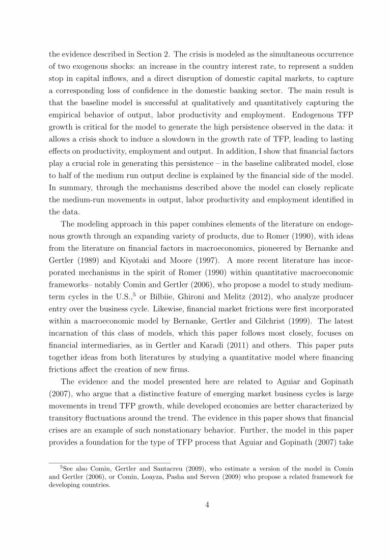
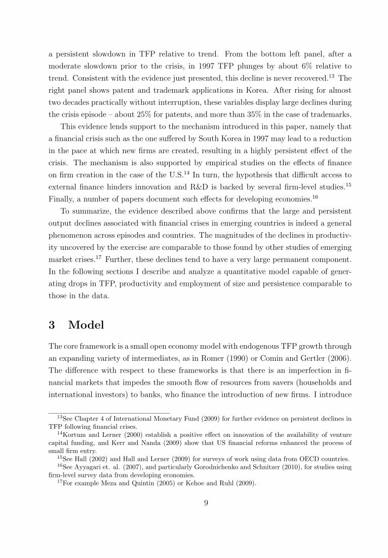
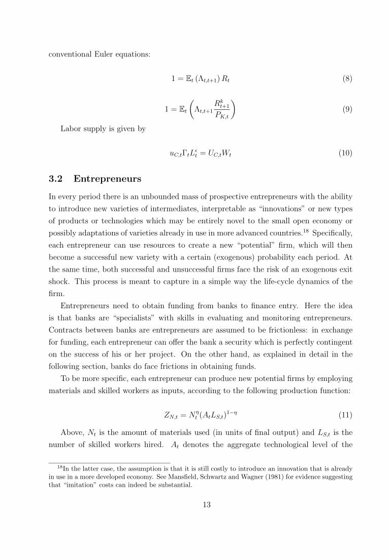
I now turn to describing the empirical exercise. Figure 1 provides some suggestive ev-
idence: it plots (log) output, labor productivity and employment for a group of Asian
countries around the financial crisis of 1997.7 The first panel suggests a very persistent
output loss following the crisis: output does not recover to the pre-crisis trend (green
dashed line), but rather remains permanently below trend in the aftermath of the crisis.
From the second and third panels, there is a considerable decline in labor productivity,
which is also very persistent, and a more modest slowdown in employment. In particular,
labor productivity falls by about 10 percent relative to the pre-crisis trend, and it never
rebounds.8
To provide more formal evidence on the behavior of output, labor productivity and
employment following financial crises, I employ an approach similar to Cerra and Saxena
(2008), who estimate a univariate autoregressive model for output growth, augmented to
6For instance, Gopinath and Neiman (2011), Benjamin and Meza (2009), Meza and Quintin (2007),Kehoe and Ruhl (2009), Pratap and Urrutia (2010) or Aoki, Benigno and Kiyotaki (2007).
7The countries included are Indonesia, Malaysia, Phillipines, Korea, Thailand and Hong Kong,labelled “SEA-6”. Area totals are computed by adding constant dollar, PPP-adjusted GDP for each ofthe countries. Labor productivity is defined as output per employed worker. See Appendix 1 for detailson the data.
8This is robust to different choices for the period used to compute the pre-crisis trend. Annualizedgrowth of labor productivity for the period 1980-1996 is 4.06%, which is close to that for the entirepre-crisis sample (1960-1996), equal to 3.69%. Annual productivity growth for the post-crisis period of1998-2007 is 3.61%, close to the figure for the pre-crisis sample.
5
include current and lagged values of dummies indicating financial crises and other shocks.
I start by decomposing (log) output as the sum of employment and labor productivity
(ni,t and zi,t respectively, in logs):
log(Yi,t) = log(Ni,t) + log(Yi,tNi,t
) ≡ ni,t + zi,t
I then estimate the following bivariate model:
xi,t = xi + Axi,t−1 +4∑j=0
BjDi,t + εi,t (1)
where xi,t =
[∆ni,t
∆zi,t
].
The specification is motivated by the assumption that both hours and labor pro-
ductivity are integrated of order one, so that first-differencing is necessary to achieve
stationarity.9 The regressors in (1) include a country fixed effect, one lag of the endoge-
nous vector, and current and lagged values of a dummy variable Di,t indicating the year
in which a systemic banking crisis starts in country i, year t. Lag selection procedures
recommend one lag for the endogenous vector. I include four lags for the crisis indicator
since coefficients on lags above 4 are insignificant, although results are robust to the
inclusion of a larger number of lags of Di,t.
The model in (1) is estimated on a sample of 17 emerging economies. Data for annual
real output and employment are obtained from the Total Economy Database. I obtain
systemic banking crisis dates from Laeven and Valencia (2012), an updated version of
the dates in Caprio and Klingebiel (2003), also used by Cerra and Saxena (2008) among
many others.10
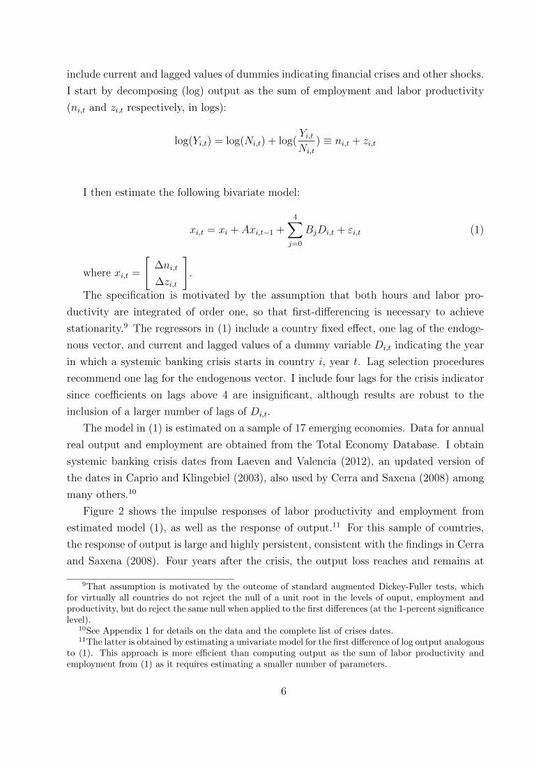
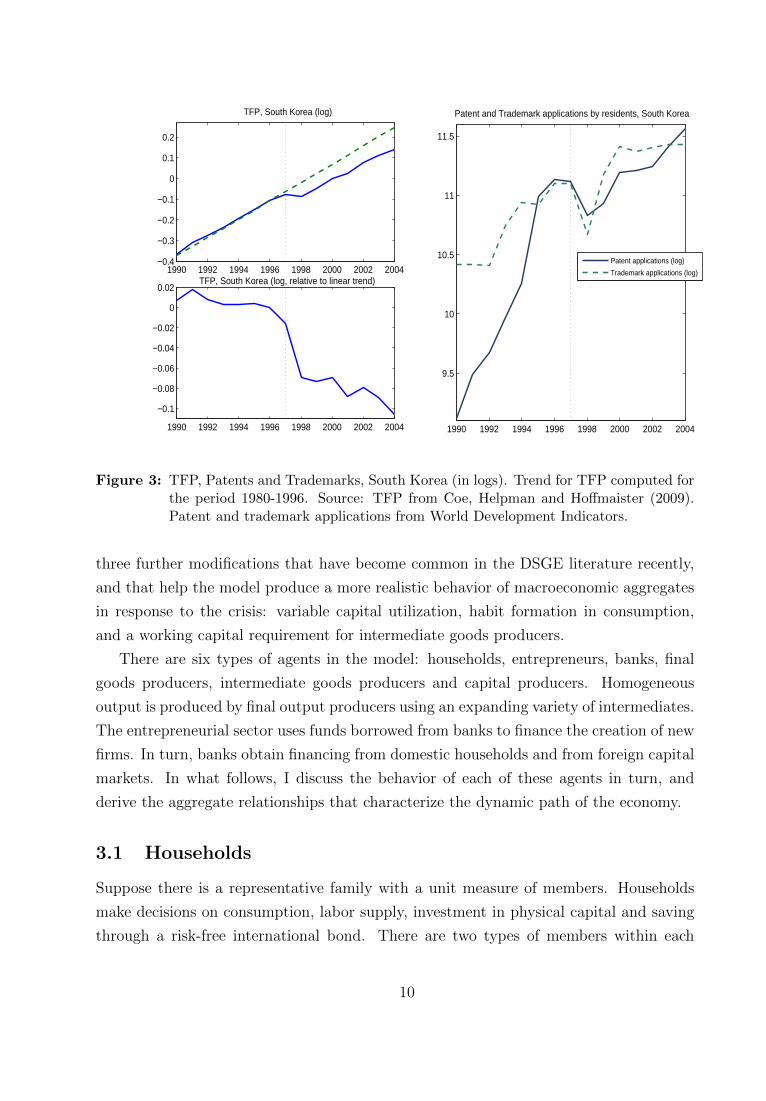
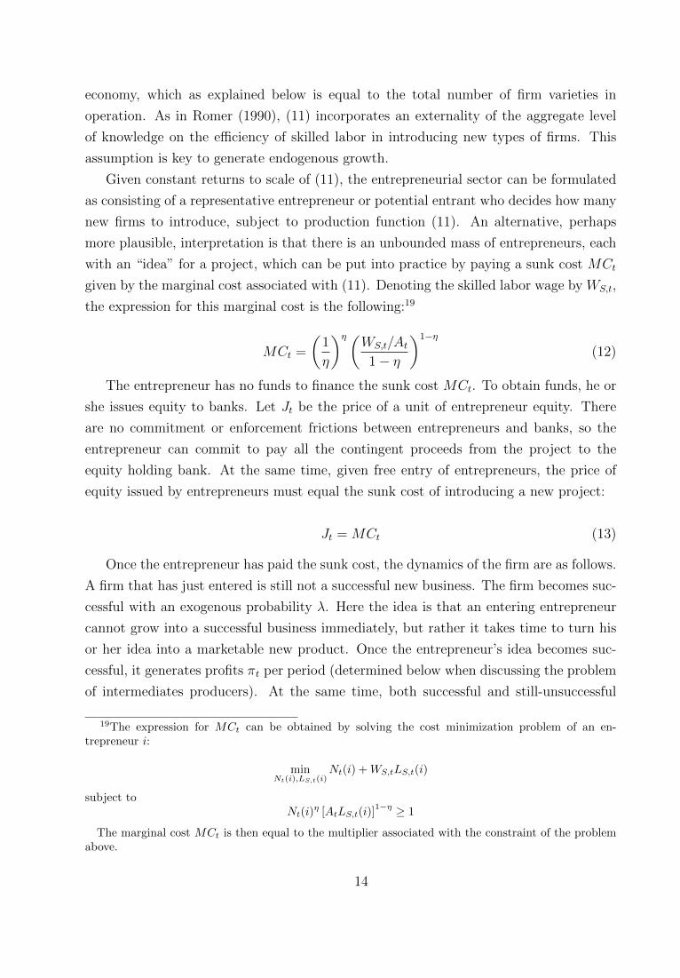
Figure 2 shows the impulse responses of labor productivity and employment from
estimated model (1), as well as the response of output.11 For this sample of countries,
the response of output is large and highly persistent, consistent with the findings in Cerra
and Saxena (2008). Four years after the crisis, the output loss reaches and remains at
9That assumption is motivated by the outcome of standard augmented Dickey-Fuller tests, whichfor virtually all countries do not reject the null of a unit root in the levels of ouput, employment andproductivity, but do reject the same null when applied to the first differences (at the 1-percent significancelevel).
10See Appendix 1 for details on the data and the complete list of crises dates.11The latter is obtained by estimating a univariate model for the first difference of log output analogous
to (1). This approach is more efficient than computing output as the sum of labor productivity andemployment from (1) as it requires estimating a smaller number of parameters.
6
1980 1985 1990 1995 2000 2005 2010
14
15
16Output for SEA−6 (log)
1980 1985 1990 1995 2000 2005 20102
2.5
3
Labor Productivity for SEA−6 (log)
1980 1985 1990 1995 2000 2005 201011.5
12
12.5Employment for SEA−6 (log)
Figure 1: Total output, employment and output per employed worker (logs) for group of 6South East Asian countries (Indonesia, Malaysia, Phillipines, Korea, Thailand andHong Kong). Pre-crisis linear trend (green dashed line) computed for the period1980-1996.
7
0 2 4 6 8 10
−0.14
−0.12
−0.1
−0.08
−0.06
−0.04
−0.02
0
Labor Productivity
Years
0 2 4 6 8 10
−0.14
−0.12
−0.1
−0.08
−0.06
−0.04
−0.02
0
Employment
Years
0 2 4 6 8 10
−0.14
−0.12
−0.1
−0.08
−0.06
−0.04
−0.02
0
Output
Years
Figure 2: Estimated impulse responses to a banking crisis. The dashed lines indicate 90% con-fidence bands computed by bootstrapping. Time measured in years. All variablesin logs.
almost 12 percent. Decomposing output into labor productivity and employment reveals
a substantial decline in productivity, which remains at about negative 6 percent after 4
years. From the panel on the right, the drop in employment is slightly more modest in
magnitude, and it is also highly persistent. The impulse responses reported in Figure 2
constitute the data moments against which I will evaluate the model presented below.12
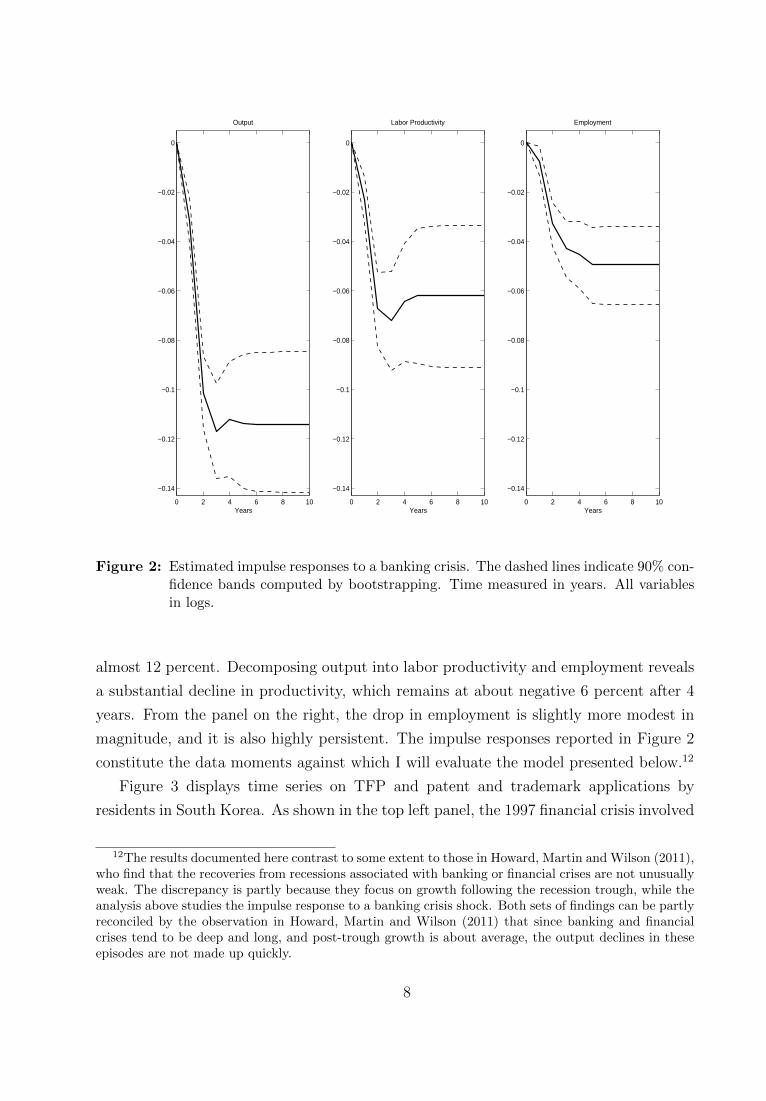
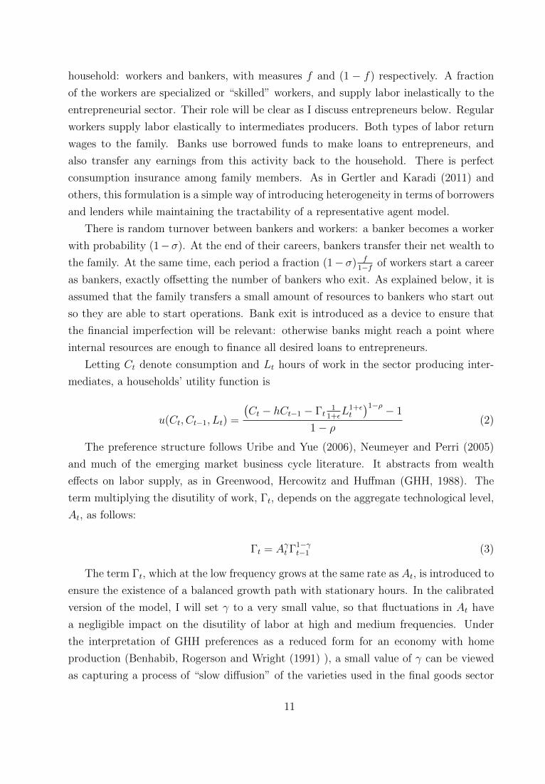
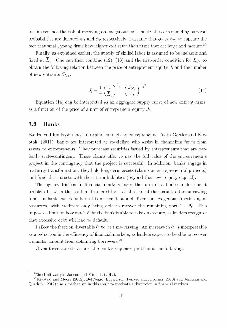
Figure 3 displays time series on TFP and patent and trademark applications by
residents in South Korea. As shown in the top left panel, the 1997 financial crisis involved
12The results documented here contrast to some extent to those in Howard, Martin and Wilson (2011),who find that the recoveries from recessions associated with banking or financial crises are not unusuallyweak. The discrepancy is partly because they focus on growth following the recession trough, while theanalysis above studies the impulse response to a banking crisis shock. Both sets of findings can be partlyreconciled by the observation in Howard, Martin and Wilson (2011) that since banking and financialcrises tend to be deep and long, and post-trough growth is about average, the output declines in theseepisodes are not made up quickly.
8
a persistent slowdown in TFP relative to trend. From the bottom left panel, after a
moderate slowdown prior to the crisis, in 1997 TFP plunges by about 6% relative to
trend. Consistent with the evidence just presented, this decline is never recovered.13 The
right panel shows patent and trademark applications in Korea. After rising for almost
two decades practically without interruption, these variables display large declines during
the crisis episode – about 25% for patents, and more than 35% in the case of trademarks.
This evidence lends support to the mechanism introduced in this paper, namely that
a financial crisis such as the one suffered by South Korea in 1997 may lead to a reduction
in the pace at which new firms are created, resulting in a highly persistent effect of the
crisis. The mechanism is also supported by empirical studies on the effects of finance
on firm creation in the case of the U.S.14 In turn, the hypothesis that difficult access to
external finance hinders innovation and R&D is backed by several firm-level studies.15
Finally, a number of papers document such effects for developing economies.16
To summarize, the evidence described above confirms that the large and persistent
output declines associated with financial crises in emerging countries is indeed a general
phenomenon across episodes and countries. The magnitudes of the declines in productiv-
ity uncovered by the exercise are comparable to those found by other studies of emerging
market crises.17 Further, these declines tend to have a very large permanent component.
In the following sections I describe and analyze a quantitative model capable of gener-
ating drops in TFP, productivity and employment of size and persistence comparable to
those in the data.
3 Model
The core framework is a small open economy model with endogenous TFP growth through
an expanding variety of intermediates, as in Romer (1990) or Comin and Gertler (2006).
The difference with respect to these frameworks is that there is an imperfection in fi-
nancial markets that impedes the smooth flow of resources from savers (households and
international investors) to banks, who finance the introduction of new firms. I introduce
13See Chapter 4 of International Monetary Fund (2009) for further evidence on persistent declines inTFP following financial crises.
14Kortum and Lerner (2000) establish a positive effect on innovation of the availability of venturecapital funding, and Kerr and Nanda (2009) show that US financial reforms enhanced the process ofsmall firm entry.
15See Hall (2002) and Hall and Lerner (2009) for surveys of work using data from OECD countries.16See Ayyagari et. al. (2007), and particularly Gorodnichenko and Schnitzer (2010), for studies using
firm-level survey data from developing economies.17For example Meza and Quintin (2005) or Kehoe and Ruhl (2009).
9
1990 1992 1994 1996 1998 2000 2002 2004−0.4
−0.3
−0.2
−0.1
0
0.1
0.2
TFP, South Korea (log)
1990 1992 1994 1996 1998 2000 2002 2004
−0.1
−0.08
−0.06
−0.04
−0.02
0
0.02TFP, South Korea (log, relative to linear trend)
1990 1992 1994 1996 1998 2000 2002 2004
9.5
10
10.5
11
11.5
Patent and Trademark applications by residents, South Korea
Patent applications (log)
Trademark applications (log)
Figure 3: TFP, Patents and Trademarks, South Korea (in logs). Trend for TFP computed forthe period 1980-1996. Source: TFP from Coe, Helpman and Hoffmaister (2009).Patent and trademark applications from World Development Indicators.
three further modifications that have become common in the DSGE literature recently,
and that help the model produce a more realistic behavior of macroeconomic aggregates
in response to the crisis: variable capital utilization, habit formation in consumption,
and a working capital requirement for intermediate goods producers.
There are six types of agents in the model: households, entrepreneurs, banks, final
goods producers, intermediate goods producers and capital producers. Homogeneous
output is produced by final output producers using an expanding variety of intermediates.
The entrepreneurial sector uses funds borrowed from banks to finance the creation of new
firms. In turn, banks obtain financing from domestic households and from foreign capital
markets. In what follows, I discuss the behavior of each of these agents in turn, and
derive the aggregate relationships that characterize the dynamic path of the economy.
3.1 Households
Suppose there is a representative family with a unit measure of members. Households
make decisions on consumption, labor supply, investment in physical capital and saving
through a risk-free international bond. There are two types of members within each
10
household: workers and bankers, with measures f and (1 − f) respectively. A fraction
of the workers are specialized or “skilled” workers, and supply labor inelastically to the
entrepreneurial sector. Their role will be clear as I discuss entrepreneurs below. Regular
workers supply labor elastically to intermediates producers. Both types of labor return
wages to the family. Banks use borrowed funds to make loans to entrepreneurs, and
also transfer any earnings from this activity back to the household. There is perfect
consumption insurance among family members. As in Gertler and Karadi (2011) and
others, this formulation is a simple way of introducing heterogeneity in terms of borrowers
and lenders while maintaining the tractability of a representative agent model.
There is random turnover between bankers and workers: a banker becomes a worker
with probability (1−σ). At the end of their careers, bankers transfer their net wealth to
the family. At the same time, each period a fraction (1− σ) f1−f of workers start a career
as bankers, exactly offsetting the number of bankers who exit. As explained below, it is
assumed that the family transfers a small amount of resources to bankers who start out
so they are able to start operations. Bank exit is introduced as a device to ensure that
the financial imperfection will be relevant: otherwise banks might reach a point where
internal resources are enough to finance all desired loans to entrepreneurs.
Letting Ct denote consumption and Lt hours of work in the sector producing inter-
mediates, a households’ utility function is
u(Ct, Ct−1, Lt) =
(Ct − hCt−1 − Γt
11+ε
L1+εt
)1−ρ − 1
1− ρ(2)
The preference structure follows Uribe and Yue (2006), Neumeyer and Perri (2005)
and much of the emerging market business cycle literature. It abstracts from wealth
effects on labor supply, as in Greenwood, Hercowitz and Huffman (GHH, 1988). The
term multiplying the disutility of work, Γt, depends on the aggregate technological level,
At, as follows:
Γt = Aγt Γ1−γt−1 (3)
The term Γt, which at the low frequency grows at the same rate as At, is introduced to
ensure the existence of a balanced growth path with stationary hours. In the calibrated
version of the model, I will set γ to a very small value, so that fluctuations in At have
a negligible impact on the disutility of labor at high and medium frequencies. Under
the interpretation of GHH preferences as a reduced form for an economy with home
production (Benhabib, Rogerson and Wright (1991) ), a small value of γ can be viewed
as capturing a process of “slow diffusion” of the varieties used in the final goods sector
11
into the home production sector.
The households’ decision problem is to choose stochastic sequences for consumption,
labor supply, purchases of the international bond and purchases of following-period phys-
ical capital to solve the following problem:
max(Ci,Li,DFi ,Ki+1)
Et∞∑i=0
βiu(Ct+i, Lt+i)
subject to
Ct + PK,tKt+1 ≤ RktKt +WtLt +
1
Rt
DFt −DF
t−1 + τ t
Above, PK,t is the price of capital and Rkt is its rental rate, Wt the wage rate and Rt
is the interest rate on the international bond. DFt denotes the family’s choice of foreign
debt and Kt+1 is the choice for physical capital holdings. Finally, τ t denotes net transfers
from firm ownership plus wages earned by skilled workers.
The international interest rate Rt depends on aggregate net foreign indebtedness Bt
and on a random shock rt as follows:
Rt = r + ert + ψ[eBt−BYt − 1
](4)
As is usual in the small open economy literature, the reason for introducing a de-
pendence of the cost of borrowing on net foreign indebtedness is to ensure stationary
dynamics. I choose a very small value for ψ so that this feature does not affect the
dyamics of the model. A raise in rt, interpretable as a country interest rate shock, is
a simple way to model the sudden capital outflows that have accompanied many of the
emerging market financial crises analyzed in the previous section. The expression for
marginal utility of consumption, UC,t is the following:
UC,t = uC,t − βγEt (uC,t+1) (5)
uC,t =
(Ct − hCt−1 − Γt
1
1 + εL1+εt
)−ρ(6)
Define the households’ stochastic discount factor between periods t and t + i, Λt,t+i
as
Λt,t+i ≡βUC,t+iUC,t
(7)
Then the household’s decision on bond and capital holdings are characterized by two
12
conventional Euler equations:
1 = Et (Λt,t+1)Rt (8)
1 = Et(
Λt,t+1
Rkt+1
PK,t
)(9)
Labor supply is given by
uC,tΓtLεt = UC,tWt (10)
3.2 Entrepreneurs
In every period there is an unbounded mass of prospective entrepreneurs with the ability
to introduce new varieties of intermediates, interpretable as “innovations” or new types
of products or technologies which may be entirely novel to the small open economy or
possibly adaptations of varieties already in use in more advanced countries.18 Specifically,
each entrepreneur can use resources to create a new “potential” firm, which will then
become a successful new variety with a certain (exogenous) probability each period. At
the same time, both successful and unsuccessful firms face the risk of an exogenous exit
shock. This process is meant to capture in a simple way the life-cycle dynamics of the
firm.
Entrepreneurs need to obtain funding from banks to finance entry. Here the idea
is that banks are “specialists” with skills in evaluating and monitoring entrepreneurs.
Contracts between banks are entrepreneurs are assumed to be frictionless: in exchange
for funding, each entrepreneur can offer the bank a security which is perfectly contingent
on the success of his or her project. On the other hand, as explained in detail in the
following section, banks do face frictions in obtaining funds.
To be more specific, each entrepreneur can produce new potential firms by employing
materials and skilled workers as inputs, according to the following production function:
ZN,t = Nηt (AtLS,t)
1−η (11)
Above, Nt is the amount of materials used (in units of final output) and LS,t is the
number of skilled workers hired. At denotes the aggregate technological level of the
18In the latter case, the assumption is that it is still costly to introduce an innovation that is alreadyin use in a more developed economy. See Mansfield, Schwartz and Wagner (1981) for evidence suggestingthat “imitation” costs can indeed be substantial.
13
economy, which as explained below is equal to the total number of firm varieties in
operation. As in Romer (1990), (11) incorporates an externality of the aggregate level
of knowledge on the efficiency of skilled labor in introducing new types of firms. This
assumption is key to generate endogenous growth.
Given constant returns to scale of (11), the entrepreneurial sector can be formulated
as consisting of a representative entrepreneur or potential entrant who decides how many
new firms to introduce, subject to production function (11). An alternative, perhaps
more plausible, interpretation is that there is an unbounded mass of entrepreneurs, each
with an “idea” for a project, which can be put into practice by paying a sunk cost MCt
given by the marginal cost associated with (11). Denoting the skilled labor wage by WS,t,
the expression for this marginal cost is the following:19
MCt =
(1
η
)η (WS,t/At1− η
)1−η
(12)
The entrepreneur has no funds to finance the sunk cost MCt. To obtain funds, he or
she issues equity to banks. Let Jt be the price of a unit of entrepreneur equity. There
are no commitment or enforcement frictions between entrepreneurs and banks, so the
entrepreneur can commit to pay all the contingent proceeds from the project to the
equity holding bank. At the same time, given free entry of entrepreneurs, the price of
equity issued by entrepreneurs must equal the sunk cost of introducing a new project:
Jt = MCt (13)
Once the entrepreneur has paid the sunk cost, the dynamics of the firm are as follows.
A firm that has just entered is still not a successful new business. The firm becomes suc-
cessful with an exogenous probability λ. Here the idea is that an entering entrepreneur
cannot grow into a successful business immediately, but rather it takes time to turn his
or her idea into a marketable new product. Once the entrepreneur’s idea becomes suc-
cessful, it generates profits πt per period (determined below when discussing the problem
of intermediates producers). At the same time, both successful and still-unsuccessful
19The expression for MCt can be obtained by solving the cost minimization problem of an en-trepreneur i:
minNt(i),LS,t(i)
Nt(i) +WS,tLS,t(i)
subject toNt(i)
η [AtLS,t(i)]1−η ≥ 1
The marginal cost MCt is then equal to the multiplier associated with the constraint of the problemabove.
14
businesses face the risk of receiving an exogenous exit shock: the corresponding survival
probabilities are denoted φA and φZ respectively. I assume that φA > φZ , to capture the
fact that small, young firms have higher exit rates than firms that are large and mature.20
Finally, as explained earlier, the supply of skilled labor is assumed to be inelastic and
fixed at LS. One can then combine (12), (13) and the first-order condition for LS,t to
obtain the following relation between the price of entrepreneur equity Jt and the number
of new entrants ZN,t:
Jt =1
η
(1
LS
) 1−ηη(ZN,tAt
) 1−ηη
(14)
Equation (14) can be interpreted as an aggregate supply curve of new entrant firms,
as a function of the price of a unit of entrepreneur equity Jt.
3.3 Banks
Banks lend funds obtained in capital markets to entrepreneurs. As in Gertler and Kiy-
otaki (2011), banks are interpreted as specialists who assist in channeling funds from
savers to entrepreneurs. They purchase securities issued by entrepreneurs that are per-
fectly state-contingent. These claims offer to pay the full value of the entrepreneur’s
project in the contingency that the project is successful. In addition, banks engage in
maturity transformation: they hold long-term assets (claims on entrepreneurial projects)
and fund these assets with short-term liabilities (beyond their own equity capital).
The agency friction in financial markets takes the form of a limited enforcement
problem between the bank and its creditors: at the end of the period, after borrowing
funds, a bank can default on his or her debt and divert an exogenous fraction θt of
resources, with creditors only being able to recover the remaining part 1 − θt. This
imposes a limit on how much debt the bank is able to take on ex-ante, as lenders recognize
that excessive debt will lead to default.
I allow the fraction divertable θt to be time-varying. An increase in θt is interpretable
as a reduction in the efficiency of financial markets, as lenders expect to be able to recover
a smaller amount from defaulting borrowers.21
Given these considerations, the bank’s sequence problem is the following:
20See Haltiwanger, Jarmin and Miranda (2012).21Kiyotaki and Moore (2012), Del Negro, Eggertsson, Ferrero and Kiyotaki (2010) and Jermann and
Quadrini (2012) use a mechanism in this spirit to motivate a disruption in financial markets.
15
maxst+i−1,dt+i−1∞i=1
[Et
∞∑i=1
σi−1(1− σ)Λt,t+i φZ [λvt+i + (1− λ)Jt+i] st+i−1 −Rt+i−1dt+i−1
](15)
subject to
Jtst +Rt−1dt−1 ≤ φZ [λvt + (1− λ)Jt] st−1 + dt (16)
Et∞∑i=1
σi−1(1− σ)Λt,t+i φZ [λvt+i + (1− λ)Jt+i] st+i−1 −Rt+i−1dt+i−1 ≥ θtJtst (17)
Examining first the budget constraint, equation (16), the bank’s use of funds (left
hand side) includes the purchase of an amount st of claims on entrepreneurs, which costs
Jtst, as well as debt repayments, Rt−1dt−1. The sources of funds are the revenues obtained
from previous loans (the first term on the right hand side) as well as new debt issued,
dt. Projects financed the previous period, st−1, have a survival probability φZ . If the
project survives, it is successful with probability λ, in which case the bank receives its
full value, denoted vt. If the project is unsuccessful this period, then given the simple
Poisson process for the evolution of projects it is exactly equivalent to a security issued
by a new entrant entrepreneur, so that its value is Jt.
A successful project generates a stream of profits πt+i∞i=0 obtained from manufac-
turing and selling the new variety of intermediate. Therefore, the value of a successful
project is given by the expected discounted value of the profit stream, accounting for the
survival rate φA of successful firms:22
vt = Et
[∞∑i=0
φiAΛt,t+iπt+i
](18)
As indicated by (15), if a bank alive at t exits in period t + i (which happens with
probability σi−1(1−σ)) it the accumulated wealth back to the household. The resources
accumulated until period t + i are given by the term in curly brackets in (15). The
bank thus values payoffs in the period and state at which it exits with the household’s
22Here the underlying assumption is that the entrepreneur, when successful, sells the idea to a mo-nopolist producer of intermediates, who then obtains the stream of profits πt+i∞i=0 from manufacturingand selling the new variety and therefore is willing to pay vt for the project.
16

stochastic discount factor, Λt,t+i.
Equation (17) is the bank’s incentive constraint. At the end of period t, after having
borrowed in capital markets, the bank may choose to default on its creditors and divert
fraction θt of available funds, which it then transfers back to its household. Creditors
can then force the bank into bankruptcy and recover the remaining fraction 1 − θt of
resources, but it is too costly for them to recover the fraction θt of funds that the bank
diverted. Accordingly, for creditors to be willing to supply funds to the bank, equation
(17) must hold: the bank’s value if he honors the contract with his creditors must be
greater than the value of diverting resources in the amount θtJtst and being shut down.
To simplify the bank’s problem, define first the rate of return to one dollar invested
in entrepreneurial projects, RZ,t:
RZ,t ≡ φZλvt + (1− λ)Jt
Jt−1
RZ,t depends only on the aggregate state, through prices vt and Jt. Times of low
realizations of the value of a new intermediate, vt and of the value of entrepreneur equity,
Jt, will be times of low returns RZ,t. Noting that bank’s individual state variables at
the beginning of period t are st−1 and dt−1, the entrepreneur’s problem can be expressed
recursively as follows:
Vt(st−1, dt−1) = maxst,dt
(1− σ)Et [Λt,t+1 (RZ,t+1Jtst −Rtdt)] + σEt [Λt,t+1Vt+1(st, dt)] (19)
subject to
Jtst +Rt−1dt−1 ≤ RZ,tJt−1st−1 + dt (20)
(1− σ)Et [Λt,t+1 (RZ,t+1Jtst −Rtdt)] + σEt [Λt,t+1Vt+1(st, dt)] ≥ θtJtst (21)
Above, the time index on the value function reflects aggregate uncertainty. The
problem can be simplified further by realizing that the key individual state variable is
the bank’s net worth wt, defined as the difference between the value of assets and debt:
wt ≡ Jtst − dt (22)
From the budget constraint (20) at equality, the evolution of net worth is
17

wt = (RZ,t −Rt−1)Jt−1st−1 +Rt−1wt−1 (23)
Net worth at t is given by the gross return to the bank’s investments financed during
t − 1, net of repayments to creditors. Equation (23) shows that net worth at t depends
on the individual state at t− 1 (st−1, wt−1) together with the realization of the aggregate
state at t, through the rate of return RZ,t. This suggests making the following guess for
the bank’s value function:
Vt(st−1, dt−1) = Ωtwt (24)
Above, the undetermined coefficient Ωt is conjectured to depend only on the aggregate
state, and dependence of wt on (st−1, dt−1) through (22) and (23) is understood. Define
also the following variables:
Ωt+1 ≡ 1− σ + σΩt+1 (25)
µt ≡ Et [Λt,t+1Ωt+1 (RZ,t+1 −Rt)] (26)
νt ≡ Et (Λt,t+1Ωt+1)Rt (27)
Variable Ωt+1 is interpretable as the prospective value of a unit of net worth, before
the bank finds out whether he will have to exit at the end of the period. From equation
(26), µt is interpretable to the return for the bank of investing in excess of the cost of
funds. Finally, νt represents the value of an extra unit of net worth today.
Given the definitions above, the problem of the bank reduces to the following:
Ωtwt = maxst
µtJtst + νtwt (28)
subject to
µtJtst + νtwt ≥ θtJtst (29)
Here µt reflects the value to the bank of funding an additional project (increasing st)
while holding net worth constant. On the other hand, νt is the value of an additional
unit of net worth, holding constant st. With frictionless financial markets banks would
be unconstrained, with the implication that µt = 0. The agency problem introduces a
friction that makes banks potentially constrained, and that may therefore place limits
on arbitrage.
18
Equation (29) is the incentive constraint. Note that as long as µt ≥ 0, it is profitable
for the bank to borrow and fund an additional project. Thus, in this instance, and given
wt > 0, the constraint binds:
Jtst =νt
θt − µtwt (30)
Equation (30) shows that the amount the bank can spend on funding projects, Jtst,
is constrained by his net worth wt, through a limit on the amount the bank is allowed to
borrow in capital markets.23
Define the banks maximum leverage ratio φt as
φt ≡νt
θt − µt(31)
so that when the credit constraint binds,
Jtst = φtwt (32)
Then with a binding constraint, solving the undetermined coefficient from (28)-(29)
we have that
Ωt = µtφt + νt (33)
The value of a unit of net worth today (Ωt) derives from its value holding assets
constant (νt) plus the capacity that it generates to fund additional projects (φt) multiplied
by the value to the bank of those additional projects (µt).
3.3.1 Aggregation
Aggregation accross banks is simple given the linearity of (32). The aggregate amount of
projects funded, St, is constrained by aggregate net worth of the financial intermediation
sector:
JtSt = φtWt (34)
At the same time, aggregate net worth at t is given by the sum of net worth of
surviving banks, which evolves individually according to (23), and the transfer that
23Note that for the incentive constraint to bind we must also have µt < θt: otherwise, the value of anextra project is greater than the gain from diverting the additional funds, so there is never an incentiveto default. In the equilibrium constructed below, for reasonable parameterizations the constraint alwaysbinds along the balanced growth path.
19
newborn ones obtain from their family. For simplicity I assume that the transfer is a
small fraction ξ of the total value of the projects funded the previous period. Accordingly,
the law of motion of aggregate net worth is given by
Wt = σ [(RZ,t −Rt−1) Jt−1St−1 +Rt−1Wt−1] + (1− σ)ξJt−1St−1 (35)
Note that the source of fluctuations in aggregate net worth of the financial intermedia-
tion sector are movements in return RZ,t, which as discussed earlier arise from movements
in the prices vt and Jt.
In what follows I describe the evolution of the aggregate stock of projects for new
varieties. At the beginning of period t, a total number of potential firms Zt exist in the
economy. Each point in [0, Zt] represents a project for a different intermediate. The points
between 0 and At correspond to already successful new intermediates, with At < Zt. In
period t, the entrepreneurial sector introduces a measure ZN,t of new potential firms.
At the same time, a fraction 1 − φZ of unsuccessful firms exit each period. Thus, the
aggregate number of potential firms Zt evolves as follows:
Zt+1 = φZ (Zt + ZN,t) (36)
In period t the points between At and Zt + ZN,t correspond to projects “in process”,
i.e. projects that the entrepreneurial sector is currently attempting to turn into successful
firms. Fraction λ of these projects will become successful during period t. Also, only
fraction φA of firms operating in period t survive into t+ 1. Therefore, the total number
of varieties of intermediates, At, evolves as follows:
At+1 = λ [φZ (Zt + ZN,t)− At] + φAAt (37)
where the term in brackets is the measure of potential firms that have not yet been
successful, accounting for the fact that only fraction φZ of potential firms survive each
period.
Recall that St refers to the aggregate number of projects financed by banks. In
equilibrium, we must have
St = φZ (Zt + ZN,t)− At (38)
That is, the total number of projects financed by the financial intermediation sector
must be equal to the total number of projects that entrepreneurs are currently holding
and trying to develop.
20
These considerations clarify how financial factors may affect the evolution of TFP.
When net worth is low, through equation (34) the aggregate number of projects that
the intermediation sector can finance, St, is reduced. This makes demand for new en-
trants ZN,t lower, as equation (38) suggests. With a smaller number of products being
attempted, the growth rate of TFP will decline, as equation (37) indicates.
3.3.2 The Frictionless Benchmark
As emphasized earlier, with frictionless markets there is perfect arbitrage, so that excess
returns µt must be equal to zero. It follows from (25)-(27) and (33) that Et(Λt,t+1RZ,t+1) =
Et(Λt,t+1)Rt = 1, or
Jt = Et Λt,t+1φZ [λvt+1 + (1− λ)Jt+1] (39)
The value of entrepreneur equity, Jt, is given by the option value of obtaining a suc-
cessful new intermediate the following period, valued vt+1 – this happens with probability
λ. With financial frictions and constrained banks, we will have
Jt < Et Λt,t+1φZ [λvt+1 + (1− λ)Jt+1] (40)
The gap between the left and right hand side of (40) widens whenever banks’ fi-
nancial constraints are tighter, which happens in times in which the net worth of the
intermediation sector is low. This implies that the rate of new firm creation falls below
its frictionless level. The imperfection in financial markets also implies that the growth
rate of TFP, and therefore of output, along the balanced growth path is below its value
in a model without financial frictions.24
3.4 Final Output and Intermediates Producers
The final good is produced in a competitive sector which aggregates a continuum of
measure At of intermediates:
Yt =
[∫ At
0
Yt(s)ϑ−1ϑ ds
] ϑϑ−1
(41)
Given the aggregator above, demand for each intermediate s by the final good sector
is
24See Levine (1997, 2005) for surveys of evidence suggesting that financial development has a positiveimpact on long-run TFP and output growth.
21
Yt(s) =
[Pt(s)
Pt
]−ϑYt (42)
where the price level Pt is defined as
Pt =
[∫ At
0
Pt(s)1−ϑds
] 11−ϑ
(43)
Equation (42) gives the demand facing each intermediate good producer s. Inter-
mediates are produced using a standard Cobb-Douglas technology with capital services
ut(s)Kt(s) and labor Lt(s) as inputs:
Yt(s) = [ut(s)Kt(s)]α Lt(s)
1−α (44)
Intermediate goods firms face a working capital requirement which forces them to
hold an amount of non-interest-bearing assets that is no smaller than a multiple θW of
the quarterly wage bill:
κt(s) ≥ θWWtLt(s) θW ≥ 0
where κt(s) denotes the amount of working capital held by firm s in period t. As
shown in Uribe and Yue (2006) and Mendoza and Yue (2012), this formulation implies
that the effective cost of labor becomes[1 + θW
(Rt−1Rt
)]Wt, and therefore an increase
in the interest rate reduces the demand of labor by intermediates firms.
The objective of intermediates producers is to maximize profits, including the value
of the remaining part of capital they rent from households. Firms face a replacement
price of depreciated capital equal to unity.25 Thus, their objective is to solve
πt = maxPt(s), Yt(s),
ut(s),Kt(s),
Lt(s)
Pt(s)Yt(s)+PK,tKt(s)−δ(ut(s))Kt(s)−[1 + θW
(Rt − 1
Rt
)]WtLt(s)−Rk
tKt(s)
Subject to (42) and (44). Solving the firm’s problem yields the following equations:[1 + θW
(Rt − 1
Rt
)]Wt = (1− α)
YtLt
(45)
25As made clear below, adjustment costs are on net rather than gross investment, so that replacingworn-out capital does not involve adjustment costs. This formulation makes the capital utilizationdecision independent of the price of capital.
22
Rkt = α
YtKt
+ PK,t − δ(ut) (46)
αYtut
= δ′(ut)Kt (47)
Each intermediates producer sets its price to a constant markup over marginal cost
– the ratio of price to marginal cost equals ϑϑ−1
. Per period profits of intermediates
producers, πt, can then be shown to be equal to
πt =1
ϑ
YtAt
(48)
Finally, one can combine (41) with the first-order conditions for intermediates pro-
ducers and with equilibrium in factor markets to obtain an expression for final output:
Yt = A1
ϑ−1
t (utKt)αL1−α
t (49)
3.5 Capital Producers
At the end of period t, capital producing firms repair depreciated capital and produce
new capital. For simplicity I assume that no financial frictions apply to the production
and purchase of capital goods, in order to focus on the role of frictions on the creation
of new firms. However, it would be straightforward to extend the model to allow for
frictions in investment of existing firms as well, along the lines of Gertler and Karadi
(2011) and others.26
As in and Gertler et. al. (2007), repair of old capital is not subject to adjustment
costs, but there are stock adjustment costs associated with the production of new capital.
Let Int be net investment, the amount of investment used for construction of new capital
goods:
Int = It − δ(ut)Kt (50)
To produce new capital, capital producers combine final output with existing capital
via the constant returns to scale technology Φ(Int /Kt)Kt, where Φ(·) is increasing and
26To elaborate on this, one could follow Gertler and Karadi (2011) and assume that firms need toobtain loans from banks to finance their purchases of physical capital. In this generalized model, bankswould then make two types of loans: loans to existing firms to invest, and loans to entrepreneurs to createnew firms. One could postulate different intensities of the financial friction for each type of activity,which could be captured by assuming that the fractions divertable are different for each of the two typesof banks’ assets.
23
concave and satisfies Φ(In/K) = 0 and Φ′(In/K) = 1, where In/K is the net investment
to capital ratio along the balanced growth path.
The economy-wide capital stock evolves according to27
Kt+1 = Kt + Φ
(IntKt
)Kt (51)
As in Gertler et. al. (2007), I assume that capital producing firms make produc-
tion plans one period in advance, with the objective of capturing the delayed response
of investment observed in the data. Accordingly, the optimality condition for capital
producers is
Et−1(PK,t) = Et−1
[Φ′(IntKt
)]−1
(52)
3.6 Market Clearing
The economy uses output and international borrowing to finance consumption, invest-
ment in physical capital, and investment in new technology. The resulting market clearing
condition is
1
Rt
Bt −Bt−1 + Yt = Ct + It +Nt (53)
Bt is economywide foreign indebtedness, equal to the sum of aggregate family and
entrepreneurial debt (Bt = DFt +Dt). Equation (53) can be derived by combining family
and entrepreneur budget constraints with equilibrium conditions.
This completes the description of the model.
4 Model Analysis
This section presents numerical results from a dynamic simulation of the model, meant
to capture in a rough way the type of crises analyzed empirically in Section 2. The
goal is to illustrate how the novel mechanism introduced in the paper, namely financially
constrained firm creation, is crucial for the model to be able to produce persistent declines
in output, productivity and employment that are quantitatively close to those identified
in the data.28
27Given the assumptions on Φ(·), to a first order the evolution of capital along the balanced growthpath is the usual Kt+1 = [1− δ(ut)]Kt + It.
28Appendix C contains some additional model results regarding the effects of non-financial shocks.
24
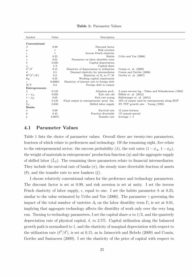
Table 1: Parameter Values
Symbol Value Description
Conventionalβ 0.99 Discount factorρ 1 Risk aversionε 1 Inverse Frisch elasticityh 0.25 Habits Uribe and Yue (2006)γ 0.01 Parameter on labor disutility termδ 0.025 Capital depreciationα 1/3 Capital shareδ′′/δ′ 0.15 Elasticity of depreciation to utilization Comin et. al. (2009)ϑ 2.5 Demand elasticity for intermediates Comin and Gertler (2006)Φ′′(In/K) 0.2 Elasticity of Pk to In/K Gertler et. al. (2007)θW 0.35 Working capital requirementι 0.00001 Elasticity of interest rate to foreign debtB/Y 0.2 Foreign debt to outputEntrepreneursλ 0.125 Adoption prob. 2 years success lag – Pakes and Schankerman (1984)1− φA 0.025 Exit rate old Bilbiie et. al. (2012)1− φZ 0.05 Exit rate young Haltiwanger et. al. (2012)η 0.125 Final output in entrepreneurs’ prod. fun. 10% of output used by entrepreneurs along BGP
LS 0.033 Skilled labor supply 2% TFP growth rate – Young (1995)Banksσ 0.98 Survival rate 12 years horizonθ 0.45 Fraction divertable 1% annual spreadξ 0.0075 Transfer rate leverage = 4
4.1 Parameter Values
Table 1 lists the choice of parameter values. Overall there are twenty-two parameters,
fourteen of which relate to preferences and technology. Of the remaining eight, five relate
to the entrepreneurial sector: the success probability (λ), the exit rates (1−φA, 1−φZ),
the weight of materials in entrepreneurs’ production function (η) and the aggregate supply
of skilled labor (LS). The remaining three parameters relate to financial intermediaries.
They include the survival rate of banks (σ), the steady state divertable fraction of assets
(θ), and the transfer rate to new bankers (ξ).
I choose relatively conventional values for the preference and technology parameters.
The discount factor is set at 0.99, and risk aversion is set at unity. I set the inverse
Frisch elasticity of labor supply, ε, equal to one. I set the habits parameter h at 0.25,
similar to the value estimated by Uribe and Yue (2006). The parameter γ governing the
impact of the total number of varieties At on the labor disutility term Γt is set at 0.01,
implying that aggregate technology affects the disutility of work only over the very long
run. Turning to technology parameters, I set the capital share α to 1/3, and the quarterly
depreciation rate of physical capital, δ, to 2.5%. Capital utilization along the balanced
growth path is normalized to 1, and the elasticity of marginal depreciation with respect to
the utilization rate (δ′′/δ′), is set at 0.15, as in Jaimovich and Rebelo (2009) and Comin,
Gertler and Santacreu (2009). I set the elasticity of the price of capital with respect to
25
the investment-capital ratio at 0.2, as in Gertler et. al. (2007) and Bernanke et. al.
(1999). I choose the parameter on the intermediate goods aggregator, ϑ, so that output
is proportional to TFP along the balanced growth path, which by examining equation
(49) amounts to imposing (1− α)(ϑ− 1) = 1. This restriction makes profits per period,
πt, a stationary variable, and simplifies somewhat the characterization of the balanced
growth path. Given α = 1/3, the resulting value for the markup is ϑ/(ϑ − 1) = 1.66,
close to the value of 1.6 chosen by Comin and Gertler (2006).
Regarding the working capital constraint, I set θW = 0.35, implying that firms need
to pay less than a month’s worth of the wage bill in advance.29 The debt to GDP ratio
along the balanced growth path is set at 0.2, and the elasticity of the interest rate with
respect to the debt-output ratio equals 0.00001 – the latter ensures that the dynamics of
the model are virtually unaffected by the debt-elastic interest rate at high and medium
frequencies, while still making the foreign asset position revert to trend over the long
run.
Turning to the parameters relating to the entrepreneurial sector, I set the probability
of successfully obtaining a new variety, λ, to 0.125, implying an average success lag ( 1λ) of
8 quarters or 2 years. This is based on evidence on mean R&D gestation lags reported by
Pakes and Schankerman (1984), defined as the average time between the initial outlay of
resources and the beginning of the associated revenue stream. The exit rate for mature
firms (1 − φA) is set to 10 percent annually, following Bilbiie et. al. (2012), and the
corresponding number for young firms (1 − φZ) is set to twice that number, consistent
with the evidence in Haltiwanger et. al. (2012) of substantially higher firm exit by
younger firms. The weight of final output in entrepreneurs’ production function, η, is set
to 0.125, implying that along the balanced growth path 10 percent of output is used by
the entrepreneurial sector. This number represents a rough estimate of expenditures on
firm creation as a fraction of GDP.30 Finally, the inelastic supply of skilled labor, LS, is
set to deliver a growth rate of TFP along the balanced growth path of 2 percent, similar
to the numbers reported by Young (1995).
The choice of the financial sector parameters is meant to be suggestive. Similar to
Gertler and Kiyotaki (2010), I set the entrepreneur survival rate σ = 0.98, implying an
expected horizon of bankers of about twelve years. To calibrate the fraction of resources
29While higher values of this parameter are frequently used in the literature, Mendoza and Yue (2012)argue that it is desirable to set this parameter at a relatively low value, since empirical estimates suggestthat working capital is a small fraction of GDP. A working capital requirement of 0.35, together with awage bill of two thirds of GDP, implies a ratio of working capital to GDP of around 23%.
30MacGrattan and Prescott (2010), for example, estimate investment in technology capital at about6 percent of GNP in the US. This is likely a lower bound on total entry costs, as not all firm creation iscaptured by R&D data.
26
that bankers can divert in steady state, θ, and the transfer to newborn bankers, ξ, I
target two features of the balanced growth path of the model economy: a bank leverage
ratio (assets to net worth) of four, and an excess return E(RZ)−R equal to one hundred
basis points annually. The target for the leverage ratio reflects a relatively conservative
attempt to capture an average leverage ratio of the financial intermediation sector. For
example, most housing finance is typically intermediated by financial institutions with
leverage ratios of at least 10 on average in the case of commercial banks, and substantially
higher for investment banks.31 On the other hand, leverage ratios are clearly smaller in
other sectors of the economy. The target for the spread along the balanced growth path
is based on evidence on BBB industrial corporate spreads in the US and Europe prior to
the crisis. These targets imply setting the divertible fraction θ to 0.45, and the transfer
rate ξ to 0.0075.
4.2 Crisis Experiment
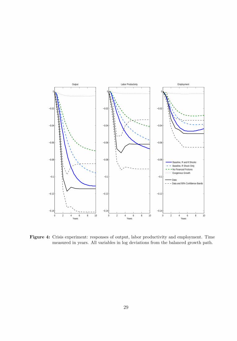
I now turn to the crisis experiment. The initiating disturbance is the combined impact
of two shocks: an increase in the country interest rate Rt, and an increase in the variable
governing the agency friction, θt.
I consider a 500 basis point increase in the interest rate that persists as a first-order
autoregressive process with a 0.88 coefficient. These magnitudes are close to the evidence
for the crisis in South Korea in 1997, as shown by Gertler et. al. (2007).32 At the same
time, θt rises by fifty percent, and the increase persists as a first order autoregressive
process with coefficient 0.95 (the time paths for Rt and θt are shown in Figure 5). The
idea is to capture a situation in which not only there is a capital outflow, as captured by
an increase in Rt, but also a disruption in domestic financial markets, corresponding in
the model to the increase in θt. It is best to think of the shock as a rare event.
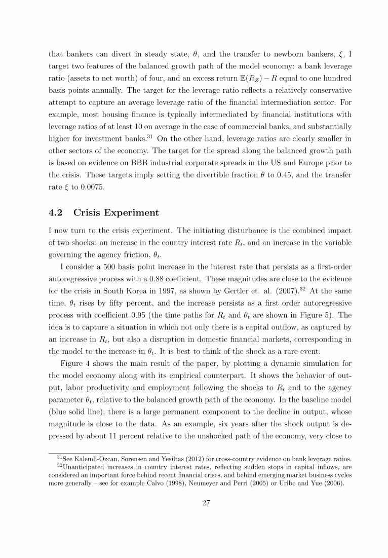
Figure 4 shows the main result of the paper, by plotting a dynamic simulation for
the model economy along with its empirical counterpart. It shows the behavior of out-
put, labor productivity and employment following the shocks to Rt and to the agency
parameter θt, relative to the balanced growth path of the economy. In the baseline model
(blue solid line), there is a large permanent component to the decline in output, whose
magnitude is close to the data. As an example, six years after the shock output is de-
pressed by about 11 percent relative to the unshocked path of the economy, very close to
31See Kalemli-Ozcan, Sorensen and Yesiltas (2012) for cross-country evidence on bank leverage ratios.32Unanticipated increases in country interest rates, reflecting sudden stops in capital inflows, are
considered an important force behind recent financial crises, and behind emerging market business cyclesmore generally – see for example Calvo (1998), Neumeyer and Perri (2005) or Uribe and Yue (2006).
27

the empirical value. This is the case even though the exogenous driving forces, Rt and
θt, have almost completely returned to their steady state values. As made clear in the
following section, behind this result is the behavior of firm creation following the crisis,
which implies that the financial crisis shock has a permanent effect on aggregate TFP.
This is the main driving force behind the behavior of labor productivity displayed in the
figure. At the same time, as shown in the last panel of Figure 4, the permanent decline
in productivity leads to a decline in labor demand by producers of intermediates. As
a result, employment also falls persistently relative to the balanced growth path of the
economy. Thus, the model is also able to account for the evidence provided in Section 2
that employment remains persistently depressed following financial crises. Overall, the
bottomline from Figure 4 is that the mechanisms introduced in the model have potential
for quantitatively accounting for the medium-run behavior of output, labor productivity
and employment following financial crises.33
The financial intermediation sector plays an important role in accounting for the
model’s behavior. Without financial market frictions (green dashed line), the responses
of all three variables differ significantly from their empirical counterparts: for example,
the decline in output six years after the shock hits is approximately 6 percent in the
case without financial frictions, compared to the 11 percent in the baseline case and
in the data. The difference is driven to a large extent by the endogenous amplification
implied the interaction between the financial intermediation sector and the process of firm
creation (described in detail in the following section). This can be seen by comparing
the case without financial frictions and the case with financial frictions but without the
shock to θt (light blue dash-dotted line). The increase in θt then contributes an extra
decline in all three variables – in the case of output its contribution is about 2 percentage
points in the medium run.
Finally, Figure 4 also reports the response in a model in which the endogenous growth
channel is inactive (grey dotted line) – what is then left is a relatively standard RBC
model of a small open economy, subjected to an interest rate shock. As made clear by
the figure, the behavior of the model in this case is very far from the data, due to the
absence of endogenous movements in TFP.
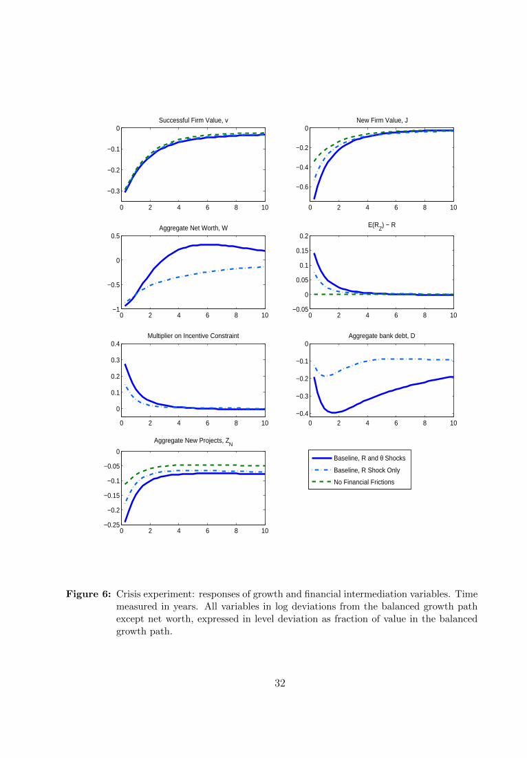
How does the model’s transmission mechanism operate? Figure 6 documents the
behavior of the financial and entrepreneurial side of the model following the crisis shock.
The disturbance induces a large decline in the value of a new variety, vt, and in the
33As Figure 4 shows, the model understates the short-run declines following the crisis. These arelikely related to phenomena like nominal price or wage rigidities which for simplicity have been ignoredin the model, focusing instead on the novel aspects regarding persistence. It would be straightforwardto extend the model along these dimensions.
28
0 2 4 6 8 10
−0.14
−0.12
−0.1
−0.08
−0.06
−0.04
−0.02
0
Output
Years
0 2 4 6 8 10
−0.14
−0.12
−0.1
−0.08
−0.06
−0.04
−0.02
0
Labor Productivity
Years0 2 4 6 8 10
−0.14
−0.12
−0.1
−0.08
−0.06
−0.04
−0.02
0
Employment
Years
Baseline, R and θ ShocksBaseline, R Shock OnlyNo Financial FrictionsExogenous Growth
DataData and 90% Confidence Bands
Figure 4: Crisis experiment: responses of output, labor productivity and employment. Timemeasured in years. All variables in log deviations from the balanced growth path.
29
0 2 4 6 8 100
0.02
0.04
0.06
0.08
0.1R (shock)
0 2 4 6 8 100
0.2
0.4
0.6
0.8
1Fraction divertable, θ (level)
θ
t
steady state θ
Figure 5: Shock paths for interest rate R (log deviation) and fraction divertable θ (level) incrisis experiment. Time measured in years.
30
price of entrepreneur equity, Jt (top panels), as the stream of future profits per new
intermediate good is discounted more heavily. This has the effect of generating a large
drop in the net worth of the intermediation sector, as equation (35) indicates. Notice
that the interest rate shock leads the price of entrepreneur equity, Jt, to fall substantially
more in the baseline model with frictions (light blue dash-dotted line) than in the model
without financial frictions (green dashed) – about sixty percent more on impact. This is
at the core of the amplification mechanism in the model: as banks’ constraints tighten (as
reflected in the increase in the multiplier on the incentive constraint), they are forced to
cut back on project funding to a larger extent than what would happen with frictionless
financial markets. Along the way, there is an “adverse feedback” effect between bank
net worth and the value of entrepreneur equity Jt: as the former falls, bank’ constraints
tighten, forcing a decline in the credit available for projects in development. The decrease
in demand for new projects leads to further reductions in value Jt, starting a new round
of declines in bank net worth. The end result is a large decline in the aggregate number
of new projects started, ZN,t, as made clear by the last panel.
The tightening of financial constraints is also reflected in the rise in excess returns
Et(RZ,t+1)−Rt, which reflects that profitable opportunities in the entrepreneurial sector
go unexploited due to an intensification of financial market frictions. The rise in the
spread represents a widening of the departure from perfect arbitrage, as exemplified by
equation (40). It is accompanied by a substantial reduction in the flow of credit to banks,
as indicated by the right panel in the third row.
The blue solid line shows the effects of the Rt and θt shocks combined. Relative to
the case with the interest rate shock only, the increase in θt further restricts the flow of
credit to banks (right panel in the third row), as they are able to borrow less per unit
of net worth. This initiates another round of cuts in project funding, again amplified by
the adverse feedback channel described above.
The decline in the number of projects funded by the entrepreneurial sector directly
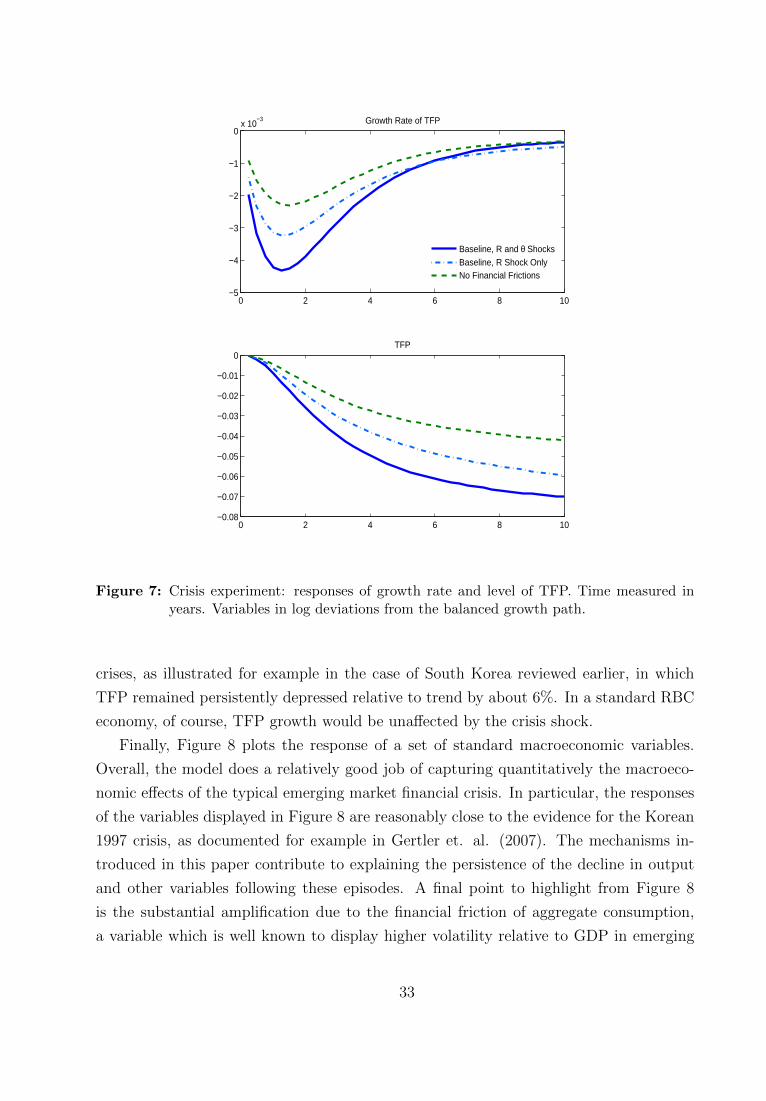
translates into a decline in the rate of newly successful firms. As shown in Figure 7,
it follows that there is a substantial slowdown in the growth rate of TFP, leading to
a permanent drop in the level of this variable relative to the balanced growth path.
Further, the magnitude of the medium-run decline is substantially larger due to financial
factors – in the baseline model, the level of TFP after six years falls more than 6 percent
with both shocks and almost 5 percent with only the interest rate shock, compared to
only 3.5 percent in the model without financial frictions. Thus, the financial friction
plays a quantitatively significant role in helping the model generate a persistent decline
in TFP following a crisis. Such movements in TFP are a salient feature of financial
31
0 2 4 6 8 10
−0.3
−0.2
−0.1
0Successful Firm Value, v
0 2 4 6 8 10
−0.6
−0.4
−0.2
0New Firm Value, J
Baseline, R and θ Shocks
Baseline, R Shock Only
No Financial Frictions
0 2 4 6 8 10−1
−0.5
0
0.5Aggregate Net Worth, W
0 2 4 6 8 10−0.05
0
0.05
0.1
0.15
0.2
E(RZ) − R
0 2 4 6 8 10
0
0.1
0.2
0.3
0.4Multiplier on Incentive Constraint
0 2 4 6 8 10−0.4
−0.3
−0.2
−0.1
0Aggregate bank debt, D
0 2 4 6 8 10−0.25
−0.2
−0.15
−0.1
−0.05
0
Aggregate New Projects, ZN
Figure 6: Crisis experiment: responses of growth and financial intermediation variables. Timemeasured in years. All variables in log deviations from the balanced growth pathexcept net worth, expressed in level deviation as fraction of value in the balancedgrowth path.
32
0 2 4 6 8 10−5
−4
−3
−2
−1
0x 10
−3 Growth Rate of TFP
0 2 4 6 8 10−0.08
−0.07
−0.06
−0.05
−0.04
−0.03
−0.02
−0.01
0TFP
Baseline, R and θ ShocksBaseline, R Shock OnlyNo Financial Frictions
Figure 7: Crisis experiment: responses of growth rate and level of TFP. Time measured inyears. Variables in log deviations from the balanced growth path.
crises, as illustrated for example in the case of South Korea reviewed earlier, in which
TFP remained persistently depressed relative to trend by about 6%. In a standard RBC
economy, of course, TFP growth would be unaffected by the crisis shock.
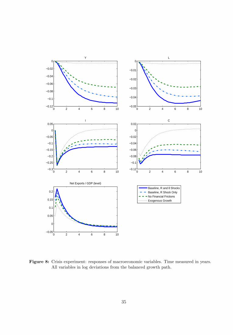
Finally, Figure 8 plots the response of a set of standard macroeconomic variables.
Overall, the model does a relatively good job of capturing quantitatively the macroeco-
nomic effects of the typical emerging market financial crisis. In particular, the responses
of the variables displayed in Figure 8 are reasonably close to the evidence for the Korean
1997 crisis, as documented for example in Gertler et. al. (2007). The mechanisms in-
troduced in this paper contribute to explaining the persistence of the decline in output
and other variables following these episodes. A final point to highlight from Figure 8
is the substantial amplification due to the financial friction of aggregate consumption,
a variable which is well known to display higher volatility relative to GDP in emerging
33
markets when compared to more developed economies, and also of the ratio of net exports
to GDP.
5 Conclusion
This paper has sought to explain the highly persistent effects of financial crises. It has
argued that the phenomenon of slow recoveries from financial crises can be a natural
consequence of an adverse shock in an environment in which productivity growth is en-
dogenous through the creation of new firms. Further, it has shown how domestic financial
market disruptions can work to amplify these declines. Thanks to these mechanisms, the
model developed here is able to quantitatively reproduce the persistent declines in output,
labor productivity and employment following financial crises identified from the data.
The evidence presented in this paper has been based on the experience of emerging
market economies, as have been some of the modeling choices made (for example, the
interest rate shock used to motivate a crisis, or the small open economy assumption).
The reason is that it is in these countries where most financial crises have occurred over
the past decades. The recent wave of financial crises in advanced economies, however,
also appears to display a substantial degree of persistence, and many have suggested a
slowdown in the underlying rate of productivity growth as a possible explanation.34 With
minor adaptation, the mechanisms introduced in this paper could be used to address the
case of advanced economies as well.
A potentially interesting application of the framework presented in this paper would
be an evaluation of the welfare gains of government intervention in mitigating a financial
crisis. Gertler and Karadi (2011) and Gertler, Kiyotaki and Queralto (2012), for example,
analyze different government financial policies in the context of the recent financial crisis
in the US, finding important benefits of government intervention. The endogenous pro-
ductivity growth mechanism introduced in this paper would likely affect what is at stake
when considering intervention during a financial meltdown, and therefore it could have a
substantial impact on the welfare gains of government policies directed at ameliorating
the impact of a crisis.
34See Bernanke (2012) or Section 3 of Bank of England (2012).
34
0 2 4 6 8 10−0.12
−0.1
−0.08
−0.06
−0.04
−0.02
0Y
0 2 4 6 8 10−0.05
−0.04
−0.03
−0.02
−0.01
0L
0 2 4 6 8 10−0.3
−0.25
−0.2
−0.15
−0.1
−0.05
0
0.05I
0 2 4 6 8 10−0.12
−0.1
−0.08
−0.06
−0.04
−0.02
0
0.02C
0 2 4 6 8 10−0.05
0
0.05
0.1
0.15
0.2
Net Exports / GDP (level)
Baseline, R and θ ShocksBaseline, R Shock OnlyNo Financial FrictionsExogenous Growth
Figure 8: Crisis experiment: responses of macroeconomic variables. Time measured in years.All variables in log deviations from the balanced growth path.
35
References
[1] Aoki, K., G. Benigno and N. Kiyotaki (2007). “Capital Flows and Asset Prices,”NBER International Seminar on Macroeconomics 2007
[2] Aguiar, M. and G. Gopinath (2007). “Emerging Market Business Cycles: The CycleIs the Trend,” Journal of Political Economy 115(1), 69-102
[3] Ayyagari, M., A. Demirguc-Kunt and V. Maksimovic (2007) “Firm Innovation inEmerging Markets: The Roles of Governance and Finance,” World Bank Policy Re-search Working Paper 4157
[4] Bank of England (2012). Inflation Report, November 2012
[5] Benhabib, J. and M. Spiegel (1994). “The Role of Human Capital in Economic De-velopment: Evidence from Aggregate Cross-Country Data,” Journal of MonetaryEconomics 34(2), 143-173
[6] Benjamin, D. and F. Meza (2009). “Total Factor Productivity and Labor Realloca-tion: The Case of the Korean 1997 Crisis,”The B.E. Journal of Macroeconomics : Vol.9: Iss.1 (Advances), Article 31
[7] Benhabib, J., R. Rogerson and R. Wright (1991). “Homework in Macroeconomics:Household Production and Aggregate Fluctuations,” Journal of Political Economy99(6), 1166-1187
[8] Bernanke, B. (2012). “The Economic Recovery and Economic Policy,” Speech at theEconomic Club of New York, November 2012
[9] Bernanke, B. and M. Gertler (1989). “Agency Costs, Net Worth, and Business Fluc-tuations,” American Economic Review 79(1), 14-31
[10] Bernanke, B., M. Gertler and S. Gilchrist (1999). “The Financial Accelerator in aQuantitative Business Cycle Framework,” Handbook of Macroeconomics, North Hol-land
[11] Bilbiie, F., F. Ghironi and M. Melitz (2012). “Endogenous Entry, Product Variety,and Business Cycles,” Journal of Political Economy, 120(2), 304-345
[12] Calvo, G. (1998). “Capital Flows and Capital-Market Crises: The Simple Economicsof Sudden Stops,” Journal of Applied Economics, I(1), 35-54
[13] Caprio, G. and D. Klingebiel (2003). “Episodes of Systemic and Borderline FinancialCrises,” mimeo
[14] Cerra, V. and S. C. Saxena (2008). “Growth Dynamics: The Myth of EconomicRecovery,” American Economic Review 98(1), 439-457
[15] Chari, V. V., Kehoe, P. and E. McGrattan (2008). “Business Cycle Accounting,”Econometrica 75(3), 781-836
36
[16] Coe, D., E. Helpman and A. Hoffmaister (2009). “International R&D Spillovers andInstitutions,” European Economic Review 53(7), 723-741
[17] Comin, D. and M. Gertler (2006). “Medium-Term Business Cycles,” American Eco-nomic Review 96(3), 523-551
[18] Comin, D., M. Gertler and A. Santacreu (2009). “Technology Innovation and Diffu-sion as Sources of Output and Asset Price Fluctuations,” mimeo
[19] Comin, D., N. Loayza, F. Pasha and L. Serven (2009). “Medium-Term Cycles inDeveloping Countries,” mimeo
[20] Del Negro, M., G. Eggertsson, A. Ferrero and N. Kiyotaki (2010)“The Great Escape?A Quantitative Evaluation of the Fed’s Non-Standard Policies,” mimeo
[21] Galı, J., M. Gertler and D. Lopez-Salido (2007), “Markups, Gaps, and the WelfareCosts of Business Fluctuations,” Review of Economics and Statistics 89(1), 44-59
[22] Gertler, M., S. Gilchrist and F. Natalucci (2007). “External Constraints on MonetaryPolicy and the Financial Accelerator,” Journal of Money, Credit and Banking 39(2-3),295-330
[23] Gertler, M. and P. Karadi (2011). “A Model of “Unconventional” Monetary Policy,”Journal of Monetary Economics 58, 17-34
[24] Gertler, M. and N. Kiyotaki (2010). “Financial Intermediation and Credit Policy inBusiness Cycle Analysis,” Handbook of Monetary Economics Vol.3, 547-599
[25] Gertler, M., N. Kiyotaki and A. Queralto (2012). “Financial Crises, Bank RiskExposure and Government Financial Policy,” Journal of Monetary Economics 59,S17-S34
[26] Gopinath, G. and B. Neiman (2011). “Trade Adjustment and Productivity in LargeCrises,” American Economic Review, forthcoming
[27] Gorodnichenko, Y. and M. Schnitzer (2010). “Financial Constraints and Innovation:Why Poor Countries Don’t Catch Up,” Journal of the European Economic Associa-tion, forthcoming
[28] Greenwood, J., Z. Hercowitz and G. W. Huffman (1988). “Investment, CapacityUtilization and the Real Business Cycle,” American Economic Review 78, 402-417
[29] Griliches, Z. (1990). “Patent Statistics as Economic Indicators: A Survey,” Journalof Economic Literature XXVIII (December 1990), 1661-1707
[30] Hall, R. (1997). “Macroeconomic Fluctuations and the Allocation of Time,” Journalof Labor Economics 15(1), S223-50
[31] Hall, B. (2002). “The Financing of Research and Development,” Oxford Review ofEconomic Policy, 18(1): 35-51
37
[32] Hall, B. and J. Lerner (2009). “The Financing of R&D and Innovation,” NBERWorking Paper No. 15325
[33] Howard, G., R. Martin and B. A. Wilson (2011). “Are Recoveries from Bankingand Financial Crises Really So Different?,” International Finance Discussion PaperNumber 1037
[34] International Monetary Fund (2009). World Economic Outlook, October 2009 Edi-tion
[35] Jaimovich, N. and S. Rebelo (2009).“Can News about the Future Drive the BusinessCycle?,” American Economic Review 99(4), 1097-1118
[36] Jaffe, A. B. and M. Trajtenberg (2002).“Patents, Citations and Innovations: AWindow on the Knowledge Economy,” Cambridge, MA: MIT Press
[37] Jermann, U. and V. Quadrini (2012).“Macroeconomic Effects of Financial Shocks,”American Economic Review 102(1), 238-271(34)
[38] Kalemli-Ozcan, S., B. Sorensen and S. Yesiltas (2012). “Leverage across firms, banks,and countries” Journal of International Economics 88, 284-289
[39] Kehoe, T. and K. Ruhl (2009).“Sudden stops, sectoral reallocations, and the realexchange rate,” Journal of Development Economics 89(2), 235-249
[40] Kerr, W. and R. Nanda (2009). “Democratizing entry: Banking deregulations, fi-nancing constraints, and entrepreneurship” Journal of Financial Economics 94, 124-149
[41] Kiyotaki, N. and J. Moore (1997). “Credit Cycles,” Journal of Political Economy105(2), 211-248
[42] Kiyotaki, N. and J. Moore (2012). “Liquidity, Business Cycles and Monetary Policy,”mimeo
[43] Kortum, S. and J. Lerner (2000). “Assessing the contribution of venture capital toinnovation,” RAND Journal of Economics 31(4), 674-692
[44] Krueger, A. and J. Yoo (2001). “Chaebol Capitalism and the Currency-FinancialCrisis in Korea,” NBER Conference on Currency Crises Prevention
[45] Laeven, L. and F. Valencia (2012). “Systemic Banking Crises Database: An Up-date,” IMF Working Paper
[46] Levine, R. (1997). “Financial Development and Economic Growth: Views andAgenda,” Journal of Economic Literature 35(2), 688-726
[47] Levine, R. (2005). “Finance and Growth: Theory and Evidence,” in P. Aghion andS. Durlauf, eds: Handbook of Economic Growth (North-Holland Elsevier Publishers,Amsterdam)
38
[48] Mansfield, E., M. Schwartz and S. Wagner (1981). “Imitation Costs and Patents:An Empirical Study,” The Economic Journal 91, 907-918
[49] McGrattan, E. and E. Prescott (2010). “Technology Capital and the US CurrentAccount,” American Economic Review 100(4): 1493-1522
[50] Mendoza, E. (2010). “Sudden Stops, Financial Crises, and Leverage” American Eco-nomic Review 100(5): 1941-1966
[51] Mendoza, E. and V. Z. Yue (2012). “A General Equilibrium Model of SovereignDefault and Business Cycles,” Quarterly Journal of Economics 127(2): 889-946
[52] Meza, F. and E. Quintin (2007). “Factor Utilization and the Real Impact of FinancialCrises,” The B.E. Journal of Macroeconomics : Vol. 7: Iss.1 (Advances), Article 33
[53] Neumeyer, P. A. and F. Perri (2005). “Business Cycles in Emerging Economies: TheRole of Interest Rates,” Journal of Monetary Economics 52, 345-380
[54] Pakes, A. and M. Schankerman (1984). “The Rate of Obsolescence of Knowledge,Research Gestation Lags, and the Private Rate of Return to Research Resources,”pp. 73-88 in Z. Griliches (Ed.),Patents, R&D and Productivity, The University ofChicago Press
[55] Pratap, S. and C. Urrutia (2010). “Financial Frictions and Total Factor Productivity:Accounting for the Real Effects of Financial Crises,” Review of Economic Dynamics,15(3) 336-358
[56] Reinhart, C. M. and V. R. Reinhart (2010) “After the Fall,”NBER Working Paper16334
[57] Reinhart, C. M. and K. S. Rogoff (2009) “This Time is Different: Eight Centuriesof Financial Folly,” Princeton University Press
[58] Romer, P. (1990). “Endogenous Technological Change,” Journal of Political Econ-omy 98(5), 71-102
[59] Uribe, M. and V. Z. Yue (2006). “Country Spreads and Emerging Countries: WhoDrives Whom?,” Journal of International Economics 69, 6-36
[60] Young, A. (1995). “The Tyranny of Numbers: Confronting the Statistical Realitiesof the East Asian Growth Experience,” Quarterly Journal of Economics 110(3): 641-680
39
Appendix
A Data
Data on real output and employment (in number of persons) are obtained from the Total
Economy Database.35 The data on employment used is broadly consistent with the
employment dataset in Neumeyer and Perri (2005) for the set of countries used in that
analysis. Systemic banking crisis episode dates are from Laeven and Valencia (2012).
The list of countries and episodes used in the analysis is the following (episode start-
ing date in parenthesis): Indonesia (1997), Malaysia (1997), Korea (1997), Thailand
(1983, 1997), Philippines (1983, 1997), Argentina (1980, 1989, 1995, 2001), Brazil (1990,
1994), Chile (1976, 1981), Colombia (1982, 1998), Mexico (1981, 1994), Peru (1983), Is-
rael (1977), Poland (1990), Turkey (1982, 2000), Hungary (1991, 2008), Czech Republic
(1996), Slovak Republic (1998).
B Complete Set of Equilibrium Conditions
B.1 Households and Firms
Yt = A1
ϑ−1
t (utKt)αL1−α
t (B.1)
UC,t = uC,t − βhEt (uC,t+1) (B.2)
uC,t =
(Ct − hCt−1 − Γt
1
1 + εL1+εt
)−ρ(B.3)
uC,tΓtLεt
UC,t=
1
1 + θW
(Rt−1Rt
)(1− α)YtLt
(B.4)
Λt,t+1 =βUC,t+1
UC,t(B.5)
1 = Et (Λt,t+1)Rt (B.6)
1 = βEt
(Λt,t+1
α Yt+1
Kt+1+ PK,t+1 − δ(ut+1)
PK,t
)(B.7)
35http://www.conference-board.org/data/economydatabase/
40
Et−1(PK,t) = Et−1
[Φ′(IntKt
)]−1
(B.8)
Int = It − δ(ut)Kt (B.9)
Kt+1 = Kt + Φ
(IntKt
)Kt (B.10)
αYtut
= δ′(ut)Kt (B.11)
1
RtBt −Bt−1 + Yt = Ct + It +Nt (B.12)
Rt = r + ert + ψ
[eBt−BYt − 1
](B.13)
B.2 Entrepreneurs and Financial Intermediaries
πt =1
ϑ
YtAt
(B.14)
vt = πt + φAEt(Λt,t+1vt+1) (B.15)
RZ,t = φZλvt + (1− λ)Jt
Jt−1(B.16)
Wt = σ [(RZ,t −Rt−1) Jt−1St−1 +Rt−1Wt−1] + (1− σ)ξJt−1St−1 (B.17)
Jt [φZ (Zt + ZN,t)−At] = φtWt (B.18)
Ωt = 1− σ + σ (νt + φtµt) (B.19)
µt = Et [Λt,t+1Ωt+1 (RZ,t+1 −Rt)] (B.20)
νt = Et (Λt,t+1Ωt+1)Rt (B.21)
φt =νt
θ − µt(B.22)
41
At+1 = λ [φZ (Zt + ZN,t)−At] + φAAt (B.23)
Zt+1 = φZ (Zt + ZN,t) (B.24)
Jt =1
η
(1
LS
) 1−ηη(ZN,tAt
) 1−ηη
(B.25)
Nt = ηZN,tJt (B.26)
In the frictionless benchmark, equations (B.17)-(B.21) become irrelevant, and instead per-
fect arbitrage holds:
Jt = Et Λt,t+1φZ [λvt+1 + (1− λ)Jt+1] (B.27)
The model is solved by first appropriately detrending the variables that exhibit long-
run growth, in order to obtain a stationary system. The steady state of that system
characterizes the balanced growth path of the economy. Dynamics are obtained by com-
puting a loglinear approximation around the balanced growth path.
C Effects of Non-financial Shocks
Here I analyze the behavior of the model economy following two types of non-financial
shocks that have been highlighted in the literature as important sources of business cycle
fluctuations: an exogenous TFP shock, and a wage markup shock. To introduce the
former, I modify the production function of intermediate goods firms as follows:
Yt(s) = At [ut(s)Kt(s)]α Lt(s)
1−α (C.1)
Above, At is an exogenous aggregate TFP shock. To introduce the wage markup
shock, the labor supply equation is modified according to the following:
Wt = µWtuC,tΓtL
εt
UC,t(C.2)
µWt is a markup of the wage over the household’s marginal disutility of work. Several
authors have argued that countercyclical movements in the wage markup are an impor-
42
tant source of business fluctuations,36 possibly by capturing in a reduced-form way the
effects of nominal price and wage rigidities or labor market frictions.
Figures 9 and 10 report the effects of a 5% decline in exogenous TFP and a 5%
increase in the wage markup, respectively. Both shocks persist as an AR(1) with a 0.95
coefficient. The key point to note is that both shocks induce only modest declines in the
endogenous component of TFP, and that the degree of amplification through the credit
market imperfection is also relatively small. The reason is that unlike financial shocks,
these two types of shocks induce modest movements in the asset prices vt and Jt. As a
consequence, both the frictionless effect on firm creation is small (since the movement
in vt is relatively small) and also the degree of amplification due to financial frictions is
small, since the relatively modest movements in asset prices lead to only mild fluctuations
in banks’ net worth. Further, in the case of wage markup shocks, labor productivity does
not decline – in fact it slightly increases initially due to the sharp drop in employment.
As the figures illustrate, these types of disturbances are followed by a recovery, which is
driven by the unwinding of the shock. Thus, the bottomline from Figures 9 and 10 is
that the model is also consistent with the evidence that especially deep and persistent
output losses are a phenomenon especially associated with recessions involving financial
crises, as Reinhart and Rogoff (2009) and others have noted.
36See Hall (1997), Galı, Gertler and Lopez-Salido (2007) and Chari, Kehoe and McGrattan (2007).
43
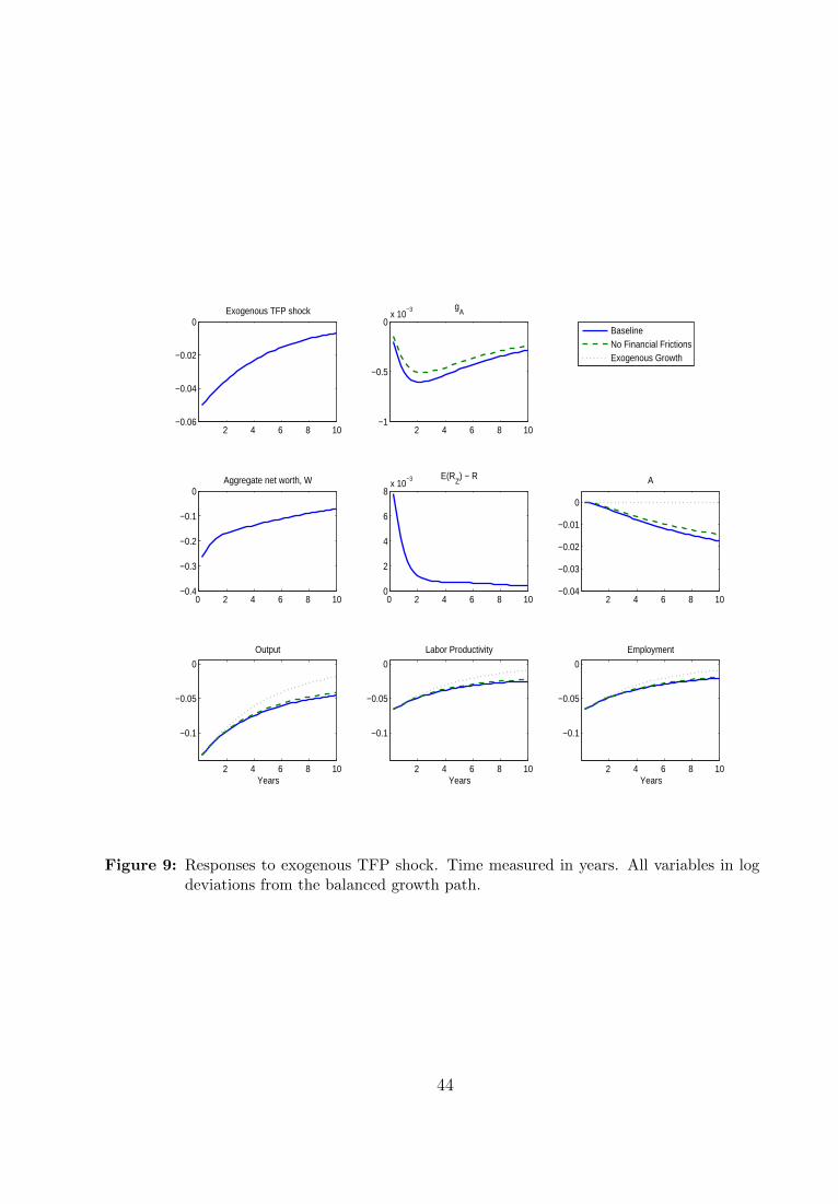
2 4 6 8 10−0.06
−0.04
−0.02
0Exogenous TFP shock
2 4 6 8 10−1
−0.5
0x 10
−3 gA
0 2 4 6 8 10−0.4
−0.3
−0.2
−0.1
0Aggregate net worth, W
0 2 4 6 8 100
2
4
6
8x 10
−3 E(RZ) − R
2 4 6 8 10−0.04
−0.03
−0.02
−0.01
0
A
2 4 6 8 10
−0.1
−0.05
0
Output
Years2 4 6 8 10
−0.1
−0.05
0
Labor Productivity
Years2 4 6 8 10
−0.1
−0.05
0
Employment
Years
BaselineNo Financial FrictionsExogenous Growth
Figure 9: Responses to exogenous TFP shock. Time measured in years. All variables in logdeviations from the balanced growth path.
44
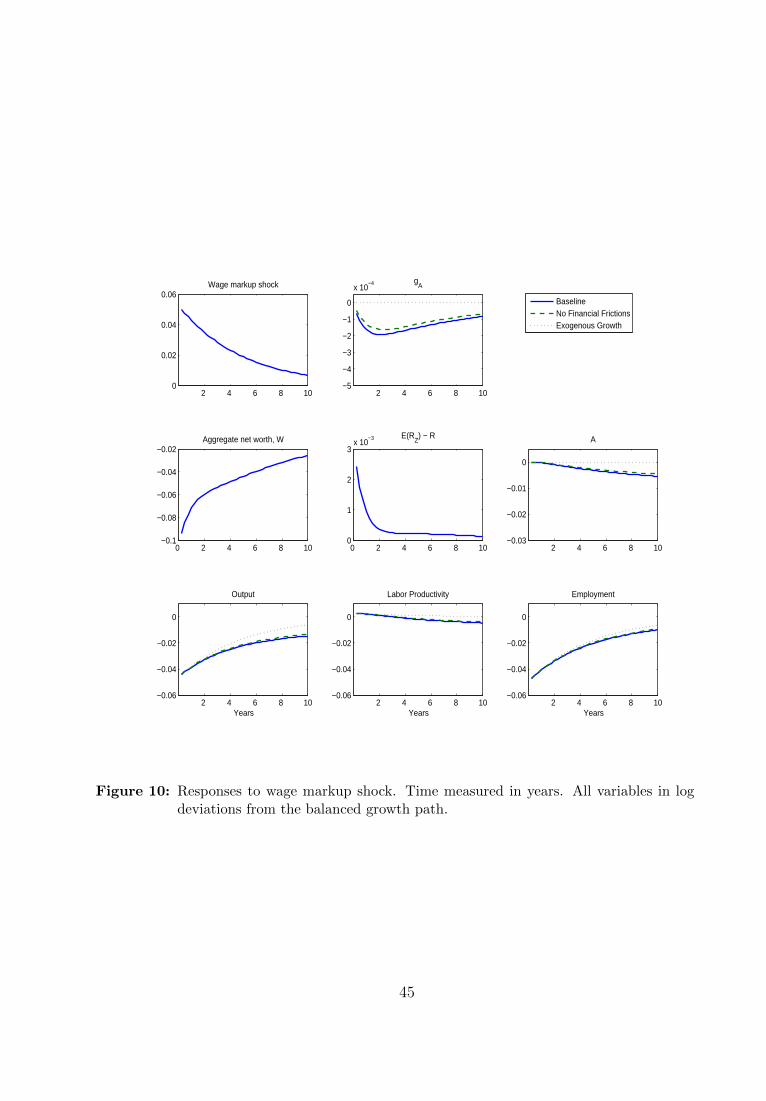
2 4 6 8 100
0.02
0.04
0.06Wage markup shock
2 4 6 8 10−5
−4
−3
−2
−1
0
x 10−4 g
A
0 2 4 6 8 10−0.1
−0.08
−0.06
−0.04
−0.02Aggregate net worth, W
0 2 4 6 8 100
1
2
3x 10
−3 E(RZ) − R
2 4 6 8 10−0.03
−0.02
−0.01
0
A
2 4 6 8 10−0.06
−0.04
−0.02
0
Output
Years2 4 6 8 10
−0.06
−0.04
−0.02
0
Labor Productivity
Years2 4 6 8 10
−0.06
−0.04
−0.02
0
Employment
Years
BaselineNo Financial FrictionsExogenous Growth
Figure 10: Responses to wage markup shock. Time measured in years. All variables in logdeviations from the balanced growth path.
45