a model with a unified kinematic hardening law for cyclic
TRANSCRIPT
*Correspondance to: École des Ponts ParisTech, Laboratoire Navier–CERMES, 6-8 av.
B. Pascal, 77455 Marne-la-Vallée cedex 2, France
Email address: [email protected] (J. M. Pereira)
Preprint submitted to Computers and Geotechnics
A model with a unified kinematic hardening law for cyclic
behavior of stiff clays
P. Y. Honga, J. M. Pereira
a,*, Y. J. Cui
a, A. M. Tang
a, F. Collin
b, X.L. Li
c
aUniversité Paris-Est, Laboratoire Navier (UMR 8205), CNRS, ENPC, IFSTTAR, F-77455 Marne-la-Vallée, France
bDepartment GeomaC, University of Liège, Sart Tilman B52/3, Chemin des Chevreuils, 1, B-4000, Liege, Belgium
cEuropean Underground Research Infrastructure for Disposal of Nuclear Waste in Clay Environment, ESV EURIDICE GIE,
Mol, Belgium.
Abstract: This paper presents a kinematic hardening model for describing some important
features of natural stiff clays under cyclic loading conditions, such as closed hysteretic loops,
smooth transition from the elastic behavior to the elastoplastic one and changes of the
compression slope with loading/unloading loops. The model includes two yield surfaces, an
inner surface and a bounding surface. A non-associated flow rule and a unified kinematic
hardening law are proposed for the inner surface. The adopted hardening law enables the
plastic modulus to vary smoothly when the kinematic yield surface approaches the bounding
surface and ensures at the same time the non-intersection of the two yield surfaces.
Furthermore, the first loading, unloading, and reloading stages are treated differently by
applying distinct hardening parameters. The main feature of the model is that its constitutive
equations can be simply formulated based on the consistency condition for the inner yield
surface based on the proposed unified kinematic hardening law; thereby, this model can be
easily implemented in a finite element code using a classic stress integration scheme as for the
modified Cam Clay model. The simulation results on the Boom Clay, natural stiff clay, have
revealed the relevance of the model: a good agreement has been obtained between simulations
and the experimental results from the tests with different stress paths under cyclic loading
conditions. In particular, the model can satisfactorily describe the complex case of oedometric
conditions where the deviator stress is positive upon loading (compression) but can become
negative upon unloading (extension).
Keywords: natural stiff clay; kinematic hardening; cyclic loading; elastoplasticity; stress
integration; validation
2
1. Introduction
It is well known that the stress-strain curves of soils under cyclic loading conditions show
hysteresis loops with gradual accumulation of permanent strain. Indeed, various experimental
results from isotropic compression tests, drained triaixal shear tests and oedometer tests on
natural stiff clays (Boom Clay and Ypresian Clays, for instance) with several
unloading/reloading cycles show marked hysteresis loops [1, 2, 3]. Natural stiff clays also
exhibit smooth transition from elastic to elastoplastic compression (progressive stiffness
degradation with strain) for either loading or unloading/reloading stages. In addition,
experiments show another important characteristic regarding the compression slope in the
reloading process before reaching ′vmax which is the maximum vertical stress applied before
unloading. This compression slope in the reloading process varies significantly from one loop
to another. Nguyen [4] concluded that this slope increases with ′vmax. These features must be
taken into account when developing constitutive models for the description of the mechanical
behavior of this kind of clays under cyclic loading conditions.
Conventional critical state models for soils including the Modified Cam Clay model (MCC)
can describe plastic strains in the normally consolidated state, but only elastic strains is
produced during the subsequent unloading–reloading cycles within the yield surface. On the
other hand, bounding surface models with radial mapping rule proposed in the 1980s (see e.g.
[5, 6]), where the current plastic modulus varies with the distance between the stress state and
its image point on the bounding surface, can successfully describe some important features of
natural stiff clays such as the smooth transition from elastic to elastoplastic states as well as
the softening behavior. However, this kind of the models gives open hysteresis loops during
unloading-reloading stages and cannot describe the cyclic loading behavior realistically, since
no plastic strain is generated during the unloading process. To overcome this deficiency,
attempts were made by some researchers (e.g. [7, 8]]) by applying the generalized plasticity
concept proposed by Zienkiewicz and Mroz [9]. It is assumed that plastic strain is produced
even by a stress increment directed toward the inside of the yield surface, the stress point
always lying on the inner yield surface. With the generalized plasticity concept, a gradual
strain accumulation with closed hysteresis loops can be simulated for the loading compression
side (the deviator stress is positive). However, it fails for the extension side (negative
deviator stress): an inflection appears in the stress-strain curve upon unloading along a
straight stress path [10] as illustrated in Fig. 1. It is assumed that the loading yield surface has
3
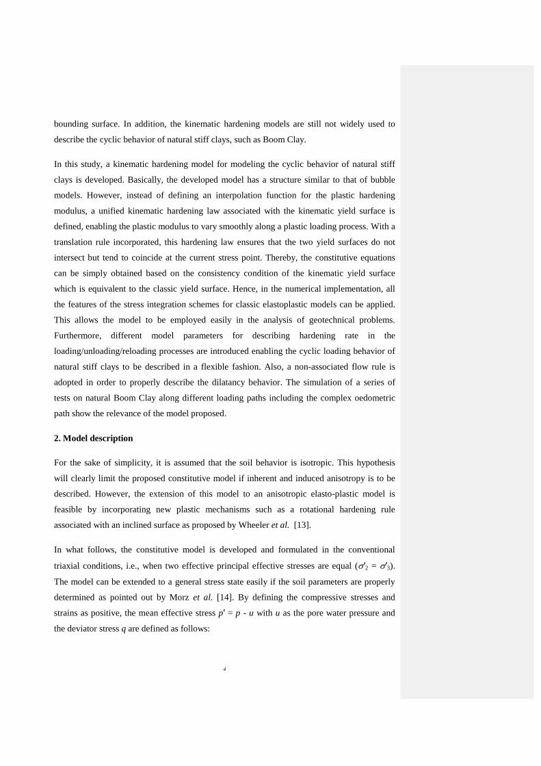
an ellipse shape as in the MCC model (see Fig. 1 (a)). During the unloading process (path 1-2),
the loading surface shrinks from fl1 to fl2 with the size parameter decrease from p′c1 to p′c2. A
negative plastic strain increment is generated for this loading path. When point 3 is reached,
the direction of the effective stress rate becomes tangential to the loading surface and just
elastic strain is produced leading to an inflection point (see Fig. 1 (b)). After point 3, the
loading surface expands along p′ axis passing through the origin of the stress space with a
positive plastic strain increment generated. Indeed, the predicted behavior that a negative
plastic strain increment generated along path 1-3 but a positive plastic strain increment along
path 3-4 is difficult to admit physically. Hence, this kind of the models is not suitable for
simulating the oedometer tests where negative deviator stress occurs in the unloading process.
Fig. 1. Problems related to the bounding surface models with isotropic hardening law considering plastic strain
in the unloading process: (a) the stress path in the (p′, q) plane and (b) the stress-volumetric plastic strain curve
An important development in the constitutive modeling for the cyclic loading behavior is the
introduction of kinematic hardening mechanism by Mroz (1967) [11]. The ‘Bubble’ model by
Al-Tabbaa (1989) [12] was developed within the framework of kinematic models. In this
model, a kinematic yield surface (namely bubble surface) is defined, which is allowed to
translate and expand or contract within the conventional yield surface (namely bounding
surface). The formulation of such a kinematic hardening model is mainly centered on the
translation rule and the hardening function: the former is used to control the movement and
interaction of the two surfaces and the latter is defined to describe the variation of the plastic
modulus. This model can reproduce a closed hysteretic loop under a complete cyclic loading
with deviator stress being from positive values to negative values. However, it should be
pointed out that in the bubble model, the plastic modulus of the current stress state is not
formulated by considering the consistency condition of the kinematic yield surface, but given
by an interpolation function depending on the distance from the current stress point to the
Commentaire [JMP1]: No I do not understand your comments.
4
bounding surface. In addition, the kinematic hardening models are still not widely used to
describe the cyclic behavior of natural stiff clays, such as Boom Clay.
In this study, a kinematic hardening model for modeling the cyclic behavior of natural stiff
clays is developed. Basically, the developed model has a structure similar to that of bubble
models. However, instead of defining an interpolation function for the plastic hardening
modulus, a unified kinematic hardening law associated with the kinematic yield surface is
defined, enabling the plastic modulus to vary smoothly along a plastic loading process. With a
translation rule incorporated, this hardening law ensures that the two yield surfaces do not
intersect but tend to coincide at the current stress point. Thereby, the constitutive equations
can be simply obtained based on the consistency condition of the kinematic yield surface
which is equivalent to the classic yield surface. Hence, in the numerical implementation, all
the features of the stress integration schemes for classic elastoplastic models can be applied.
This allows the model to be employed easily in the analysis of geotechnical problems.
Furthermore, different model parameters for describing hardening rate in the
loading/unloading/reloading processes are introduced enabling the cyclic loading behavior of
natural stiff clays to be described in a flexible fashion. Also, a non-associated flow rule is
adopted in order to properly describe the dilatancy behavior. The simulation of a series of
tests on natural Boom Clay along different loading paths including the complex oedometric
path show the relevance of the model proposed.
2. Model description
For the sake of simplicity, it is assumed that the soil behavior is isotropic. This hypothesis
will clearly limit the proposed constitutive model if inherent and induced anisotropy is to be
described. However, the extension of this model to an anisotropic elasto-plastic model is
feasible by incorporating new plastic mechanisms such as a rotational hardening rule
associated with an inclined surface as proposed by Wheeler et al. [13].
In what follows, the constitutive model is developed and formulated in the conventional
triaxial conditions, i.e., when two effective principal effective stresses are equal (′2 = ′3).
The model can be extended to a general stress state easily if the soil parameters are properly
determined as pointed out by Morz et al. [14]. By defining the compressive stresses and
strains as positive, the mean effective stress p′ = p - u with u as the pore water pressure and
the deviator stress q are defined as follows:
5
1 3 1 3
1p 2 q
3 (1)
where ′1 and ′3 are the axial and lateral effective stresses, respectively.
The volumetric strain v and the shear strain s are defined as:
v 1 3 s 1 32 (2)
where 1 and 3 are the axial and lateral strains, respectively.
2.1. Elastic behavior
As in the MCC, the elastic volumetric strain increment is given by:
e
v
dpd
K
(3)
with the elastic bulk modulus as follows:
0v pK
(4)
where is the elastic slope in a specific volume-logarithmic mean stress plane (v, ln p′) and v0
is the initial specific volume.
The elastic shear strain increment can be calculated by:
e
s
dqd
3G (5)
and the shear modulus G can be calculated with a constant Poisson's ratio ν:
3 1 2 KG
2 1
(6)
It is well-known that this choice for shear modulus (Eq (6)) helps in simulating experimental
results, but leads to thermodynamic inconsistency since the Maxwell symmetry relations are
not satisfied in this case [15, 16].
2.2 Plastic behavior
2.2.1 Yield surfaces
6
Two yield surfaces are introduced (see Fig. 2): an outer yield surface namely bounding
surface (fb) that represents the normal consolidation behavior and an inner kinematic yield
surface (fk) that delimits an elastic domain. The yield behavior is described in terms of
evolutions of the kinematic yield surface within the domain delimited by the bounding surface.
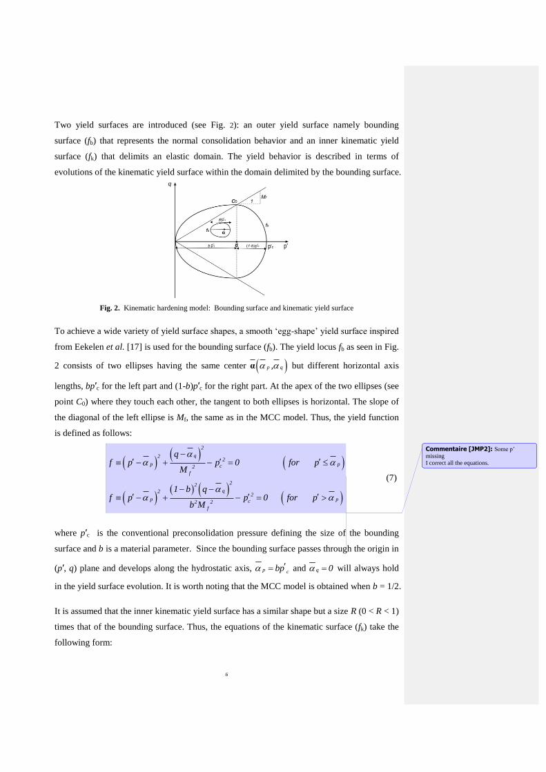
Fig. 2. Kinematic hardening model: Bounding surface and kinematic yield surface
To achieve a wide variety of yield surface shapes, a smooth ‘egg-shape’ yield surface inspired
from Eekelen et al. [17] is used for the bounding surface (fb). The yield locus fb as seen in Fig.
2 consists of two ellipses having the same center α p q, but different horizontal axis
lengths, bp′c for the left part and (1-b)p′c for the right part. At the apex of the two ellipses (see
point C0) where they touch each other, the tangent to both ellipses is horizontal. The slope of
the diagonal of the left ellipse is Mf, the same as in the MCC model. Thus, the yield function
is defined as follows:
2
q22
p pc2
f
22
q22
p pc2 2
f
qf p p 0 for p
M
1 b qf p p 0 for p
b M
(7)
where p′c is the conventional preconsolidation pressure defining the size of the bounding
surface and b is a material parameter. Since the bounding surface passes through the origin in
(p′, q) plane and develops along the hydrostatic axis, p cbp and q 0 will always hold
in the yield surface evolution. It is worth noting that the MCC model is obtained when b = 1/2.
It is assumed that the inner kinematic yield surface has a similar shape but a size R (0 < R < 1)
times that of the bounding surface. Thus, the equations of the kinematic surface (fk) take the
following form:
Commentaire [JMP2]: Some p’ missing I correct all the equations.
7
2
2 2q
p c p2
f
22
2 2q
p c p2 2
f
qf p Rp 0 for p
M
1 b qf p Rp 0 for p
b M
(8)
where α(αp, αq) is the coordinates that specify the position of the center of the kinematic yield
surface.
2.2.2 Isotropic hardening law
The isotropic hardening law is defined to describe the evolution of the bounding surface size
(through parameter p′c) with plastic strains. The evolution of p′c depends on the plastic
volumetric strain p
v as in the MCC model, and is given by:
p0 cc v
v pdp d
(9)
where λ is the normal consolidation slope in (v, ln p′) plane. This isotropic hardening law also
applies implicitly to the kinematic yield surface through the constant ratio R as the kinematic
yield surface is activated.
2.2.3 Kinematic hardening law
Consider now the kinematic hardening law for the kinematic yield surface. The current stress
state is defined as ,σ =T
p q (point A in Fig. 3) which lies on the kinematic surface is
associated with a conjugated stress state σ p ,q (point B in Fig. 3) on the bounding
surface having the same direction of the exterior normal, as illustrated in Fig. 3. The similarity
of the kinematic yield surface and the bounding surface gives the following relationship:
σ α σ αR
(10)
8
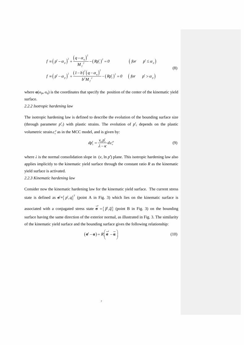
Fig. 3. Schematic representation of the kinematic hardening law
To account for the progressive increment of plastic strain as the kinematic yield surface
approaches the bounding surface, a scalar r measuring the normalized distance of the current
stress state on the kinematic yield surface to the associated conjugated stress state on the
bounding surface is defined as follows:
max
r
(11)
where σ σ is the current distance between the current stress state and the conjugated
stress state, max denotes the maximum distance: max c1 R p . Obviously, r = 0 holds
when the two surfaces are in contact.
A simple law is defined to describe the evolution of r following Borja et al. [18]:
2 p0
d
vdr s r d
(12)
with a generalized plastic strain defined in Eq (13) to account for the contribution of both the
volumetric and shear plastic strains:
2 2
p p p
d v d sd d A d (13)
Commentaire [JMP3]: Add these distances to fig.2
I add them.
9
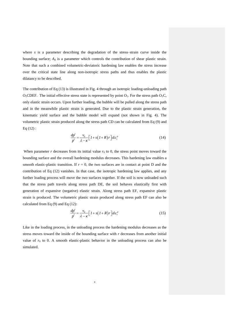
where s is a parameter describing the degradation of the stress–strain curve inside the
bounding surface; Ad is a parameter which controls the contribution of shear plastic strain.
Note that such a combined volumetric-deviatoric hardening law enables the stress increase
over the critical state line along non-isotropic stress paths and thus enables the plastic
dilatancy to be described.
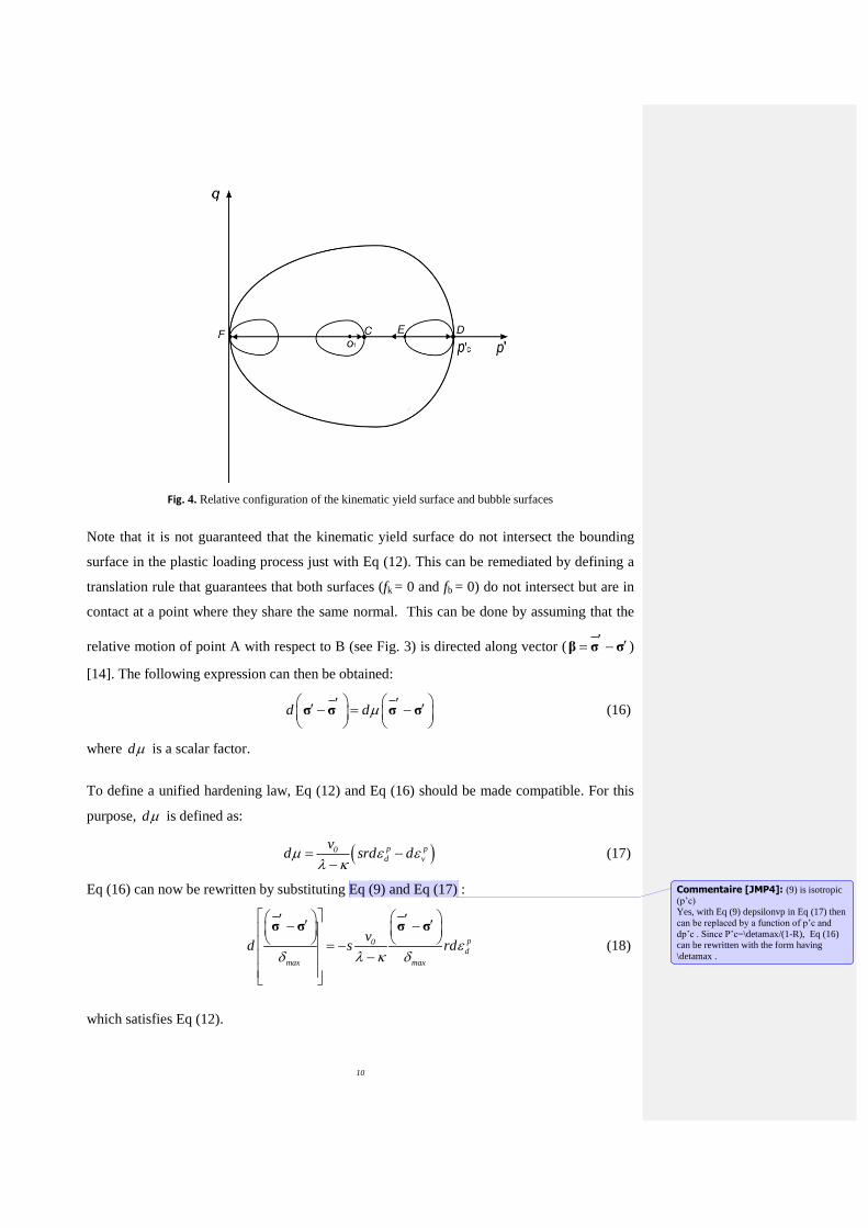
The contribution of Eq (13) is illustrated in Fig. 4 through an isotropic loading-unloading path
O1CDEF. The initial effective stress state is represented by point O1. For the stress path O1C,
only elastic strain occurs. Upon further loading, the bubble will be pulled along the stress path
and in the meanwhile plastic strain is generated. Due to the plastic strain generation, the
kinematic yield surface and the bubble model will expand (not shown in Fig. 4). The
volumetric plastic strain produced along the stress path CD can be calculated from Eq (9) and
Eq (12) :
p0v
vdp1 s 1 R r d
p
(14)
When parameter r decreases from its initial value r0 to 0, the stress point moves toward the
bounding surface and the overall hardening modulus decreases. This hardening law enables a
smooth elastic-plastic transition. If r = 0, the two surfaces are in contact at point D and the
contribution of Eq (12) vanishes. In that case, the isotropic hardening law applies, and any
further loading process will move the two surfaces together. If the soil is now unloaded such
that the stress path travels along stress path DE, the soil behaves elastically first with
generation of expansive (negative) elastic strain. Along stress path EF, expansive plastic
strain is produced. The volumetric plastic strain produced along stress path EF can also be
calculated from Eq (9) and Eq (12):
p0v
dp v1 s 1 R r d
p
(15)
Like in the loading process, in the unloading process the hardening modulus decreases as the
stress moves toward the inside of the bounding surface with r decreases from another initial
value of r0 to 0. A smooth elastic-plastic behavior in the unloading process can also be
simulated.
10
Fig. 4. Relative configuration of the kinematic yield surface and bubble surfaces
Note that it is not guaranteed that the kinematic yield surface do not intersect the bounding
surface in the plastic loading process just with Eq (12). This can be remediated by defining a
translation rule that guarantees that both surfaces (fk = 0 and fb = 0) do not intersect but are in
contact at a point where they share the same normal. This can be done by assuming that the
relative motion of point A with respect to B (see Fig. 3) is directed along vector (β σ σ )
[14]. The following expression can then be obtained:
σ σ σ σd d
(16)
where d is a scalar factor.
To define a unified hardening law, Eq (12) and Eq (16) should be made compatible. For this
purpose, d is defined as:
p p0d v
vd srd d
(17)
Eq (16) can now be rewritten by substituting Eq (9) and Eq (17) :
σ σ σ σp0
d
max max
vd s rd
(18)
which satisfies Eq (12).
Commentaire [JMP4]: (9) is isotropic (p’c)
Yes, with Eq (9) depsilonvp in Eq (17) then
can be replaced by a function of p’c and
dp’c . Since P’c=\detamax/(1-R), Eq (16) can be rewritten with the form having
\detamax .
11
Substituting the geometric relation given by Eq (10) into Eq (18) gives a unified kinematic
hardening law:
α σ σ σ α αp p0d v
c
c
1vs
R dpd dr
pdd
R
(19)
This kinematic hardening law specifies the translation of the centre of the kinematic yield
surface and enables the plastic modulus to vary at the same time, having a unified function of
the hardening law and the translation rule in a classic kinematic hardening model.
2.2.4 Hardening parameter s and loading cycles
To satisfactorily describe the closed hysteretic loop behavior, a well-known solution is to
divide the whole cyclic loading process into three parts, namely first loading, unloading and
reloading processes (e.g. [19, 20]). For each part, a specific expression of plastic modulus is
used to control the corresponding slope of the stress-strain curve. Following this concept,
parameters s0, su and sr are introduced to control the hardening rate for the first loading,
unloading and reloading processes, respectively.
Furthermore, as mentioned before, an important behavior regarding slope Ccp in the reloading
process before reaching ′vmax (the maximum vertical stress applied before unloading) has
been observed experimentally: Ccp varies significantly from one loop to the next one. For
Boom Clay and Ypresian Clays, oedometer tests have revealed that Ccp varies linearly with
the logarithm of ′vmax [4]. Since K0 (the coefficient of earth pressure at rest) is close to 1 for
natural Boom Clay (K0 = 0.80) and Ypresian Clays (K0 = 0.88) [21, 22], the vertical effective
stress state can then be approximated by the mean effective stress. Therefore, the following
expression can be adopted for hardening parameter sr :
rr 0 s
max
ps s log
p
(20)
where λs is a material constant which controls the variation rate of sr; p′r is the initial mean
effective stress in the reloading process; p′max is the maximum mean effective stress applied
before unloading. This equation ensures that the higher the value of p′max or the lower the
value of p′r, the lower the value of sr, thus the straighter the stress-strain curve for the
reloading before reaching p′max (or ′vmax).
2.2.5 Flow rule
Commentaire [JMP5]: Don’t you have a problem with the sign of \sigma-
\bar\sigma
I am sorry that I don’t see the problem. This is the classic equation describing geometric
similarities of the two surfaces. Could you
please explain the problem in more detail?
Commentaire [JMP6]: Why do you call it unified. This is not clear
This kinematic hardening law, unlike in a
classic kinematic hardening model, has a unified function of hardening law and
translation rule. I want to highlight this
characteristic. So I call it unified hardening
law. Do you think it is necessary to name it?
If it does, do you have an appropriate word?
12
In the common critical state models, the phenomenological interaction between shear and
volume change (contraction and dilatancy) has been well handled by specifying an
appropriate flow rule. In the well-known MCC model, the flow rule is defined as follows:
2 2pgv
p
s
Md
d 2
(21)
where is the stress ratio q/p′; Mg is the critical state slope corresponding to the stress ratio
when there is no further volumetric strain. In the loading process, if gM , plastic
compression occurs; if gM , plastic dilatancy occurs.
If an associated plastic flow rule is adopted in this model, it gives
2pp fv
pp
s q
2 2pp fv
p2p
s q
p Mdfor p
d q
p b Mdfor p
d 1 b q
(22)
where f gM M holds in the associated flow rule.
It can be clearly seen that the contractive plastic phase, dilative phase and the critical state
controlled by Eq (22) depends on the relative position between the current effective stress
state and the center of kinematic yield surface, instead of the value of gM as in the MCC
model. Hence, a non-associated flow rule is defined by modifying the associated flow rule
expressed by Eq (22) :
when loading/reloading
when unloading
pg p cv
p
s g q c
pg p cv
p
s g q c
M 2 p 2 Rpd
d k 2 q Rp
M 2 p 2 Rpd
d k 2 q Rp
(23)
where kg is a material constant that is used to control the magnitude of the ratio of plastic
volumetric strain increment to plastic shear strain increment. During loading, the sign of Eq
(23) is controlled by the value of gM . This value allows distinguishing the plastic
contractive phase, plastic dilative phase and the critical state. Similarly, during unloading, Eq
(23) defines the plastic contractive phase, the plastic dilative phase, and the critical state when
gM , gM and gM , respectively.
Commentaire [JMP7]: Unclear I rewrite this part.
13
2.5 Constitutive equations
In the following, the equations for the plastic strain increment are formulated by considering
the consistency condition for the kinematic yield surface. The formulations are given in
triaxial {p', q} space. The stress and strain variables write as follows:
, , ,σ εT T
v sp q (24)
The plastic strain increment is computed from the plastic potential as follows:
εσ
p gd d
(25)
where dλ is a positive scalar namely plastic multiplier; g is the plastic potential.
α and p′c act as hardening variables. Therefore, the consistency condition of the kinematic
yield surface is given by:
: σ + : α+σ α
T T
k k kc
c
f f fd d dp 0
p
(26)
Substituting Eqs (9), (19) and (25) into Eq (26) gives:
: σσ
t
kf d hd 0
(27)
with h being the hardening modulus:
σ σ σ α
α
2 2
0d c
T
k
0
c
c
1 Rfh
R
f v g
p
v g g g g gsr A bp
p q p p p
p
p
(28)
From Eq (28), we can see that even when the stress state reaches the condition = Mg, the
inclusion of the shear hardening part (g
q
> 0) leads to h > 0. With further loading, the
effective stress increases over the critical state line and negative plastic volumetric strain
occurs.
The stress-strain equations can finally be obtained in a differential form:
Commentaire [JMP8]: Be careful: you mix triaxial stress space and tensor form while \sigma is also used for the translation
rule and has another meaning
Yes, I mixed them. To simply solve this problem, I re-defined the stress strain
variable (\sigma and \epsilon) and give the
constitutive equations in triaxial space.
Commentaire [JMP9]: ‘ missing
p’_c instead of p’_0
f_k instead of f I correct them.
14
σ D εepd d (29)
where:
b a DD D D
a D b
T e
ep e e
T e h
(30)
and De is the elastic stiffness matrix, a
σ
kf, b
σ
g
.
3. Determination of parameters
The proposed kinematic hardening model has 13 parameters (λ, , p′c0, ν, Mg, R, Mf, b, kg, s0,
su, λs, Ad). The procedure for determining these parameters is described as follows.
1. λ, , p′c0, ν, Mg are common parameters in the MCC model. λ is the slope of the normal
consolidation compression line and is the slope of swelling line of the isotropic
compression curve in (v, ln p′) plane. Note that is the parameter governing the elastic
behavior. However, the proposed kinematic model assumes a purely elastic behavior only
inside the kinematic yield surface in the initial stage of the loading/unloading/reloading
processes. To be consistent with this elasto-plastic framework, can be determined by the
swelling curve in the early stage of the unloading process. p′c0 denotes conventional
isotropic preconsolidation pressure and it defines the initial size of the bounding surface.
These three parameters (λ, and p′c0) can be determined based on the isotropic compression
curve in the (v, ln p′) plane. The Poisson’s ratio ν can be determined from a standard triaxial
test by considering the elastic behavior at a low strain level (around 0.5%) in the (v, 1)
plane: 1 / 2v . Mg is the critical state stress ratio which can be determined by the
effective stress ratio at critical state.
2. R is the ratio of sizes of kinematic yield surface and bounding surface. The size of the
kinematic yield surface is defined by R. Considering its physical meaning, this size can be
determined in the early loading/unloading stage of isotropic compression test, based on the
compression curve in the (v-ln p′) plane.
3. Mf and b are parameters specifying the shape of the yield surface and can be calibrated by
fitting the bounding yield surface shape to the conventional yield points obtained from the
tests of different stress paths.
15
4. kg is used in the plastic flow rule and can be determined by the values of
p p
v sd / d obtained from drained triaxial shear tests.
5. Parameters s0 and su determine the hardening rate for the first loading and unloading,
respectively. λs is a material constant which controls the variation of the hardening rate in
the reloading process. These three parameters can be back calibrated from an isotropic
compression or oedometer test with at least two full unloading/reloading cycles.
4. Prediction and validation
In this section, the performance of the proposed model is assessed by simulating different
tests on natural Boom Clay. This clay was taken in the Underground Research Laboratory
(URL) at Mol, at a depth of 223 m. At this depth, the total vertical stress is around 4.5 MPa
and the pore pressure is equal to 2.2 MPa, defining an effective vertical stress around 2.3 MPa
[23]. As mentioned before, the value of K0 being about 0.8, the initial effective stress state can
be approximated by an isotropic one. As indicated by some researchers ([1, 24, 25]),
saturating samples under low effective stresses induce significant swelling and the subsequent
mechanical tests may not be representative of the behavior of natural Boom clay in field
conditions. Therefore, only data obtained from the tests on samples saturated under the in-situ
effective stress are considered in this study. The results that are taken into account include
those from isotropic compression tests, drained triaixal shear tests and oedometer tests,
carried out in different laboratories.
All the simulations are performed from a common point (p′0 = 2 MPa, e0 = 0.61) which is
assumed to be on the initial kinematic yield surface. Parameters λ, and p′c0 were determined
from the isotropic compression tests; kg, Ad and ν were calibrated using the experimental
curves v-1 from two drained triaxial shear tests; Mf, kf, b and Mg were derived from the
conventional yield stresses and the critical stress ratio of all the drained triaxial shear tests; s0,
su and λs were calibrated from the oedometer test results. These parameters are presented in
Table 1.
Table 1 Model parameters for natural Boom Clay
λ ν p′c0
(MPa) R Mf b
0.18 0.02 0.3 6 0.15 0.7 0.65
Mg kg s0 su λs Ad
0.67 0.14 40 14 10.3 0.2
16
4.1 Isotropic compression test
Many isotropic compression tests on natural Boom Clay samples have been performed and
some of them are summarized in Table 2 [1, 4, 26].
Table 2 Summary of the isotropic tests reported in literature
Test Reference Sample depth (m) Initial void ratio Void ratio after
saturation
Iso-1 Baldi et al. [1]
223
0.677 -
Iso-2 Le [26] 0.620 0.590
Iso-3 Nguyen [4] - 0.600
After completion of the saturation process, isotropic compression was performed under
drained conditions: in Iso-1, the sample was loaded isotropically up to a mean effective stress
of 4 MPa and then unloaded to 2 MPa, reloaded to 8 MPa, unloaded again to 2 MPa, and
reloaded again to 5 MPa; in test Iso-2, the sample was loaded isotropically up to a mean
effective stress of 10 MPa and then unloaded to 2 MPa; in test Iso-3, the sample was loaded
isotropically up to 20 MPa and then unloaded to 0.5 MPa. The volumetric strains were
obtained from the volume of drained-out water in all the three tests.
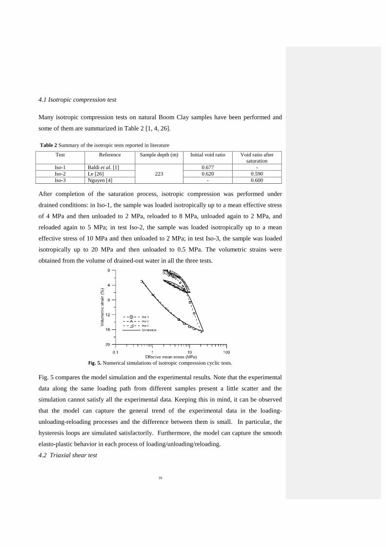
Fig. 5. Numerical simulations of isotropic compression cyclic tests.
Fig. 5 compares the model simulation and the experimental results. Note that the experimental
data along the same loading path from different samples present a little scatter and the
simulation cannot satisfy all the experimental data. Keeping this in mind, it can be observed
that the model can capture the general trend of the experimental data in the loading-
unloading-reloading processes and the difference between them is small. In particular, the
hysteresis loops are simulated satisfactorily. Furthermore, the model can capture the smooth
elasto-plastic behavior in each process of loading/unloading/reloading.
4.2 Triaxial shear test
17
The drained triaxial tests under cyclic loadings performed by Baldi et al. [1] are summarized
in Table 3. These three tests CD-1 and CD-2 and CD-3 are performed under strain-controlled
conditions. Strain reversals were applied at 0.60% and 2.80% of axial strains for CD-1 (Fig.
6), at 0.56% and 2.93% of axial strains for CD-2 (Fig.7), at 0.60% and 3.80% of axial strains
for CD-3 (Fig.8), respectively.
Table 3 Summary of the drained triaxial tests reported in literature.
Test Sample depth
(m)
Water content
(%)
Mean effective stress
before shearing
(MPa)
Initial void ratio Shear rate
(μm/min)
CD-1
223
25.8 2 0.705
1 CD-2 25.8 3 0.717
CD-3 25.7 4 0.712
Figs. 6-8 present a comparison between the experimental results and those predicted by the
model for the drained triaxial tests. The results are presented in terms of variations of deviator
stress and volumetric strain versus axial strain.
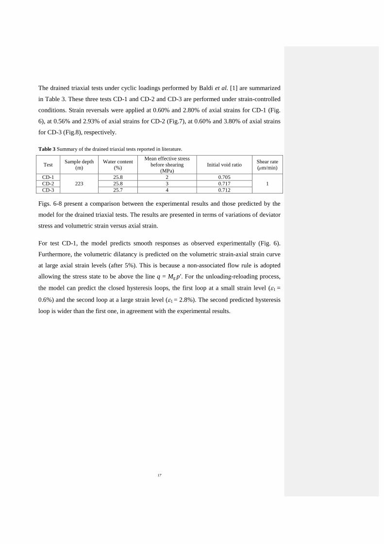
For test CD-1, the model predicts smooth responses as observed experimentally (Fig. 6).
Furthermore, the volumetric dilatancy is predicted on the volumetric strain-axial strain curve
at large axial strain levels (after 5%). This is because a non-associated flow rule is adopted
allowing the stress state to be above the line q = Mg p′. For the unloading-reloading process,
the model can predict the closed hysteresis loops, the first loop at a small strain level (1 =
0.6%) and the second loop at a large strain level (1 = 2.8%). The second predicted hysteresis
loop is wider than the first one, in agreement with the experimental results.
18
Fig. 6. Numerical simulations of drained triaxial shear cyclic test CD-1 (p′0 = 2.0 MPa).
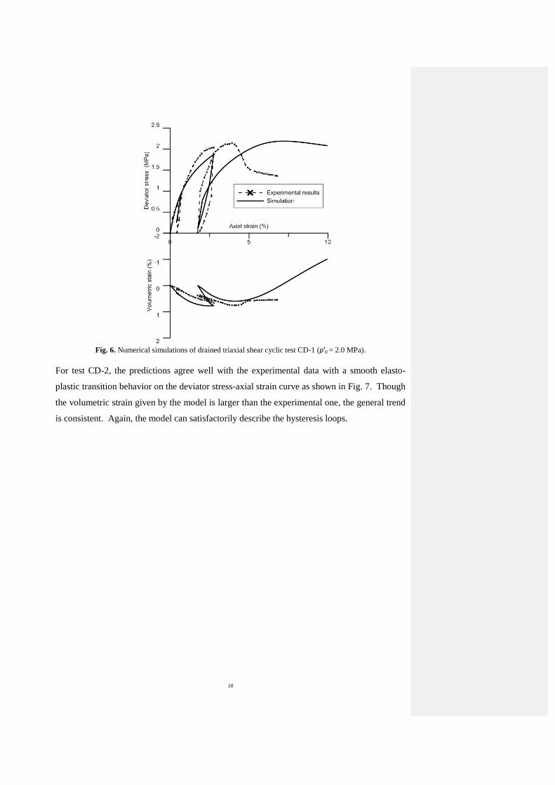
For test CD-2, the predictions agree well with the experimental data with a smooth elasto-
plastic transition behavior on the deviator stress-axial strain curve as shown in Fig. 7. Though
the volumetric strain given by the model is larger than the experimental one, the general trend
is consistent. Again, the model can satisfactorily describe the hysteresis loops.
19
Fig. 7. Numerical simulations of drained triaxial shear cyclic test CD-2 (p′0 = 3.0 MPa).
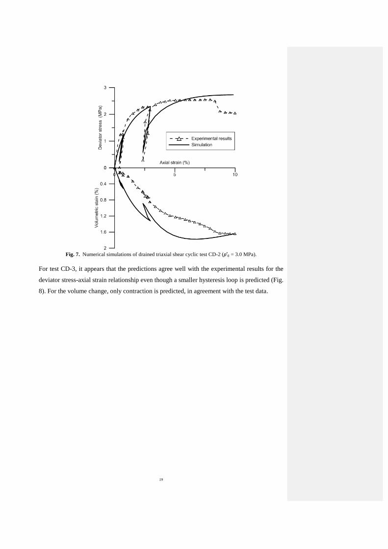
For test CD-3, it appears that the predictions agree well with the experimental results for the
deviator stress-axial strain relationship even though a smaller hysteresis loop is predicted (Fig.
8). For the volume change, only contraction is predicted, in agreement with the test data.
20
Fig. 8. Numerical simulations of drained triaxial shear cyclic test CD-3 (p′0 = 4.0 MPa).
4.3 Oedometer tests
The oedometer tests conditions reported in literature are summarized in Table 4 [1, 3, 27].
Table 4 Summary of the odometer tests reported in literature.
Test Reference Sample depth
(m) Initial void ratio
Void ratio
after saturation
Oed-1 Horseman et al. [3] 247 - 0.608
Oed-2 Deng et al. [27] 223
0.610 0.580
Oed-3 Baldi et al. [1] 0.696-0.717 -
In Oed-1 and Oed-2, the samples were saturated under a vertical effective stress of 1 MPa and
no obvious swelling was found in the saturation process. Compression cycles were then
applied, under the vertical effective stresses of 2, 8, 1, 32 and 1 MPa in Oed-1 and of 2, 16,
0.2, 32, and 0.1 MPa in Oed-2. In Oed-3, the sample was saturated under a higher vertical
effective stress of 2.3 MPa. It was then loaded under 2 and 10 MPa effective vertical stresses.
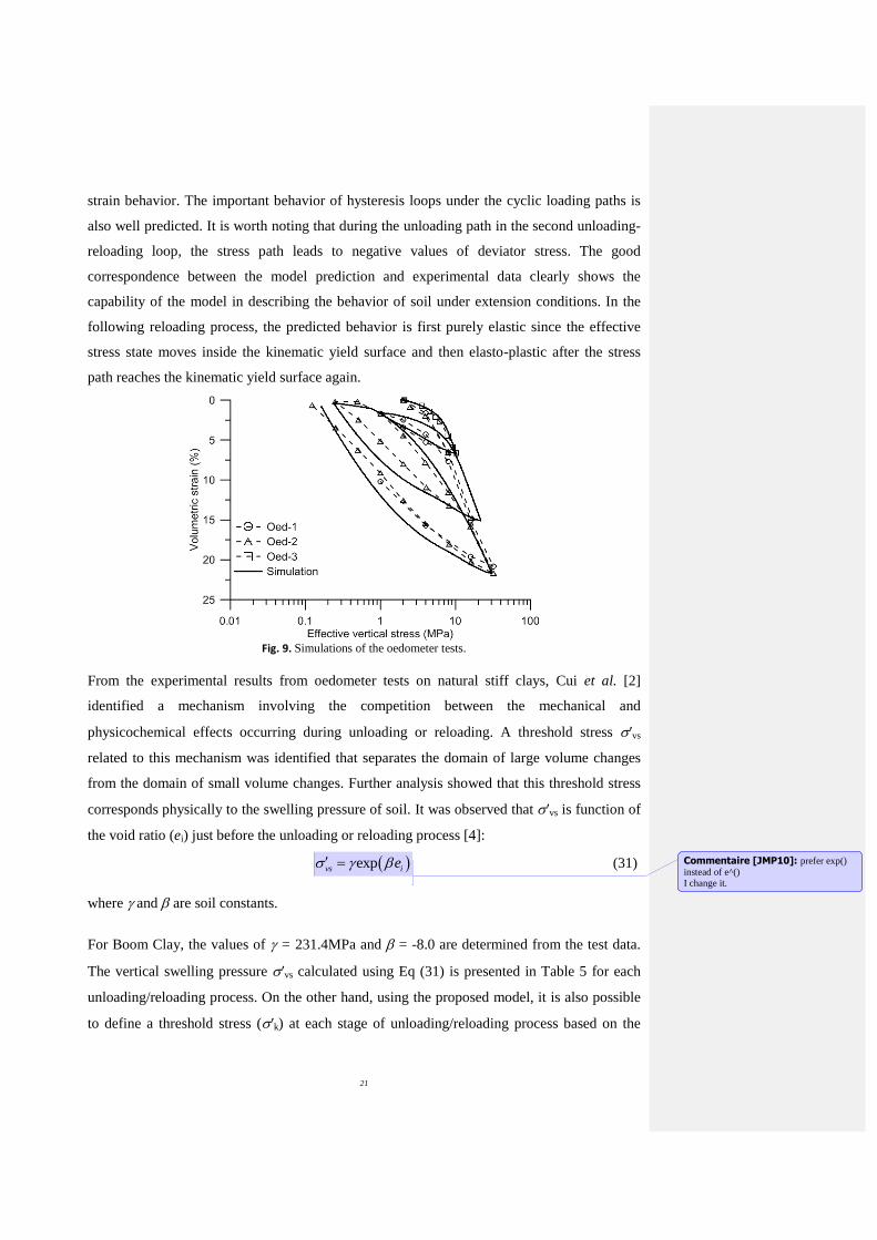
Fig. 9 shows the comparison between the model predictions and the experimental data. It can
be observed clearly that the simulation curves agree well with the experimental ones for each
part of the loading paths, indicating the performance of the model in simulating smooth stress-
21
strain behavior. The important behavior of hysteresis loops under the cyclic loading paths is
also well predicted. It is worth noting that during the unloading path in the second unloading-
reloading loop, the stress path leads to negative values of deviator stress. The good
correspondence between the model prediction and experimental data clearly shows the
capability of the model in describing the behavior of soil under extension conditions. In the
following reloading process, the predicted behavior is first purely elastic since the effective
stress state moves inside the kinematic yield surface and then elasto-plastic after the stress
path reaches the kinematic yield surface again.
Fig. 9. Simulations of the oedometer tests.
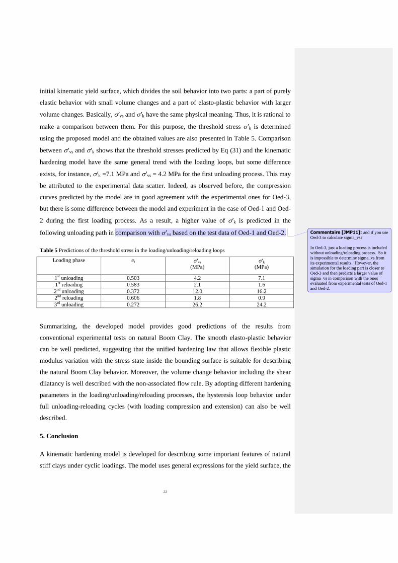
From the experimental results from oedometer tests on natural stiff clays, Cui et al. [2]
identified a mechanism involving the competition between the mechanical and
physicochemical effects occurring during unloading or reloading. A threshold stress ′vs
related to this mechanism was identified that separates the domain of large volume changes
from the domain of small volume changes. Further analysis showed that this threshold stress
corresponds physically to the swelling pressure of soil. It was observed that ′vs is function of
the void ratio (ei) just before the unloading or reloading process [4]:
expvs ie (31)
where and are soil constants.
For Boom Clay, the values of = 231.4MPa and = -8.0 are determined from the test data.
The vertical swelling pressure ′vs calculated using Eq (31) is presented in Table 5 for each
unloading/reloading process. On the other hand, using the proposed model, it is also possible
to define a threshold stress (′k) at each stage of unloading/reloading process based on the
Commentaire [JMP10]: prefer exp()
instead of e^() I change it.
22
initial kinematic yield surface, which divides the soil behavior into two parts: a part of purely
elastic behavior with small volume changes and a part of elasto-plastic behavior with larger
volume changes. Basically, ′vs and ′k have the same physical meaning. Thus, it is rational to
make a comparison between them. For this purpose, the threshold stress ′k is determined
using the proposed model and the obtained values are also presented in Table 5. Comparison
between ′vs and ′k shows that the threshold stresses predicted by Eq (31) and the kinematic
hardening model have the same general trend with the loading loops, but some difference
exists, for instance, ′k =7.1 MPa and ′vs = 4.2 MPa for the first unloading process. This may
be attributed to the experimental data scatter. Indeed, as observed before, the compression
curves predicted by the model are in good agreement with the experimental ones for Oed-3,
but there is some difference between the model and experiment in the case of Oed-1 and Oed-
2 during the first loading process. As a result, a higher value of ′k is predicted in the
following unloading path in comparison with ′vs based on the test data of Oed-1 and Oed-2.
Table 5 Predictions of the threshold stress in the loading/unloading/reloading loops
Loading phase ei ′vs
(MPa)
′k
(MPa)
1st unloading 0.503 4.2 7.1
1st reloading 0.583 2.1 1.6
2nd
unloading 0.372 12.0 16.2
2nd
reloading 0.606 1.8 0.9
3rd
unloading 0.272 26.2 24.2
Summarizing, the developed model provides good predictions of the results from
conventional experimental tests on natural Boom Clay. The smooth elasto-plastic behavior
can be well predicted, suggesting that the unified hardening law that allows flexible plastic
modulus variation with the stress state inside the bounding surface is suitable for describing
the natural Boom Clay behavior. Moreover, the volume change behavior including the shear
dilatancy is well described with the non-associated flow rule. By adopting different hardening
parameters in the loading/unloading/reloading processes, the hysteresis loop behavior under
full unloading-reloading cycles (with loading compression and extension) can also be well
described.
5. Conclusion
A kinematic hardening model is developed for describing some important features of natural
stiff clays under cyclic loadings. The model uses general expressions for the yield surface, the
Commentaire [JMP11]: and if you use
Oed-3 to calculate sigma_vs?
In Oed-3, just a loading process is included without unloading/reloading process. So it
is impossible to determine sigma_vs from
its experimental results. However, the simulation for the loading part is closer to
Oed-3 and then predicts a larger value of
sigma_vs in comparison with the ones evaluated from experimental tests of Oed-1
and Oed-2.
23
MCC yield surface being a special case. A unified kinematic hardening law associated with
the kinematic yield surface is introduced, enabling the plastic modulus to vary flexibly when
the kinematic yield surface approaches the bounding surface. The kinematic surface can be in
contact with the bounding surface but never intersect with it. The non-associated flow rule
adopted allows the shear and volume change behavior to be satisfactorily described,
especially the shear dilatancy behavior. In addition, by introducing three model parameters for
describing the hardening rate in the first loading/unloading/reloading process, the cyclic
loading behavior of natural stiff clays can be flexibly modeled. With the unified hardening
law introduced, the constitutive equations of the model can be simply formulated based on the
consistency condition for the kinematic yield surface. Therefore, the proposed kinematic
hardening model can be easily implemented in a numerical code using a stress integration
scheme as for the MCC model.
Comparisons between the model predictions and the experiment data from the tests on natural
Boom Clay show that the model is capable to capture the overall stress-strain behavior along
different loading paths under cyclic loading conditions. In particular, the model can
satisfactorily describe the complex case of oedometer tests where the deviator stress can
become negative during unloading.
Acknowledgements
The authors are grateful to the Chinese Scholar Council and the Euridice/Ondraf for their
financial supports.
Reference:
[1] G. Baldi, T. Hueckel, A. Peano, R. Pellegrini, Developments in modelling of thermo-
hydro-geomechanical behaviour of boom clay and clay-based buffer materials, Commission
of the European Communities, Nuclear Science and Technology (1991) EUR 13365/1 and
EUR 13365/2.
[2] Y. J. Cui, X. P. Nguyen, A. M. Tang, X. L. Li, An insight into the unloading/reloading
loops on the compression curve of natural stiff clays, Applied Clay Science 83 (2013) 343–
348.
24
[3] S. Horseman, M. Winter, D. Entwistle, Geotechnical characterization of boom clay in
relation to the disposal of radioactive waste, Final report, EUR 10987. Luxembourg:
Commission of the European Communities.
[4] X. P. Nguyen, Étude du comportement chimico-hydro-mécanique des argiles raides
dans le contexte du stockage de déchets radioactifs, Ph.D. thesis, Université Paris-Est, France
(2013).
[5] Y. Dafalias, L. Herrmann, A bounding surface soil plasticity model, in: International
Symposium on Soils under Cyclic and Transient Loading, Swansea, UK, Vol. 1, 1980, pp.
335–345.
[6] Y. Dafalias, Bounding surface plasticity. i: Mathematical foundation and
hypoplasticity, Journal of Engineering Mechanics 112 (9) (1986) 966–987.
[7] H. Hirai, An elastoplastic constitutive model for cyclic behaviour of sands,
International journal for numerical and analytical methods in geomechanics 11 (5) (1987)
503–520.
[8] C. Aboim, W. Roth, Bounding surface plasticity theory applied to cyclic loading of
sand, in: International Symposium on Numerical Models in Geomechanics, 1982, pp. 65–72.
[9] O. Zienkiewicz, Z. Mroz, Generalized plasticity formulation and applications to
geomechanics, Mechanics of engineering materials (1984) 655–679.
[10] K. Hashiguchi, Z.-P. Chen, Elastoplastic constitutive equation of soils with the
subloading surface and the rotational hardening, International Journal for Numerical and
Analytical Methods in Geomechanics 22 (3) (1998) 197–227.
[11] Z. Mroz, On the description of anisotropic workhardening, Journal of the Mechanics
and Physics of Solids 15 (3) (1967) 163–175.
[12] A. Al Tabbaa, D. M. Wood, An experimentally based bubble model for clay, in:
Proceedings of the 3rd International Symposium on Numerical Models in Geomechanics
(NUMOG III), Elsevier, 1989, pp. 90–99.
[13] S. Wheeler, A. Naatanen, M. Karstunen, M. Lojander, An anisotropic elastoplastic
model for soft clays, Canadian Geotechnical Journal 40 (2) (2003) 403–418.
[14] Z. Mroz, V. Norris, O. Zienkiewicz, The application of an anisotropic hardening
model in the analysis of elasto-plastic deformation of soils, Geotechnique 29 (1).
[15] G. Houlsby, A. Puzrin, Principles of hyperplasticity: an approach to plasticity theory
based on thermodynamic principles, Springer, 2006.
25
[16] M. Zytynski, M. Randolph, R. Nova, C. Wroth, On modelling the unloading-reloading
behaviour of soils, International Journal for Numerical and Analytical Methods in
Geomechanics 2 (1) (1978) 87–93.
[17] S. J. van Eekelen, P. van den Berg, The delft egg model, a constitutive model for clay,
in: DIANA Computational Mechanics ’94, Springer, 1994, pp. 103–116.
[18] R. Borja, C. Lin, F. Montáns, Cam-clay plasticity, part iv: Implicit integration of
anisotropic bounding surface model with nonlinear hyperelasticity and ellipsoidal loading
function, Computer methods in applied mechanics and engineering 190 (26-27) (2001) 3293–
3323.
[19] H. S. Yu, C. Khong, J. Wang, A unified plasticity model for cyclic behaviour of clay
and sand, Mechanics Research Communications 34 (2) (2007) 97–114.
[20] C. Hu, H. Liu, W. Huang, Anisotropic bounding-surface plasticity model for the cyclic
shakedown and degradation of saturated clay, Computers and Geotechnics 44 (2012) 34–47.
[21] A. F. L. Amorim, Thermo-hydro-mechanical behaviour of two deep belgium clay
formations: Boom and ypresisan clay, Ph.D. thesis, Universitat Politècnica de Catalunya,
Spain (2011).
[22] S. Horseman, M. Winter, D. Entwisle, Triaxial experiments on boom clay,
Enginnering Geology Special Publication (1993) 35–35.
[23] F. Bernier, X. L. Li, W. Bastiaens, Twenty-five years’ geotechnical observation and
testing in the tertiary boom clay formation, Géotechnique 57 (2) (2007) 229–237.
[24] P. Delage, T. T. Le, A. M. Tang, Y. J. Cui, X. L. Li, Suction effects in deep boom clay
block samples, Géotechnique 57 (1) (2007) 239–244.
[25] P. Y. Hong, Development and explicit integration of a thermo-mechanical model for
saturated clays, Ph.D. thesis, Université Paris-Est, France (2013).
[26] T. Lê, Comportement thermo-hydro-mécanique de l’argile de boom, Ph.D. thesis,
École Nationale des Ponts et Chaussées (2008).
[27] Y. F. Deng, A. M. Tang, Y. J. Cui, X. P. Nguyen, X. L. Li, L. Wouters, Laboratory
hydro-mechanical characterisation of boom clay at essen and mol, Physics and Chemistry of
the Earth, Parts A/B/C 36 (17) (2011) 1878–1890.