UNIVERSITY OFILLINOIS LIBRARY

AT URE3 IA-CHAMPAIGN3COK3TACK5

Faculty Working Papers

College of Commerce and Business Administration

University of Illinois at U r ba n a - C h a m pa I g n

ic is also consistent with Leibenstcin' s notion that chill

ml commitment goods in terms of time and money.

Changes in contraceptive technology seem to be important il

ig births. The increase in the power of the technology hasj

Lble for households to more realistically examine children

;work postulated by the Chicago School, Leibonstein, or Easl

FACULTY WORKING PAPERS

College of Commerce and Business Administration

University of Illinois at Urbana-Champaign

April 26, 1979

A MULTIVARIATE ANALYSIS OF ANNUAL EARNINGS

FORECASTS GENERATED FROM QUARTERLY FORECASTS OFFINANCIAL ANALYSTS AND UNIVARIATE TIME SERIES

MODELS

William S. Hopwood, Assistant ProfessorsDept.

of AccountancyWilliam A. Collins, University of Florida

#561

SUMMARY:

The study compares the forecast accuracy of financial analysts, ARIMA

models, and various permier models considered in the literature in the

predicting of annual earnings per share. Various refinements were made of

previously used methodologies. The results of the multivariate analysis

indicated that financial analysts provide the most accurate forecasts.

In additions the divergence in accuracy between the various sources

of forecasts tend to decrease as the end of the year approaches, while

at the same time there is a general increase in accuracy. Also specific

results are provided for individual model performance.

Digitized by the Internet Archive

in 2011 with funding from

University of Illinois Urbana-Champaign

http://www.archive.org/details/multivariateanal561hopw

A Multivariate Analysis of Annual

Earnings Forecasts Generated from OuarterlyForecasts of Financial Analysts and

Univariate Time Series Models

There is a widespread belief that the use of forecasted accounting

earnings as a measu-e of expected earnings power is of primary impor-

tance in investment decisions. The Financial Accounting Standards

Board [1977] recently reir, forced this belief in their conceptual frame-

work project. A major question, however, exists as to the most appro-

priate source of these forecasts. Current sources widely available are

financial analysts and univariate time series models. Folicy making

loards, such as the SEC and the FASB, are considering whether these '

sources are ade ]uate or whether managotnent also should be required to

forecast accounting earning. Since empirical researchers that have

investigated aspects of Investment decisions, such as cost of capital,

firrc valuation, ard the relationships between earnings and stock

prices, have utilized forecasted accounting earnings as their measure

of oarni.gs ^; pectations, they also should be concerned with an evalua-

tion of fcrocist sourcss.

Because of t'.-.c difficulties of specifying a complete operational

ationship between the forecast source and the investment decision,

includirg a loss function, previous research that attempted to evaluate

the ccn,petir.^ icurces of forecast information generally has focused on

a stated or implied purpose of these forecasts. The purpose considered

in this ra?er is the ability to predict annual earnings from quarterly

forecasts. Thic purpose has been suggested in the discussion memoran-

dum , InterJ-n Financial Accounting and Reporting (FASB fl978l); it also

i "- • ':•:..- i

nas been the subject of previous research. Most of these related

-2-

research studies did not incorporate the more sophisticated time series

analysis currently available. The more current study by Lorek [1979]

compared the predictive ability of four univariate time series models

as well as certain more naive models; his comparison, however, did not

include financial analysts.

In addition, these studies generally utilized univariate statis-

tical methods when the multiple model and multiple time period factors

indicated that a multivariate hypothesis was being considered. Several

problems are raised by the use of univariate methods. First, the uni-

variate approach to the research issue necessitates a larger number of

tests of the null hypothesis rather than a single multivariate test.

Since each individual test has an associated alpha error, there is a

greater possibility that a number of these tests will reject the null

hypothesis purely by chance. An additional problem relates to the

assumption that univariate tests conducted at multiple time periods on

the forecasted earnings for the same firms are independent. Since earn-

ings variables for the same firm usually are highly correlated, the

univariate tests may not be independent. These problems of combined

reliability and statistical dependence may have affected the empirical

findings and the resultant conclusions.

The present study considers these problems while providing a com-

parison of the relative accuracy of annual earnings forecasts generated

from the quarterly forecasts of financial analysts and the four uni-

variate time series models evaluated by Lorek [1979]. This comparison,

however, is provided based on a multivariate analysis of variance de-

sign (MANOVA). The MANOVA was chosen, because, as a multivariate test,

-3-

it provides the advantage of overcoming the problems of combined relia-

bility and statistical dependence, finally the multivariate procedure

is very powerful (Cooly and Lohnes, 1971, p. 228) and as used in the

present study is virtually distribution free. The MANOVA model is

described in detail in a subsequent section.

In addition, the univariate models were reidentified and reestimated

as each earnings figure in the test period was announced. Unlike most

previous studies, then, this study utilized all earnings data that was

available at the time a forecast was generated. This is considered

potentially very important because comparing two models based on fore-

cast errors when one model is based on more up to date information might

produce a bias in favor of the more up to date model.

Finally the present study differs from previous research in that

the parametric testing allows a consideration of the magnitude of the

data in testing. This provides for information not available via the

rise of non-parametric ranking procedures. In fact, forecast methods

might be identical in their average ranking of forecast errors but

quite different with respect to their simple means.

The paper is organized into four major sections. An analysis of

the methodologies and results relating to prior research in the area is

presented first in order to provide justification for the models chosen

in the present study. The research design and statistical tests uti-

lized in the present study then are presented followed by the empirical

results. A summary of these results and the conclusions obtained com-

plete the presentation.

-4-

PREVIOIIS RESEARCH RESULTS

Univariate Models

The four univariate models are generated utilizing the time series

2process suggested by Box and Jenkins [1970], The complete process is

a statistical technique that is used to (a) identify, in a parsimonious

manner, the most appropriate model consistent with the apparent under-

lying process that generated the observed time service data; (b) esti-

mate the parameter values for that particular model; and (c) perform

diagnostic tests. The process consists of an iterative approach that

excludes inappropriate models until the model and its parameter values

that best fit the data are selected. Compared to previous time series

analyses that were characterized by the individual consideration of

many possible models, the Box and Jenkins process permits consideration

of a much greater number of models in a more structured approach.

The first univariate model employed in this study, hereafter desig-

nated the BJ model, is a model individually identified and its para-

meter values estimated for each firm in the study. Thus, the BJ model

for each firm is determined from the complete Box and Jenkins process.

Since the model is determined from the consideration of a broad gener-

alized model inclusive of all possible combinations of autoregressive

and moving average models, the initial expectation might be that fore-

casts generated from an individually fitted model should be more

accurate than forecasts generated from a model that vas generally iden-

tified for all firms. However, the identification process is both

subjective and costly. In addition, the identification of a model from

i

a finite series of data points may not result in the model consistent

v;ith the underlying process generating an infinite series.

-5-

Because of these factors and observed empirical results, it has

been suggested that a generally identified or premier model, v;ith indi-

vidual firm estimation of parameter values may generate forecasts that

are equal or superior to those generated by the BJ model. If a single

model form generates results that are comparable to an individually

identified model, it vould obviate the need to perform the subjective

and costly identification process required for the latter model. It

also v;ould diminish the problem associated fcith the identification of

a model from a finite series of observations.

The models that previously have been proposed are (1) a consecu-

tively and seasonally differenced first order moving average and

seasonal moving average model (Griffin [1977] and Watts [1975]), (2)

a seasonally differenced first order autoregressive model with a con-

stant drift term (Foster [1977]), and (3) a seasonally differenced

first order autoregressive and seasonal moving average model (Brov;n

and Rozeff [1978]). In the notation used by Box and Jenkins, these

models are designated as (0,1,1) X (0,1,1), (1,0,0) X (0,1,0) and

(1,0,0) X (0,1,1), respectively. In this study, they are referred to

3as the GW, F and BR models. The models are generally identified for

all firms with individual firm estimation of the parameter values.

Thus, only the parameter estimation portion of the complete Box and

Jenkins process is used.

The different forms of a single or premier model form have been

suggested based on the diagnostic tests incorporated in the Box and

Jenkins process and also on predictive evidence. Watts, uho initially

suggested a premier model, based this suggestion on evidence that the

average cross-sectional autocorrelation function (acf) could be modeled

-6-

by the (0,1,1) X (0,1,1) model. Griffin also demonstrated that the

average acf could be modeled by the (0,1,1) X (0,1,1) model. His sug-

gestion also was prompted by the consistency of the distribution of

the Box-Pierce statistic with the existence of white noise residuals.

Foster based his suggested model primarily on the evidence that one-

quarter ahead absolute percentage errors associated with the F model

were lower than these errors generated by the BJ model. However, Brown

and Rozeff , Griffin, and Foster himself, note that the F model does not

fit the data in that the model fails to incorporate a systematic sea-

sonal lag. Based on the Foster research, Brown and Rozeff proposed a

model that incorporated a seasonal moving average component and con-

cluded that their model performed favorably against the BJ, F and GW

models over several forecast horizons. Most recently, Lorek [1979] ex-

tended this comparison among these four univariate models by analyzing

their relative ability to predict annual earnings generated from quar-

terly forecasts. His results indicated that as fewer quarterly fore-

casts were included in the annual forecast, the univariate time series

models performed better than more simplistic models. However, based

on the inconsistency of his results and the previous studies by Brown

and Rozeff, Foster, Griffin, and Watts, he concluded that it may be

premature to conclude that a single premier model is best for quarterly

earnings. Thus, the forecast accuracy comparison of the individually

identified and the suggested premier models remains an unanswered ques-

tion.

Financial Analysts Model

In addition to the four univariate model forecasts, the study

included forecasts generated by financial analysts. The univariate

-7-

models can be criticized in that they neglect additional publicly

available information that may be potentially useful; financial ana-

lysts are not subject to this criticism. Rather, financial analysts

have been criticized in that their analysis process may be too de-

tailed and the additional cost incurred may not be justified.

Empirical results that support these assertions v;ere provided by

Cragg and Malkiel [1969] and F.lton and Gruber [1972], Both studies

concluded that analysts' forecasts uere not more accurate than fore-

casts based on earnings streams alone. ' The study by Broun and Rozeff

[1978], on the other hand, led to the conclusion that financial

analysts' forecasts vere superior to forecasts generated solely

from earnings data. These results, however, have been questioned by

Abdel-khalik and Thompson [1977-78] as being overstated due to their

temporal nature. The empirical results, therefore, are inconclusive..

In addition, the relative accuracy of annual earnings forecasts gener

ated from the analysts' quarterly forecasts has not been compared

with similar forecasts from the BJ, BR, F and GW models.

In the present study, these univariate models were included in

order to assess the relative accuracy of these forecasts. Relative

accuracy then may be useful in determining the existence of a premier

model. The results of the univariate models in Comparison to the

financial analysts may be used to provide evidence as to \chether the

additional cost incurred by financial analysts is justified. This

evidence provided as to the relative accuracy of forecasts generated

from earnings data alone and earnings data plus other variables also

may provide useful information to the SEC and the FASB as to the

desirability of management forecast disclosure.

-8-

RESEARCH DESIGN

General Hypothesis

The preceding sections highlight the recent attention given to the

question of whether a single generally applied univariate model pro-

vides equal or superior forecasting results than an individual firm

identified model. An additional question is whether a univariate model

provides equal or superior forecasting results to those of a model that

incorporates more potentially useful information. These questions are

incorporated in the following null and alternative hypothesis.

Hypothesis:

Ho: There is no difference in the forecast error generatedby each of five models (BJ, BR, F, FA and GW)

.

Ha: There is a difference in the forecast error generatedby each of five models (BJ, BR, F, FA and GW)

.

Tto forecast error metrics were calculated. The first metric was

the mean absolute percentage forecast error (MAPFE) which is specified

as:

it itn|

Aiti

where A = actual earnings per share for firm i in quarter t

P. = predicted earnings per share for firm i in quarter t,

generated by model n

This metric was selected because it is a measure that establishes

relative comparability of forecast errors between firms that produce

earnings per share that are different in absolute scale. Since equal

-9-

weight is assigned to all forecast errors it assumes a linear loss

function. However, because of the possibility that outliers might not

be best represented by a linear loss function, an outlier adjusted mean

absolute percentage forecast error metric (OAMAPFE) also was utilized.

This adjustment consisted of assigning the value of 3.0 to all fore-

cast errors that had a value greater than 3.0. The resultant error

metric then assumed a linear loss function that was truncated for out-

liers.

The Multivariate Design

The test of the null hypothesis was based on a multivariate ana-

lysis of variance design (MANOVA). MANOVA is a simple generalization

of analysis of variance (ANOVA). The primary difference is that ANOVA

tests for differences between means for a single variable where MANOVA

tests for difference between means for a group (vector) of variables.

The basic design used in the present study is that of orthogonal

polynomial analysis of doubly multivariate data as described in Bock

(1975, Ch. 7). The approach is one of converting a univariate repeated

measure design into a MANOVA design. In terms of the present research,

it would be possible to consider the forecast model, the quarter from

which the forecast is made, and the year of the forecasts as repeated

measure factors. However this would require the necessity of making

highly restrictive assumptions with respect to the distribution of the

data. The orthogonal polynomial MANOVA eliminates the need to make

these assumptions. In fact the only assumption needed in the present

study is that of multivariate normality and this has been proven to be

-10-

satisfied for sufficiently large samples, via the multivariate central

limit theorem [Anderson, 1958; Harris, 1975, p. 232; Ito, 1969). (The

sample in this research is based on annual forecasts originating in each

of the 20 quarters during the 5 year test period for 50 firms giving

1000 origin dates for each model.) Also, there is typically a need to

make an assumption of equality of subgroup covariance matrices, but this

is not necessary in the present study since the tests involve only one

sample and therefore do not depend on pooling of covariance matrices.

Sample of Firms

The sample of 50 firms (Appendix) were selected randomly from 205

calendar year-end firms whose reported quarterly earnings data was

available from 1951 through 1974. These observations were obtained

from The Value Line Investment Survey and the Compustat file.

The analysts* forecasts also were obtained from The Value Line

Investment Survey . Twenty annual forecasts were obtained commencing

with the first quarter of 1970. Each annual forecast was obtained by

summing the forecasts for the remaining quarters of the year and the

actual earnings of previous quarters. Thus, the annual earnings fore-

cast generated in the second quarter consisted of three quarterly fore-

casts and one actual quarterly earnings figure.

The initial identification of the BJ models and the estimation

of the parameter values of all four univariate time series models

were derived from the earnings series, adjusted for stock splits and

stock dividends, from 1951-1969. Forecasts subsequent to the forecast

-11-

orlginating with the first quarter of 1970 were obtained through a

process of reidentifying the BJ model and reestimating the parameter

values of all models.! Therefore, the minimum number of observations

used for identification and estimation was 76 observations; the maxi-

mum was 95. This forecasting method, based on a reidentification and

reestimation process, conducted for each forecast time origin, was

included to provide a more relevant comparison between the univariate

models and the financial analysts. The analysts consider information

that is currently available when they make their forecast; the uni-

variate models, therefore, should include the most current earnings

information that is available when their forecasts are generated.

McKeown and Lorek [1978] have demonstrated that this rationale is

supported empirically. Their results indicate that univariate model

forecasts are improved when more recent observations are included

through a reidentification and reestimation process.

EMPIRICAL RESULTS

Forecast Accuracy

A comparison of the means and distributions of both error metrics

is contained in Table 2. Inspection of these measures indicated that,

when the error metric was not adjusted for outliers, the means and

standard deviations of the forecast errors generated by the financial

analysts were lower than those generated by each of the four univariate

models. The best performing univariate model was the premier model

suggested by Brown and Rozeff followed by the model individually iden-

tified for each firm. The relative ranking of the FA, BR and BJ models

-12-

TARLE 2

Rank Comparisons of Means and Distributions of Error

Metrics by Model and Ouarter in Which

The Annual EPS Forecast Originated

Error' MetricMAPFE 0AMAPFE

Ouarter Model Mean StandardDeviation

Model Mean StandardDeviation

First FA .3414 .6817 FA .3171 .5307

BR .5133 2.8921 BR .3286 .4658

BJ .5217 3.0359 BJ .3326 .4771

F .6489 4.4476 GW .3498 .5115

GW .6998 5.1043 F .3527 .5227

Second FA .2806 .6015 GW .2612 .4550

BR .4009 2.2906 FA .2651 .4762

BJ .4257 2.6690 BR .2639 .4439

F . 5035 3.4166 BJ .2670 .4027

GW . 5469 4.5089 F .2830 .4609

Third FA .2184 .7336 GW .1806 .3907

BR .2707 1.4^94 FA .1848 .3752

BJ .3312 2.3151 BR .1872 .3770

GW .3373 2.6424 BJ .1955 .3801

F .3766 2.7328 F .2123 .4362

Fourth FA .1003 .2804 FA .0970 .2372

BR .1538 .8742 BR .1085 .3034

BJ .1629 .9525 GW .1094 .3208

GW .1776 1.2296 BJ .1126 .3036

F .2318 2.0004 F .1156 .3060

-13-

held for the annual forecasts generated during each of the four quar-

ters. The F model performed better than the GW model in the earlier

two quarters; this relationship changed in the third and fourth quar-

ters. The range in performance between the five models varied from

approximately 36 percent when the: annual forecast included four quar-

terly forecasts to 13 percent when only one quarterly forecast was

included in the annual forecast.

When the error metric was adjusted for outliers, the range in

performance between models decreased to a maximum of 3.6 percent in

the first quarter's annual forecast. The relative mean accuracy of

the FA, BR, BJ and F models remained consistent from quarter to quar-

ter; the performance of the GW model varied widely. It was the worst

performing model in the first quarter and the best performing model

in the second and third quarter annual forecasts. With the exception

of the GW model then, there was ;n consistency of relative performance

for both error metrics.

The differences in the means and variances between the two error

metrics were attributable to a small number of outliers. A list of

these outliers is contained in Table 3.

Analysis of the list of outliers by model indicated that the finan-

cial analysts generated fewer outliers than the univariate models. In

addition, the largest outlier generated by the financial analysts was

10.08 which was much lower in magnitude than the largest outlier gener-

ated by any of the univariate models. It also is interesting to note

that 16 of the 18 outliers great ar than 10.0 generated by the univariate

models were accounted for by the earnings forecasts for the same firm

-14-

TARLE 3

List of Outliers > 3.0 By htodel,

Firm, vear and Ouarter

Yodel Firm Yearaarter

First Second Third Fourth

FA 4 74 3.62

44 71 5.17 5.42 10.08

48 74 5.77 4.97 4.32 3.84

RJ 31 71 4.6944 71 47.62 .02 36.36 14.3848 74 3.97 3.65 3. 55 4.21

BR 31 71 6.48 3.13

44 45.17 35.75 23.21 13.0448 74 3.53 4.37 3.67 4.26

GW 4 74 5.85 3.90 3.12

31 71 10.48 4.6144 71 79. 97 71.09 41.54 18.87

48 74 3.17 3.83 3.51 4.18

F 4 74 3.49 3.52 3.2131 71 Q .31 6.03 3.9544 71 69.69 53.56 42.86 31.43

48 74 3. 55 4.03 3.06 3.61

_

-15-

-- -.e year. I sonar? c the number £ outllei

: ;arter - : - five Le 4.

Table 1 occm recasts

rst ::=::-.: a-;- -rat 1 vn'rer " iers

greater Char ed -- =::::.:: 1." :al -.c-ber

of 5- ts.

-. i

N'—'rer :r* >jt!ier= - '. By Model and

t i 2 :-

"-

jarterNode] ----- : ^:or.i

—- .• ,- - Po artl * t a 1

T A 2 2 1

1

:

:-: 2 2 2-.

7- 3 2 _ i(

GW - - 3 2

F 4 - . : 1-

54

at

,

during succes :1 ;ie:

in -v e -- -: deli

These trends are Illustrated jhlcaJ 1 . In addi-

tion, these figures »n ncdels and

quarters In that the d-'

-;dels var: - quarter zz

quarter. v'C;e that the L over :v.e star: rrfels

to decrease as the ex r is af t ed.

11

—i+-2 12 1

2 1

22 l

2 1

,-2-

2 1« 1-

3 4433 44

33 443-3J 44

3 4433 '.4

3_3 w

2 12 I

22 12 X-

2—i-3 4433 4

3 44Jj. 4i

3j 44

221212122-

3 4433 4

33 4433 44

3 4, i 4A-

1212<22

V*i 22

i 21 2-

J.> 44 1 223 44 123 4 12.3-3 4-",

—

55555

555

44 I 22 -

3 44 1 2

3 4 12ii 44 i ? r

55,: 5

44 1

I 4*1 22,-j. i^-

3- ' I -2.

-*S"-

555.

5.5 s

33 » '

3 ' 1

J •-:. I H(/ •'

.

LL__._J*L^__*i«fc_/_

_£ tLpJjL-L.

H /3J mJv.L

•*. JUL *L°cl±J-

S. F£\ /wo a/ if ./..

3 '

33v-1-1-

55

33 * l

3 t 1

33 4 1

55

55

55

-S?

—

S

1.5 2.5 J.

5

fJ,W t t

-f r *.

l

l* 2tr-i

V«•> l 2-3** t,

—

l33* 1

3* 1 223** 1 2-«*. 1- 2-

55_ 3* 1 22,

33* 1 2iS 3-**—

1

255 33* 1 22

55 3* I 25 3**1 2*4-3i*l-

55 3-.* 225 33* 2

55 3* J

•-.-.3* 2253* 2,55** 2

55* 1;_15*15** 2li * 2

. _iij* 22-155* 2115* 2

15** 2l_n_* 2-2-

l 5 *153* 2153** 22

153 « 2l5> * 2115 * 22

153** 2153 * 2153 * 2

153 * 21*3-4-153 ** 2,1553 * 211-3 * 2

Li-3-* 2-153 « 2153 *

1 ' ** 2H 3 3 * 2-

15 3 - 25 3 * ?5 3* 2,5-3-* 2-513 * 25133* 251 3* 25-1—3^ 2-5113 * 2

5 13 * 25 13 * 25*4-3--* 2-

5 33* 25 13* 2

_1*I£* 234—J-

5 3**25 3 *25 33*2

5 U*5 3*5 35

S

• » *» »3

* LL..jRlifiN

-18-

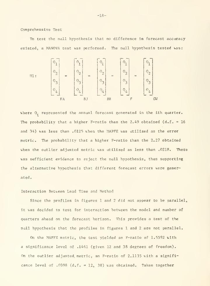
Comprehensive Test

To test the null hypothesis that no difference in forecast accuracy

existed, a MANOVA test was performed. The null hypothesis tested was:

HI:

\ V \ V V°2 °2 °2 °2 ^2

°3 Q3 °3 °3 ^3

°4I

°4 \ ^4 °4

FA BJ BR GW

where 0. represented the annual forecast generated in the ith quarter.

The probability that a higher F-ratio than the 2.49 obtained (d.f. = 16

and 34) was less than .0125 when the MAPFE was utilized as the error

metric. The probability that a higher F-ratio than the 2.27 obtained

when the outlier adjusted metric was utilized as less than .0218. There

was sufficient evidence to reject the null hypothesis, thus supporting

the alternative hypothesis that different forecast errors were gener-

ated.

Interaction Between Lead Time and Method

Since the profiles in figures 1 and 2 did not appear to be parallel,

it was decided to test for interaction between the model and number of

quarters ahead on the forecast horizon. This provides a test of the

null hypothesis that the profiles in figures 1 and 2 are not parallel.

On the MAPFE metric, the test yielded an F-ratio of 1.5592 with

a significance level of .1461 (given 12 and 38 degrees of freedom).

On the outlier adjusted, metric, an F-ratio of 2.1135 with a signifi-

cance level of .0398 (d.f. = 12, 38) was obtained. Taken together

-19-

these tests tend to indicate that there is an interaction between

method and lead time.

Tests Between Specific Models

Since the results of the MANOVA test indicated that a statistically

significant difference existed, more detailed tents were conducted.

In order to determine which of the models differed in performance,

vector comparisons of the equality of the forecast errors were tested

between the financial analysts model and each of the univariate models.

The results of these multivariate tests are contained in Table 5. Since

the lowest probability exceeds 13 percent, these results indicated that

there was insufficient evidence to reject the null hypothesis that no

difference in forecast error accuracy existed between any of the vector

comparisons for either of the error metrics.

TABLE 5

Results of the Multivariate Testof Equality of Mean Vectors

VectorComparison

Error MetricMAPFE OAMAPFE

F-ratio P F-ratio P

FA vs BR . .51 .73 .56 .69

FA vs BJ . .54 .71 .97 .43

FA vs GW 1.73 .16 1.86 .13

FA vs F .50 .73 1.73 .16

-20-

The non-significance of these specific tests indicates that rejec-

tion of HI was largely due to the interaction effect. The net inter-

pretation is that the relative forecasting accuracy of the 5 methods

depends on the quarter in which the forecast is made.

Tests Between Specific Quarters

An additional null hypothesis tested was that no difference in

annual forecast accuracy existed between the quarters in which the

annual forecasts were generated. Since the probability of obtaining

the F-ratio of 3.68 was less than .0184 when MAPFE was utilized and

the probability of obtaining the F-ratio of 22.03 was less than .0001

when OAMAPFE was utilized, there was sufficient evidence to reject

the null hypothesis for both error metrics. Thus, the alternative

hypothesis that forecast accuracy differed from quarter to quarter

was supported.

As evidenced in Figures 1 and 2, the means of the forecast error

metrics decreased as the annual forecasts contained a smaller number

of quarterly forecasts. A test for linear trend between quarters re-

sulted in an F-ratio of 6.83 for the mean absolute percentage error

and an F-ratio of 66.55 for the adjusted error metric. The probability

of obtaining a higher value was less than .012 for the former and .0001

for the latter. The tests between quarters indicated then that not

only did forecast accuracy differ between quarters, but that the

accuracy significantly improved from annual forecast to annual fore-

cast as the year progressed.

-21-

SUMMARY AND CONCLUSIONS

The results of this study must he considered in relation to cer-

tain limitations. First, noncalendar reporting firms, newly formed

firms, and firms that went out of business systematically were excluded

from the sample. The results also were conditioned on the use of

two error metrics. Finally, the purpose considered in this paper was

limited to the ability of the 5 models to predict annual earnings

figures from forecasted quarterly figures.

These results indicated that when the use of univariate time series

models was compared to the financial analysts model, the comparison

favored the financial analysts. When the mean absolute percentage

error metric was utilized, the financial analysts generated a mean

error of .10 when only one quarterly forecast was included in the

annual forecast. This error was 5 percentage points lower than the

best performing univariate model. This difference increased to greater

than 6, 12 and 17 percentage points as the annual forecasts included

two, three and four quarterly forecasts. The standard deviation in

each quarter also was lowest for the financial analysts. In addition,

the financial analysts generated outliers greater than 3.0 that were

lower both in number and degree than the univariate models.

When the error metric was adjusted for these outliers, the mean

errors for the univariate models decreased by at least 18, 14, 9 and

5 percentage points respectively during successive quarters of the

year. The mean error for the financial analysts, however, only de-

creased by 3, 2, 3 andil percentage points respectively. The range

between the best performing and worst performing models decreased

-22-

therefore to a maximum of 4 percentage points. The FA models per-

formed better than the BR, BJ and F models in all four quarters; the

FA model, however, only performed better than the CW model in the first

and fourth quarter.

Therefore the financial analysts tended to out-perform the

statistical models on the adjusted metric with the exception of the

GW model in the first 3 quarters.

Overall multivariate tests (for both error metrics) indicated the

5 methods, viewed simultaneously, are not equal with respect to fore-

cast error. Significant tests and analysis of the profiles indicated

that this overall difference is largely caused by an interaction between

the quarter in which the annual forecast is made and the forecast method

used. In particular the advantage of the FA over the statistical models

tended to decrease as the end of the year approached.

The results further indicated that the premier model suggested by

Brown and Rozeff performed better than an individually identified uni-

variate model in each of the quarters for both of the error metrics.

Thus, there was little justification for selecting the more subjec-

tively and costlier determined individually estimated model. There

also was little empirical support for the premier model considered by

Foster. For both error metrics, this model consistently ranked as the

poorest performing model. Additional evidence therefore was provided

that quarterly earnings are characterized by both a regular and a

seasonal component.

A further consideration is that the smallest mean absolute percen-

tage forecast error generated in each of the four quarters exceeded 34,

-23-

28, 21 and 10 percent respectively as fewer quarterly forecasts were

included in the annual forecast. With the outlier adjusted error metric,

the smallest mean value in each quarter slightly decreased, but still

exceeded 31, 26, 18 and 9 percent respectively. This may indicate that

errors associated with annual forecasts may be so great, especially in

the beginning quarters of the year, that forecasts from the present

sources widely available may have limited usefulness. This question,

however, best can be answered through more comprehensive knowledge of

the use of forecasted earnings by decision makers.

-24-

FOOTNOTES

For a comprehensive treatment of previous research in this area,see Abdel-khalik and Thompson [1977-781.

2Since this process has been the subject of a growing amount of

research, we Kill omit a detailed specification of the process.Interested readers are directed to Rox and Jenkins fl970] or Nelson[1973].

3The F model differs from the model proposed by Foster in that the

drift term is excluded based on evidence provided by Brown and Rozeff[1978] that this term is significant.

AThe selection of an error metric assumes that a certain utility

function is the most appropriate for evaluating alternative forecastingsources. This selection is arbitrary since little is known about theutility function of the users of earnings forecasts. In addition, amore complete analysis would require specification of the loss functionspecific to the investment decision.

The selection of the value of 3.0 as an indication of an outlierwas based on a visual analysis of the frequency distribution of theabsolute percentage forecast error metric. As noted in a subsequentdiscussion, only 54 (1.05%) of the 5000 total forecasts required thisadjustment.

An excellent description of the use of the orthogonal polynomialMANOVA on single factor repeated measure designs Is provided by McCalland Appelbaum [1973], Also see Finn [1974] and Morrison [1967] a

rigorous development of the multivariate general linear model.

In particular the error correlation matrix from the orthogonalpolynomial design must be of type H as discussed by Huynh and Field[1970], With respect to the present study, tests revealed this assump-tion to be strongly violated.

-25-

APPENDIX

Listing of Sample Firms

1. Abbott Laboratories2. Allied Cbemical3. American Cyanamid4. American Seating5. American Smelting6. Bethlehem Steel7. Borg-Warner8. Bucyrus-Erie9. Clark Equipment

10. Consolidated Natural Gas11. Cooper Industries12. Cutler - Hammer13. Dr. Pepper14. Dupont15. Eastman Kodak16. Eaton Corporation17. Federal - Mogul18. Freeport Minerals Co.

19. General Electric20. Gulf Oil21. Hercules, Inc.

22. Hershey Foods23. Ingersoll - Rand24. International Business Machines25. International Nickel Co.

26. Lamsas City Southern Industries27. Lehigh - Portland28. Mead Corporation29. Merck and Company30. Mohascp Corp.

31. Moore McCormack32. Nabisco, Inc.

33. National Gypsum34. National Steel35. Northwest Airlines36. Peoples Drug Stores37. Pepsico, Inc.

38. Rohm and Haas39. Safeway Stores40. Scott Paper41. Square D

42. Stewart - Warner43. Texaco, Inc.

44. Trans World Airlines45. Union Catbide46. Union Oil (Cal.)47. U.S. Tobacco48. Westinghouse Electric49. Weyerhaeuser, Inc.

50. Zenith Radio

-26-

REFERENCES

Abdel-khalik, A. R. and Thompson, R. B. , "Research on Earnings Fore-casts: The State of the Art," The Accounting Journal (Winter1977-78), pp. 180-209.

Anderson, T. W. , Introduction to Multivariate Statistical Analysis .

New York: Wiley Press, 1958, p. 2.

Bock, R. Darrell, Multivariate Statistical Methods in Behavioral Re-search . McGraw-Hill, 1975.

Box, G. E. P., and Jenkins, G. M. , Time Series Analysis: Forecastingand Control . Holden-Day, 1970.

Brov.n, L. D. and Rozeff, M. S., "The Superiority of Analyst Forecastsas Measures of Expectations: Evidence from Earnings," Journal of

Finance (March 1978), pp. 1-16.

, "Univariate Time Series Models of Ouarterly Earnings Per

Share: A Proposed Premier Model," Forthcoming: Journal of

Accounting Research (Spring 1979).

Cragg, J. G., and Malkiel, B. G. , "The Consensus and Accuracy of Some

Predictions of the Growth of Corporate Earnings," Journal of Finance

(March 1968), pp. 67-84.

Elton, E. J., and Gruber, M. J., "Earnings Estimates and the Accuracyof Expectational Data," Management Science (April 1972), pp.409-424.

Financial Accounting Standards Board, Statement of Financial AccountingStandards No. 1; Objectives of Financial Reporting and Elements of

Financial Statements of Business Enterprises . FASB, 1977.

, FASB Discussion Memorandum: Interim Financial Accounting and

Reporting . FASB, 1978.

Finn, J. D. , A General Model for Multivariate Analysis . Holt, Rinehart,and Winston, 1974.

Foster, G. , "Ouarterly Accounting Data: Time Series Properties and

Predictive-Ability Results," Accounting Review (January 1977),

pp. 1-21.

Griffin, P. A., "The Time Series Behavior of Quarterly Earnings: Pre-

liminary Evidence," Journal of Accounting Research (Spring 1977),

pp. 71-83.

Harris, R. J., A Primer' of Multivariate Statistics . New York: AcademicPress, 1975.

-27-

Huynh, Huynh and Leonard S. Feld, "Conditions Under Which Mean SquareRatios in Repeated Measurements Designs Have Exact F-Distributions,"Journal of the American Statistical Association (December 1970),pp. 1582-1589.

Ito, K. , "On the Effect of Heteroscedacticity and Nonnormality Upon SomeMultivariate Test Procedures," in Multivariate Analysis II , ed.Krishnaiah, P. R. New York: Academic Press, 1969.

Lorek, K. S. , "Predicting Annual Net Earnings with Ouarterly EarningsTime Series Models," Forthcoming: Journal of Accounting Research(Spring 1979).

McCall, Robert B. , and Mark I. Appelbaum, "Bias in the Analysis ofRepeated Measures Designs: Some Alternative Approaches," ChildDevelopment (December 1973), pp. 401-415.

McKeovcn, J. C. and Lorek, K. S. , "A Comparative Analysis of Predict-ability of Adaptive Forecasting, Reestimation and ReidentificationUsing Box-Jenkins Time Series Analysis," Decision Sciences (October1978).

Morrison, D. F. , Multivariate Statistical Methods . McGraw-Hill, 1967.

Nelson, C. R. , Applied Time Series Analysis for Managerial Forecasting .

Holden-Day, Inc., 1973.

Watts, R. , "The Time Series Behavior of Quarterly Earnings," UnpublishedPaper, Department of Commerce, University of Newcastle (April 1975).

D/31

' WJH. I' W IIIHL