I

9th Int'! Conference on Inspection, Appraisal, Repairs & Maintenance of Structures: 20 - 21 ober 2005, FtJzhou, China

A NEW INTEGRATION ALGORITHM FOR THE FINITE ELEMENT ANALYSIS OF ELASTO-PLASTIC PROBLEMS

K. Z. Ding*, The Australian National University, Canberra, Australia Q.-H. Qin, The Australian National University, Canberra, Australia

M. Cardew-Hall, The Australian National University, Canberra, Australia

Abstract

The Finite Element analysis of the elastic-plastic behavior is of fundamental importance in automobile industry. To predict accurately the final geometry of the structure and the distribution of strain and stress, accurate integration of the constitutive laws over the strain path is essential. Our objective in this paper is to develop an effective and accurate stress integration scheme for the analysis of three-dimensional sheet metal forming problems. The proposed algorithm is based on the explicit "substepping" schemes incorporating with the stress correction scheme. The proposed algorithms have been implemented into ABAQUS/Explicit via User Material Subroutine (VUMAT) interface platform. The results indicate that the explicit schemes with local truncation error control, together with a subsequent check of the consistency conditions, lead to the accurate results for integrating large elastic­plastic problems.

Keywords: Finite element analysis, Stress integration, Nonlinear elastic-plastic problems.

1 Introduction

.,' Finite element analysis of elastic-plastic behaviour is a sl1l5ject of great importance in various

industrial engineering, as elastic-plastic modelling can help us make a more complete use of strength resources of solids and leads to an efficient method for calculating details of machines and structures as regards to their load-bearing capacity. It is well-known that the accuracy with which the constitutive models are integrated has a direct impact on the overall accuracy of the analysis.

Most commonly used stress update schemes for integration of elastic-plastic constitutive laws fall within the categories of forward (explicit) and backward (implicit) algorithms. During the past decades, implicit algorithms have drawn growing attentions for their excellent convergent performance in nonlinear analysis. Implicit methods are attractive because the resulting stress states automatically satisfy the yield criterion to a specified tolerance. Furthermore, with implicit algorithm the determination of the initial yielding state, i.e. the intersection with the yield surface, becomes unnecessary if the stress point changes from an elastic state to a plastiC state. However, if the complicated constitutive models, which involve non-associated flow rule, complex yield criteria and hardening laws, are used, application of the implicit algorithms is quite often cumbersome and the convergence is not always guaranteed.

Compared with impliCit algorithms, the explicit algorithm has the advantage of being more straightforward to implement. The best-known explicit method for integrating elastic-plastic stress-strain relations is forward Euler scheme. However, for the applications with relative large load increments, the computed stresses may not satisfy the yield criterion after integration process. Therefore, a correction of stresses has been used frequently to prevent the computed stresses from deviating too far from the yield surface.

A number of integration algorithms therefore were developed with the aim to control the error in the integration process. Among them, two explicit schemes with adaptive substepping developed by Sloan([1, 2]), the modified Euler scheme and the Runge-Kutta-England scheme, have drawn many authors' attentions. However, these integration schemes have not been tested for analyzing large-strain .. ',.. t e:llhe-+o""" .... i ... - __ L-.. __ _ _ • - • ,, ­

However, they are superior to the implicit schemes when some form of the stress correction is applied at the end of step.

In this paper, the performance of the implicit and explicit schemes with stress correction is investigated by conducting an elastic-plastic analysis of a typical three dimensional sheet metal forming process. An outline of the paper is as follows. Section 2 presents a fundamental elastic-plastic stress-strain formulation used in the elastic-plastic finite element computations. In Section 3, the proposed integration scheme, the modified Euler scheme, incorporating with stress correction approaches, are described in details. Numerical experiments are reported in Section 4 and concluding remarks are offered in Section 5.

2 Fundamental elastic-plastic formulation

In this study, the elastic and isotropic hardening plastic model appeared in [3] is used for elastic-plastic analysis. Starting from the assumption that there is an additive relationship between strain increment In the present study, we present an elastic and isotropic hardening plastic model. Starting from the assumption that there is an additive relationship between strain increment:

(1)

where !::J.c: is the total strain increment, !::J.C: e is the increment of elastic strain, and !::J.C:p is the increments of plastic strain. The elastic strain rate increment is given by Hooke's law

(2)

and the increments of plastic strain ca[l-ee determined from the associated flow rule, that is:

(3)

where A is a proportionality constant termed the plastic multiplier, F(a, K,) is the yield function and lI:(tp ) is a strain hardening function_ The Von Mises yield criterion is adopted in the present study, that is:

(4)

with ay is determined from: a y = ay

O + K !::J.tp n (5)

in which a~ denotes the initial yield stress and t; represents the effective plastic strain. K and n are the hardening coefficient and hardening exponent respectively. By differentiating the yield function F (a, 1\;) = 0 and using the Eq.(1 )-(3), we obtain the complete elastic-plastic incremental stress-strain relation to be

(6)

with Dep written as

D - D _ De : a : aT : De (7) ep - e H + aT : D e : a

in which

T . 8F [8F 8F 8F 8F 8F 8F]a =-= ----.----- (8)8a 8az ' 8ay ' 8az ' 8Tzy ' 8Tyz ' 8Tzz )

1 8FH = ---!::J.K, (9)

!::J.A 8K,

It is well-known that the method for integrating elastic-plastic stress-strain relations is to divide the integra­tion process into several substeps and compute the stress-strain response over each substep. Its accuracy increase, of course, with the number of substeps. But the computation for each substep is time-consuming, since the flow vector and eJastoplastic matrix have to be calculated at each stage_ Clearly, a balance must be solved _ Traditionally, the number of substeps is determined from an empirical rule and each substep is assumed to be of the same size. Such integration will generally result in the stress change departing from the y~ eld surface, aAQ. a proportional scaling of stresses have been frequently used to (estore them to the yield sur-

I face. Although this method has been used widely in the finite element codes, it have following disadvantages:

1. If the correction-step is applied after each substep, the computational time will increase drastically. How­ever if' . . ·fic. n Iv ;:)ffAr.t thp l'Ir:r:llr::lr.vrJ11

2. Since the number of substeps is usually determined by an empirical rule which is formulated by trial and error, the inappropriate choice of the number of the substeps usually leads to lose of either accuracy or efficiency.

In the following section, a substepping scheme is used, which can be used to integrate the elastic-plastic stress-strain relation with a aim to control the error by adjusting the size of each substep automatically. There­fore it can avoid to increase the number of substeps blindly just for a moderate accuracy.

3 Integration of the stress-strain relations

The following procedure is commonly adopted for elasto-plastic analysis. Within a particular load incre­ment T, the strain increments t:.€r can be determined via the displacement increments. Once the strain have been determined, the stress increments may be calculated using Hooke's law under the assumption of elastic behaviour:

and a trial stress state is obtained through

(10)

(11 )

The trial stress a[rial is then tested in F(a[rial' /l:r-l). If F(a~rial' /l:r- J) ::; 0, then the elasticity assumption is taken to be valid, and a[rial is considered as the new stress state. If F(a;rial' /l:r-l) > 0, the plastic yielding occurs. In this case, the final stress state is needed to determine by integrating the the stress-strain relations

, over the strain path. The integration of stress-strain relations requires the solution of the initial value problem like

da II = Dep t:.E. , T E [0 , 1] (12)

in which alT=o defines the stress state which already satisfy the yield criterion, and alT=l defines the stress at an end of load increment or iteration.

Integrating the constitutive relations to obtain the unknown increment of the stresses is a key step in non­linear elastic-plastic finite element analysis. The methods commonly used at the present are usually classified as explicit or implicit. In an explicit integration scheme, the yield surface. plastic gradients and hardening parameter are all evaluated based on known stress states of last substep. In a fully implicit method, all the internal variables are evaluated at unknown stress states of the current substep, resulting a system of non­linear equations must be solved iteratively. Given that the introduction of commonly used implicit radial return scheme and explicit forward Euler scheme can be found in many reference, such as 8elytschko[6] and Chen[7] Only the substepping scheme is introduced in details.

3.1 Intersection with the yield surface

As mentioned previously, if F(a(r-l) , /I:(r- l») < 0 and F(atrial, /I:(r-l») > o. the plastic yielding occurs during­this increment and the strain increment is partly in an elastic path and partly in a plastic path. Assume that the stress state changes from last elastic state ar

-J to an elastic-plastic state. In order to determine the portion of

the stress which cause purely plastic yielding, we need to find a scalar 0: such that

where

:

to ensure that the stress state at F(a r , /I:(r - l») = 0 lies on the yield surface. A variety of schemes are available for determining scalar 0: . A simple linear interpolation method used in [3] gives:

F(a(r-l» ) 0: = - ---.,---''---.,..:.-,.---.,,,,, (13)

F(atriad - F(a(r-l»)

Sloan[1] used a Newton-Raphson iteration to compute 0:. In this paper. an iterative scheme is used with the aim to maintain sufficient accuracy for the plasticity integration. The intersection point. i.e. 0: may be obtained by iteratively solving

IT,~ = '- , 4

(15)

in which 1\ -F(ak,lI:) U O' Ic + 1 = T 1\ (16)

a le ua rwith the starting point at a o = a -

1 and use the value in Eq.(13) for 0'1. After determining the initial plastic yielding, we must reduce the excess stress onto the yield surface to maintain the consistency condition.

3.2 Correction of the yield surface drift

If the explicit integration schemes are used for updating the stress, the stress state at the end of the incre­ment may not fulfill the yield criterion. The error will essentially depend on the size of the strain increment and number of subdivisions, but as the error is cumulative it is important to ensure that the stresses are corrected back to the yield surface during each increment. Among the five methods of projecting back inl [5], the method called "projecting back along the plastic flow direction" has been proved to be the best one and will be used in this project.

Assume that the initial stress state A locates on the yield surface, i.e. F(aA , II:A ) = 0 and the new stress state after integration B drifts away from the updated yield surface F(aB , II:B) = O. The stress state C repre­sents the stress state after correction . Due to the nature of the plastic flow direction normal to the yield surface for von Mises plasticity, we have:

8F ac = aB - /3- (17)

8a where /3 ,is a scalar quantity. Since the hardening parameter remains unchanged, we have the updated yield condition as:

F(ac,lI:c) = F ((aB -/3~:) , II:B) = 0 (18)

The updated scalar /3 can be obtained by a Taylor series expansion:

F(aB,II:B)/3 = (19)

(~~) (~~) T

F(aB,II:B) (20)

a : aT

It is generally suggested to check that the yield criterion is fulfilled to some tight tolerance after correction . If this is not the case, an iterative procedure is then necessary with the starting point of a o = ab and 11:0 = II:b .

3.3 Modified Euler method

The modified Euler scheme with active error control was introduced in Sloan[1] and Jakosen[8] with the aims to reduce yield surface drift and computational costs of the forward Euler scheme. Instead of using a constant substep size, this explicit scheme uses the difference between the solutions obtained with two embedded Euler algorithms of different order of accuracy to extrapolate the substep size which can achieve a prescribed accuracy of the solution.

By defining a dimensionless time T such that T E (0,1) , the strain increment for a substep k is given

(21)

The first estimate of t~e updated stress and the hardening parameter at the end of the substep is given by:

a = ao + 6a1 (22)

II: = 11:0 + 611:1 (23)

where

6a1 Dep (ao , lI:o )6c(k)

611:1 = 6'\ (ao, 11:0, oc(Ie))h

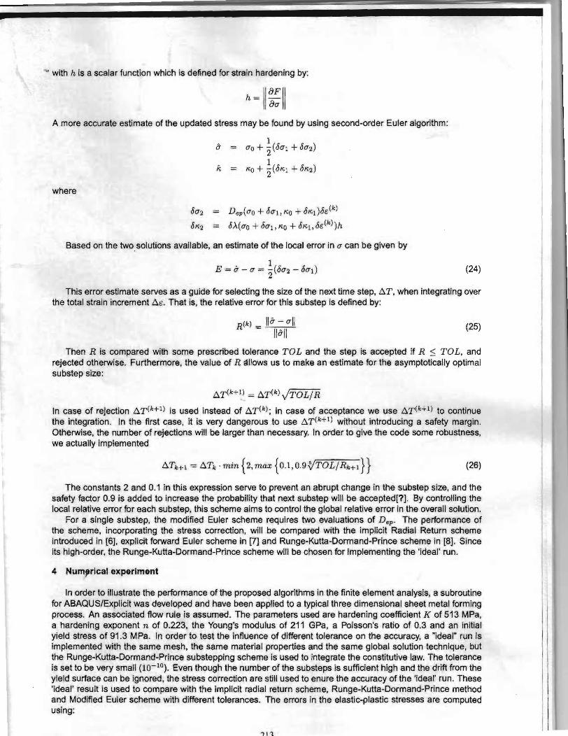
with h is a scalar function which is defined for strain hardening by:

h=II:11 A more accurate estimate of the updated stress may be found by using second-order Euler algorithm:

1 CT = 0"0 + 2" (00"1 + 00"2)

1 k /1:0 + 2(OKI + OK2)

where

00'2 Dep(O"O + 00'1, KO + OKdoE(k)

OK2 0'\( 0"0 + 00'1, KO + OKl, &(k))h

Based on the twosolutions available, an estimate of the local error in a can be given by

E = CT - 0" = ~(oa2 - oO"I) (24)2

This error estimate serves as a guide for selecting the size of the next time step, b.T, when integrating over the total strain increment b.E. That is, the relative error for this substep is defined by:

(25)

Then R is compared with some prescribed tolerance TaL and the step is accepted if R ~ TaL, and rejected otherwise. Furthermore, the value of R <tllows us to make an estimate for the asymptotically optimal substep size:

b.T(k+l) = b.T(k) y!TOL/R

In case of rejection b.T(k+l) is used instead of b.T(k); in case of acceptance we use b.T(k+l) to continue the integration. In the first case, it is very dangerous to use b.T(k+l) without introducing a safety margin. Otherwise, the number of rejections will be larger than necessary. In order to give the code some robustness, we actually implemented

b.Tk+l = b.Tk . min {2, max {0.1, 0.9 {jTOL/Rk+l} } (26)

The constants 2 and 0.1 in this expression serve to prevent an abrupt change in the substep size, and the safety factor 0.9 is added to increase the probability that next substep will be accepted[?]. By controlling the local relative error for each substep, this scheme aims to control the global relative error in the overall solution.

For a single substep, the modified Euler scheme requires two evaluations of Dep. The performance of the scheme, incorporating the stress correction, will be compared with the implicit Radial Return scheme introduced in {6], explicit forward Euler scheme in [7] and Runge-Kutta-Dormand-Prince scheme in f8]. Since its high-order, the Runge-Kutta-Dormand-Prince scheme will be chosen for implementing the 'ideal' run.

4 Num~rical experiment

In order to illustrate the performance of the proposed algorithms in the finite element analysis, a subroutine for ABAQUS/Explicit was developed and have been applied to a typical three dimensional sheet metal forming process. An associated flow rule is assumed. The parameters used are hardening coefficient K of 513 MPa, a hardening exponent n of 0.223, the Young's modulus of 211 GPa, a Poisson's ratio of 0.3 and an initial yield stress of 91.3 MPa. In order to test the influence of different tolerance on the accuracy, a "ideal" run is implemented with the same mesh, the same material properties and the same global solution technique, but the Runge-Kutta-Dormand-Prince substepping scheme is used to integrate the constitutive law. The tolerance is set to be very small (10- 10) . Even though the number of the substeps is sufficient high and the drift from the yield surface can be ignored, the stress correction are still used to enure the accuracy of the 'ideal' run. These 'ideal' result is used to compare with the implicit radial return scheme, Runge-Kutta-Dormand-Prince method and Modified Euler scheme with different tolerances. The errors in the elastic-plastic stresses are computed using:

,}1

: :::~:] . , ~ ,,~\))r;" " .$ ..v" ....

4 OOE'OOB ~ .~ • : : : : . : . : - :.: - ::: .... ..... . . ...--­.....f .: ~ .: .. .~___

:::::::('t,:' : ~~1~' ."....J

100"008 ModIfied Euler(TOL:lo',10~ , RKDP(TOL=10 ', IO ', IO',lO" ,1·0·)

5.00E.ooaj .. ... .::,.~ . ... ..-.....-.. .,.. 4.00E·OQ8 ..".:.-- -- ....... '" .,....

• 3.00e.006 ;.•.. '

- . • - - Ideal c~ 13l 2.00e..ooa Backward & UJ

FEC. MEC~ .,.10" ) 1.00E+OOB f

RKDPC( n " · 10·').MEC(10'.I O". IO"j

~ ooo a -.-- I , , iii I a.ooe. +'~--"I ~-"-~--r,.......-,-,---.,-~r-,­

0.0 0.1 0.2 0.3 0.4 0. 5 0.8 0.7 0.0 0 .1 0.2 0.3 0 " O.S 0.6

Effective plasi je st r ai n errectlc plasflcSin

Figure 1: Effective plastic strain - Effective stress curves. (a) - Explicit schemes without the stress correction. (b) - Explicit schemes with the stress correction.

where N is the total number of the integration pOints. For each explicit scheme, two different models are studied, i.e. with and without stress correction respectively.

Note that in all the following figures and tables, "* * **" denotes the aborted solution due to the serious distortion caused by the incorrect integration. RR, FE, ME and RKDP denote the redial return scheme, forward Euler scheme, Modified Euler scheme and Runge-Kutta-Dormand-Prince scheme, respectively. FEC, MEC and RKDPC mean that stress correction is applied for these schemes.

4.1 Accuracy

In Fig. (1), we present strain-stress curve for the deep cup drawing process. With reference to Fig. (1), we can find that, for the cases of large plastic strain problem, the results computed by the explicit schemes without stress correction are almost same no matter how tight we set the error tolerance. However, the results are completely different if the stress correction is employed. In fact, without stress correction, all the three explicit schemes can not give the satisfactory accuracy for the case which involves strain hardening when the tolerance is 10- 5 and smaller. We can see from Fig. (1) that the forward Euler scheme gives the worst result without the stress correction, and the radial return scheme gives relatively accurate result. It is worth noting that even the Runge-Kutta-Dormand-Prince is insensitive to the error tolerance for the deep drawing process, although the accuracy is improved as the error tolerance gets tighter. This again proves that, because the approximation nature of the finite element method, yield surface drift may occur with the stresses moving away from the yield surface. This deviation is practically independent of the integration scheme adopted. When the model involves strain (work) hardening where the yield surface is moving with loading increment, the drift is more significant. Since such discrepancies are usually cumulative, it is important to ensure the the stresses are corrected back to the current yield surface at each step of the integration. Since we apply the stress correction at the end of each time increment, it does not affect the accuracy significantly. However, it can make the computed stress to fulfill the consiste~y condition at the end of load increment and avoid error accumulation and therefore instabilities in the following time increments. It is also interesting to see that the the rad ial return scheme gives the relatively accurate result at the last several increments, although its strain-stress curve still drifts away from the ideal one during some of the time increments.

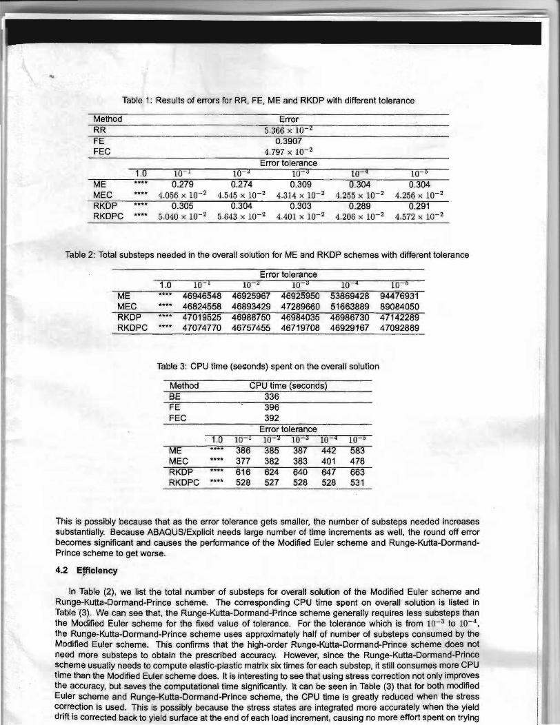
The errors in the computed stresses from different algorithms with different tolerance are listed in Table (1) . With reference to Table (1), it can be seen that, the Backward Euler scheme gives good result which is adequate for the engineering computation, compared with the explicit schemes. For the cases in which stress correction is applied for the explicit schemes, all the explicit schemes give the better results than the Backward Euler scheme. In (1]', the measure of error which is approximately equal to tolerance was obtained. However, as mentioned previously, the results obtained from Modified Euler scheme aDd Runge-Kutta-Dormand-Prince scheme are not improved as the error tolerance becomes tighter. This again indicates that the stress correction applied at the end of each load increment does not ,il1)prove the performance significantly. On the opposite, the smallest error tolerance, i.e. 10- 5 , always makes the accuracy worse. The similar result has been shown in t8].

...

Table 1: Results of errors for RR, FE, ME and RKDP with different tolerance

Method Error RR 5.366 x 10 2

FE 0.3907 FEC 4.797 x 10-2

Error tolerance 1.0 10 10 2 10 :J 10 ~ 10 "

ME MEC

****_.*. 0.279 4.056 x 10-2

0.274 4.545 X 10-2

0.309 4.314 X 10- 2

0.304 4.255 X 10-2

0.304 4.256 X 10-2

RKDP ***. 0.305 0.304 0.303 0.289 0.291 RKDPC •••• 5.040 x 10-2 5.643 X 10-2 4.401 X 10-2 4.206 X 10-2 4.572 X 10-2

Table 2: Total substeps needed in the overall solution for ME and RKDP schemes with different tolerance

Error tolerance

ME 1.0••*.

10 1

46946548 10 2

46925967 10 3

46925950

10 ~ .

53869428 10 5

94476931 MEC *••• 46824558 46893429 47289660 51663889 89084050 RKDP *••• 47019525 46988750 46984035 46986730 47142289 RKDPC ••*. 47074770 46757455 46719708 46929167 47092889

Table 3: CPU time (seconds) spent on the overall solution

Method CPU time (seconds) BE 336 FE 396 FEC 392

Error tolerance ~ . 1.0 10 10 2 10 :J 10 10 "

.***ME 386 385 387 442 583 MEC **** 377 382 383 401 478 RKDP .'*.* 616 624 640 647 663 IRKDPC .*.* 528 527 528 528 531

This is possibly because that as the error tolerance gets smaller, the number of substeps needed increases substantially. Because ABAQUS/Explicit needs large number of time increments as well, the round off error becomes significant and causes the performance of the Modified Euler scheme and Runge-Kutta-Dormand­Prince scheme to get worse.

4.2 !EffiCiency

In Table (2), we list the total number of substeps for overall solution of the Modified Euler scheme and Runge-Kutta-Dormand-Prince scheme. The corresponding CPU time spent on overall solution is listed in Table (3). We can see that, the Runge-Kutta-Dormand-Prince scheme generally requires less substeps than the Modified Euler scheme for the fixed value of tolerance. For the tolerance which is from 10-3 to 10-4 ,

the Runge-Kutta-Dormand-Prince scheme uses approximately half of number of substeps consumed by the MOdified Euler scheme. This confirms that the high-order Runge-Kutta-Dormand-Prince scheme does not need more substeps to obtain the prescribed accuracy. However, since the Runge-Kutta-Dormand-Prince scheme usually needs to compute elastic-plastic matrix six times for each substep, it still consumes more CPU time than the Modified Euler scheme does. It is interesting to see that using stress correction not only improves the accuracy, but saves the computational time significantly. It can be seen in Table (3) that for both modified Euler scheme and Runge-Kutta-Dormand-Prince scheme, the CPU time is greatly reduced when the stress correction is used. This is possibly because the stress states are integrated more accurately when the yield drift is corrected back to yield surface at the end of each load increment, causing no more effort spent on trying

to correct the accumulative errors in the following increments. Note that, unlike in [1], the Runge-Kutta-England scheme has a significant advantage over the modified Euler scheme, in the present study, the performance of the Runge-Kutta-Oormand-Prince scheme is almost same as it of the Modified Euler scheme. On the opposite, when the stress correction is employed, the Modified Euler scheme is better than the Runge-Kutta-Dormand­Prince scheme. This is possibly because that, since the Modified Euler scheme uses much more substeps than the Hunge-Kutta scheme, the deviation from the yield surface is relatively smaller. In spite of this, both schemes can give satisfactory results for the engineering problem if the stress correction is used.

5 Conclusion remarks

In this paper, we present two substepping schemes, modified Euler and Runge-Kutta-Oormand-Prince schemes with local error control, enhanced by the stress correction procedure, for analyzing the elastic-plastic problems. Their performances have been compared with the commonly used implicit and explicit integration schemes, including Radial return algorithm, forward Euler with subincrementation. The numerical example indicated that, for the large strain three-dimensional problem of which the strain hardening is considered, the accuracy can not be improved significantly as the tolerance decreases. Some forms of stress correction should thus be employed in order to ensure that the computed stresses remain on the yield surface at any time and maintain adequate accuracy of the overall solution. In summary, the experience suggests that

1. For large strain three dimensional problem, neither of the explicit schemes with error control can give accurate result without the application of the stress correction .

2. High order Runge-Kutta-Oormand-Prince is not superior to the second order modified Euler scheme in this case.

3. It has been shown that the combination of the modified Euler scheme with the stress correction offers the accurate and efficient integration even for a smaller error tolerance.

References

[1] Sloan Sw. Substepping Schemes for the Numerical Integration of Elastoplastic Stress-strain Relations. tnt. J. Numer. Methods Eng. 1987;24:893-911.

[2] Sloan SW, Booker JR. ,Integration of Tresca and Mohr-Coulomb Constitutive Relations in Plane Strain Elastoplasticity. Int. J. Numer. Methods Eng. 1992;33:163-196.

[3] Owen DRJ, Hinton E. Finite Elements in Plasticity: Theory and Practice, Pineridge Press, Swansea, U.K. 1980.

[4] Wissmann JW, Hauck C. Efficient Elastic-Plastic Finite Element Analysis with Higher Order Stress-Point Algorithms. Comput. Structures 1983; 17( 1 ):89-95.

[5] Potts OM, Gens A. A Critical Assessment of Methods of Correcting for Drift from the yield surface in Elasto-plastic Finite Element Analysis. Int. J. Numer. Methods Eng. 1985;9:159-149.

[6] Belytschko T, Liu WK, Moran B. Nonlinear Finite Elements for Continua and Structures. John Wiley and Sons Ltd 1994.

[7] Chen WF. Constitutive Equations for Engineering Materials. Elseview Science 2000;Volume 2: Plasticity and Modeling.

[8J Jakobsen KP, Lade pv. Implementation algorithm for a single hardening constitutive model for frictional materials. Int. J. Nvmer. Anal. Meth. Geomech 2002;26:661-681.

[9J Luccioni LX, Pestana JM, Taylor RL. Finite element implementation of non-linear elastoplastic constitutive laws using local and global explicit algorithms with automatic error control. Int. J. Numer. Methods Engng. 2001 ;50: 1191-1212.

[101 Crisfield MA. Non-linear Finite Element Analysis of Solids and Structures. John Wiley and Sons Ltd 1997;Vol. 2 Advanced Topics.

[11] Zienkiewicz OC, Taylor Rl. The Finite Element Method, McGraw-Hili Book Company 1991 . -