a new recycling-rescaling method for large eddy simulation of turbulent atmospheric ...€¦ ·...
TRANSCRIPT

A New Recycling-Rescaling Method for Large Eddy Simulation of Turbulent Atmospheric Boundary Layer
*Chao Li1), Jinghan Wang2) and Yiqing Xiao3)
1), 2), 3) Shenzhen Graduate School of Harbin Institute of technology, Shenzhen,
Guangdong, China, 1)
ABSTRACT
The recycling-rescaling method has been extended to simulate micro-scale turbulent atmospheric boundary layer (ABL), in which staggered blocks were placed in the developing section same as the physical ABL wind tunnel. However, poor efficiency and limited boundary layer thickness restrict its popularity in computational wind engineering (CWE). To improve the existing method, the heart of our new recycling- rescaling method is to generating a controllable inlet condition based on the feedback of downstream solution. Our new method retains “recycling” but redefines “rescaling”. The rescaling of downstream velocity profile is realized by the feedback active control strategy according to the errors between the observed and objective data. The influences of several key parameters for recycling-rescaling based method are tested to achieve the optimal configurations. The large eddy simulation (LES) results corresponding to two terrain types are also analyzed and compared with the prescribed profiles. The results could prove the feasibility and effectiveness of our new method.
1 INTRODUCTION
As lots of super-high rise and long-span structures shows, the wind-induced
fluctuating response received more and more attention. In CWE area, the study of steady wind characteristics using Reynolds-Averaged Navier-Stokes equation (RANS) has been so developed. But another essential problem is in urgent need of being studied, which is to high-fidelity simulate the characteristics of the turbulent ABL.
In wind engineering, since the fundamental theories and flow characteristics of ABL on earth are similar to turbulent flat plate boundary layer (FPBL), it is appropriate to treat ABL as a planetary-scale and non-smooth FPTBL. Thus the successful simulation results of turbulent FPBL can be good basements for the real ABL cases. At present, one of the efficient simulation methods for spatially developing FPBL is recycling-rescaling method proposed by Lund (1998). This method advocated setting
1), 3)
Professor 2)
Graduate Student

an auxiliary flow field for generating the turbulent inflow data of the main simulation. A recycle plane was placed and a quasi-period boundary condition between inlet and this plane would be formed along the streamwise direction, which can effectively shorten the length of the computation domain. Lund proved the feasibility of this method in generating natural equilibrium turbulent inflow data for the zero-pressure gradient FPBL. However, Kunlun Liu (2006) pointed out the initial condition would affect the length of starting transient, and then proposed a dynamic recycling procedure to remedy this problem. Elain Bohr (2005) also fixed a specified mean velocity profile to help drive the turbulent flow through the transient. Besides, Simens (2007) claimed the non-physical streamwise periodicity phenomenon of Lund’s methodology in numerical simulations. In order to overcome these problems, Jewkes (2008) adopted displacement boundary layer thickness instead of boundary layer thickness as the inlet deterministic variable within the rescaling procedure; also the fluctuating velocity was not rescaled during the simulation. The results showed a great improvement of eliminating the influence of starting transient and periodic phenomenon.
Nozawa and Tamura (2001) advanced Lund’s method to simulate the boundary layer over high-density roughness using a different empirical formula and staggered blocks. Then they (Nozawa and Tamura, 2002) validated the large eddy simulation technique for predicting mean flow characteristics around a low-rise building immersed in the turbulent flow. Even though their study gave good results of mean characteristics, the fluctuating characteristics like wind spectrum and integral length scale were not verified with experimental data. Kataoka (2002) proposed a hypothesis that boundary layer thickness keeps constant in streamwise direction which tremendously simplified the recycling-rescaling method. In his research, roughness elements were used to generate the turbulence and mean velocity showed good consistence with the targets. In addition, the turbulence intensity fixed well to the wind-tunnel experiments and power spectrum density of the velocity fluctuation followed von Karman spectrum well (Kataoka, 2008).
To reproduce fluctuating characteristics of turbulent ABLs above any prescribed surface roughness by Nozawa and Kataoka methods, it is unavoidable to determine the size and density of stagger blocks by trial-and-error in advance, so the efficiency is greatly reduced due to the adjustment process of stagger blocks. In this paper, a new recycling-rescaling method without employing stagger blocks in the computational model is proposed. Our new method retains “recycling” but redefines “rescaling” by adding a dynamic proportional coefficient for fluctuating velocity into the original rescaling procedure. With the aid of feedback control strategy, the coefficient is determined actively by the object and the observed flow turbulence intensity in the downstream.
2 GENERARION METHOD OF INFLOW TURBULENCE
2.1 Lund’s Original Recycling-Rescaling Method
The original recycling-rescaling method was firstly introduced by Lund (1998). As the name implies, this methodology includes two main steps: firstly, set a velocity recycle plane (recycle station) in the downstream of the driven section to recover the velocity every time step. Secondly, rescale the recycled velocities according to the

velocity distribution law of turbulent boundary layer and composite a new velocity field to be the inlet boundary conditions.
Decompose the recycled velocity iu into mean velocity ( iU ) and fluctuating
velocity ( iu ) as shown in Eq. (1). The index i=1, 2, 3 represents the streamwise, lateral
and vertical directions with corresponding coordinates x, y and z. The subscript re and in refer to the recycle station and inlet plane, inner and outer represent the inner layer and outer layer of turbulent FPBL.
iii uUu (1)
)()( inre
inner
in zUγU (2)
reiniini zuu )()( (3)
outer
ini
outer
ini
inner
ini
inner
inirei uUWuUWu )()()()()()(1)( (4)
In above equations, ν
uzz τ
is the wall coordinate and δ
zη is the outer
coordinate. z is the vertical distance against the wall and δ is boundary layer thickness.
The mean coefficient γ is associated with the wall friction velocity τu and
determined by using empirical formula Eq. (5). )(
inre zU and reini zu )( need to be
determined by linear interpolation according to )(
rere zU and rerei zu )( respectively.
8/1
8/1
,
, βθ
θ
u
uγ
in
re
reτ
inτ
(5)
2.2 Nozawa’s Modified Recycling-Rescaling Method
Lund’s original recycling-rescaling method was proved to be reliable in simulating the spatially developing boundary layer over smooth flat plate. In order to broaden the application of this method to simulating the turbulent FPBL over rough surface, Nozawa (2001) chosen an empirical resistance formula of sand-roughened plate Eq. (6) for
and . Eq. (7) gives the expression of parameter r , in which sk is the equivalent
sand roughness of the staggered blocks in computational domain as shown in Fig 1. In addition to these modifications, the other procedures were the same with Lund’s original method.
112
)(1
22
1 r
r
in
fγ
r
x
θ
xCβ -- (6)
sk
xr
log58.187.2
95.3
(7)

recycle
sta
tion
inle
t
Fig 1 Nozawa’s Block Arrangement
2.3 Kataoka’s Simplified Recycling-Rescaling Method In structural wind engineering, the gradient heights of ABL are considered as
constant over the same terrain types. Kataoka (2002) adopted this assumption and simplified the original recycling-rescaling method in simulating the turbulent ABLs. Under this assumption, the mean coefficient equals to 1.0, which leads to the wall
coordinate z and outer coordinate η at any streamwise location are identical.
Therefore, the linear interpolation of velocity from the recycle station to the inlet plane is unnecessary and the rescaling procedure was simplified significantly. The simplified inflow boundary conditions by Kataoka are given by Eq. (8)~Eq. (10). )(zU is the
specified mean velocity profile.
),,()()(),,( tzyuηφzUtzyu rein (8)
),,()(),,( tzyvηφtzyv rein (9)
),,()(),,( tzywηφtzyw rein (10)
However, the actual thickness of boundary layer is increased with its development
and a damping function )(ηφ is used to prevent the fluctuation velocity from
developing in the free stream. Eq. (11) gives the expression for )(ηφ .
)0.8tanh(
3.04.07.0
0.10.8tanh1
2
1
φ(η) (11)
2.4 The New Recycling-Rescaling Method
The motivation of our new method is to simulate any prescribed reasonable fluctuating characteristics of ABLs efficiently, so Kataoka’s assumption is adopted. As shown before, all the fluctuating velocity in previous methods has no proportional calculation during the rescaling process. The reason is that the method is used for generating a zero pressure gradient FPBL in Lund’s study (1998) and FPBL over rough flat plate in Nozawa’s (2001), even in Kataoka’s research (2002) the flow turbulence was generated by roughness elements, thus there is no need to artificially adjust the fluctuating characteristics of the flow field.

Therefore, in order to generate any specified turbulent boundary layer, the recycled fluctuating velocity from downstream will be adjusted artificially prior to be imposed on the inlet plane. The adjustment is realized by constructing a dynamic proportional coefficient ),( tzλ according to the objective and monitored flow turbulence
intensities, which will be implanted in the velocity’s rescaling procedure. Contrary to the mean coefficient γ , ),( tzλ is called the fluctuation coefficient. Eq. (12) ~ (15) present
the approach to calculate this fluctuation coefficient.
),(
)(),(
,
,
tzI
zItzλ
y
reu
obju (12)
y
reu
y
reu tzyItzI ),,(),( ,, (13)
),(
1
),()Δ,,(
),,( 1
2
, zyUN
zyUtizyu
tzyI t
re
N
i
t
rere
reu
(14)
NtzyuzyUN
i
re
t
re
1
),,(),( (15)
In above equations, ydenotes the averaging process in spanwise direction.
),,(, tzyI reu is the instantaneous turbulence intensity and ),( zyU t
re is the time-averaged
mean velocity within time interval tN Δ,0 at recycle station. N is total number of
simulation time steps and tΔ is simulation time step.
Substitute the fluctuation coefficient ),( tzλ into Eq. (8) and the inflow boundary
conditions in streamwise direction is given by Eq. (16). The boundary conditions in y and z directions are the same with Eq. (9) and Eq. (10).
),,(),()()(),,( tzyutzληφzUtzyu rein (16)
2.5 The adjustable key parameters
As mentioned before, the turbulent ABL has similar fundamental theories with spatially developing flat-plate boundary layers, so we will first simulate the micro-scale turbulent boundary to determine the optimal numerical simulation parameters. Different from the strict spatially developing boundary layers, we focus on the flow characteristics at specified plane of computational domain. After lots of test and calculations, we found that initial condition, the way of velocity re-introduced and the position of recycle station will affect the efficiency and accuracy of the numerical simulations.
The initial condition mainly refers to the fluctuating velocity field. We will choose two typical initial fluctuations: one-direction and three-direction random fluctuations used by Lund and Jewkes respectively. They are showed in Table 1.
The second parameter is the way of velocity re-introduced. This represents the manner that scaled velocities be introduced as the inlet boundary conditions. Lund adopted the direct translation way in his simulation, but Spalart (2006) noticed there will exit spurious periodicity when use Lund’s methodology. So they posed a spanwise shift

way to eliminate this kind of phenomenon. Jewkes (2008) advocated another simpler way on this basis called mirror way. The principle of this manner is showed in Eq.(17).
Table 1 Different initial fluctuation
Initializing fluctuation
Fluctuation type
u
v
w
IF1 One-direction )(8.0 zU 0 0
IF2 One-direction GradU1.0 0 0
IF3 Three-direction )(8.0 zU 0.6 0.5
IF4 Three-direction )(9.0 zU 0.7 0.6
Ugrad is the free stream velocity in turbulent FPBL and gradient velocity in turbulent ABL
inyinmi
inyinmi
inyinmi
tzyLwtzyw
tzyLvtzyv
tzyLutzyu
,),(),,(
,),(),,(
,),(),,(
,
,
,
(17)
The third parameter is the position of recycle station. The distance between inlet
and recycle station also associates with the spurious periodicity of flow field. Otherwise, the recycle station can’t be too far from the inlet, otherwise it will be meaningless to use the recycling-rescaling based methods. For comparison, we choose two distances between inlets and recycle plane, i.e. 0.4Lx and 0.8 Lx.
3 NUMERICAL METHOD
CFD solver, FLUENT is employed to produce the turbulent FPBL. LES and
dynamic Smagorinsky-Lilly subgrid-scale model are chosen for all cases. In simulations of smooth FPBL, the inlet boundary condition is user defined function
(UDF) programs of Eq.(4). In LES of rough turbulent ABLs, the inlet boundary condition is UDF programs of Eq. (9), (10) and (16). Except for the inlet boundary conditions, other boundaries are the same for all cases.
Different from the original boundary conditions, we use specified-shear wall (zero shear stress) instead of the zero-vorticity condition at the top surface. At the exit plane, outflow is adopted rather than convection boundary condition. Since we focus on the flow characteristics at specified plane and the effects of top boundary condition can be eliminated by increasing the computational domain heights, the replacement will have little influence on our concerns. The bottom boundary is no-slip wall.
4 RESULTS AND DISCUSSIONS

4.1 LES of smooth flat-plate boundary layer with Re=16000 In this section, we will present the LES results of smooth FPBL on the basis of
Lund’s original recycling-rescaling method. The purpose is to determine the optimal key parameters mentioned in section 2.5.
Since the displacement boundary layer thickness *δ is more controllable, we use this quantity as the control thickness of the inlet for all cases. As shown in Fig 2,
the size of the computational domain is: zyx LLL = 64 *δ 4 *πδ 24 *δ , the recycle
station is placed at 25.6 *δ and 51.2 *δ . The simulation results at middle plane are extracted and processed for comparison. The boundary layer thickness at inlet is
determined according to
ν
δU gradRe 16000.
Two sets of grid divisions are used to verify the grids independency. The first
grids arrangement G1: zyx NNN =100 64 45, and a much finer mesh is G2:
zyx NNN =1509668. The grids are uniformly distributed in x and y directions, and
growing exponentially in z direction with growth factor 1.171 and 1.101 respectively.
The first mesh height against wall satisfies 2.1Δ
wallz .
Fig 2 Computation Model for parameter’s determination The simulation time step is 0.04s for G1 grids and 0.01s for G2 grids. Total
simulation time is 1200s and the time for data statistics is the last 600s. All configurations of 8 cases are listed in Table 2.
In order to verify the accuracy of our simulations, we compare the LES results with Spalart’s (1988) direct numerical simulation results (DNS). After comparing the numerical results of all cases, we found that case DH4 has the shortest time before the simulation getting stable, also generates the realizable fluctuation characteristics and the influence of exit boundary condition is the smallest. The results of DH4 are showed in Fig 3, Fig 5 and Fig 6.

For testing the grid independence, we set FG case. And the simulation results are showed in Fig 4, Fig 7 and Fig 8.
Table 2 Simulation cases to determine the optimal configurations of key parameters
Case Grid type Initial fluctuation Velocity re-
introduced way Distance between inlet
and recycle plane
DH1 G1 IF3 translation 0.4 Lx DH2 G1 IF3 mirror 0.4 Lx DH3 G1 IF3 translation 0.8 Lx DH4 G1 IF3 mirror 0.8 Lx IN1 G1 IF4 mirror 0.4 Lx IN2 G1 IF1 mirror 0.4 Lx IN3 G1 IF2 mirror 0.4 Lx FG G2 IF3 mirror 0.8 Lx
According to the DNS results and in the current Reynolds number, the friction
velocity should be about 0.046, however, in our simulation, the statistical friction velocity is all about 0.036. This underestimation is related to the replaced boundary conditions mentioned in section 3. For verifying the influence of key parameters, we used 0.046 to nondimensionalize the mean and fluctuating components of our results.
Fig 3 Mean velocity of DH4 Fig 4 Mean velocity of FG Fig 3 and Fig 4 show the mean velocity profile at middle plane of DH4 and FG
cases. It’s apparent that the LES result of DH4 is smaller than the DNS results in viscous sublayer region but fit well in logarithmic region. The deviation is greatly reduced in FG case, which can implies that this phenomenon is partly associated with
100
101
102
103
0
5
10
15
20
25
z+
U+
LES
DNS
100
101
102
103
0
5
10
15
20
25
z+
U+
LES
DNS
the grid resolution and finite-difference method, the same phenomenon occurred in Lund’s study (1998).
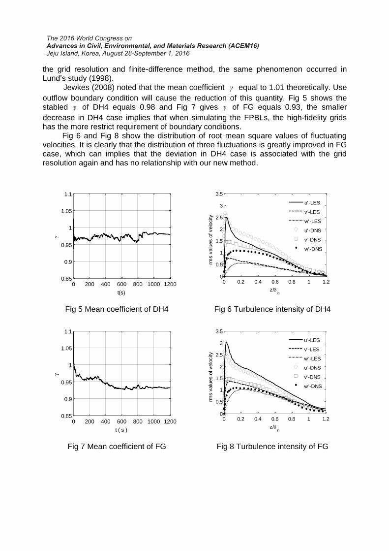
Jewkes (2008) noted that the mean coefficient γ equal to 1.01 theoretically. Use
outflow boundary condition will cause the reduction of this quantity. Fig 5 shows the stabled γ of DH4 equals 0.98 and Fig 7 gives γ of FG equals 0.93, the smaller
decrease in DH4 case implies that when simulating the FPBLs, the high-fidelity grids has the more restrict requirement of boundary conditions.
Fig 6 and Fig 8 show the distribution of root mean square values of fluctuating velocities. It is clearly that the distribution of three fluctuations is greatly improved in FG case, which can implies that the deviation in DH4 case is associated with the grid resolution again and has no relationship with our new method.
Fig 5 Mean coefficient of DH4 Fig 6 Turbulence intensity of DH4
Fig 7 Mean coefficient of FG Fig 8 Turbulence intensity of FG
0 200 400 600 800 1000 12000.85
0.9
0.95
1
1.05
1.1
t(s)
0 0.2 0.4 0.6 0.8 1 1.20
0.5
1
1.5
2
2.5
3
3.5
z/in
rms v
alu
es o
f velo
city
u-LES
v-LES
w-LES
u-DNS
v-DNS
w-DNS
0 200 400 600 800 1000 12000.85
0.9
0.95
1
1.05
1.1
t ( s )
0 0.2 0.4 0.6 0.8 1 1.20
0.5
1
1.5
2
2.5
3
3.5
z/in
rms v
alu
es o
f velo
city
u-LES
v-LES
w-LES
u-DNS
v-DNS
w-DNS

4.2 LES of non-smooth turbulent ABL up to Re=820000 Based on the optimal parameters achieved in section 4.1 and the performance of
our new recycling-rescaling method will be evaluated in this section. In CWE, the full scale and the wind-tunnel scale ABLs wind are frequently generated for comparison with field or experiment data. In this paper, we focus on the wind-tunnel scale wind generation. Unlike the smooth flat plate, most of earth surface is covered by various roughness elements, so two kinds of scaled turbulent ABLs over A and B terrain provided in China Loading Code (GB50009-2012) are set as targets. The detailed information of mean velocity and turbulence intensity profiles for A and B terrain is listed in Table 3.
Table 3 Target profiles of different terrain types
Terrain type Mean velocity Turbulence intensity
A
12.0
)(
δ
zUzU gradA
12.0
040.012.0)(
zzI A
B
15.0
)(
δ
zUzU gradB
15.0
034.014.0)(
zzIB
As shown in Fig 9, the size of the computational domain is: zyx LLL =14m3m
3.6m. For the convenient of comparison in the future, the height of computational domain is the same with the tunnel height of Wind Environmental Engineering laboratory of HITSZ. The recycle station is placed at 11.2m from the inlet. The simulated boundary layer thickness is δ =1.2m. The vertical height of computational
domain is 3 times of the boundary layer, which is enough to eliminate the effect of the
replaced top boundary conditions. The gradient velocity gradU =10m/s and gives the
Reynolds number
ν
δU gradRe 8.2105.
Fig 9 Computation Model of scaled turbulent ABLs
The grids divided uniformly in x and y directions and growing exponentially in z direction with growth factor 1.098. The first mesh height is 0.0001m, which satisfies
0.1Δ
wallz . The total grids number is zyx NNN =28050120=1680000.
The time step is 0.01s and the statistic time is the last 120s.
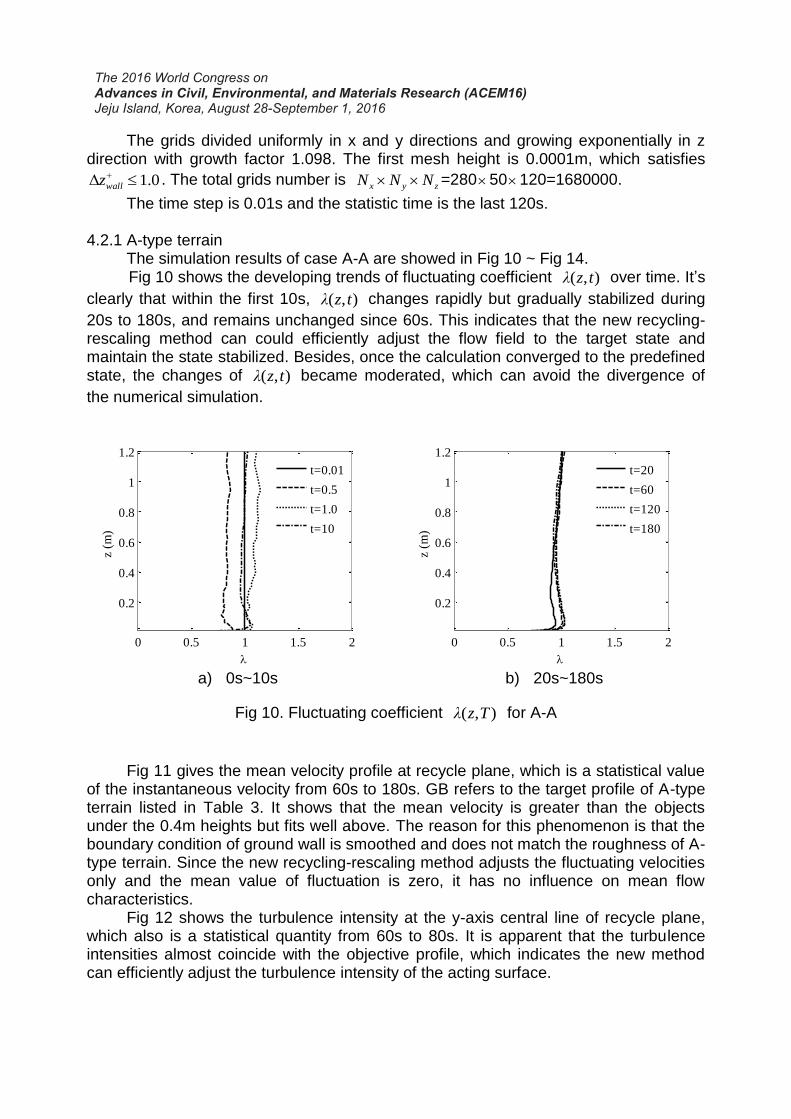
4.2.1 A-type terrain The simulation results of case A-A are showed in Fig 10 ~ Fig 14. Fig 10 shows the developing trends of fluctuating coefficient ),( tzλ over time. It’s
clearly that within the first 10s, ),( tzλ changes rapidly but gradually stabilized during
20s to 180s, and remains unchanged since 60s. This indicates that the new recycling-rescaling method can could efficiently adjust the flow field to the target state and maintain the state stabilized. Besides, once the calculation converged to the predefined state, the changes of ),( tzλ became moderated, which can avoid the divergence of
the numerical simulation.
a) 0s~10s b) 20s~180s
Fig 10. Fluctuating coefficient ),( Tzλ for A-A
Fig 11 gives the mean velocity profile at recycle plane, which is a statistical value
of the instantaneous velocity from 60s to 180s. GB refers to the target profile of A-type terrain listed in Table 3. It shows that the mean velocity is greater than the objects under the 0.4m heights but fits well above. The reason for this phenomenon is that the boundary condition of ground wall is smoothed and does not match the roughness of A-type terrain. Since the new recycling-rescaling method adjusts the fluctuating velocities only and the mean value of fluctuation is zero, it has no influence on mean flow characteristics.
Fig 12 shows the turbulence intensity at the y-axis central line of recycle plane, which also is a statistical quantity from 60s to 80s. It is apparent that the turbulence intensities almost coincide with the objective profile, which indicates the new method can efficiently adjust the turbulence intensity of the acting surface.
0 0.5 1 1.5 2
0.2
0.4
0.6
0.8
1
1.2
z (
m)
t=0.01
t=0.5
t=1.0
t=10
0 0.5 1 1.5 2
0.2
0.4
0.6
0.8
1
1.2
z (
m)
t=20
t=60
t=120
t=180
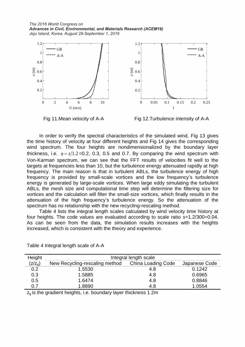
Fig 11.Mean velocity of A-A Fig 12.Turbulence intensity of A-A In order to verify the spectral characteristics of the simulated wind, Fig 13 gives
the time history of velocity at four different heights and Fig 14 gives the corresponding wind spectrum. The four heights are nondimensionalized by the boundary layer
thickness, i.e. 2.1zη =0.2, 0.3, 0.5 and 0.7. By comparing the wind spectrum with
Von-Karman spectrum, we can see that the FFT results of velocities fit well to the targets at frequencies less than 10, but the turbulence energy attenuated rapidly at high frequency. The main reason is that in turbulent ABLs, the turbulence energy of high frequency is provided by small-scale vortices and the low frequency’s turbulence energy is generated by large-scale vortices. When large eddy simulating the turbulent ABLs, the mesh size and computational time step will determine the filtering size for vortices and the calculation will filter the small-size vortices, which finally results in the attenuation of the high frequency’s turbulence energy. So the attenuation of the spectrum has no relationship with the new recycling-rescaling method.
Table 4 lists the integral length scales calculated by wind velocity time history at four heights. The code values are evaluated according to scale ratio s=1.2/300=0.04. As can be seen from the data, the simulation results increases with the heights increased, which is consistent with the theory and experience.
Table 4 Integral length scale of A-A
Height (z/zg)
Integral length scale New Recycling-rescaling method China Loading Code Japanese Code
0.2 1.5530 4.8 0.1242 0.3 1.5885 4.8 0.6965 0.5 1.6474 4.8 0.8846 0.7 1.8890 4.8 1.0554
zg is the gradient heights, i.e. boundary layer thickness 1.2m
0 2 4 6 8 10
0.2
0.4
0.6
0.8
1
1.2
U (m/s)
z (
m)
GB
A-A
0 0.05 0.1 0.15 0.2 0.25
0.2
0.4
0.6
0.8
1
1.2
I
z (
m)
GB
A-A

a)
b)
c)
d)
Fig 13.Velocity time history Fig 14. Wind spectrum
0 30 60 90 1204
6
8
10
12
t (s)
u (
m/s)
=0.2
10-1
100
101
102
10-4
10-2
100
n
nS
u/
u2
A-A =0.2
Von Karman
0 30 60 90 1204
6
8
10
12
t (s)
u (
m/s)
=0.3
10-1
100
101
102
10-4
10-2
100
n
nS
u/
u2
A-A =0.3
Von Karman
0 30 60 90 1206
8
10
12
14
t (s)
u (
m/s)
=0.5
10-1
100
101
102
10-4
10-2
100
n
nS
u/
u2
A-A =0.5
Von Karman
0 30 60 90 1206
8
10
12
14
t (s)
u (
m/s)
=0.7
10-1
100
101
102
10-4
10-2
100
n
nS
u/
u2
A-A =0.7
Von Karman

4.2.2 B-type terrain The simulation results of case B-A are showed in Fig 15~Fig 19. Fig 15 shows the developing trends of fluctuation coefficient ),( tzλ over time. It
clearly that the change of ),( tzλ for case B-A is the same with case A-A. This
indicates that the new recycling-rescaling method is also applicable for adjusting the turbulent ABL over B-type terrain which has certain roughness surface condition.
a) 0s~10s b) 20s~180s
Fig 15. Fluctuating coefficient ),( tzλ for B-A
Fig 16.Mean velocity of B-A Fig 17.Turbulent intensity of B-A Fig 16 gives the mean velocity profile at recycle plane. The evaluation of this
quantity is same with case A-A. GB refers to the target profile of B-type terrain in Table 3. It has the similar distribution with case A-A which means the methodology has no effects on mean flow characteristics.
0 0.5 1 1.5 2
0.2
0.4
0.6
0.8
1
1.2
z (
m)
t=0.01
t=0.5
t=1.0
t=10
0 0.5 1 1.5 2
0.2
0.4
0.6
0.8
1
1.2
z (
m)
t=20
t=60
t=181
0 2 4 6 8 10
0.2
0.4
0.6
0.8
1
1.2
U (m/s)
z (
m)
GB
B-A
0 0.1 0.2 0.3 0.4
0.2
0.4
0.6
0.8
1
1.2
I
z (
m)
GB
B-A

(a)
(b)
(c)
(d)
Fig 18.Velocity time history Fig 19. Wind spectrum
0 30 60 90 1204
6
8
10
12
t (s)
u (
m/s)
=0.2
10-1
100
101
102
10-4
10-2
100
n
nS
u/
u2
B-A =0.2
Von Karman
0 30 60 90 1204
6
8
10
12
t (s)
u (
m/s)
=0.3
10-1
100
101
102
10-4
10-2
100
n
nS
u/
u2
B-A =0.3
Von Karman
0 30 60 90 1206
8
10
12
14
t (s)
u (
m/s)
=0.5
10-1
100
101
102
10-4
10-2
100
n
nS
u/
u2
B-A =0.5
Von Karman
0 30 60 90 1206
8
10
12
14
t (s)
u (
m/s)
=0.7
10-1
100
101
102
10-4
10-2
100
n
nS
u/
u2
B-A =0.7
Von Karman
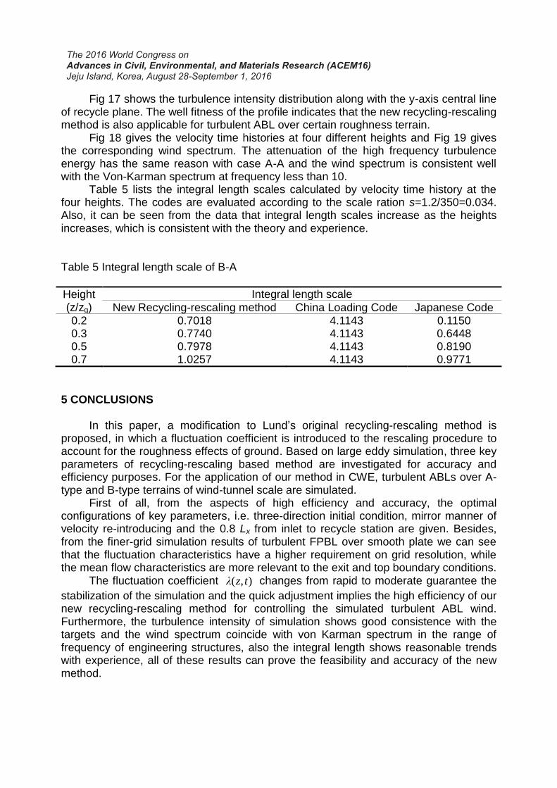
Fig 17 shows the turbulence intensity distribution along with the y-axis central line of recycle plane. The well fitness of the profile indicates that the new recycling-rescaling method is also applicable for turbulent ABL over certain roughness terrain.
Fig 18 gives the velocity time histories at four different heights and Fig 19 gives the corresponding wind spectrum. The attenuation of the high frequency turbulence energy has the same reason with case A-A and the wind spectrum is consistent well with the Von-Karman spectrum at frequency less than 10.
Table 5 lists the integral length scales calculated by velocity time history at the four heights. The codes are evaluated according to the scale ration s=1.2/350=0.034. Also, it can be seen from the data that integral length scales increase as the heights increases, which is consistent with the theory and experience.
Table 5 Integral length scale of B-A
Height (z/zg)
Integral length scale
New Recycling-rescaling method China Loading Code Japanese Code 0.2 0.7018 4.1143 0.1150 0.3 0.7740 4.1143 0.6448 0.5 0.7978 4.1143 0.8190 0.7 1.0257 4.1143 0.9771
5 CONCLUSIONS In this paper, a modification to Lund’s original recycling-rescaling method is
proposed, in which a fluctuation coefficient is introduced to the rescaling procedure to account for the roughness effects of ground. Based on large eddy simulation, three key parameters of recycling-rescaling based method are investigated for accuracy and efficiency purposes. For the application of our method in CWE, turbulent ABLs over A-type and B-type terrains of wind-tunnel scale are simulated.
First of all, from the aspects of high efficiency and accuracy, the optimal configurations of key parameters, i.e. three-direction initial condition, mirror manner of velocity re-introducing and the 0.8 Lx from inlet to recycle station are given. Besides, from the finer-grid simulation results of turbulent FPBL over smooth plate we can see that the fluctuation characteristics have a higher requirement on grid resolution, while the mean flow characteristics are more relevant to the exit and top boundary conditions.
The fluctuation coefficient ),( tzλ changes from rapid to moderate guarantee the
stabilization of the simulation and the quick adjustment implies the high efficiency of our new recycling-rescaling method for controlling the simulated turbulent ABL wind. Furthermore, the turbulence intensity of simulation shows good consistence with the targets and the wind spectrum coincide with von Karman spectrum in the range of frequency of engineering structures, also the integral length shows reasonable trends with experience, all of these results can prove the feasibility and accuracy of the new method.

Obviously, it cannot be denied that our new recycling-rescaling method has potential to be improved. Firstly, it is the mismatch of rough wall condition with the target ABL terrain that leads to the remarkable mismatch of mean velocity profile. In the present study, only the fluctuation velocity is rescaled to achieve the prescribed turbulence intensity, thus it is feasible to rescale the mean velocity to fit the targets as well. However, the fundamental approach to resolve this problem is to find an explicit relationship between the numerical rough wall condition and real rough terrain. Furthermore, the performance of our new method in simulating turbulent ABL over rougher terrain, such as D-type in the urban center, also need to be evaluated. ACKNOWLEDGEMENTS
The work described in this paper was supported by grants from Shenzhen
Science and technology Innovation Committee (Project No. JCYJ20130329154442496), HIT.NSRIF.2015086, and the National Natural Science Foundation of China (Project No. 51308167), which are gratefully acknowledged.
REFERENCE:
Jewkes, J. (2008). An Improved Turbulent Boundary Layer Inflow Condition, Applied to the Simulation of Jets in Cross-Flow, The University of Warwick. PhD. Kataoka, H. (2002). "Numerical flow computation around aeroelastic 3D square cylinder using inflow turbulence." wind and structures 5 (2~4): 379-392. Kataoka, H. (2008). "Numerical simulations of a wind-induced vibrating square cylinder within turbulent boundary layer." Journal of Wind Engineering and Industrial Aerodynamics 96 (10-11): 1985-1997. Lund, T. S. and X. Wu, et al. (1998). "Generation of Turbulent Inflow Data for Spatially-Developing Boundary Layer Simulations." Journal of Computational Physics 140 (2): 233-258. Nozawa, K. and T. Tamura (2001). Simulation of rough-wall turbulent boundary layer for LES inflow data. TSFP DIGITAL LIBRARY ONLINE, Begel House Inc.: 443. Nozawa, K. and T. Tamura (2002). "Large eddy simulation of the flow around a low-rise building immersed in a rough-wall turbulent boundary layer." Journal of Wind Engineering and Industrial Aerodynamics 90 (10): 1151-1162. Simens, M. P. and J. Jimenez, et al. (2007). A direct numerical simulation code for incompressible turbulent boundary layers, School of Aeronautics. Spalart, P. R. (1988). "Direct simulation of a turbulent boundary layer up toR,=1410." Journal of Fluid Mechanics 187: 61-98. Spalart, P. R. and M. Strelets, et al. (2006). "Direct numerical simulation of large-eddy-break-up devices in a boundary layer." International Journal of Heat and Fluid Flow 27 (5): 902-910.