large eddy simulation of unsteady turbulent flow in a semi

HAL Id: hal-01201416https://hal.archives-ouvertes.fr/hal-01201416

Submitted on 17 Sep 2015

HAL is a multi-disciplinary open accessarchive for the deposit and dissemination of sci-entific research documents, whether they are pub-lished or not. The documents may come fromteaching and research institutions in France orabroad, or from public or private research centers.

L’archive ouverte pluridisciplinaire HAL, estdestinée au dépôt et à la diffusion de documentsscientifiques de niveau recherche, publiés ou non,émanant des établissements d’enseignement et derecherche français ou étrangers, des laboratoirespublics ou privés.

Large eddy simulation of unsteady turbulent flow in asemi-industrial size spray dryer

F. Jongsma, F. Innings, M. Olsson, F. Carlsson

To cite this version:F. Jongsma, F. Innings, M. Olsson, F. Carlsson. Large eddy simulation of unsteady turbulent flow ina semi-industrial size spray dryer. Dairy Science & Technology, EDP sciences/Springer, 2013, 93 (4),pp.373-386. �10.1007/s13594-012-0097-y�. �hal-01201416�

https://hal.archives-ouvertes.fr/hal-01201416

https://hal.archives-ouvertes.fr

ORIGINAL PAPER

Large eddy simulation of unsteady turbulent flowin a semi-industrial size spray dryer

F. J. Jongsma & F. Innings & M. Olsson & F. Carlsson

Received: 23 September 2012 /Revised: 4 December 2012 /Accepted: 4 December 2012 /Published online: 10 January 2012# INRA and Springer-Verlag France 2012

Abstract This paper is concerned with the numerical simulation of gas flow insidespray dryers, which is known to be highly transient. Experimental evidence presented inthe literature to date is acquired either at a scale much smaller than industrial or at alimited number of locations in the system (e.g. the central axis). Alternatively, compu-tational fluid dynamics (CFD) simulation, in particular methods based on the Reynolds-averaged Navier–Stokes (RANS) equations, may provide the information of the com-plete flow field at industrial scales. However, RANS methods to some extent arehampered by the limitations of turbulence modelling. In this study, it has been investi-gated whether the current limitations of experiments and RANS CFD simulations can beomitted by the use of large eddy simulation (LES). The spray dryer studied was of semi-industrial size with a volume of 60m3. Via grid size and time step refinement studies, theminimum numerical requirements for obtaining converged time averaged velocityprofiles could be identified. Spectral analysis and estimates of the Kolmogorov scalesdemonstrated that LES resolves scales well into the inertial subrange of turbulencescales. The LES calculation shows a complex precession of the jet. The jet movesaround in the drying chamber seemingly with no reoccurring modes. Even with verylong sampling times, no typical frequencies could be found. This work demonstrates thefeasibility of LES for a spray dryer of semi-industrial scale and the ability of LES topredict large-scale motions. Future work will include the further validation of the LESvia comparison with laser Doppler anemometry measurements and, subsequently, thecomparison of RANS, unsteady RANS and LES simulations.

Keywords LES . CFD . Spray dryer . Transient flow

Dairy Sci. & Technol. (2013) 93:373–386DOI 10.1007/s13594-012-0097-y

F. J. Jongsma (*)Tetra Pak CPS, Venus 100, 8448 GW Heerenveen, The Netherlandse-mail: [email protected]

F. InningsTetra Pak Processing Systems, Ruben Rausings Gata, 221-86 Lund, Sweden

M. Olsson : F. CarlssonTetra Pak Packaging Solutions, Ruben Rausings Gata, 221-86 Lund, Sweden

1 Introduction

Computational fluid dynamics (CFD) simulation of the spray drying process hasreceived considerable attention, both in academia and industry, since the value ofmodelling as an aid in design of new systems, exploration of what-if scenarios ortroubleshooting studies (Fletcher et al. 2006) is recognised. In contrast to the decep-tively simple appearance of the technology, the physical processes taking place insidethe spray dryer are numerous, complex and highly coupled. In the present paper,some of the complexities of the air phase flow will be addressed.

The air flow inside spray dryers may be characterised as confined jet flow. Severalinvestigators (Usui et al. 1985; Kieviet et al. 1997; Godijn et al. 1999; Woo et al. 2009)have observed the confined jet may exhibit transient, large-scale motions. The term‘large’ here refers to the order of magnitude of the spray dryer itself. For example, the jetemanating from a central inlet in the roof of a spray dryer may deflect from the centralaxis towards the wall, and it may precess around the central axis. In contrast, the averagevelocity field of a free jet is axisymmetric and will exhibit steady-state behaviour. Oncethe jet is confined by walls, small deviations of the jet from the central axis may grow, ina self-sustained manner, and in turn continue to deflect the jet (Guo et al. 1998).

The observed transient flow patterns of the confined jet depend on: extent of swirlin the inlet flow (Southwell and Langrish 2001; Guo et al. 2001a), the Reynoldsnumber of the jet (Guo et al. 2001b) and the geometrical features of the system (Guoet al. 2001a, b, c). A map of flow regimes was presented by Guo et al. (2001b). Theregimes identified were termed, steady, transition, regular precession and complexprecession. The term steady refers to a flow regime closely resembling that of the freejet, but now with a stable toroidal flow structure around it. The steady regime isencountered when the walls are close to the jet, or expressed differently when theexpansion ratio, defined as the ratio of system and inlet diameters, is small. Uponincreasing the expansion ratio, a transitional regime may be observed before regularprecession is encountered.Moving the walls even further away from the central axis willresult in a regime change from regular to complex precession. In the latter regime, theprecession is no longer of constant amplitude and frequency but chaotic instead.

Early attempts to simulate the spray drying process were usually based on theassumptions of steady-state behaviour and axial symmetry, allowing for the use ofcomputationally less expensive 2D geometries. Currently, it is being acknowledged(Fletcher et al. 2006) that the predictive power of the CFD simulation of spray dryerswill benefit from considering full 3D geometries and transient simulations. Modellingefforts thus far have almost exclusively relied on solving the RANS equations inconjunction with the well known k-ε or k-ω based turbulence models. One exceptionwas reported by Fletcher and Langrish (2009), who applied the scale adaptivesimulation approach to the simulation of a pilot spray dryer. It appears that theapproaches that rely less on turbulence modelling, such as detached eddy simulationand large eddy simulation (LES) have not been explored yet.

Most experimental observations have been made on simple geometric systems(Dellenback et al. 1988, Hallet et al. 1984), e.g. a sudden expansion, or on spraydryers of laboratory size, up to spray dryers of approximately 1 m in diameter.Industrial spray dryers, especially for milk powder production, are usually an orderof magnitude bigger and consequently are operated at higher Reynolds numbers. The

374 F.J. Jongsma et al.

goal of this work is to investigate the flow features of a system that is closer to anindustrial size. Given the decrease in cost of computing power LES has been used.The present report is aimed firstly at demonstrating the feasibility of LES simulationof a spray dryer of semi-industrial scale and secondly at an initial exploration of largescale features of the flow in this system. Future work will include further validation ofthe LES model results by comparison with measured data.

2 Methods

2.1 System

The spray dryer studied is presented in Fig. 1. The pilot spray dryer is of thecylinder on cone type, with cylindrical dimensions of 3.8 m diameter and 4.1 mheight and a cone top angle of 43°, resulting in a total volume of 60 m3. Air isfed through an annular gap in the roof and it escapes the dryer through four topoutlets. The inlet is annular due to the fact that a pipe with a diameter of0.103 m is located on the vertical axis of the dryer where normally finepowder is fed for the purpose of agglomeration. The inlet diameter of thedryer is 0.437 m and the expansion ratio 8.7. For the simulations, the outletswere simplified as indicated in Fig. 1. The Reynolds number of the jet, based ona feed rate of 6,440 kg h−1 and the air inlet diameter was 5.105.

Fig. 1 Pilot Tetra Pak-widebody spray dryer

Large eddy simulation of unsteady turbulent flow 375

2.2 Simulation set-up and procedure

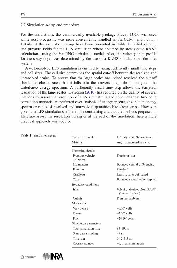
For the simulations, the commercially available package Fluent 13.0.0 was usedwhile post processing was more conveniently handled in StarCCM+ and Python.Details of the simulation set-up have been presented in Table 1. Initial velocityand pressure fields for the LES simulation where obtained by steady-state RANScalculations, using the k-ε RNG turbulence model. Also, the velocity inlet profilefor the spray dryer was determined by the use of a RANS simulation of the inletsystem.

A well-resolved LES simulation is ensured by using sufficiently small time stepsand cell sizes. The cell size determines the spatial cut-off between the resolved andunresolved scales. To ensure that the large scales are indeed resolved the cut-offshould be chosen such that it falls into the universal equilibrium range of theturbulence energy spectrum. A sufficiently small time step allows the temporalresolution of the large scales. Davidson (2010) has reported on the quality of severalmethods to assess the resolution of LES simulations and concludes that two pointcorrelation methods are preferred over analysis of energy spectra, dissipation energyspectra or ratios of resolved and unresolved quantities like shear stress. However,given that LES simulations still are time consuming and that the methods proposed inliterature assess the resolution during or at the end of the simulation, here a morepractical approach was adopted.

Table 1 Simulation set-upTurbulence model LES, dynamic Smagorinsky

Material Air, incompressible 25 °C

Numerical details

Pressure–velocitycoupling

Fractional step

Momentum Bounded central differencing

Pressure Standard

Gradients Least squares cell based

Time Bounded second order implicit

Boundary conditions

Inlet Velocity obtained from RANS(Vortex method)

Outlets Pressure, ambient

Mesh sizes

Very coarse ~1.106 cells

Coarse ~7.106 cells

Fine ~24.106 cells

Simulation parameters

Total simulation time 80–190 s

Start data sampling 40 s

Time step 0.12–0.5 ms

Courant number ~1, in all simulations


To allow for sufficiently small residuals, proper convergence was ensured inseveral ways. Firstly, the courant number of the calculations was kept below (butclose) to one. Secondly, three combinations of grid size and time step refinementswere tested to ensure independency on both parameters. Finally, the grid cell and timestep sizes where compared with estimates of the Kolmogorov scales of turbulenceobtained from the steady state RANS simulations. Estimates of the Kolmogorovscales are obtained from RANS simulations, via the turbulence energy dissipationrate, ε. Their significance with respect to the judgement of the resolution will beexplained below.

2.3 Data sampling, treatment and interpretation

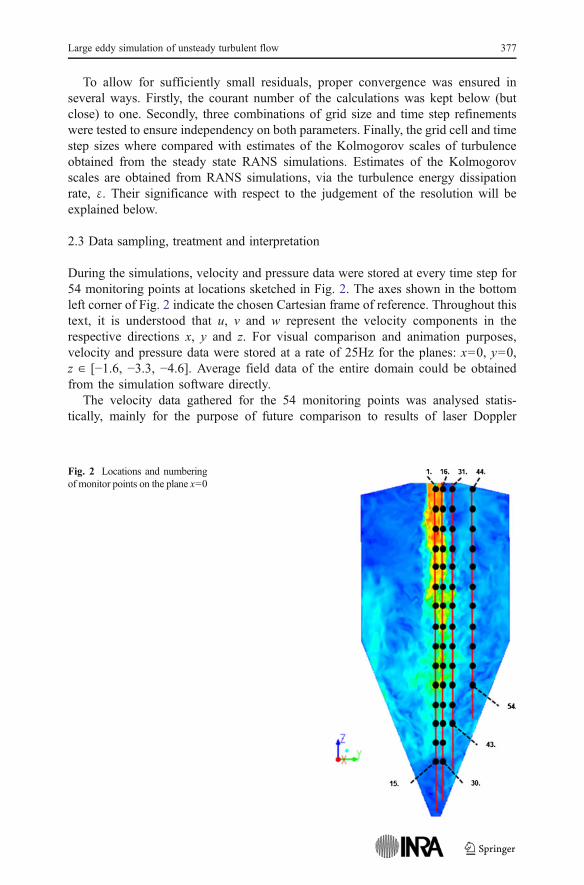
During the simulations, velocity and pressure data were stored at every time step for54 monitoring points at locations sketched in Fig. 2. The axes shown in the bottomleft corner of Fig. 2 indicate the chosen Cartesian frame of reference. Throughout thistext, it is understood that u, v and w represent the velocity components in therespective directions x, y and z. For visual comparison and animation purposes,velocity and pressure data were stored at a rate of 25Hz for the planes: x=0, y=0,z ∈ [−1.6, −3.3, −4.6]. Average field data of the entire domain could be obtainedfrom the simulation software directly.

The velocity data gathered for the 54 monitoring points was analysed statis-tically, mainly for the purpose of future comparison to results of laser Doppler

Fig. 2 Locations and numberingof monitor points on the plane x=0


anemometry measurements. The individual point velocity–time signals obtainedwere subjected to Fourier transformation for the construction of power spectraldensities (PSD), to reveal possible dominant frequencies associated with certainscales of the turbulent structures.

Further investigation of flow patterns was conducted by applying a low-passfilter to the frequency signal of the velocity fluctuations, u′, v′ and w′. Thevelocity fluctuations were obtained by subtracting the average from the actualvelocity. The time signal of the velocity fluctuation was then reconstructed fromthe Fourier components of the low frequencies. For several points, the filteredcross-sectional (u′, v′) velocity fluctuations where plotted in the form of a so-called phase space plot. A similar method was proposed earlier by Guo et al.(2001b, 2003) for the identification of periodicity in the results of transientRANS simulations.

Compared with the case of interpreting results of transient RANS calculations,here a choice needs to be made on the frequency that is used for filtering. Dependingon the exact choice, different patterns may arise in the phase space plot making directcomparison troublesome. The significance of the phase space plot however lies morein the fact whether or not patterns that may appear are regular or not. Hence,regardless of the exact choice of filtering frequency, phase space plots will revealeither periodicity or irregularity.

3 Results and discussion

3.1 Visualisation of the flow field

Contour plots of the instantaneous velocity field (Fig. 3) demonstrated the time-dependent motions in the flow field. Detectable motions of the flow ranged from roll-up vortices, typical for the shear layer of the jet, up to more complex movements ofthe entire jet.

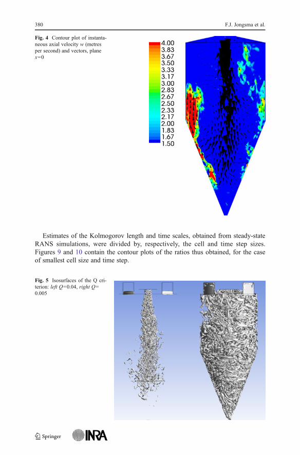
Visual inspection of animations, constructed from the contour plots of the hori-zontal planes (z∈ [−1.6, −3.3, and −4.6]), revealed a gradual breakdown of the jetstructure upon deeper entering the dryer. At a height of −1.6 m, the jet was stilllocated centrally in the dryer, circular in shape and nearly invariant in axial velocity.Deeper into the spray dryer, e.g. z=−4.6, the shape of the jet was observed to bestretched, deflected from the central axis and no longer exhibited a spatially flatvelocity profile, see Fig. 3. Large-scale motions in the space surrounding the jet couldbe observed in animations constructed from the contour plots of the vertical planes. Itappeared that movement of the jet towards the wall was often accompanied bystrong gusts of flow on the opposite wall. These gusts of higher upwardvelocity started at approximately half the height of the cone and could extendas far as up to the roof of the dryer. In Fig. 4, one example of the observedgusts is presented as combined contour (w) and vector plot, indicating theinstantaneous velocities.

The structure of the turbulence was visualised by iso-surfaces of the Q criterion asshown in Fig. 5. The Q criterion is a scalar quantity that is defined as Q=0.5⋅(Ω2–S2),where Ω is the vorticity magnitude and S the mean strain rate. If at a certain location


in the flow the Q criterion is positive, this indicates that the rotation dominates thestrain and shear.

The time-averaged velocity magnitude and the turbulence kinetic energy fields,shown in Figs. 6 and 7, respectively, appeared to be symmetric. The symmetry ofboth fields is an indication that the total simulation time was several times more thanthe time-scale of transient flow structures.

The contour plot of the average velocity field (Fig. 6) further supported theobservations made from the animations that there are frequent gusts of upward flowalongside the walls. Inside the conical section, the average flow field of the jet isdirectly surrounded by an area of low average velocity, which in turn is surroundedby an area of higher, upward velocity.

3.2 Convergence tests

In Fig. 8, the downward directed, axial velocity component w, is plotted as afunction of dimensionless axial distance (based on inlet diameter) for the threecombinations of cell and time step sizes. To avoid repetition similar plots, e.g.the radial velocity profiles, are omitted. It was noted, however, that the (timeaveraged) LES solution indeed converged upon cell size and time steprefinement.

Fig. 3 Contour plots of velocity magnitude (top, middle) and axial velocity components, w, (bottom) forthe planes: x=0 (top), y=0 (middle) and z=−4.6 (bottom), at times counted from the start of data collection(i.e. t>40 s)


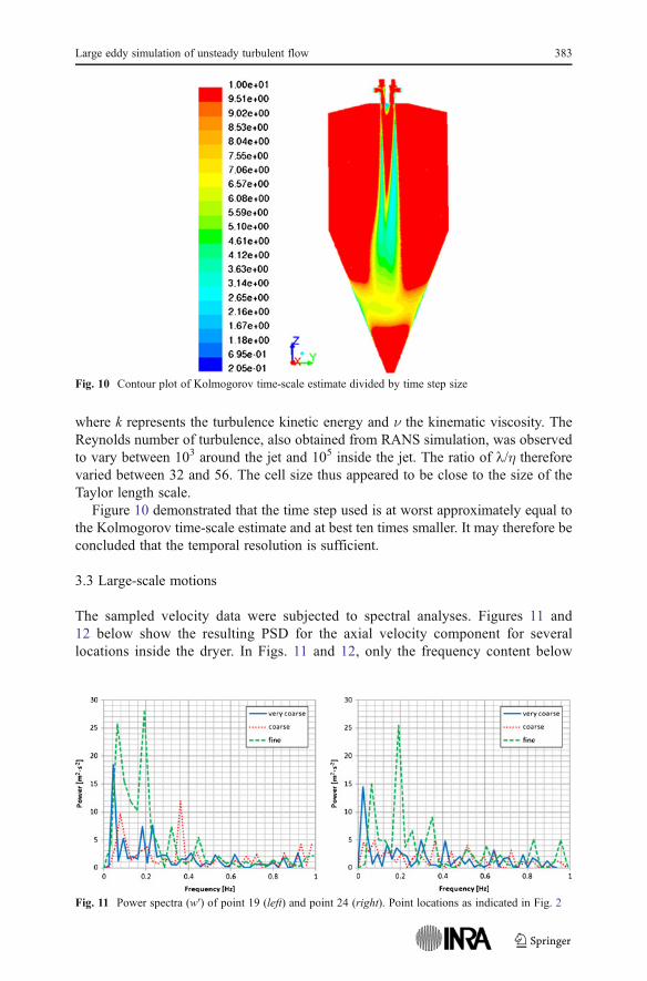
Estimates of the Kolmogorov length and time scales, obtained from steady-stateRANS simulations, were divided by, respectively, the cell and time step sizes.Figures 9 and 10 contain the contour plots of the ratios thus obtained, for the caseof smallest cell size and time step.

Fig. 4 Contour plot of instanta-neous axial velocity w (metresper second) and vectors, planex=0

Fig. 5 Isosurfaces of the Q cri-terion: left Q=0.04, right Q=0.005


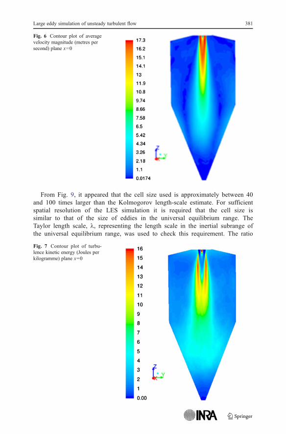
From Fig. 9, it appeared that the cell size used is approximately between 40and 100 times larger than the Kolmogorov length-scale estimate. For sufficientspatial resolution of the LES simulation it is required that the cell size issimilar to that of the size of eddies in the universal equilibrium range. TheTaylor length scale, 1, representing the length scale in the inertial subrange ofthe universal equilibrium range, was used to check this requirement. The ratio

Fig. 6 Contour plot of averagevelocity magnitude (metres persecond) plane x=0

Fig. 7 Contour plot of turbu-lence kinetic energy (Joules perkilogramme) plane x=0


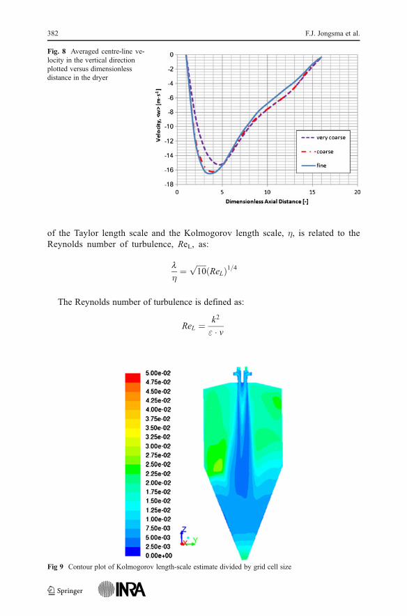
of the Taylor length scale and the Kolmogorov length scale, η, is related to theReynolds number of turbulence, ReL, as:

lη¼

ffiffiffiffiffi

10p

ðReLÞ1=4

The Reynolds number of turbulence is defined as:

ReL ¼ k2

" � v

Fig. 8 Averaged centre-line ve-locity in the vertical directionplotted versus dimensionlessdistance in the dryer

Fig 9 Contour plot of Kolmogorov length-scale estimate divided by grid cell size


where k represents the turbulence kinetic energy and ν the kinematic viscosity. TheReynolds number of turbulence, also obtained from RANS simulation, was observedto vary between 103 around the jet and 105 inside the jet. The ratio of 1/η thereforevaried between 32 and 56. The cell size thus appeared to be close to the size of theTaylor length scale.

Figure 10 demonstrated that the time step used is at worst approximately equal tothe Kolmogorov time-scale estimate and at best ten times smaller. It may therefore beconcluded that the temporal resolution is sufficient.

3.3 Large-scale motions

The sampled velocity data were subjected to spectral analyses. Figures 11 and12 below show the resulting PSD for the axial velocity component for severallocations inside the dryer. In Figs. 11 and 12, only the frequency content below

Fig. 10 Contour plot of Kolmogorov time-scale estimate divided by time step size

Fig. 11 Power spectra (w′) of point 19 (left) and point 24 (right). Point locations as indicated in Fig. 2


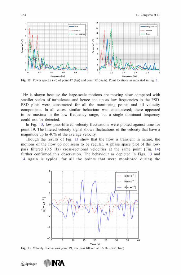
1Hz is shown because the large-scale motions are moving slow compared withsmaller scales of turbulence, and hence end up as low frequencies in the PSD.PSD plots were constructed for all the monitoring points and all velocitycomponents. In all cases, similar behaviour was encountered; there appearedto be maxima in the low frequency range, but a single dominant frequencycould not be detected.

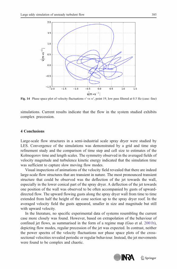
In Fig. 13, low pass-filtered velocity fluctuations were plotted against time forpoint 19. The filtered velocity signal shows fluctuations of the velocity that have amagnitude up to 40% of the average velocity.

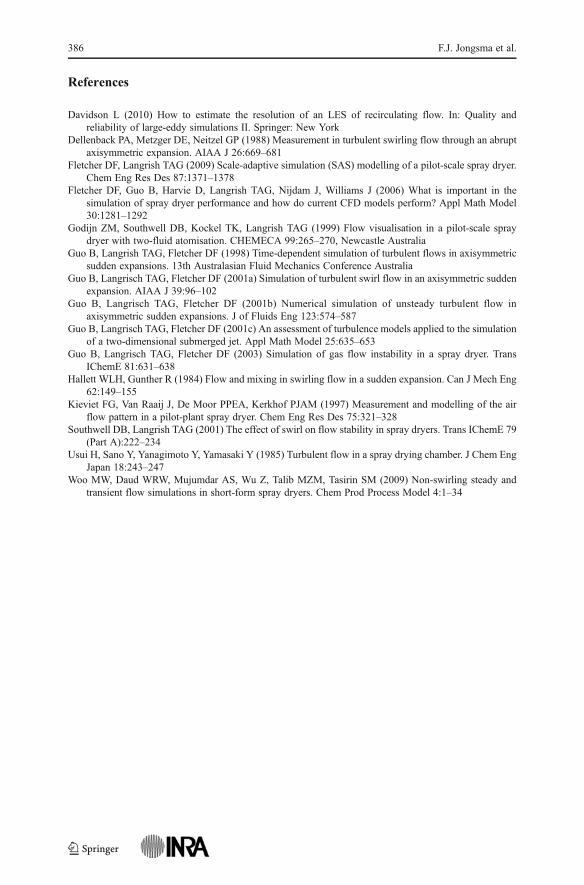
Though the results of Fig. 13 show that the flow is transient in nature, themotions of the flow do not seem to be regular. A phase space plot of the low-pass filtered (0.5 Hz) cross-sectional velocities at the same point (Fig. 14)further confirmed this observation. The behaviour as depicted in Figs. 13 and14 again is typical for all the points that were monitored during the

Fig. 12 Power spectra (w′) of point 47 (left) and point 52 (right). Point locations as indicated in Fig. 2

Fig. 13 Velocity fluctuations point 19, low pass filtered at 0.5 Hz (case: fine)


simulations. Current results indicate that the flow in the system studied exhibitscomplex precession.

4 Conclusions

Large-scale flow structures in a semi-industrial scale spray dryer were studied byLES. Convergence of the simulations was demonstrated by a grid and time steprefinement study and the comparison of time step and cell size to estimates of theKolmogorov time and length scales. The symmetry observed in the averaged fields ofvelocity magnitude and turbulence kinetic energy indicated that the simulation timewas sufficient to capture slow moving flow modes.

Visual inspections of animations of the velocity field revealed that there are indeedlarge-scale flow structures that are transient in nature. The most pronounced transientstructure that could be observed was the deflection of the jet towards the wall,especially in the lower conical part of the spray dryer. A deflection of the jet towardsone position of the wall was observed to be often accompanied by gusts of upward-directed flow. The upward flowing gusts along the spray dryer wall from time to timeextended from half the height of the cone section up to the spray dryer roof. In theaveraged velocity field the gusts appeared, smaller in size and magnitude but stillwith upward velocity.

In the literature, no specific experimental data of systems resembling the currentcase more closely was found. However, based on extrapolation of the behaviour ofconfined jet flows, as summarised in the form of a regime map (Guo et al. 2001b),depicting flow modes, regular precession of the jet was expected. In contrast, neitherthe power spectra of the velocity fluctuations nor phase space plots of the cross-sectional velocities revealed periodic or regular behaviour. Instead, the jet movementswere found to be complex and chaotic.

Fig. 14 Phase space plot of velocity fluctuations v′ vs w′, point 19, low pass filtered at 0.5 Hz (case: fine)


References

Davidson L (2010) How to estimate the resolution of an LES of recirculating flow. In: Quality andreliability of large-eddy simulations II. Springer: New York

Dellenback PA, Metzger DE, Neitzel GP (1988) Measurement in turbulent swirling flow through an abruptaxisymmetric expansion. AIAA J 26:669–681

Fletcher DF, Langrish TAG (2009) Scale-adaptive simulation (SAS) modelling of a pilot-scale spray dryer.Chem Eng Res Des 87:1371–1378

Fletcher DF, Guo B, Harvie D, Langrish TAG, Nijdam J, Williams J (2006) What is important in thesimulation of spray dryer performance and how do current CFD models perform? Appl Math Model30:1281–1292

Godijn ZM, Southwell DB, Kockel TK, Langrish TAG (1999) Flow visualisation in a pilot-scale spraydryer with two-fluid atomisation. CHEMECA 99:265–270, Newcastle Australia

Guo B, Langrish TAG, Fletcher DF (1998) Time-dependent simulation of turbulent flows in axisymmetricsudden expansions. 13th Australasian Fluid Mechanics Conference Australia

Guo B, Langrisch TAG, Fletcher DF (2001a) Simulation of turbulent swirl flow in an axisymmetric suddenexpansion. AIAA J 39:96–102

Guo B, Langrisch TAG, Fletcher DF (2001b) Numerical simulation of unsteady turbulent flow inaxisymmetric sudden expansions. J of Fluids Eng 123:574–587

Guo B, Langrisch TAG, Fletcher DF (2001c) An assessment of turbulence models applied to the simulationof a two-dimensional submerged jet. Appl Math Model 25:635–653

Guo B, Langrisch TAG, Fletcher DF (2003) Simulation of gas flow instability in a spray dryer. TransIChemE 81:631–638

Hallett WLH, Gunther R (1984) Flow and mixing in swirling flow in a sudden expansion. Can J Mech Eng62:149–155

Kieviet FG, Van Raaij J, De Moor PPEA, Kerkhof PJAM (1997) Measurement and modelling of the airflow pattern in a pilot-plant spray dryer. Chem Eng Res Des 75:321–328

Usui H, Sano Y, Yanagimoto Y, Yamasaki Y (1985) Turbulent flow in a spray drying chamber. J Chem EngJapan 18:243–247

Woo MW, Daud WRW, Mujumdar AS, Wu Z, Talib MZM, Tasirin SM (2009) Non-swirling steady andtransient flow simulations in short-form spray dryers. Chem Prod Process Model 4:1–34


Southwell DB, Langrish TAG (2001) The effect of swirl on flow stability in spray dryers. Trans IChemE 79(Part A):222–234

large eddy simulation of unsteady turbulent flow in a semi

Documents