a novel approach to fuzzy soft sets in decision making based on … · theory, mycin certainty...

Received 9 January 2015

Accepted 7 August 2015

A novel approach to fuzzy soft sets in decision making based on grey relationalanalysis and MYCIN certainty factor

Ningxin Xie 1 Yu Han 2 Zhaowen Li 2 ∗

1 College of Information Science and Engineering, Guangxi University for Nationalities, Nanning, Guangxi530006, P.R.China

E-mail:[email protected] College of Science, Guangxi University for Nationalities, Nanning, Guangxi 530006, P.R.China

E-mail:[email protected], [email protected]

Abstract

This paper proposes a novel approach to decision making based on grey relational analysis and MYCINcertainty factor, which describes decision making problems with fuzzy soft sets. Firstly, we utilize grey re-lational analysis to obtain the grey mean relational degree, and the uncertain degree of various parametersis acquired. On the basis of uncertain degree, we obtain the essence uncertainty factor of each inde-pendent alternative with each parameter. Information can be fused in accordance with MYCIN certaintyfactor combination rule and the best alternatives are achieved. By using three examples, comparing withthe mean potentiality approach and giving an application to medical diagnosis problems, the feasibilityand effectiveness of the approach are demonstrated.

Keywords: Fuzzy soft set; Decision making; Grey relational analysis; MYCIN certainty factor.

1. Introduction

To solve complicated problems in economics, engi-

neering, environmental science and social science,

methods in classical mathematics are not always

successful because of the existence of various types

of uncertainties. There are several theories: prob-

ability theory, fuzzy set theory46, rough set theory37 and interval mathematics which we can consider

as mathematical tools to deal with uncertainties. But

all these theories have their own limitations 31 which

present many difficulties. To overcome these diffi-

culties, a new approach was proposed in 31, which is

called soft set theory for dealing with uncertainty.

Recently, there has been a rapid growth of inter-

est in soft set theory. Maji et al. 32,34 further dis-

cussed soft set theory and defined fuzzy soft sets

by combining soft sets with fuzzy sets. The study

of hybrid models combining soft sets or fuzzy soft

sets with other mathematical structures and new op-

erations is emerging as an active research topic of

soft set theory10,19,45. Aktas et al. 1 initiated soft

groups. Jun et al. 16,17 applied soft sets to BCK/BCI-

algebras. Feng et al. 10 defined soft semirings

and established the connection between soft sets and

semirings. Jiang et al. 19 extended soft sets with

description logics. Li et al. 27,28 considered rough-

ness of fuzzy soft sets and obtained the relationship

∗Corresponding author: Zhaowen Li

International Journal of Computational Intelligence Systems, Vol. 8, No. 5 (2015) 959-976

Co-published by Atlantis Press and Taylor & FrancisCopyright: the authors

959

Ningxin Xie, Yu Han, Zhaowen Li

among soft sets, soft rough sets and topologies. Li

et al. 30 studied parameter reductions of soft cov-

erings. Nowadays, soft set theory has been proved

to be useful in many kinds of fields, such as rule

mining15, simulation21, forecasting 43, data analysis51 and decision making 3,23,38.

Maji et al. 35 first applied soft sets to solve de-

cision making problems with the help of rough set

approaches. Chen et al. 5 defined the parameters

reduction of soft sets and discussed its application

of decision making problem. Cagman et al. 3,4 pre-

sented soft matrix theory and uni-int decision mak-

ing approach, which selected a set of optimum ele-

ments from different alternatives. Roy et al. 38 dis-

cussed score value as the evaluation basis to find an

optimal choice object in fuzzy soft sets. Feng et al.9 pointed out the limitation of Roy’s method and ap-

plied level soft sets to discuss fuzzy soft sets based

on decision making. Jiang et al. 18 presented an ad-

justable approach to intuitionistic fuzzy soft sets 33

based on decision making by using level soft sets of

intuitionistic fuzzy soft sets. Basu et al. 2 further

compared the previous methods to fuzzy soft sets in

decision making and introduced the mean potential-

ity approach, which showed more efficient and more

accurate than the previous.

The unique or uniform criterion does not exist for

the selection on the above approaches to fuzzy soft

sets in decision making. Although researchers focus

on a direction as the evaluation basis, such as choice

value, score value or others, the same decision mak-

ing problem may obtain different results from using

various evaluation bases. As a result, it is difficult

to judge which result is better and which method

should be chosen for selecting the optimal choice

object. The key to this problem is how to reduce

subjectivity and uncertainty. Then it is necessary to

pay attention to this issue.

Grey relational analysis method is important to

reflect uncertainty in grey system theory initiated by

Deng 6, which is utilized for generalizing estimates

under small samples and uncertain conditions. Liu24 further develop the theory. And it has been suc-

cessfully applied in solving decision making prob-

lems 22,42,50. Certainty factor has been proposed

by Shortliffe and Buchanan 39 and then applied in

MYICIN expert system 40. Then Heckerman 7 de-

veloped it. It is a powerful method for combining ac-

cumulative evidences of changing prior opinions in

the light of new evidences. Compared to probability

theory, MYCIN certainty factor captures more in-

formation to support decision making by identifying

the uncertain and unknown evidence. It provides the

mechanism to derive solutions from various vague

evidences without knowing much prior information.

The advantage of this model is more intuitive and

easier to master, its algorithm is simpler and the less

amount of calculation. Moreover, it avoids the prior

probability or priori possibility problems in proba-

bility or possibility theory. MYCIN certainty factor

has been successfully applied into many fields such

as intelligent medical diagnosis, earthquake predic-

tion and program design 25,40. Decision makers are

able to take full advantage of both methods’ merits

to deal with uncertainty and risk confidently by com-

bining both above theories. Thus, it not only avoids

the problem of selecting the suitable level soft sets

to obtain choice values and score values, but also re-

duces uncertainty caused by people’s subjective cog-

nition so as to raise the choice decision level. And

the application to medical diagnosis problems show

that the hybrid model is effective and practical under

uncertain conditions.

The remaining part of this paper is organized as

follows. In Section 2, we present some concepts

about fuzzy soft sets and MYCIN certainty factor. In

Section 3, we recall the mean potentiality approach

to fuzzy soft sets in decision making and give three

examples to illustrate this approach. In Section 4,

we apply grey relational analysis to determine the

uncertain degree of each parameter, by which suit-

able essence uncertainty factor with respect to each

parameter is constructed. And we do decision mak-

ing by using MYCIN certainty factor combination

rule. In Section 5, we give measure of performance

and the interpretations of the results. In Section 6,

we demonstrate the feasibility of new approach by

comparing with the mean potentiality approach and

giving an application to medical diagnosis problems.

In Section 7, we end this paper with some conclu-

sions.


960

Fuzzy soft sets in decision making

2. Preliminaries

Throughout this paper, U denotes an initial universe,

E denotes the set of all possible parameters and IU

denotes the set of all fuzzy subsets of U . We only

consider the case where U and E are both nonempty

finite sets.

In this section, we recall some basic concepts

about fuzzy soft sets and MYCIN certainty factor.

2.1. Fuzzy soft sets

Definition 2.1 (32) Let A ⊆ E. A pair (F,A) iscalled a fuzzy soft set over U, where F is a mappinggiven by F : A → IU .

In other words, a fuzzy soft set is a parametrized

family of fuzzy sets in the universe. For each e ∈ A.

F(e) is a fuzzy set in U and is called a fuzzy set with

respect to the parameter e.

Denote U = {h1,h2, . . . ,hm} and A ={e1,e2, . . . ,en}. Put

gi j = F(e j)(hi).

Then G = (gi j)m×n is called the fuzzy soft matrix

induced by (F,A).It is easy to see that every soft set may be con-

sidered as a fuzzy soft set 9.

Example 2.2 Let (F,A) be a fuzzy soft setover U where U = {h1,h2,h3,h4,h5} and A ={e1,e2,e3,e4,e5,e6}, defined as follows:

F(e1) =0.8h1

+ 1h2+ 0.2

h3+ 0.3

h4+ 1

h5,

F(e2) =0.5h1

+ 0.1h2

+ 0.3h3

+ 0.2h4

+ 0.1h5,

F(e3) =0.1h1

+ 0.4h2

+ 1h3+ 1

h4+ 0.8

h5,

F(e4) =0h1+ 0.3

h2+ 0.1

h3+ 1

h4+ 0

h5,

F(e5) =0.6h1

+ 0h2+ 1

h3+ 0.3

h4+ 0.7

h5,

F(e6) =0.1h1

+ 0.4h2

+ 0.7h3

+ 1h4+ 0.2

h5.

Then (F,A) is described by Table 1.

Table 1: Tabular representation of the fuzzy soft

set(F,A)h1 h2 h3 h4 h5

e1 0.8 1 0.2 0.3 1

e2 0.5 0.1 0.3 0.2 0.1

e3 0.1 0.4 1 1 0.8

e4 0 0.3 0.1 1 0

e5 0.6 0 1 0.3 0.7

e6 0.1 0.4 0.7 1 0.2

If h is viewed as an assumption(or object), then

F(e)(h) may represent the degree that the parameter

e holds the object h and F(e)c(h) may represent the

degree that the parameter e opposes the object h.

Obviously, F(e)(h)+F(e)c(h) = 1.

Definition 2.3 Let A ⊆ E and let (F,A) be a fuzzysoft set over U. Se(h) =F(e)(h)−F(e)c(h) is calledthe score function value of h with respect to e.

The score function represents the difference be-tween the support degree and the opposite degree.Especially, when Se(h) = 1, it expresses the param-eter e is all for the object h; Se(h) = −1, it ex-presses the parameter e totally against to the objecth; Se(h) = 0, it expresses the same degree of the pa-rameter e support or opposite the object h.

Denote U = {h1,h2, . . . ,hm} and A ={e1,e2, . . . ,en}. Put

si j = F(e j)(hi)−F(e j)c(hi).

Then S = (si j)m×n is called the score matrix inducedby (F,A).

Definition 2.4 (32) Let A,B ⊆ E and let (F,A) and(G,B) be two fuzzy soft sets over U. (F,A) is a fuzzysoft subset of (G,B) if

(i) A ⊆ B,(ii) F(e) is a fuzzy subset of G(e) for any e ∈ A.We denote it by (F,A) ⊂ (G,B) or

(G,B) ⊃ (F,A), at this point, (G,B)is said to bea fuzzy soft super set of (F,A).

It is obvious that (F,A) = (G,B) if and only if

(F,A) ⊂ (G,B) and (F,A) ⊃ (G,B).

Definition 2.5 (32) Let A,B ⊆ E and let (F,A) ,(G,B) be two fuzzy soft sets over U. Then “ (F,A)AND (G,B) ” is a fuzzy soft set denoted by (F,A)∧(G,B) and is defined by (F,A)∧(G,B) = (H,A×B),where H(α,β ) = F(α)∩G(β ) for α ∈ A and β ∈ B,


961


where ∩ is the operation “fuzzy intersection” of twofuzzy sets.

2.2. MYCIN certainty factor

Certainty factor’s reliability is an imprecise reason-

ing model used by MYCIN system, it is a reason-

able and effective inference model in many practi-

cal applications. MYCIN certainty factor is a new

important inference method under uncertainty con-

ditions. It has an advantage to deal with subjective

judgments and to synthesize the uncertainty knowl-

edge 49.

In this paper, CF(e) represents the confidence

degree of the evidence e when the evidence e is un-

certain as true, its value is in [−1,1]. The larger

value of CF(e), the higher credibility of the evi-

dence e. Specially, CF(e) = 1 means the evidence

e is true; CF(e) =−1 means the evidence e is fake.

Definition 2.6 (49) Let h be a random variable ofassumptions and let e be a random variable of ev-idences. Then CF(h/e) = MB(h/e)−MD(h/e) iscalled MYCIN certainty factor, where

MB(h/e) =

{P(h/e)∨P(h)−P(h)

1−P(h) , P(h) �= 1;

1, P(h) = 1;

MD(h/e) =

{P(h)−P(h/e)∧P(h)

P(h) , P(h) �= 0;

1, P(h) = 0.

MB(h/e) is called the degree of confidence in

growth which means the increase confidence level

of the assumption h at the emergence of evidence

e; MD(h/e) is called the degree of no-confidence in

growth which means the decrease confidence level

of the assumption h at the emergence of evidence e.

CF(h/e) means the confidence degree of the as-

sumption h is true in case of the evidence e, its value

is in [−1,1]. Especially, when CF(h/e) = 1, it ex-

presses assumption h is true in case of the evidence

e; CF(h/e) = −1, it expresses assumption h is fake

in case of the evidence e; CF(h/e) = 0, it expresses

assumption h could not determine in case of the ev-

idence e.

Definition 2.7 (26) Let h be a random variable ofassumption and let e be a random variable of evi-dence. If the evidence e is uncertain as true, thenthe essence uncertainty factor is defined as:

CFT (h/e) =CF(h/e) ·CF(e).

CFT (h/e) represents the confidence degree of theassumption h is true while the confidence degree ofevidence e is CF(e).

In reality, decision makers can often gain access

to more than one information source for the sake of

making decisions. Therefore, we introduce the fol-

lowing definitions. The generation function which

can be synthesized constructs the synthetic function

of the essence uncertainty factor from these infor-

mation sources. And then we get the evidence syn-

thesis formula. This construction is called MYCIN

certainty factor combination rule for group aggrega-

tion.

Definition 2.8 (49) A function F : [0,∞)→ [−1,1] iscalled a generation function, if F be satisfied the fol-lowing two conditions:

(1) F(0) =−1,F(∞) =−1, F(x)is monotone in-creasing;

(2) F(1/x) =−F(x).Definition 2.9 (49) The generation function F :

[0,∞)→ [−1,1] is called to be synthesized, if thereis a function of two variables f such that F(x · y) =f (F(x),F(y)).Theorem 2.10 (49) Suppose that e1 and e2 are con-ditional independence about h and h. F is a gener-ation function which can be synthesized. The gener-ation function of the essence uncertainty factor is asfollows:

CFT (h/e1,e2) = F(P(e1,e2/h)P(e1,e2/h)

).

It means that there is a function f :

[−1,1]2 → [−1,1] such that CFT (h/e1,e2) =f (CFT (h/e1),CFT (h/e2)).

Because

F1(x · y) = F1(x)+F1(y)1+F1(x) ·F1(y)

is a kind of generation function which can be syn-

thesized, then the evidence synthesis formula is as

follows:


962


CFT (h/e1,e2) =CFT (h/e1)+CFT (h/e2)

1+CFT (h/e1) ·CFT (h/e2).

The synthesis of multiple evidences can be pro-

moted according to MYCIN certainty factor combi-

nation rule:Suppose that e1,e2, · · ·,em are conditional inde-

pendence about h and h. F is a generation functionwhich can be synthesized. The generation functionof the essence uncertainty factor is as follows:

CFT (h/e1,e2, · · ·,em) = f (CFT (h/e1,e2, · · ·,em−1),CFT (h/em)).

That is,

CFT (h/e1,e2, · · ·,em) =CFT (h/e1,e2, · · ·,em−1)+CFT (h/em)

1+CFT (h/e1,e2, · · ·,em−1) ·CFT (h/em).

MYCIN certainty factor combination rule can in-

crease the confidence degree and reduce the uncer-

tain degree of the whole evidences to improve relia-

bility.

Example 2.11 Let E = {e1,e2} be the set of evi-dences. Suppose there are two different assumptionsh1 and h2 over E, induced by an independent pieceof evidences e1,e2, given by

CFT (h1/e1) = 0.2, CFT (h1/e2) = 0.7,CFT (h2/e1) = 0.4, CFT (h2/e2) = 0.3.Combining the two evidences by MYCIN cer-

tainty factor combination rule leads to:

CFT (h1/e1,e2) =CFT (h1/e1)+CFT (h1/e2)

1+CFT (h1/e1) ·CFT (h1/e2)

=0.2+0.7

1+0.2×0.7= 0.7895,

CFT (h2/e1,e2) =CFT (h2/e1)+CFT (h2/e2)

1+CFT (h2/e1) ·CFT (h2/e2)

=0.4+0.3

1+0.4×0.3= 0.4117.

3. Mean potentiality approach

Just as most of the decision making problems, fuzzy

soft sets based on decision making involve the eval-

uation of all decision alternatives. Recently, appli-

cations of fuzzy soft sets based on decision making

have attracted more and more attentions. The works

of Roy et al. 9,20,38 are fundamental and significant.

Later Kong et al. 23 applied grey relational analysis

to solve fuzzy soft sets in decision making. Gener-

ally, there does not exist any unique or uniform cri-

terion for the evaluation of decision alternatives un-

der uncertain conditions. Thus, Basu et al. 2 further

studied and proposed the mean potentiality approach

to fuzzy soft sets in decision making, which is more

deterministic and accurate than Feng’s approach 9.

Below, we introduce Basu’s approach.

Let U = {h1,h2, · · · ,hm} be the universe and A ={e1,e2, · · · ,en} be a set of parameters. Given a fuzzy

soft set (F,A). We mainly recall the mean poten-

tiality approach to (F,A) based on decision making

problems with equally weighted choice parameters:

Step 1. Find a normal parameter reduction B of

A 36. If it exists, we construct the tabular represen-

tation of (F,B). Otherwise, we construct the tabu-

lar representation of (F,A) with the choice values of

each object.

Step 2. Compute the mean potentiality mp =∑m

i=1 ∑nj=1 F(e j)(hi)

m×n up to ρ significant figures, denoted

by m′p.

Step 3. Construct a m′p-level soft set of (F,A) and

represent it in tabular form, then compute the choice

value ci for each hi.

Step 4. Denote max {c1,c2, · · · ,cm}=ck. If ck is

unique, then the optimal choice object is hk and the

process will be stopped. Otherwise, go to Step 5.

Step 5. Compute the non-negative difference be-

tween the largest and the smallest membership value

in each column (resp. each row) and denote it as α j( j = 1,2, · · · ,n) (resp. βi (i = 1,2, · · · ,m)).

Step 6. Compute the average α =∑n

j=1 a j

n up to ρsignificant figures, denoted by α ′.

Step 7. Construct a α ′-level soft set of (F,A) and

represent it in tabular form, then compute the choice

value c′i for each hi.

Step 8. Denote max {c′1,c

′2, · · · ,c

′m}=c

′l . If c

′l is

unique, then the optimal choice object is hl and the

process will be stopped. Otherwise, go to Step 9.

Step 9. Consider the object corresponding to the

minimum value of βi (i = 1,2, · · · ,m) as the optimal

choice of decision makers.

The following examples illustrate the mean po-


963


tentiality approach to fuzzy soft sets in decision

making. Firstly, we give an example which can be

stopped at Step 4.

Example 3.1 Let us consider a decision makingproblem which is associated with the fuzzy soft set(F,A) given in Table 2.

(1) Since A is indispensable, there does not existany normal parameter reduction of A.

(2) Since the mean potentiality of (F,A) is mp =∑3

i=1 ∑3j=1 F(e j)(hi)

3×3= 0.655, then m′

p = 0.6.(3) m′

p-level soft set of (F,A) with choice valuesis given by Table 3.

(4) Since max {ci, i = 1,2,3} = c2, then the op-timal choice is h2.

Table 2: Tabular representation of (F,A)e1 e2 e3

h1 0.8 0.7 0.2

h2 0.6 0.9 0.7

h3 0.7 0.5 0.8

Table 3: Tabular representation of L((F,A),0.6)with choice values

e1 e2 e3 Choice valueh1 1 1 0 2

h2 1 1 1 3

h3 1 0 1 2

Secondly, we give another example which can be

stopped at Step 9.




i=1 ∑5j=1 F(e j)(hi)

3×5= 0.622, then m′

p = 0.62.(3) m′


(4) Since h1 and h2 have the same maximumchoice values (3), we have to calculate the α j andβi values of (F,A).

(5) See Table 6.(6) Now α = 0.29+0.27+0.56+0.32+0.32

5= 0.352,

thus α ′ = 0.35.(7) So the α ′-level soft set of (F,A) with choice

values c′i (i = 1,2,3) is given by Table 7.

(8) Here max {c′1,c

′2,c

′3} = {c

′2,c

′3} ( i.e., not

unique), we have to consider the β2 and β3.(9) Since min{β2,β3} = β3(= 0.37), then h3 is

the optimal choice object.

Table 4: Tabular representation of (F,A)e1 e2 e3 e4 e5

h1 0.85 0.73 0.26 0.32 0.75

h2 0.56 0.82 0.76 0.64 0.43

h3 0.84 0.55 0.82 0.53 0.47


e1 e2 e3 e4 e5 Choice valueh1 1 1 0 0 1 3

h2 0 1 1 1 0 3

h3 1 0 1 0 0 2

Table 6: Tabular representation of (F,A) with αi and

β j values

e1 e2 e3 e4 e5 βih1 0.85 0.73 0.26 0.32 0.75 0.59

h2 0.56 0.82 0.76 0.64 0.43 0.39

h3 0.84 0.55 0.82 0.53 0.47 0.37

αi 0.29 0.27 0.56 0.32 0.32


e1 e2 e3 e4 e5 Choice valueh1 1 1 0 0 1 3

h2 1 1 1 1 1 5

h3 1 1 1 1 1 5

We can apply the mean potentiality approach to

deal with the above two cases. Now, we consider the

following example.




i=1 ∑5j=1 F(e j)(hi)

3×5= 0.7455, then m′

p = 0.74.(3) m′


(4) Since h1 and h2 have the same maximumchoice values (3), we have to calculate the α j andβi values of (F,A).

(5) See Table 10


964


(6) Now α = 0.2+0.4+0.43

= 0.3333, thus α ′ =0.33.

(7) So the α ′-level soft set of (F,A) with choicevalues c

′i (i = 1,2,3) is given by Table 11.

(8) Here max {c′1,c

′2,c

′3} = {c

′2,c

′3} ( i.e., not

unique), we have to consider the β2 and β3.(9) Since β2 = β3(= 0.30), h2 or h3 is the opti-

mal choice object.

Table 8: Tabular representation of (F,A)e1 e2 e3

h1 0.89 0.79 0.29

h2 0.69 0.99 0.79

h3 0.79 0.59 0.89



h2 0 1 1 2

h3 1 0 1 2

Table 10: Tabular representation of (F,A) with αi

and β j values

e1 e2 e3 βih1 0.89 0.79 0.29 0.60

h2 0.69 0.99 0.79 0.30

h3 0.79 0.59 0.89 0.30

αi 0.2 0.4 0.4



h2 1 1 1 3

h3 1 1 1 3

By Basu’s approach, decision makers can not de-

cide which one is the optimal choice object. Now

we try to overcome this problem by proposing a new

approach for decision making problem of fuzzy soft

sets as follows.

4. A novel approach to fuzzy soft sets indecision making based on grey relationalanalysis and MYCIN certainty factor

The existing approaches to fuzzy soft sets in deci-

sion making are mainly based on the level soft set

to obtain useful information such as choice values

and score values. However, it is very difficult for

decision makers to select a suitable level soft set.

Now we introduce a new approach to fuzzy soft sets

in decision making based on grey relational analysis

and MYCIN certainty factor. The approach is effec-

tive and practical under uncertain conditions. It not

only allows us to avoid the problem of selecting the

suitable level soft set, but also helps reducing uncer-

tainty caused by people’s subjective cognition so as

to raise the choice decision level.

This approach include three phases: First, grey

relational analysis is applied to calculate the grey

mean relational degree between each independent

alternative and the mean of all alternatives with each

parameter, and the uncertain degree of each param-

eter is obtained. Second, the suitable essence uncer-

tainty factor with respect to each parameter (or evi-

dence) is constructed by the uncertain degree of each

parameter. Third, we apply MYCIN certainty fac-

tor combination rule to aggregate independent evi-

dences into a collective evidence, by which the can-

didate alternatives are ranked and the best alterna-

tive(s) are obtained. The stepwise procedure of this

approach is described in Fig. 1.

4.1. The approach

In this paper, regard the solution system of decision

making system as a set of different assumptions and

treat the target system as a set of evidences.

In the following, we consider a decision mak-

ing problem concerned with m different assumptions

and n different evidences (or parameters), and we al-

ways denote

U = {h1,h2, · · · ,hm}, A = {e1,e2, · · · ,en}.

Let (F,A) be a fuzzy soft set over U and let

G = (gi j)m×n be the fuzzy soft matrix induced by

(F,A).Compared to the score function Se(h) and

MYCIN certainty factor CF(h/e), both are very

similar in the sense, so we can substitute Se(h) for

CF(h/e), it means that CF(hi/e j) = si j.

Compared to probability theory, MYCIN cer-

tainty factor captures more information to support

decision making, by identifying the uncertain and


965


Figure 1: Flow chart of algorithm.

unknown evidences. It provides a mechanism to de-

rive solutions from various vague evidences with-

out knowing much prior information. The primary

problem is how to obtain the uncertain degree of ev-

idences.

First we present some basic notions.

Definition 4.1 (41) Let (F,A) be a fuzzy soft set overU. Suppose that G = (gi j)m×n and S = (si j)m×n arerespectively the fuzzy soft matrix and the score ma-trix induced by (F,A). For any i, j, denote

si =1

n

n

∑j=1

si j, si j = |si j − si|,

ri j =min1�i�m si j +ρ max1�i�m si j

si j +ρ max1�i�m si j,

where ρ ∈ (0,1),

DOI(e j) =1

m(

m

∑i=1

(ri j)q)

1q .

Then(1) si is called the mean of all parameters with

respect to hi,(2) si j is called the difference information be-

tween si j and si,(3) ρ is called the distinguishing coefficient and

ri j is called the grey mean relational degree betweensi j and si,

(4) DOI(e j) is called the q order uncertain de-gree of the parameter e j.

In this paper we pick ρ = 0.5, q= 2 and just con-

sider grey mean relational degree between si j and si29.

MYCIN certainty factor is a powerful tool

for combining accumulative evidences of changing

prior opinions in the light of new evidences 49. The


966


primary procedure about combining the known ev-

idences or information with other evidences is to

construct suitable essence uncertainty factor. It is

flexible to obtain MYCIN certainty factor. People’s

experience, knowledge or thinking will affect the se-

lection of MYCIN certainty factor.

Now, by the uncertain degree of each parameter,

we can obtain production function of each assump-

tion with respect to each parameter.

Definition 4.2 Let (F,A) be a fuzzy soft set over U.Suppose that G = (gi j)m×n and S = (si j)m×n are re-spectively the fuzzy soft matrix and score matrix in-duced by (F,A).

PutCF(e j) = 1−DOI(e j),

CFT (hi/e j) =CF(hi/e j) ·CF(e j)

= si j (1−DOI(e j)),

CF = (CF(hi/e j))m×n,

CFT = (CFT (hi/e j))m×n.

Then CF(e j) is called the certain degree of theparameter e j, CFT (hi/e j) is called the essence un-certainty factor of the assumption hi in case of theevidence e j, and CF and CFT are respectively calledthe MYCIN certainty factor matrix and essence un-certainty factor matrix induced by (F,A).

Based on the above analysis, an approach to the

fuzzy soft set (F,A) in decision making based on

grey relational analysis and MYCIN certainty factor

can be summarized as follows:

Step 1. Construct the fuzzy soft matrix G =(gi j)m×n induced by (F,A).

Step 2. Construct the soft matrix S = (si j)m×ninduced by (F,A) and the MYCIN certainty factor

matrix CF induced by (F,A).Step 3. Calculate the mean of all parameters with

respect to each assumption by

si =1

n

n

∑j=1

si j.

Step 4. Calculate the difference information be-

tween si j and si and construct the difference matrix

by

si j = |si j − si|, S = ( si j)m×n.

Step 5. Calculate the gray mean relational degree

between si j and si by

ri j =min1�i�m si j +0.5 max1�i�m si j

si j +0.5 max1�i�m si j.

Step 6. Calculate the uncertain degree of the pa-

rameter e j by

DOI(e j) =1

m(

m

∑i=1

(ri j)2)

12 .

Step 7. Calculate the certain degree CF(e j) of

the parameter e j by Definition 4.2.

Step 8. Construct the essence uncertainty factor

matrix CFT induced by (F,A).Step 9. Calculate the confidence degree of each

assumption hi by combining these evidences respec-

tively by Theorem 2.10. Obtain decision making.

The decision is hk if hk = max CFT (hi/e j)). Opti-

mal choices have more than one object if there are

more assumptions corresponding to the maximum.

4.2. Example illustration

In this subsection, we give the following examples

to illustrate new approach to fuzzy soft sets in deci-

sion making.

Example 4.3 Using new approach, we reconsiderthe fuzzy soft set (F,A) given in Examples 3.1.

We suppose that the universe U = {h1,h2,h3} asa set of different assumptions and the set of param-eters A = {e1,e2,e3} as a set of evidences. The pro-cess is as follows:

(1) Construct the fuzzy soft matrix G = (gi j)m×ninduced by (F,A) as follows:

G = (gi j)3×3 =

⎛⎝ 0.8 0.7 0.20.6 0.9 0.70.7 0.5 0.8

⎞⎠ .

(2) Construct the MYCIN certainty factor matrixas follows:

CF = (si j)3×3 =

⎛⎝ 0.6 0.4 −0.60.2 0.8 0.40.4 0 0.6

⎞⎠ .


967


(3) Calculate the mean of all parameters of eachassumption hi as follows:

s1 = 0.1333, s2 = 0.4667, s3 = 0.3333.

(4) Calculate the difference information betweensi j and si, and construct the difference matrix as fol-lows:

S =

⎛⎝ 0.4667 0.2667 0.7333

0.2667 0.3333 0.0667

0.0667 0.3333 0.2667

⎞⎠ .

(5) Calculate the gray mean relational degreebetween si j and si based on S as follows:

(ri j)3×5 =

⎛⎝ 0.4286 1.0000 0.3939

0.6000 0.8667 1.0000

1.0000 0.8667 0.6842

⎞⎠ .

(6) Calculate the uncertain degree of each pa-rameter e j as follows:

DOI(e1) = 0.4141,

DOI(e2) = 0.5273,

DOI(e3) = 0.4247.

(7) Calculate the certain degree of each param-eter e j as follows:

CF(e1) = 0.5859,

CF(e2) = 0.4727,

CF(e3) = 0.5753.

(8) Construct the essence uncertainty factor ma-trix CFT as follows:

CFT =

⎛⎝ 0.3515 0.1891 −0.3452

0.1172 0.3782 0.2301

0.2343 0 0.3452

⎞⎠ .

(9) Calculate the confidence degree of each as-sumption hi by combining these evidences respec-tively as follows:

CFT (h1/e1,e2,e3) = 0.1960,

CFT (h2/e1,e2,e3) = 0.6351,

CFT (h3/e1,e2,e3) = 0.5362.

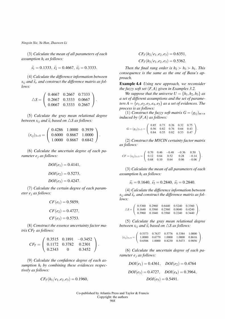
Then the final rang order is h2 � h3 � h1. Thisconsequence is the same as the one of Basu’s ap-proach.Example 4.4 Using new approach, we reconsiderthe fuzzy soft set (F,A) given in Examples 3.2.

We suppose that the universe U = {h1,h2,h3} asa set of different assumptions and the set of parame-ters A = {e1,e2,e3,e4,e5} as a set of evidences. Theprocess is as follows:

(1) Construct the fuzzy soft matrix G = (gi j)m×ninduced by (F,A) as follows:

G = (gi j)3×3 =

⎛⎝ 0.85 0.73 0.26 0.32 0.75

0.56 0.82 0.76 0.64 0.43

0.84 0.55 0.82 0.53 0.47

⎞⎠ .

(2) Construct the MYCIN certainty factor matrixas follows:

CF = (si j)3×5 =

⎛⎝ 0.70 0.46 −0.48 −0.36 0.50

0.12 0.64 0.52 0.28 −0.14

0.68 0.10 0.64 0.06 −0.06

⎞⎠ .


s1 = 0.1640, s2 = 0.2840, s3 = 0.2840.


S =

⎛⎝ 0.5360 0.2960 0.6440 0.5240 0.3360

0.1640 0.3560 0.2360 0.0040 0.4240

0.3960 0.1840 0.3560 0.2240 0.3440

⎞⎠ .


(ri j)3×5 =

⎛⎝ 0.5373 0.7637 0.5776 0.3384 1.0000

1.0000 0.6779 1.0000 1.0000 0.8616

0.6506 1.0000 0.8230 0.5473 0.9856

⎞⎠ .


DOI(e1) = 0.4361, DOI(e2) = 0.4764

DOI(e3) = 0.4727, DOI(e4) = 0.3964,

DOI(e5) = 0.5491.


968



CF(e1) = 0.5639, CF(e2) = 0.5236,

CF(e3) = 0.5273. CF(e4) = 0.6036,

CF(e5) = 0.4509.

(8) Construct the essence uncertainty factor ma-trix as follows:

CFT =

⎛⎝ 0.3947 0.2408 −0.2531 −0.2173 0.2254

0.0677 0.3351 0.2742 0.1690 −0.0631

0.3834 0.0524 0.3375 0.0362 −0.0271

⎞⎠ .


CFT (h1/e1,e2,e3) = 0.3909,

CFT (h2/e1,e2,e3) = 0.6669,

CFT (h3/e1,e2,e3) = 0.6734.

Then the final rang order is h3 � h2 � h1.Thisconsequence is also the same as the one of Basu’sapproach.

Examples 4.3 and 4.4 illustrate that new ap-

proach is reasonable.

To address the issue in Example 3.3 we apply

new approach. Matching process is as follows:

Example 4.5 We suppose that the universe U ={h1,h2,h3} as a set of different assumptions and theset of parameters A = {e1,e2,e3} as a set of evi-dences. The process is as follows:

(1) Construct the fuzzy soft matrix G = (gi j)m×ninduced by (F,A).

G = (gi j)3×3 =

⎛⎝ 0.89 0.79 0.29

0.69 0.99 0.79

0.79 0.59 0.89

⎞⎠ .

(2) Construct the MYCIN certainty factor matrixinduced by (F,A).

CF = (si j)3×5 =

⎛⎝ 0.78 0.58 −0.42

0.38 0.98 0.58

0.58 0.18 0.7800

⎞⎠ .


s1 = 0.3133, s2 = 0.6467, s3 = 0.5133,


S =

⎛⎝ 0.4667 0.2667 0.7333

0.2667 0.3333 0.0667

0.0667 0.3333 0.2667

⎞⎠ .


(ri j)3×5 =

⎛⎝ 0.4286 1.0000 0.3939

0.6000 0.8667 1.0000

1.0000 0.8667 0.6842

⎞⎠ .


DOI(e1) = 0.4141,

DOI(e2) = 0.5273,

DOI(e3) = 0.4247,


CF(e1) = 0.5859,

CF(e2) = 0.4727,

CF(e3) = 0.5753.

(8) Construct the essence uncertainty factor ma-trixinduced by (F,A).

CFT =

⎛⎝ 0.4570 0.2742 −0.2416

0.2226 0.4633 0.3337

0.3398 0.0851 0.4487

⎞⎠ .



969


CFT (h1/e1,e2,e3) = 0.4841,

CFT (h2/e1,e2,e3) = 0.7913,

CFT (h3/e1,e2,e3) = 0.7270.

Then the final rang order is h2 � h3 � h1. Con-sidering the former examples, we can push out thisconsequence is reasonable.

5. Measure of performance and theinterpretations of the results

Definition 5.1 (2) Let M be a method which satis-fies n parameters optimality criteria based on fuzzysoft set. Let F(ei)(Op) be the degree of the optimalobject Op support the parameters ei. Let

ζ ijk = |F(ei)(Op)−F(e j)(Op)|

ϒM =1

n∑

i=1

n∑

j=1,i�= jζ i

jk

+n

∑i=1

F(ei)(Op),

ζ ijk is called the non-negative differences between

the parameters ei and the parameters e j, ϒM iscalled the measure of performance of method M.

Let M1 and M2 be two methods which satisfythe optimality criteria based on fuzzy soft set, theirmeasure of performances are ϒM1

and ϒM2. Now,

if ϒM1> ϒM2

then method ϒM1is better than ϒM2

;on the contrary, method ϒM2

is better than ϒM1; if

ϒM1= ϒM2

then the two method have the same per-formance.

We have gain the substantial uncertainty factors

of assumption hi through the above analysis, as for

the complexity of objective facts and the limitation

of people’s realization, for the problems in reality,

there is overall uncertainty condition, so this paper

propose a method to obtain the substantial uncer-

tainty factors of overall uncertainty.

Considering that the substantial uncertainty fac-

tors of each assumption hi are induced by fuzzy soft

set (F,A). Then we can define the un-belief degree

of real assumption hi as follows:

CFcT (hi/e1,e2, · · · ,e j)

=

{1−CFT (hi/e1,e2, · · · ,e j), CFT (hi/e1,e2, · · · ,e j)� 0;

1+CFT (hi/e1,e2, · · · ,e j), CFT (hi/e1,e2, · · · ,e j)< 0.

The uncertainty degree of hi after evidence synthe-sis is

CFU (hi/e1,e2, ...,e j) =CFT (hi/e1,e2, ...,e j)−CFcT (hi/e1,e2, ...,e j).

Definition 5.2

CFU =1

m

m

∑i=1

CFU(hi/e1,e2, ...,e j)

is called the substantial uncertainty factors of over-all uncertainty.

Consider Example 3.3. We have

CFT (h1/e1,e2,e3) = 0.1960,

CFT (h2/e1,e2,e3) = 0.6351,

CFT (h3/e1,e2,e3) = 0.5362;

CFcT (h1/e1,e2,e3) = 0.8040,

CFcT (h2/e1,e2,e3) = 0.3649,

CFcT (h3/e1,e2,e3) = 0.4638.

Calculate

CFU(h1/e1,e2,e3) =−0.6080,

CFU(h2/e1,e2,e3) = 0.2702,

CFU(h3/e1,e2,e3) = 0.0724.

Then

1

3

3

∑i=1

CFU(hi/e1,e2,e3) = 0.3168.

Calculate the substantial uncertainty factors of

overall uncertainty by mean potentiality approach:

1

3

3

∑i=1

CFT (hi/e1,e2,e3) = 0.4557.

By the definition, we calculate that the measure

of performances by new approach and the mean po-

tentiality approach are both ϒ = 3.8667.

Briefly, the comparison results of above ap-

proaches are shown in the following table.


970


Table 12: The comparison results of the substantial

uncertainty factors of overall uncertainty

Decision-making method Result ranking CFU ϒMean potentiality approach h2 � h3 � h1 0.4557 3.8667

New approach h2 � h3 � h1 0.3168 3.8667

Analysis the results of above table, the value of

the substantial uncertainty factors of overall uncer-

tainty lower from the initial average 0.4557 to the

combined 0.3168.

Consider Example 3.2.2. We have

CFT (h1/e1,e2,e3,e4,e5) = 0.3909,

CFT (h2/e1,e2,e3,e4,e5) = 0.6669,

CFT (h3/e1,e2,e3,e4,e5) = 0.6734;

CFcT (h1/e1,e2,e3) = 0.6091,

CFcT (h2/e1,e2,e3) = 0.3331,

CFcT (h3/e1,e2,e3) = 0.3264.

Then

1

3

3

∑i=1

CFU(hi/e1,e2,e3) = 0.1542.



1

3

3

∑i=1

CFT (hi/e1,e2,e3) = 0.5770.

By the definition, we can calculate that the mea-

sure of performances by new approach and the mean

potentiality approach are both ϒ = 3.6954.Briefly, the comparison results of above ap-




Decision-making method Result ranking CFU ϒMean potentiality approach h3 � h2 � h1 0.5770 3.6954

New approach h3 � h2 � h1 0.1542 3.6954




combined 0.1542.

Consider Example 3.2.3. We have

CFT (h1/e1,e2,e3) = 0.4841,

CFT (h2/e1,e2,e3) = 0.7913,

CFT (h3/e1,e2,e3) = 0.7270;

CFcT (h1/e1,e2,e3) = 0.5159,

CFcT (h2/e1,e2,e3) = 0.2087,

CFcT (h3/e1,e2,e3) = 0.2730.

Then

1

3

3

∑i=1

CFU(hi/e1,e2,e3) = 0.3349.



1

3

3

∑i=1

CFT (hi/e1,e2,e3) = 0.6674.

By the definition, we can calculate that the mea-

sure of performances by new approach and the mean

potentiality approach are both ϒ = 4.1366.





Decision-making method Result ranking CFU ϒMean potentiality approach h2 = h3 � h1 0.6674 4.1366

New approach h2 � h3 � h1 0.3349 4.1366




combined 0.3349.

The three examples above illustrate that new ap-

proach can significantly reduce the perception of un-

certainty. Moreover, the measure of performances

reflect the effectiveness of the new method.


971


6. An application for medical diagnosisproblems

One of the toughest challenges in medical diagno-

sis is handling uncertainty. Doctors always detect

clinical manifestations by the comparison with pre-

defined classes to find the most similar disease. Only

one comprehensive result can be gotten from ex-

isting methods for medical diagnosis, which can-

not provide the certainty or uncertainty of the result.

Therefore, we do not know how to deal with the un-

known factors in the process of medical diagnosis.

In the section, we apply new approach to solve the

medical diagnosis problem.

Now we consider the medical diagnosis problem

cited from Examples 6.2 which is investigated by

Basu et al. 2.

Suppose that the universe U contains four dis-

eases, given by

U = {acute dental abscess, migraine, acute sinusi-

tis, peritonsillar abscess}= {d1,d2,d3,d4}(say).

And the set of parameters E is given by

E = {fever, runningnose, weakness, oro-

facial pain, nausea vomiting, swelling, trismus, his-

tory, physical examination, laboratory investigation}= {e1,e2,e3,e4,e5,e6,e7,s1,s2,s3}(say).

Let A, B be two subsets of E given by A ={e1,e2,e3,e4,e5,e6,e7} and B = {s1,s2,s3}. Sup-

pose that (F,A) and (G,B) are two fuzzy soft sets

describing “ symptoms of the diseases ” and “ deci-

sion making tools of the diseases ”, respectively.

We believe the authors of the literature 2 have in-

vestigated some data and processed the data in Ex-

amples 6.2. And they get the tabular representation

of (F,A) and (G,B), which are given in Tables 12

and 13, respectively. In view of the rationality of the

data, and in order to make better contrast with new

approach, we quote the the tabular representation in

Table 12 and 13.

Now suppose that a patient who is suffering from

a disease has three symptoms as follows: fever,

running nose, oro-facial pain, which is denoted by

P = e1,e2,e4. The key problem is how a doc-

tor reaches to the most suitable diagnosis accord-

ing to the symptoms, history, physical examina-

tion and laboratory investigation of the patient. To

solve this problem, we consider “ (F,A) ∧ (G,B)”, given by Table 14. There are four diseases

d1, d2, d3, d4, and nine pairs of parameters a1 =(e1,s1),a2 =(e1,s2),a3 =(e1,s3),a4 =(e2,s1),a5 =(e2,s2),a6 =(e2,s3),a7 =(e4,s1),a8 =(e4,s2),a9 =(e4,s3), which is a pair of one symptom and one de-

cision making tool, respectively.

Table 15: Tabular representation of the fuzzy soft set

(F,A)e1 e2 e3 e4 e5 e6 e7

d1 0.6 0 0.6 0.9 0 0.7 0.8

d2 0.2 0 0.1 0.9 0.8 0 0

d3 0.3 0.7 0.3 0.8 0.3 0.4 0

d4 0.4 0 0.2 0.7 0.1 0.6 0.5

Table 16: Tabular representation of the fuzzy soft set

(G,B)s1 s2 s3

d1 0.6 0.8 0.4

d2 0.8 0.3 0.6

d3 0.8 0.4 0.7

d4 0.6 0.8 0.3

Next we will apply new approach to detect

which disease is most suited with the symptoms

and these investigative procedures. Then, in the

making decision, we consider that the four dis-

eases construct a set of different assumptions, de-

noted by D = {d1,d2,d3,d4}. and the nine pairs

of parameters as a set of evidences, which con-

tains a diagnosis parameter system, denoted by P ={a1,a2,a3,a4,a5,a6,a7,a8,a9}.

Step 1. Construct the fuzzy soft matrix inducedby “(F,A)∧ (G,B)”, which completely presents thedegree that a patient is suffering from a disease diwith one symptom and one decision making tool a jas follows:

G = (gi j)4×9 =

⎛⎜⎜⎝0.6 0.6 0.4 0 0 0 0.6 0.8 0.40.2 0.2 0.2 0 0 0 0.8 0.3 0.60.3 0.3 0.3 0.7 0.4 0.7 0.8 0.4 0.70.4 0.4 0.3 0 0 0 0.6 0.7 0.3

⎞⎟⎟⎠ .

Step 2. Construct the MYCIN certainty factormatrix as follows:

CF = (si j)4×9

=

⎛⎜⎜⎝0.2 0.2 −0.2 −1 −1 −1 0.2 0.6 −0.2−0.6 −0.6 −0.6 −1 −1 −1 0.6 −0.4 0.2−0.4 −0.4 −0.4 0.4 −0.2 0.4 0.6 −0.2 0.4−0.2 −0.2 −0.4 −1 −1 −1 0.2 0.4 −0.4

⎞⎟⎟⎠ .


972


Table 17: Tabular representation of the fuzzy soft set (F,A)∧ (G,B)(e1,s1) (e1,s2) (e1,s3) (e2,s1) (e2,s2) (e2,s3) (e4,s1) (e4,s2) (e4,s3)

d1 0.6 0.6 0.4 0 0 0 0.6 0.8 0.4

d2 0.2 0.2 0.2 0 0 0 0.8 0.3 0.6

d3 0.3 0.3 0.3 0.7 0.4 0.7 0.8 0.4 0.7

d4 0.4 0.4 0.3 0 0 0 0.6 0.7 0.3

Step 3. Since a j is specially more matching the

mean of the parameter set than other parameters,

a j contains the satisfying information for decision

making and the uncertain degree of a j is low. Now,

we consider the mean si of the parameter set with re-

spect to si, calculated by si =19 ∑9

j=1 si j as follows:

s1 =−0.2444, s2 =−0.4889,

s3 = 0.0222, s4 =−0.4000.

Step 4. To obtain the gray mean relational de-gree, we need to calculate the difference informa-tion between si j and si and construct the differencematrix as follows:

S =

⎛⎜⎜⎝0.4444 0.4444 0.0444 0.7556 0.7556 0.7556 0.4444 0.8444 0.04440.1111 0.1111 0.1111 0.5111 0.5111 0.5111 1.0889 0.0889 0.68890.4222 0.4222 0.4222 0.3778 0.2222 0.3778 0.5778 0.2222 0.37780.2000 0.2000 0 0.6000 0.6000 0.6000 0.6000 0.8000 0

⎞⎟⎟⎠ .

Step 5. Based on the the difference matrix S,the gray mean relational degree between si j and si iscalculated as follows:

(ri j)4×9 =

⎛⎜⎜⎝0.5000 0.5000 0.8261 0.6667 0.5294 0.6667 1.0000 0.4035 0.88571.0000 1.0000 0.6552 0.8500 0.6750 0.8500 0.6054 1.0000 0.33330.5172 0.5172 0.3333 1.0000 1.0000 1.0000 0.8812 0.7931 0.47690.7895 0.7895 1.0000 0.7727 0.6136 0.7727 0.8641 0.4182 1.0000

⎞⎟⎟⎠ .

Step 6. Calculate the uncertain degree of each

parameter a j as follows:

DOI(a1) = 0.3658, DOI(a2) = 0.3658,

DOI(a3) = 0.3727, DOI(a4) = 0.4156,

DOI(a5) = 0.3634, DOI(a6) = 0.4156,

DOI(a7) = 0.4250, DOI(a8) = 0.3506,

DOI(a9) = 0.3643.

Step 7. Calculate the certain degree of each pa-

rameter a j as follows:

CF(a1) = 0.6342, CF(a2) = 0.6342,

CF(a3) = 0.6273, CF(a4) = 0.5844,

CF(a5) = 0.6366, CF(a6) = 0.5844,

CF(a7) = 0.5750, CF(a8) = 0.6494,

CF(a9) = 0.6357.

Step 8. Construct the essence uncertainty factormatrix as follows:

CFT =

⎛⎜⎜⎝0.1268 0.1268 −0.1255 −0.5844 −0.6366 −0.5844 0.1150 0.3896 −0.1271−0.3805 −0.3805 −0.3764 −0.5844 −0.6366 −0.5844 0.3450 −0.2598 0.1271−0.2537 −0.2537 −0.2509 0.2337 −0.1273 0.2337 0.3450 −0.1299 0.2543−0.1268 −0.1268 −0.2509 −0.5844 −0.6366 −0.5844 0.1150 0.2598 −0.2543

⎞⎟⎟⎠ .

Step 9. Calculate respectively the confidence de-

gree of each assumption di by combining these evi-

dences as follows:

CFT (h1/e1,e2,e3) =−0.9158,

CFT (h2/e1,e2,e3) =−0.9957,

CFT (h3/e1,e2,e3) = 0.0623,

CFT (h4/e1,e2,e3) =−0.9861.

Then the final rang order is d3 � d1 � d4 � d2.

According to the maximum confidence degree prin-

ciple, the patient is suffering from acute sinusitis d3,

which is the same choice decision based on the mean

potentiality approach of Example 6.2 investigated by

Basu et al. 2. Thus, we can push out this conse-

quence is reasonable and effective.

Next, we consider the overall uncertainty of this

medical diagnosis problem.

We have

CFT (h1/e1,e2,e3) =−0.9158,

CFT (h2/e1,e2,e3) =−0.9957,

CFT (h3/e1,e2,e3) = 0.0623,

CFT (h4/e1,e2,e3) =−0.9861;

CFcT (h1/e1,e2,e3) = 0.0842,

CFcT (h2/e1,e2,e3) = 0.0043,


973


CFcT (h3/e1,e2,e3) = 0.9377.

CFcT (h4/e1,e2,e3) = 0.0139,

Then

1

4

4

∑i=1

CFU(hi/e1,e2,e3) = 0.4799.



1

4

4

∑i=1

CFT (hi/e1,e2,e3) = 0.7399.

By the definition, we calculate that the measure

of performances by new approach and the mean po-

tentiality approach are both ϒ = 4.7163.





Decision-making method Result ranking CFU ϒMean potentiality approach h3 � h1 � h4 � h2 0.7399 4.7163

New approach h3 � h1 � h4 � h2 0.4799 4.7163

Analysis the results of above tables, the value

of the substantial uncertainty factors of overall un-

certainty lower from the initial average 0.7399 to

the combined 0.4799, which illustrate that new ap-

proach can significantly reduce the perception of un-

certainty. Moreover, the measure of performances

reflect the effectiveness of the new method.

7. Conclusions

In this paper, we have introduced a new approach

to fuzzy soft sets in decision making by combining

grey relational analysis with MYCIN certainty fac-

tor and given a practical application to medical di-

agnosis problems. If we first apply grey relational

analysis to construct suitable essence uncertainty

factor for each assumption and then use MYCIN

certainty factor combination rule to compose these

information, the confidence degree of the whole un-

certainty is declined. In a sense, this approach can

help reducing uncertainty caused by people’s sub-

jective cognition so as to raise the choice decision

level. Moreover, compared with the mean potential-

ity approach, this approach allows us to avoid this

problem of selecting the suitable level soft set and

are more feasible and practical for dealing with the

real-life application under uncertainty. Besides, this

approach sets up a decision making model and thus

broadens the application field of the grey system the-

ory. Our future work will concentrate on its applica-

tion to interval-valued intuitionistic fuzzy soft sets

in decision making.

AcknowledgementsThe authors would like to thank the editors

and the anonymous reviewers for their valuable

comments and suggestions which have helped im-

mensely in improving the quality of this paper.

This work is supported by the National Natural Sci-

ence Foundation of China (11461005, 11201490,

11401052), the Natural Science Foundation of

Guangxi (2014GXNSFAA118001), Guangxi Uni-

versity Science and Technology Research Project

(KY2015YB075, KY2015YB081,KY2015YB266),

Quantitative Economics Key Laboratory Program

of Guangxi University of Finance and Economics

(2014SYS11), the Science Research Project 2014 of

the China-ASEAN Study Center (Guangxi Science

Experiment Center) of Guangxi University for Na-

tionalities (KT201427), the Research Project 2014

of Teacher Education (2014JS013) and China Post-

doctoral Science Foundation (2013M542558).

References

1. H.Aktas, N.Cagman, “Soft sets and soft groups,” In-formation Sciences, 177, 2726-2735 (2007).

2. T.M.Basu, N.K.Mahapatrab, S.K.Mondal, “A bal-anced solution of a fuzzy soft set based decision mak-ing problem in medical science,” Applied Soft Com-puting, 12, 3260-3275 (2012).

3. N.Cagman, S.Enginoglu, “Soft matrix theory and itsdecision making,” Computers and Mathematics withApplications, 59, 3308-3314 (2010).

4. N.Cagman, S.Enginoglu, “Soft set theory and uni-intdecision making,” European Journal of OperationalResearch, 207, 848-855 (2010).

5. D.Chen, E.C.C.Tsang, D.Yeung, X.Wang, “The pa-rameterization reduction of soft sets and its appli-cations,” Computers and Mathematics with Applica-tions, 49, 757-763 (2005).


974


6. J.Deng, “The introduction of grey system,” The Jour-nal of Grey System, 1, 1-24 (1989).

7. D.Heckerman, “Probablistic interpretations forMYCIN’s certainty factors,” Morgan KaufmannPublishers, San Francisco, 1990.

8. F.Feng, Y.Li, V.Leoreanu-Fotea, “Application of levelsoft sets in decision making based on interval-valuedfuzzy soft sets,” Computers and Mathematics withApplications, 60, 1756-1767 (2010).

9. F.Feng, Y.B.Jun, X.Liu, L.Li, “An adjustable approachto fuzzy soft set based decision making,” Journal ofComputational and Applied Mathematics, 234, 10-20(2010).

10. F.Feng, Y.B.Jun, X.Zhao, “Soft semirings,” Comput-ers and Mathematics with Applications, 56, 2621-2628 (2008).

11. Z.Gong, L.Li, F.Zhou, T.Yao, “Goal programming ap-proaches to obtain the priority vectors from the intu-itionistic fuzzy preference relations,” Computers andindustrial Engineering, 57, 1187-1193 (2009).

12. Z.Gong, L.Li, J.Cao, F.Zhou, “On additive consistentproperties of the intuitionistic fuzzy preference rela-tion,” International Journal of Information Technol-ogy and Decision Making, 9, 1009-1025 (2010).

13. Z.Gong, L.Li, J.Forrest, Y.Zhao, “The optimal pri-ority models of the intuitionistic fuzzy preferencerelation and their application in selecting industrieswith higher meteorological sensitivity,” Expert Sys-tems with Applications, 38, 4394-4402 (2011).

14. Z.Gong, J.Forrest, Y.Yang, “The optimal group con-sensus models for 2-tuple linguistic preference re-lations,” Knowledge-Based Systems, 37, 427-437(2013).

15. T.Herawan, M.M.Deris, “A soft set approach for asso-ciation rules mining,” Knowledge-Based Systems, 24,186-195 (2011).

16. Y.B.Jun, “Soft BCK/BCI-algebras,” Computers andMathematics with Applications, 56, 1408-1413(2008).

17. Y.B.Jun, K.J.Lee, C.H.Park, “Fuzzy soft set theory ap-plied to BCK/BCI-algebras,” Computers and Mathe-matics with Applications, 59, 3180-3192 (2010).

18. Y.Jiang, Y.Tang, Q.Chen, “An adjustable approachto intuitionistic fuzzy soft sets based decision mak-ing,” Applied Mathematical Modelling, 35, 824-836(2011).

19. Y.Jiang, Y.Tang, Q.Chen, J.Wang, S.Tang, “Extend-ing soft sets with description logics,” Computersand Mathematics with Applications, 59(2010), 2087-2096.

20. Z.Kong, L.Gao, L.Wang, “Comment on a fuzzy softset theoretic approach to decisionmaking problems,”Journal of Computational and Applied Mathematics,223, 540-542 (2009).

21. S.J.Kalayathankal, G.S.Singh, “A fuzzy soft flood

alarm model,” Mathematics and Computers in Sim-ulation, 80, 887-893 (2010).

22. C.Kung, K.Wen, “Applying grey relational analysisand grey decision-making to evaluate the relation-ship between company attributes and its financialperformance-A case study of venture capital enter-prises in Taiwan,” Decision Support Systems, 43, 842-852 (2007).

23. Z.Kong, L.Wang, Z.Wu, “Application of fuzzy soft setin decision making problems based on grey theory,”Journal of Computational and Applied Mathematics,236, 1521-1530 (2011).

24. S.Liu, Y.Dang, Z.Fang, “Grey systems theory and itsapplications,” Science Press, Beijing, 2004.

25. H.Liu, J.Liu, “Expert System C++ program designbased on MYCIN inexect inference,” Computer En-gineering and Design, 22, 47-55 (2001).

26. P.Li, S.Liu, Z.Fang, “Interval-valued intuitionisticfuzzy numbers decision-making methed based on greyincidence analysis and MYCIN certainty factor,” Con-trol and Decision, 27, 1009-1014 (2012).

27. Z.Li, T.Xie, “Roughness of fuzzy soft sets and relatedresults,” International Journal of Computational Intel-ligence Systems, 8, 278-296 (2015).

28. Z.Li, T.Xie, “The relationship among soft sets, softrough sets and topologies,” Soft Computing, 18, 717-728 (2014).

29. Z.Li, G.Wen, Y.Han, “Decision making based on in-tuitionistic fuzzy soft sets and its algorithm,” Journalof Computational Analysis and Applications, 17, 620-631 (2014).

30. Z.Li, N.Xie, G.Wen, “Soft coverings and their param-eter reductions,” Applied Soft Computing, 31, 48-60(2015).

31. D.Molodtsov, “Soft set theory-First result,” Comput-ers and Mathematics with Applications, 37, 19-31(1999).

32. P.K.Maji, R.Biswas, A.R.Roy, “Fuzzy soft sets,” TheJournal of Fuzzy Mathematics, 9, 589-602 (2001).

33. P.K.Maji, R.Biswas, A.R.Roy, “Intuitionistic fuzzysoft sets,” Journal of Fuzzy Mathematics, 9, 677-692(2001).

34. P.K.Maji, R.Biswas, A.R.Roy, “Soft set theory,” Com-puters and Mathematics with Applications, 45, 555-562 (2003).

35. P.K.Maji, A.R.Roy, “An application of soft sets in adecision making problem,” Computers and Mathemat-ics with Applications, 44, 1077-1083 (2002).

36. X.Ma, N.Sulaiman, H.Qin, T.Herawan, J.M.Zain, “Anew efficient normal parameter reduction algorithm ofsoft sets,” Computers and Mathematics with Applica-tions, 62, 588-598 (2011).

37. Z.Pawlak, “Rough sets,” International Journal ofComputing and Information Sciences, 11, 341-356(1982).


975


38. A.R.Roy, P.K.Maji, “A fuzzy soft set theoretic ap-proach to decision making problems,” Journal ofComputational and Applied Mathematics, 203, 412-418 (2007).

39. E.H.Shortliffe, B.G.Buchanan, “A model of inexactreasoning in medicine,” Mathematical Biosciences,23, 351-379 (1975).

40. E.H.Shortliffe, “Computer based medical consulta-tions: MYCIN,” Elsevier, New York, 1976.

41. L.Sui, B.Luo, D.Shao, “D-S based investment deci-sion model and its application,” Systerms Engineer-ing, 20, 71-76 (2002).

42. G.Wei, “Gray relational analysis method for intuition-istic fuzzy multiple attribute decision making,” ExpertSystems with Applications, 38, 11671-11677 (2011).

43. Z.Xiao, K.Gong, Y.Zou, “A combined forecasting ap-proach based on fuzzy soft sets,” Journal of Com-putational and Applied Mathematics, 228, 326-333(2009).

44. W.Xu, J.Ma, S.Wang, G.Hao, “Vague soft sets andtheir properties,” Computers and Mathematics withApplications, 59, 787-794 (2010).

45. X.Yang, T.Lin, J.Yang, Y.Li, D.Yu, “Combination of

interval-valued fuzzy set and soft set,” Computers andMathematics with Applications, 58, 521-527 (2009).

46. L.A.Zadeh, “Fuzzy sets,” Information and Control, 8,338-353 (1965).

47. X.Zhang, J.Dai, Y.Yu, “On the union and intersectionoperations of rough sets based on various approxi-mation spaces,” Information Sciences, 292, 214-229(2015).

48. X.Zhang, H.Zhou, X.Mao, “IMTL(MV)-filters andfuzzy IMTL(MV)-filters of residuated lattices,” Jour-nal of Intelligent and Fuzzy Systems, 26, 589-596(2014).

49. W.Zhang, Y.Liang, P.Xu, “Uncertainty ReasoningBased on Inclusion Degree,” Tsinghua UniversityPress, Beijing, 2007.

50. J.Zhang, D.Wu, D.L.Olson, “The method of grey re-lated analysis to multiple attribute decision makingproblems with interval numbers,” Mathematical andComputer Modelling, 42, 991-998 (2005).

51. Y.Zou, Z.Xiao, “Data analysis approaches of soft setsunder incomplete information,” Knowledge-BasedSystems, 21, 941-945 (2008).


976

a novel approach to fuzzy soft sets in decision making based on … · theory, mycin certainty...

Documents