a practical method for solving large-scale trs · e-mail: [email protected] 123. ... a practical...

Optim LettDOI 10.1007/s11590-010-0201-2

ORIGINAL PAPER

A practical method for solving large-scale TRS

M. S. Apostolopoulou · D. G. Sotiropoulos ·C. A. Botsaris · P. Pintelas

Received: 4 August 2009 / Accepted: 26 April 2010© Springer-Verlag 2010

Abstract We present a nearly-exact method for the large scale trust regionsubproblem (TRS) based on the properties of the minimal-memory BFGS method.Our study is concentrated in the case where the initial BFGS matrix can be any scaledidentity matrix. The proposed method is a variant of the Moré–Sorensen method thatexploits the eigenstructure of the approximate Hessian B, and incorporates both thestandard and the hard case. The eigenvalues of B are expressed analytically, and conse-quently a direction of negative curvature can be computed immediately by performinga sequence of inner products and vector summations. Thus, the hard case is handledeasily while the Cholesky factorization is completely avoided. An extensive numericalstudy is presented, for covering all the possible cases arising in the TRS with respectto the eigenstructure of B. Our numerical experiments confirm that the method issuitable for very large scale problems.

Keywords Trust region subproblem · Nearly exact method · L-BFGS method ·Eigenvalues · Negative curvature direction · Large scale optimization

M. S. Apostolopoulou · D. G. Sotiropoulos (B) · P. PintelasDepartment of Mathematics, University of Patras, 26504 Patras, Greecee-mail: [email protected]

M. S. Apostolopouloue-mail: [email protected]

P. Pintelase-mail: [email protected]

C. A. BotsarisDepartment of Regional Economic Development,University of Central Greece, 32100 Levadia, Greecee-mail: [email protected]

123

M. S. Apostolopoulou et al.

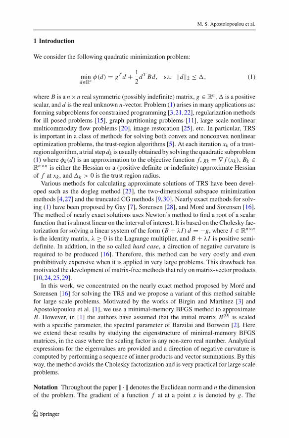
1 Introduction

We consider the following quadratic minimization problem:

mind∈Rn

φ(d) = gT d + 1

2dT Bd, s.t. ‖d‖2 ≤ �, (1)

where B is a n ×n real symmetric (possibly indefinite) matrix, g ∈ Rn,� is a positive

scalar, and d is the real unknown n-vector. Problem (1) arises in many applications as:forming subproblems for constrained programming [3,21,22], regularization methodsfor ill-posed problems [15], graph partitioning problems [11], large-scale nonlinearmulticommodity flow problems [20], image restoration [25], etc. In particular, TRSis important in a class of methods for solving both convex and nonconvex nonlinearoptimization problems, the trust-region algorithms [5]. At each iteration xk of a trust-region algorithm, a trial step dk is usually obtained by solving the quadratic subproblem(1) where φk(d) is an approximation to the objective function f, gk = ∇ f (xk), Bk ∈R

n×n is either the Hessian or a (positive definite or indefinite) approximate Hessianof f at xk , and �k > 0 is the trust region radius.

Various methods for calculating approximate solutions of TRS have been devel-oped such as the dogleg method [23], the two-dimensional subspace minimizationmethods [4,27] and the truncated CG methods [9,30]. Nearly exact methods for solv-ing (1) have been proposed by Gay [7], Sorensen [28], and Moré and Sorensen [16].The method of nearly exact solutions uses Newton’s method to find a root of a scalarfunction that is almost linear on the interval of interest. It is based on the Cholesky fac-torization for solving a linear system of the form (B + λI ) d = −g, where I ∈ R

n×n

is the identity matrix, λ ≥ 0 is the Lagrange multiplier, and B + λI is positive semi-definite. In addition, in the so called hard case, a direction of negative curvature isrequired to be produced [16]. Therefore, this method can be very costly and evenprohibitively expensive when it is applied in very large problems. This drawback hasmotivated the development of matrix-free methods that rely on matrix-vector products[10,24,25,29].

In this work, we concentrated on the nearly exact method proposed by Moré andSorensen [16] for solving the TRS and we propose a variant of this method suitablefor large scale problems. Motivated by the works of Birgin and Martínez [3] andApostolopoulou et al. [1], we use a minimal-memory BFGS method to approximateB. However, in [1] the authors have assumed that the initial matrix B(0) is scaledwith a specific parameter, the spectral parameter of Barzilai and Borwein [2]. Herewe extend these results by studying the eigenstructure of minimal-memory BFGSmatrices, in the case where the scaling factor is any non-zero real number. Analyticalexpressions for the eigenvalues are provided and a direction of negative curvature iscomputed by performing a sequence of inner products and vector summations. By thisway, the method avoids the Cholesky factorization and is very practical for large scaleproblems.

Notation Throughout the paper ‖ ·‖ denotes the Euclidean norm and n the dimensionof the problem. The gradient of a function f at at a point x is denoted by g. The

123


Moore–Penrose generalized inverse of a matrix A is denoted by A†. For a symmetricA ∈ R

n×n , assume that λ1 ≤ · · · ≤ λn are its eigenvalues sorted into non-decreasingorder. We indicate that a matrix is positive semi-definite (positive definite) by A ≥ 0(A > 0, respectively).

2 Properties of the minimal-memory BFGS matrices

In this section we study the eigenstructure of the matrix B in the quadratic model (1).The computation of B is based on the minimal memory BFGS method [14,17]. TheHessian approximation is updated using the BFGS formula

Bk+1 = Bk − BksksTk Bk

sTk Bksk

+ yk yTk

sTk yk

, (2)

where in the vector pair sk = xk+1 − xk and yk = gk+1 − gk is stored curvatureinformation from the most previous iteration. We consider as the initial matrix B(0),the diagonal matrix B(0) = θ I , where θ ∈ R \ {0} is a scaled parameter. Possiblechoices for the parameter θ could be: θk+1 = 1, which results the conjugate gradientmethod proposed by Shanno [26]; θk+1 = yT

k yk/sTk yk which constitutes the most

successful scaling factor [18, pp. 200]; or θk+1 = sTk yk/sT

k sk , the inverse of Barzilaiand Borwein’s [2] spectral parameter, which lies between the largest and the smallesteigenvalues of the average Hessian.

By setting B(0) = θk+1 I in (2), we obtain the minimal-memory BFGS update,defined as

Bk+1 = θk+1 I − θk+1sksT

k

sTk sk

+ yk yTk

sTk yk

. (3)

Note that in the quadratic model (1), the approximate Hessian matrix can be positivedefinite or indefinite. Hence, for the remaining of the paper we only assume that‖B‖ is bounded, that is, there is a positive constant M , such that ‖Bk‖ ≤ M < ∞,for all k.

Theorem 1 Suppose that one update is applied to the symmetric matrix B(0) =θ I, θ ∈ R \ {0}, using the vector pair {sk, yk} and the BFGS formula. The char-acteristic polynomial of the symmetric matrix Bk+1 ∈ R

n×n, defined in (3), has thegeneral form

p(λ) = (λ − θk+1)n−2 (λ2 − β1λ + β2), (4)

where β1 = θk+1 + (yT

k yk)/(sT

k yk), and β2 = θk+1

(sT

k yk)/(sT

k sk). Moreover, if

the vectors sk and yk are linearly independent then the smallest eigenvalue of Bk+1 isdistinct.

Proof First we show that Bk+1 has at most two distinct eigenvalues. To this end, weconsider the matrix B̄ = θk+1 I − θk+1sksT

k /sTk sk with rank (n − 1). Applying the

123


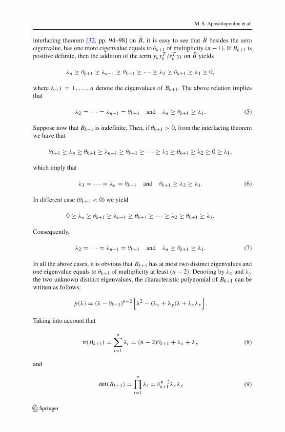
interlacing theorem [32, pp. 94–98] on B̄, it is easy to see that B̄ besides the zeroeigenvalue, has one more eigenvalue equals to θk+1 of multiplicity (n − 1). If Bk+1 ispositive definite, then the addition of the term yk yT

k /sTk yk on B̄ yields

λn ≥ θk+1 ≥ λn−1 ≥ θk+1 ≥ · · · ≥ λ2 ≥ θk+1 ≥ λ1 ≥ 0,

where λi , i = 1, . . . , n denote the eigenvalues of Bk+1. The above relation impliesthat

λ2 = · · · = λn−1 = θk+1 and λn ≥ θk+1 ≥ λ1. (5)

Suppose now that Bk+1 is indefinite. Then, if θk+1 > 0, from the interlacing theoremwe have that

θk+1 ≥ λn ≥ θk+1 ≥ λn−1 ≥ θk+1 ≥ · · · ≥ λ3 ≥ θk+1 ≥ λ2 ≥ 0 ≥ λ1,

which imply that

λ3 = · · · = λn = θk+1 and θk+1 ≥ λ2 ≥ λ1. (6)

In different case (θk+1 < 0) we yield

0 ≥ λn ≥ θk+1 ≥ λn−1 ≥ θk+1 ≥ · · · ≥ λ2 ≥ θk+1 ≥ λ1.

Consequently,

λ2 = · · · = λn−1 = θk+1 and λn ≥ θk+1 ≥ λ1. (7)

In all the above cases, it is obvious that Bk+1 has at most two distinct eigenvalues andone eigenvalue equals to θk+1 of multiplicity at least (n − 2). Denoting by λx and λy

the two unknown distinct eigenvalues, the characteristic polynomial of Bk+1 can bewritten as follows:

p(λ) = (λ − θk+1)n−2

[λ2 − (λx + λy)λ + λxλy

].

Taking into account that

tr(Bk+1) =n∑

i=1

λi = (n − 2)θk+1 + λx + λy (8)

and

det(Bk+1) =n∏

i=1

λi = θn−2k+1 λxλy (9)

123


we have that

p(λ) = (λ − θk+1)n−2

{λ2 − [

tr(Bk+1) − (n − 2)θk+1]λ + det(Bk+1)/θ

n−2k+1

}.

Using the well-known properties of the trace and determinant of matrices, we yield:

tr(Bk+1) = tr

(

θk+1 I − θk+1sksT

k

sTk sk

+ yk yTk

sTk yk

)

= (n − 1)θk+1 + yTk yk

sTk yk

, (10)

and

det(Bk+1) = det

(

θk+1 I − θk+1sksT

k

sTk sk

+ yk yTk

sTk yk

)

= det (θk+1 I ) det

(

I − sksTk

sTk sk

+ yk yTk

θk+1sTk yk

)

= θnk+1

[(

1 − sTk sk

sTk sk

) (

1 + yTk yk

θk+1sTk yk

)

+ sTk yk

θk+1sTk sk

]

= θn−1k+1

sTk yk

sTk sk

(11)

Hence,

β1 = tr(Bk+1) − (n − 2)θk+1 = θk+1 + (yTk yk)/(s

Tk yk),

β2 = det(Bk+1)/θn−2k+1 = θk+1(s

Tk yk)/(s

Tk sk),

and relation (4) follows immediately.It remains to show that when sk and yk are linearly independent, the smallest eigen-

value is distinct. Suppose that the vectors sk and yk are linearly independent and assumethat Bk+1 has at most one distinct eigenvalue, which implies that either λx = θk+1or λy = θk+1. Combining relation (8) with (10), and (9) with (11), we have that(sT

k yk)2 = sT

k sk yTk yk . Hence, the vectors sk and yk are collinear, which contradicts

the hypothesis. Thus, if the vectors are linearly independent, then Bk+1 has exactlytwo distinct eigenvalues. Combining relations (5), (6) and (7), easily we can concludethat λ1 is always distinct. �

Let us examine the case where the vectors sk and yk are collinear. Assuming thatyk = κsk, κ ∈ R, Bk+1 becomes

Bk+1 = θk+1 I + (κ − θk+1)sksT

k

sTk sk

. (12)

123


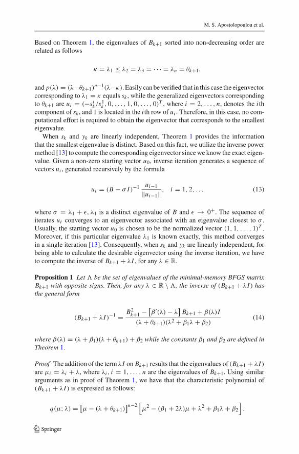
Based on Theorem 1, the eigenvalues of Bk+1 sorted into non-decreasing order arerelated as follows

κ = λ1 ≤ λ2 = λ3 = · · · = λn = θk+1,

and p(λ) = (λ−θk+1)n−1(λ−κ). Easily can be verified that in this case the eigenvector

corresponding to λ1 = κ equals sk , while the generalized eigenvectors correspondingto θk+1 are ui = (−si

k/s1k , 0, . . . , 1, 0, . . . , 0)T , where i = 2, . . . , n, denotes the i th

component of sk , and 1 is located in the i th row of ui . Therefore, in this case, no com-putational effort is required to obtain the eigenvector that corresponds to the smallesteigenvalue.

When sk and yk are linearly independent, Theorem 1 provides the informationthat the smallest eigenvalue is distinct. Based on this fact, we utilize the inverse powermethod [13] to compute the corresponding eigenvector since we know the exact eigen-value. Given a non-zero starting vector u0, inverse iteration generates a sequence ofvectors ui , generated recursively by the formula

ui = (B − σ I )−1 ui−1

‖ui−1‖ , i = 1, 2, . . . (13)

where σ = λ1 + ε, λ1 is a distinct eigenvalue of B and ε → 0+. The sequence ofiterates ui converges to an eigenvector associated with an eigenvalue closest to σ .Usually, the starting vector u0 is chosen to be the normalized vector (1, 1, . . . , 1)T .Moreover, if this particular eigenvalue λ1 is known exactly, this method convergesin a single iteration [13]. Consequently, when sk and yk are linearly independent, forbeing able to calculate the desirable eigenvector using the inverse iteration, we haveto compute the inverse of Bk+1 + λI , for any λ ∈ R.

Proposition 1 Let be the set of eigenvalues of the minimal-memory BFGS matrixBk+1 with opposite signs. Then, for any λ ∈ R \ , the inverse of (Bk+1 + λI ) hasthe general form

(Bk+1 + λI )−1 = B2k+1 − [

β ′(λ) − λ]

Bk+1 + β(λ)I

(λ + θk+1)(λ2 + β1λ + β2)(14)

where β(λ) = (λ + β1)(λ + θk+1) + β2 while the constants β1 and β2 are defined inTheorem 1.

Proof The addition of the term λI on Bk+1 results that the eigenvalues of (Bk+1 + λI )are μi = λi + λ, where λi , i = 1, . . . , n are the eigenvalues of Bk+1. Using similararguments as in proof of Theorem 1, we have that the characteristic polynomial of(Bk+1 + λI ) is expressed as follows:

q(μ; λ) = [μ − (λ + θk+1)

]n−2[μ2 − (β1 + 2λ)μ + λ2 + β1λ + β2

].

123


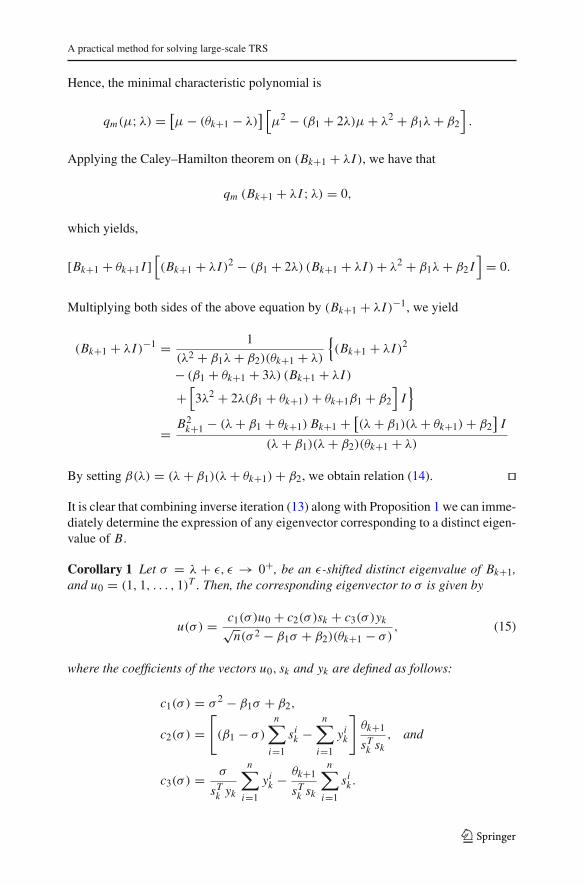
Hence, the minimal characteristic polynomial is

qm(μ; λ) = [μ − (θk+1 − λ)

] [μ2 − (β1 + 2λ)μ + λ2 + β1λ + β2

].

Applying the Caley–Hamilton theorem on (Bk+1 + λI ), we have that

qm (Bk+1 + λI ; λ) = 0,

which yields,

[Bk+1 + θk+1 I ][(Bk+1 + λI )2 − (β1 + 2λ) (Bk+1 + λI ) + λ2 + β1λ + β2 I

]= 0.

Multiplying both sides of the above equation by (Bk+1 + λI )−1, we yield

(Bk+1 + λI )−1 = 1

(λ2 + β1λ + β2)(θk+1 + λ)

{(Bk+1 + λI )2

− (β1 + θk+1 + 3λ) (Bk+1 + λI )

+[3λ2 + 2λ(β1 + θk+1) + θk+1β1 + β2

]I}

= B2k+1 − (λ + β1 + θk+1) Bk+1 + [

(λ + β1)(λ + θk+1) + β2]

I

(λ + β1)(λ + β2)(θk+1 + λ)

By setting β(λ) = (λ + β1)(λ + θk+1) + β2, we obtain relation (14). �

It is clear that combining inverse iteration (13) along with Proposition 1 we can imme-diately determine the expression of any eigenvector corresponding to a distinct eigen-value of B.

Corollary 1 Let σ = λ + ε, ε → 0+, be an ε-shifted distinct eigenvalue of Bk+1,and u0 = (1, 1, . . . , 1)T . Then, the corresponding eigenvector to σ is given by

u(σ ) = c1(σ )u0 + c2(σ )sk + c3(σ )yk√n(σ 2 − β1σ + β2)(θk+1 − σ)

, (15)

where the coefficients of the vectors u0, sk and yk are defined as follows:

c1(σ ) = σ 2 − β1σ + β2,

c2(σ ) =[

(β1 − σ)

n∑

i=1

sik −

n∑

i=1

yik

]θk+1

sTk sk

, and

c3(σ ) = σ

sTk yk

n∑

i=1

yik − θk+1

sTk sk

n∑

i=1

sik .

123


Proof From Proposition 1, by setting λ = −σ in (14) we obtain the expression of(B − σ I )−1. Therefore, the application of inverse iteration (13) yields

u(σ ) = (B − σ I )−1 u0

‖u0‖ = B2k+1u0 − [

β ′(−σ) + σ]

Bk+1u0 + β(−σ)u0

(−σ + θk+1)(σ 2 − β1σ + β2)‖u0‖ . (16)

The vectors Bk+1u0 and B2k+1u0 can be obtained by the iterative form

Bk+1wi = θk+1wi − θk+1sT

k wi

sTk sk

sk + yTk wi

sTk yk

yk i = 0, 1, (17)

with w0 = u0. Using relation (17) and the fact that ‖u0‖ = √n, after some algebraic

computations, relation (16) is reduced to (15). �

3 Solving the TRS using the minimal-memory BFGS method

In this section we apply the results of Sect. 2 for solving the large scale TRS. Aglobal solution to the TRS (1) is characterized by the following well known theorem[7,28,16]:

Theorem 2 A feasible vector d∗ is a solution to (1) with corresponding Lagrangemultiplier λ∗ if and only if d∗, λ∗ satisfy (B + λ∗ I ) d∗ = −g, where B + λ∗ I ispositive semi-definite, λ∗ ≥ 0, and λ∗(� − ‖d∗‖) = 0.

From the above Theorem we can distinguish two cases, the standard and the hardcase. In the standard case, the solution of the TRS can be summarized as follows:

1. If λ1 > 0 (the matrix is positive definite), thena. if ‖B−1g‖ ≤ �, then λ∗ = 0 and d∗ = B−1g.b. if ‖B−1g‖ > �, then for the unique λ∗ ∈ (0,∞) such that ‖ (B + λ∗ I )−1

g‖=�, d∗ = − (B + λ∗ I )−1 g.2. If λ1 ≤ 0 (the matrix is indefinite), then if ‖B−1g‖ > �, for the unique λ∗ ∈

(−λ1,∞) such that ‖ (B + λ∗ I )−1 g‖ = �, d∗ = − (B + λ∗ I )−1 g.

As we can observe, the optimal non-negative Lagrange multiplier λ∗ belongs to theopen interval (−λ1,∞). When λ∗ �= 0, the TRS (1) has a boundary solution, i.e.,‖d∗‖ = �. In this case, the given n-dimensional constrained optimization problem isreduced into a zero-finding problem in a single scalar variable λ, namely, ‖d(λ)‖−� =0, where the trial step d(λ) is a solution of the linear system (B + λI ) d = −g. Moréand Sorensen [16] have proved that it is more convenient to solve the equivalentequation (secular equation) φ(λ) ≡ 1/� − 1/‖d(λ)‖ = 0, that exploits the rationalstructure of ‖d(λ)‖2. The solution λ of the secular equation is based on Newton’smethod,

λ�+1 = λ� + ‖d(λ)‖‖d(λ)‖′

(� − ‖d(λ)‖

�

), � = 0, 1, 2, . . . . (18)

123


In Newton’s iteration (18) a safeguarding is required to ensure that a solution is found.The safeguarding depends on the fact that φ is convex and strictly decreasing in(−λ1,∞). It ensures that −λ1 ≤ λ�, and therefore B + λ� I is always semi-positivedefinite [16].

The hard case occurs when B is indefinite and g is orthogonal to every eigenvectorcorresponding to the most negative eigenvalue λ1 of the matrix. In this case, there isno λ ∈ (−λ1,∞) such that ‖ (B + λI )−1 g‖ = �. The optimal Lagrange multiplieris λ∗ = −λ1, the matrix (B − λ1 I ) is singular, and a direction of negative curvaturemust be calculated in order to ensure that ‖d‖ = �. Consequently, in the hard case,the optimal solution to the TRS is d∗ = − (B − λ1 I )† g + τu, where τ ∈ R is suchthat ‖− (B − λ1 I )† g + τu‖ = � and u is a normalized eigenvector corresponding toλ1. Moré and Sorensen [16] have showed that the choice of τ that ensures ‖d‖ = �,is

τ = �2 − ‖p‖2

pT u1 + sgn(pT u)√

(pT u)2 + �2 − ‖p‖2, (19)

where p = − (B − λ1 I )† g.The above analysis indicates that for been able to solve the TRS (1), we should

compute the smallest eigenvalue λ1 of B, the inverse of B +λI for computing the trialstep d(λ), and, in the hard case, the unit eigenvector u corresponding to λ1. Moreover,the definition of a simple safeguarding scheme in Newton’s iteration (18) requires alsothe largest eigenvalue λn .

In Sect. 2, we have studied all these aspects in detail. The Algorithm 1 (see [1]),handles both the standard and the hard case and computes a nearly exact solution of thesubproblem (1) without using the Cholesky factorization. Moreover, the knowledgeof the extreme eigenvalues, results in a straightforward safeguarding procedure for λ.

Algorithm 1 (Computation of the trial step)

Step 1: Compute the eigenvalues λi of B; given ε → 0+, set the bounds λL :=max(0,−λ1 + ε) and λU := max |λi | + (1 + ε)‖g‖/�.

Step 2: If λ1 > 0, then initialize λ by setting λ := 0 and compute d(λ); if ‖d‖ ≤ �

stop; else go to Step 4.Step 3: Initialize λ by setting λ := −λ1 + ε such that B + λI is positive definite and

compute d(λ);a. if ‖d‖ > � go to Step 4;b. if ‖d‖ = � stop;c. if ‖d‖ < � compute τ and u1 such that ‖− (B + λI )−1 g + τu1‖ = �;

set d := d + τu1 and stop;Step 4: Use Newton’s method to find λ ∈ [λL , λU ] and compute d(λ);Step 5: If ‖d‖ = � stop; else update λL and λU such that λL ≤ λ ≤ λU and go to

Step 4.

In Step 1 of Algorithm 1 the eigenvalues are computed by solving the character-istic equation p(λ) = 0, defined in relation (4). Obviously, the two possibly distinct

123


eigenvalues are

(−β1 ±

√β2

1 − 4β2

)/2 while the eigenvalue θk+1 is multiple. The

safeguarding scheme required for Newton’s iteration (18) uses the parameters λL andλU such that [λL , λU ] is an interval of uncertainty which contains the optimal λ∗. Theinitial bounds λL and λU have been proposed by Nocedal and Yuan [19]. Clearly, thelower bound λL is greater than −λ1, which ensures that B + λI is always positivedefinite.

Note that in Steps 2, 3 and 4, the trial step d(λ) is computed by solving the linearsystem (B + λI ) d(λ) = −g. Using Proposition 1, along with relations (17), the trialstep is computed immediately by the expression

d(λ) = −cg(λ)g + cs(λ)sk + cy(λ)yk

(λ2 + β1λ + β2)(λ + θk+1), (20)

where the coefficients are defined as follows

cg(λ) = λ2 + β1λ + β2,

cs(λ) =[(λ + β1) sT

k gk+1 − yTk gk+1

] θk+1

sTk sk

, and

cy(λ) = − yTk gk+1

sTk yk

λ − sTk gk+1

sTk sk

θk+1.

In Step 3(c), scalar τ is computed by Eq. (19), while for the computation of theeigenvector u1 corresponding to λ1, we take into account the relation between thevectors sk and yk . If the vectors sk and yk are linearly independent, then u1 = u/‖u‖,where u is computed by means of relation (15) in Corolarry 1. In different case, u1equals to the normalized vector sk , as explained in Sect. 2.

In Steps 4 and 5, Newton’s iteration (18) is utilized for computing the Lagrangemultiplier λ. In (18), we have that

‖d(λ)‖′ = −d(λ)T (B + λI )−1 d(λ)/‖d(λ)‖,

and thus, the iterative scheme becomes

λ�+1 = λ� + ‖d(λ)‖2

d(λ)T (Bk+1 + λI )−1 d(λ)

(‖d(λ)‖ − �

�

), � = 0, 1, . . . (21)

Denoting by = d(λ)T (Bk+1 + λI )−1 d(λ) the denominator in (21), and taking intoaccount that Bk+1 d(λ) = − [

λ d(λ) + gk+1]

holds, then by Proposition 1 we obtainthat

=[β(λ) + λβ ′(λ)

] ‖d(λ)‖2 + [β ′(λ) + λ

]d(λ)T gk+1 + ‖gk+1‖2

(λ + θk+1)(λ2 + β1λ + β2). (22)

123


If sk and yk are collinear and relation yk = κsk holds, then relations (20) and (22) arereduced to

d(λ) = − 1

(λ + θk+1)gk+1 + (κ − θk+1)sT

k gk+1

(λ + κ)(λ + θk+1)sTk sk

sk,

and

= (2λ + β1)‖d(λ)‖2 + d(λ)T gk+1

λ2 + β1λ + β2,

respectively.

4 Numerical experiments and analysis

For illustrating the behavior of the proposed method in both the standard and thehard case, we use randomly generated TRS instances with dimensions from 100 up to15,000,000 variables. The experiments are consisted by medium-size problems withdimensions n = 100, 500, 1,000, by larger-size problems (n = 104, 105, 106), andby very large problems (n = 2 × 106, 3 × 106, . . . , 15 × 106).

For each dimension n, 1,000 random instances of the TRS (1) were generated asfollows. The coordinates of the vectors g, s, and y were chosen independently fromuniform distributions in the interval (−102,+102). For the numerical testing we imple-mented Algorithm 1 as MBFGS1, using FORTRAN 90 and all numerical experimentswere performed on a Pentium 1.86 GHz personal computer with 2GB of RAM runningLinux operating system.

We compared our method with the GQTPAR, and the GLTR algorithm. The GQT-PAR algorithm is available as subroutine dgqt in the MINPACK-2 package,2 andis based on the ideas described in Moré and Sorensen [16] for computing a nearlyexact solution of (1). The method uses the Cholesky factorization for calculating therequired derivatives during the computation of the Newton step for λ, as well as for thesafeguarding and updating of the Lagrange multiplier. The GLTR algorithm proposedby Gould et al. [9], is available as the FORTRAN 90 module HSL_VF053 in theHarwell Subroutine Library [12]. This method is based on a Lanczos tridiagonaliza-tion of the matrix B and on the solution of a sequence of problems restricted to Krylovsubspaces of R

n . It is an alternative to the Steihaug–Toint algorithm [30,31] and itcomputes an approximate solution of (1). The algorithm requires only matrix–vectormultiplications while it exploits the sparsity of B.

Note that the same set of random instances was used for each algorithm. We considerthat a TRS instance was successfully solved, if a solution satisfying ‖(B + λI ) d − g‖≤ 10−3 was computed for both the standard and the hard case. The maximum num-ber of Newton’s iterations allowed was 200 and the trust region radius was fixed as

1 Available from http://www.math.upatras.gr/~msa/2 Available from ftp://info.mcs.anl.gov/pub/MINPACK-2/gqt/3 Available from http://www.hsl.rl.ac.uk

123

http://www.math.upatras.gr/~msa/

ftp://info.mcs.anl.gov/pub/MINPACK-2/gqt/

http://www.hsl.rl.ac.uk


� = 10. For dimensions larger than 1,000, results are reported only for MBFGS andGLTR algorithms, due to the storage requirements of GQTPAR for factoring B. More-over, the GLTR algorithm is not reported in the comparison results for the hard case,since it computes an approximate solution and not a nearly exact solution of the TRS.

For each dimension, a table summarizing the performance of all algorithms forsimulations that reached solution is presented. The reported metrics are Newton’siterations (i t) and solution accuracy (acc). The descriptives statistics over 1,000 exper-iments are: the mean and standard deviation, as well as the minimum and maximumvalues. To show both the efficacy and accuracy of our method, we have used the per-formance profile proposed by Dolan and Moré [6]. The performance profile plots thefraction of problems for which any given method is within a factor of the best solver.The left axis of the plot shows the percentage of the problems for which a method isthe fastest (efficiency). The right side of the plot gives the percentage of the problemsthat were successfully solved by each of the methods (robustness). The reported per-formance profiles have been created using the Libopt4 environment [8], an excellentset of tools written in Perl.

4.1 Random experiments in the standard case

Firstly, we present the behavior of the proposed method in the standard case. For eachdimension between n = 100 and n = 106, we have considered the following cases:

(a) sk, yk are linearly independent and θk+1 = 1;(b) sk, yk are linearly independent and θk+1 = (yT

k yk)/(sTk yk);

(c) sk, yk are collinear and θk+1 = 1;(d) sk, yk are collinear and θk+1 = (yT

k yk)/(sTk yk).

If θk+1 = 1, then the initial matrix B(0) is the identity matrix. In different case, thescalar parameter θ is chosen to be the one proposed in the literature [18] for scalingthe initial matrix in the BFGS method. The above cases were considered for analyzingthe behavior of the proposed method in all cases concerning the vector pair {s, y},as well as the scaling factor. As a total, we have 12,000 medium size experiments(n = 100, 500, and 1,000) and 12,000 large size experiments (n = 104, 105, and106).

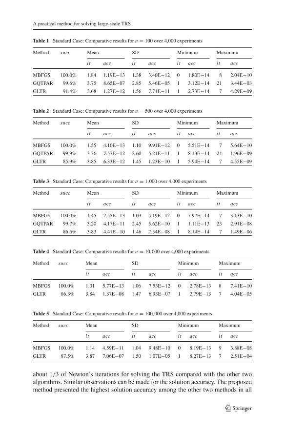
Tables 1, 2, 3, 4, 5 and 6 summarize the results for the experiments with dimensionsfrom n = 100 up to n = 106. In all tables, the first column denotes the method, whilethe second column reports the percentage of the successfully (succ) solved instanceswithin the required accuracy (10−3). In Tables 4, 5 and 6 the GQTPAR method wasomitted from the comparisons due to memory limitations.

The results in all tables show that the MBFGS algorithm has solved all problemssuccessfully, in all dimensions, in contrast with the other two algorithms that failedto solve all experiments within the required accuracy. Moreover, MBFGS outperformsboth GQTPAR and GLTR algorithms in terms of Newton’s iterations, since in all sta-tistical metrics it exhibited the lowest value. Actually, on average the MBFGS required

4 Available from http://www-rocq.inria.fr/~gilbert/modulopt/libopt/

123

http://www-rocq.inria.fr/~gilbert/modulopt/libopt/


Table 1 Standard Case: Comparative results for n = 100 over 4,000 experiments

Method succ Mean SD Minimum Maximum

i t acc i t acc i t acc i t acc

MBFGS 100.0% 1.84 1.19E−13 1.38 3.40E−12 0 1.80E−14 8 2.04E−10

GQTPAR 99.6% 3.75 8.65E−07 2.85 5.46E−05 1 3.12E−14 21 3.44E−03

GLTR 91.4% 3.68 1.27E−12 1.56 7.71E−11 1 2.73E−14 7 4.29E−09

Table 2 Standard Case: Comparative results for n = 500 over 4,000 experiments



MBFGS 100.0% 1.55 4.10E−13 1.10 9.91E−12 0 5.51E−14 7 5.64E−10

GQTPAR 99.9% 3.36 7.57E−12 2.60 5.21E−11 1 8.13E−14 24 1.96E−09

GLTR 85.9% 3.85 6.33E−12 1.45 1.23E−10 1 5.94E−14 7 4.55E−09

Table 3 Standard Case: Comparative results for n = 1,000 over 4,000 experiments



MBFGS 100.0% 1.45 2.55E−13 1.03 5.19E−12 0 7.97E−14 7 3.13E−10

GQTPAR 99.7% 3.20 4.17E−11 2.45 5.62E−10 1 1.11E−13 23 2.91E−08

GLTR 86.5% 3.83 4.41E−10 1.46 2.54E−08 1 8.14E−14 7 1.49E−06




MBFGS 100.0% 1.31 5.77E−13 1.06 7.53E−12 0 2.78E−13 8 7.41E−10

GLTR 86.3% 3.84 1.37E−08 1.47 6.93E−07 1 2.79E−13 7 4.04E−05




MBFGS 100.0% 1.14 4.59E−11 1.04 9.48E−10 0 8.19E−13 9 3.88E−08

GLTR 87.5% 3.87 7.06E−07 1.50 1.07E−05 1 8.27E−13 7 2.51E−04

about 1/3 of Newton’s iterations for solving the TRS compared with the other twoalgorithms. Similar observations can be made for the solution accuracy. The proposedmethod presented the highest solution accuracy among the other two methods in all

123


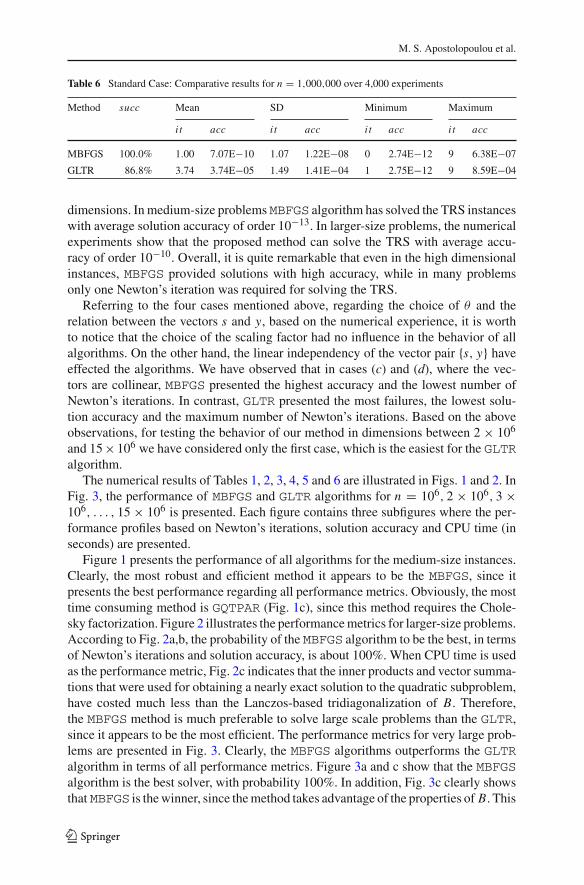
Table 6 Standard Case: Comparative results for n = 1,000,000 over 4,000 experiments



MBFGS 100.0% 1.00 7.07E−10 1.07 1.22E−08 0 2.74E−12 9 6.38E−07

GLTR 86.8% 3.74 3.74E−05 1.49 1.41E−04 1 2.75E−12 9 8.59E−04

dimensions. In medium-size problems MBFGS algorithm has solved the TRS instanceswith average solution accuracy of order 10−13. In larger-size problems, the numericalexperiments show that the proposed method can solve the TRS with average accu-racy of order 10−10. Overall, it is quite remarkable that even in the high dimensionalinstances, MBFGS provided solutions with high accuracy, while in many problemsonly one Newton’s iteration was required for solving the TRS.

Referring to the four cases mentioned above, regarding the choice of θ and therelation between the vectors s and y, based on the numerical experience, it is worthto notice that the choice of the scaling factor had no influence in the behavior of allalgorithms. On the other hand, the linear independency of the vector pair {s, y} haveeffected the algorithms. We have observed that in cases (c) and (d), where the vec-tors are collinear, MBFGS presented the highest accuracy and the lowest number ofNewton’s iterations. In contrast, GLTR presented the most failures, the lowest solu-tion accuracy and the maximum number of Newton’s iterations. Based on the aboveobservations, for testing the behavior of our method in dimensions between 2 × 106

and 15 × 106 we have considered only the first case, which is the easiest for the GLTRalgorithm.

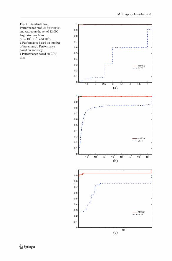
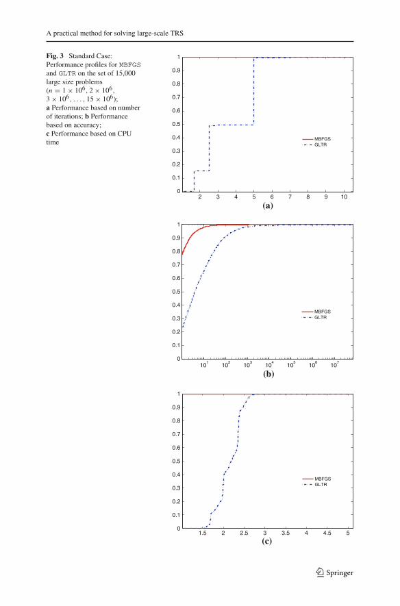
The numerical results of Tables 1, 2, 3, 4, 5 and 6 are illustrated in Figs. 1 and 2. InFig. 3, the performance of MBFGS and GLTR algorithms for n = 106, 2 × 106, 3 ×106, . . . , 15 × 106 is presented. Each figure contains three subfigures where the per-formance profiles based on Newton’s iterations, solution accuracy and CPU time (inseconds) are presented.

Figure 1 presents the performance of all algorithms for the medium-size instances.Clearly, the most robust and efficient method it appears to be the MBFGS, since itpresents the best performance regarding all performance metrics. Obviously, the mosttime consuming method is GQTPAR (Fig. 1c), since this method requires the Chole-sky factorization. Figure 2 illustrates the performance metrics for larger-size problems.According to Fig. 2a,b, the probability of the MBFGS algorithm to be the best, in termsof Newton’s iterations and solution accuracy, is about 100%. When CPU time is usedas the performance metric, Fig. 2c indicates that the inner products and vector summa-tions that were used for obtaining a nearly exact solution to the quadratic subproblem,have costed much less than the Lanczos-based tridiagonalization of B. Therefore,the MBFGS method is much preferable to solve large scale problems than the GLTR,since it appears to be the most efficient. The performance metrics for very large prob-lems are presented in Fig. 3. Clearly, the MBFGS algorithms outperforms the GLTRalgorithm in terms of all performance metrics. Figure 3a and c show that the MBFGSalgorithm is the best solver, with probability 100%. In addition, Fig. 3c clearly showsthat MBFGS is the winner, since the method takes advantage of the properties of B. This

123


Fig. 1 Standard Case:Performance profiles forMBFGS, GQTPAR and GLTR onthe set of 12,000 medium sizeproblems (n = 100, 500, and1,000). a Performance based onnumber of iterations;b Performance based onaccuracy; c Performance basedon CPU time

2 3 4 5 6 7 8 90

0.1

0.2

0.3

0.4

0.5

0.6

0.7

0.8

0.9

1

MBFGSGQTPARGLTR

102

104

106

108

10100

0.1

0.2

0.3

0.4

0.5

0.6

0.7

0.8

0.9

1

MBFGSGQTPARGLTR

101

102

103

1040

0.1

0.2

0.3

0.4

0.5

0.6

0.7

0.8

0.9

1

MBFGSGQTPARGLTR

(a)

(b)

(c)

123


Fig. 2 Standard Case:Performance profiles for MBFGSand GLTR on the set of 12,000large size problems(n = 104, 105, and 106).a Performance based on numberof iterations; b Performancebased on accuracy;c Performance based on CPUtime

1.5 2 2.5 3 3.5 4 4.5 50

0.1

0.2

0.3

0.4

0.5

0.6

0.7

0.8

0.9

1

MBFGSGLTR

101

102

103

104

105

106

107

108

0

0.1

0.2

0.3

0.4

0.5

0.6

0.7

0.8

0.9

1

MBFGSGLTR

1010

0.1

0.2

0.3

0.4

0.5

0.6

0.7

0.8

0.9

1

MBFGSGLTR

(a)

(b)

(c)

123


Fig. 3 Standard Case:Performance profiles for MBFGSand GLTR on the set of 15,000large size problems(n = 1 × 106, 2 × 106,

3 × 106, . . . , 15 × 106);a Performance based on numberof iterations; b Performancebased on accuracy;c Performance based on CPUtime

2 3 4 5 6 7 8 9 100

0.1

0.2

0.3

0.4

0.5

0.6

0.7

0.8

0.9

1

MBFGSGLTR

101

102

103

104

105

106

107

0

0.1

0.2

0.3

0.4

0.5

0.6

0.7

0.8

0.9

1

MBFGSGLTR

1.5 2 2.5 3 3.5 4 4.5 50

0.1

0.2

0.3

0.4

0.5

0.6

0.7

0.8

0.9

1

MBFGSGLTR

(a)

(b)

(c)

123


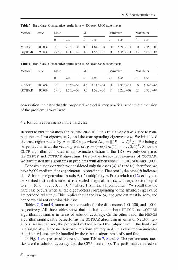
Table 7 Hard Case: Comparative results for n = 100 over 3,000 experiments



MBFGS 100.0% 0 9.13E−06 0.0 1.84E−04 0 8.24E−11 0 7.15E−03

GQTPAR 96.8% 27.52 1.41E−06 3.3 1.56E−05 18 6.45E−14 43 6.88E−04

Table 8 Hard Case: Comparative results for n = 500 over 3,000 experiments



MBFGS 100.0% 0 9.13E−06 0.0 2.11E−04 0 9.31E−11 0 7.94E−03

GQTPAR 96.0% 29.10 1.25E−06 3.7 1.58E−05 17 1.22E−08 52 7.97E−04

observation indicates that the proposed method is very practical when the dimensionof the problem is very large.

4.2 Random experiments in the hard case

In order to create instances for the hard case, Matlab’s routine eigswas used to com-pute the smallest eigenvalue λ1 and the corresponding eigenvector u. We initializedthe trust-region radius by � = 10.0�hc, where �hc = ‖ (B − λ1 I )† g‖. For being gperpendicular to u, the vector g was set g = (−u(n)/u(1), 0, . . . , 0, 1)T . Since theGLTR algorithm computes an approximate solution to the TRS, we only comparedthe MBFGS and GQTPAR algorithms. Due to the storage requirements of GQTPAR,we have tested the algorithms in problems with dimensions n = 100, 500, and 1,000.

For each dimension we have considered only the cases (a), (b) and (c), therefore, wehave 9,000 medium-size experiments. According to Theorem 1, the case (d) indicatesthat B has one eigenvalues equals θ , of multiplicity n. From relation (12) easily canbe verified that in this case, B is a scaled diagonal matrix, with eigenvectors equalto ei = (0, 0, . . . , 1, 0, . . . , 0)T , where 1 is in the i th component. We recall that thehard case occurs when all the eigenvectors corresponding to the smallest eigenvalueare perpendicular to g. This implies that in the case (d), the gradient must be zero, andhence we did not examine this case.

Tables 7, 8 and 9, summarize the results for the dimensions 100, 500, and 1,000,respectively. All three tables show that the behavior of both MBFGS and GQTPARalgorithms is similar in terms of solution accuracy. On the other hand, the MBFGSalgorithm significantly outperforms the GQTPAR algorithm in terms of Newton iter-ations. As we can see, the proposed method solved the subproblem in the hard casein a single step, since no Newton’s iterations are required. This observation indicatesthat the hard case can be handled by the MBFGS algorithm easily and fast.

In Fig. 4 are presented the results from Tables 7, 8 and 9. The performance met-rics are the solution accuracy and the CPU time (in s). The performance based on

123


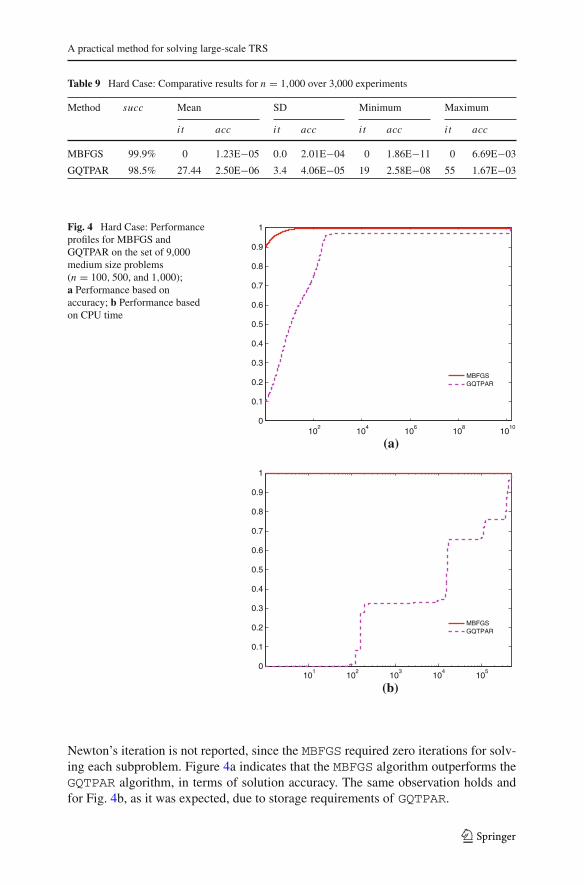
Table 9 Hard Case: Comparative results for n = 1,000 over 3,000 experiments



MBFGS 99.9% 0 1.23E−05 0.0 2.01E−04 0 1.86E−11 0 6.69E−03

GQTPAR 98.5% 27.44 2.50E−06 3.4 4.06E−05 19 2.58E−08 55 1.67E−03

Fig. 4 Hard Case: Performanceprofiles for MBFGS andGQTPAR on the set of 9,000medium size problems(n = 100, 500, and 1,000);a Performance based onaccuracy; b Performance basedon CPU time

102

104

106

108

1010

0

0.1

0.2

0.3

0.4

0.5

0.6

0.7

0.8

0.9

1

MBFGSGQTPAR

101

102

103

104

105

0

0.1

0.2

0.3

0.4

0.5

0.6

0.7

0.8

0.9

1

MBFGSGQTPAR

(a)

(b)

Newton’s iteration is not reported, since the MBFGS required zero iterations for solv-ing each subproblem. Figure 4a indicates that the MBFGS algorithm outperforms theGQTPAR algorithm, in terms of solution accuracy. The same observation holds andfor Fig. 4b, as it was expected, due to storage requirements of GQTPAR.

123


5 Conclusions

We have studied the eigenstructure of the minimal memory BFGS matrices in thegeneral case where the initial matrix is a scaled identity matrix. Our theoretical resultshave been applied for the solution of the trust region subproblem. Based on the fact thatthe algorithm uses only inner products and vector summations, the proposed methodis suitable and practical for solving large scale TRS. Our numerical experiments haveshown that the proposed method can easily handle both the standard and the hard case.It provides relatively fast solutions with high accuracy and small number of iterations.Moreover, it turns out that the hard case is the “easy” case for the proposed method.

References

1. Apostolopoulou, M.S., Sotiropoulos, D.G., Pintelas, P.: Solving the quadratic trust-region subproblemin a low-memory BFGS framework. Optim. Methods Softw. 23(5), 651–674 (2008)

2. Barzilai, J., Borwein, J.M.: Two point step size gradient method. IMA J. Numer. Anal. 8, 141–148(1988)

3. Birgin, E.G., Martínez, J.M.: Structured minimal-memory inexact quasi-Newton method and secantpreconditioners for augmented Lagrangian optimization. Comput. Optim. Appl. 39(1), 1–16 (2008)

4. Byrd, R.H., Schnabel, R.B., Shuldz, G.A.: Approximate solution of the trust region problem by mini-mization over two-dimensional subspaces. Math. Program. 40, 247–263 (1988)

5. Conn, A.R., Gould, N.I.M., Toint, Ph.L.: Trust-Region Methods. SIAM, Philadelphia, PA, USA (2000)6. Dolan, E., Moré, J.J.: Benchmarking optimization software with performance profiles. Math. Pro-

gram. 91, 201–213 (2002)7. Gay, D.M.: Computing optimal locally constrained steps. SIAM J. Sci. Stat. Comput. 2(2), 186–197

(1981)8. Gilbert, J.C., Jonsson, X.: LIBOPT—an environment for testing solvers on heterogeneous collections

of problems. The manual, version 2.1. INRIA Technical Report, RT-331 revised (2009)9. Gould, N.I.M., Lucidi, S., Roma, M., Toint, Ph.L.: Solving the trust-region subproblem using the

Lanczos method. SIAM J. Optim. 9(2), 504–525 (1999)10. Hager, W.W.: Minimizing a quadratic over a sphere. SIAM J. Optim. 12(1), 188–208 (2001)11. Hager, W.W., Krylyuk, Y.: Graph partitioning and continuous quadratic programming. SIAM J. Discret.

Math. 12(4), 500–523 (1999)12. HSL 2007: A collection of Fortran codes for large scale scientific computation (2007). Available from:

http://www.hsl.rl.ac.uk13. Ipsen, I.C.F.: Computing an eigenvector with inverse iteration. SIAM Rev. 39(2), 254–291 (1997)14. Liu, D.C., Nocedal, J.: On the limited memory BFGS method for large scale optimization. Math.

Program. 45(3), 503–528 (1989)15. Menke, W.: Geophysical Data Analysis: Discrete Inverse Theory. Academic Press, San Diego (1989)16. Moré, J.J., Sorensen, D.C.: Computing a trust region step. SIAM J. Sci. Stat. Comput. 4(3),

553–572 (1983)17. Nocedal, J.: Updating quasi-Newton matrices with limited storage. Math. Comput. 35(151),

773–782 (1980)18. Nocedal, J., Wright, S.J.: Numerical Optimization. Springer, New York (1999)19. Nocedal, J., Yuan, Y. : Combining trust region and line search techniques. In: Yuan, Y. (ed.) Advances

in Nonlinear Programming, pp. 153–175. Kluwer, Dordrecht (1998)20. Ouorou, A.: Implementing a proximal algorithm for some nonlinear multicommodity flow prob-

lems. Networks 49(1), 18–27 (2007)21. Pardalos, P.M., Resende, M. (eds.): Handbook of Applied Optimization. Oxford University

Press, Oxford (2002)22. Pardalos, P.M., Resende, M.: Interior point methods for global optimization. In: Terlaky, T. (ed.) Interior

Point Methods of Mathematical Programming, volume 5 of Applied Optimization, chapter 12, pp. 467–500. Kluwer, Dordrecht (1996)

123

http://www.hsl.rl.ac.uk


23. Powell, M.J.D.: A new algorithm for unconstrained optimization. In: Rosen, J.B., Mangasarian, O.L.,Ritter, K. (eds.) Nonlinear Programming, pp. 31–65. Academic Press, New York (1970)

24. Rendl, F., Wolkowicz, H.: A semidefinite framework for trust region subproblems with applicationsto large scale minimization. Math. Program. 77(2), 273–299 (1997)

25. Rojas, M., Santos, S.A., Sorensen, D.C.: A new matrix-free algorithm for the large-scale trust-regionsubproblem. SIAM J. Optim. 11(3), 611–646 (2000)

26. Shanno, D.F.: Conjugate gradient methods with inexact searches. Math. Oper. Res. 3(3), 244–256 (1978)

27. Shuldz, G.A., Schnabel, R.B., Byrd, R.H.: A family of trust-region-based algorithms for unconstrainedminimization with strong global convergence properties. SIAM J. Numer. Anal. 22(1), 47–67 (1985)

28. Sorensen, D.C.: Newton’s method with a model trust region modification. SIAM J. Numer.Anal. 19(2), 409–426 (1982)

29. Sorensen, D.C.: Minimization of a large-scale quadratic function subject to a spherical constraint. SIAMJ. Optim. 7(1), 141–161 (1997)

30. Steihaug, T.: The conjugate gradient method and trust regions in large scale optimization. SIAM J.Numer. Anal. 20(3), 626–637 (1983)

31. Toint, Ph.L.: Towards an efficient sparsity exploiting newton method for minimization. In: Duff,I.S. (ed.) Sparse Matrices and Their Uses, pp. 57–87. Academic Press, New York (1981)

32. Wilkinson, J.H.: The algebraic eigenvalue problem. Oxford University Press, London (1965)

123

a practical method for solving large-scale trs · e-mail: [email protected] 123. ... a practical...

Documents