a probabilistic analysis for transmission line structures
TRANSCRIPT

Retrospective Theses and Dissertations Iowa State University Capstones, Theses andDissertations
1993
A probabilistic analysis for transmission linestructuresKristine Marie SandageIowa State University
Follow this and additional works at: https://lib.dr.iastate.edu/rtd
Part of the Civil Engineering Commons, and the Structural Engineering Commons
This Thesis is brought to you for free and open access by the Iowa State University Capstones, Theses and Dissertations at Iowa State University DigitalRepository. It has been accepted for inclusion in Retrospective Theses and Dissertations by an authorized administrator of Iowa State University DigitalRepository. For more information, please contact [email protected].
Recommended CitationSandage, Kristine Marie, "A probabilistic analysis for transmission line structures" (1993). Retrospective Theses and Dissertations. 17265.https://lib.dr.iastate.edu/rtd/17265

A probabilistic analysis
for transmission line structures
by
Kristine Marie Sandage
A Thesis Submitted to the
Graduate Faculty in Partial Fulfillment of the
Requirements for the Degree of
MASTER OF SCIENCE
Department: Civil and Construction Engineering Major: Civil Engineering (Structural Engineering)
Approved:
Iowa State University Ames, Iowa
1993
Signatures redacted for privacy.
ii
TABLE OF CONTENTS
1. INTRODUCTION
1.1 History of Recent Failures
1. 2 Objectives
1.3 Organization of the study
2. LITERATURE REVIEW AND BACKGROUND
2.1 Transmission Line Structural Loading
2.2 Design Methodologies
2.3 Reliability Background
2.3.1 Limit state functions 2.3.2 Levels of analysis
2.3.2.1 2.3.2.2 2.3.2.3
Level 3: reliability analysis Level 2: reliability analysis Level 1: reliability analysis
Page
1
1
5
5
7
7
8
10
10 12
12 14 15
2.3.3 Reliability analyses of transmission structures
line
2.3.3.1
2.3.3.2 2.3.3.3 2.3.3.4 2.3.3.5
Reliability relationship between and structure Monte Carlo example Finite element example Plastic collapse failure example Newfoundland transmission line failure
3. DESCRIPTION OF THE PROCEDURE
3.1 Development of the Failure Functions
3.1.1 Generation of data points 3.1.2 Regression analysis
3.2 Reliability Analysis: First Order-Second Moment
15
line 15 17 18 20
22
26
26
27 28
Method 28
3.2.1 Reliability index 29
iii
3.2.2 Calculation of reliability index: Lind-Hasofer Method 30
3.3 Multiple Failure Functions
3.4 Example Problems
3.4.1 Ten-bar truss 3.4.2 Portal frame
4. ANALYSIS OF A TYPICAL TRANSMISSION LINE
34
36
36 47
56
4.1 Finite Element Model 56
4.2 Modelling Assumptions of the Transmission Line System 57
4.2.1 Geometry 4.2.2 Loads
4.3 Development of the Fragility Curve
4.3.1 4.3.2 4.3.3 4.3.4
Results of model 1 analysis Buckling failure Insulator failure Plastic mechanism failure
57 66
68
68 70 71 72
4.3.4.1 Plastic mechanism of cross arm 72 4.3.4.2 Plastic collapse of pole 74
4.3.5 Combination of failure modes 4.3.6 Interpretation of fragility curves
5. SUMMARY AND CONCLUSIONS
5.1 Summary
5. 2 Conclusions
5.3 Recommendations for Further Research
REFERENCES
ACKNOWLEDGMENTS
79 85
88
88
90
90
92
95
iv
LIST OF FIGURES
Fig. 1.1: Damaged portion of the Lehigh-Sycamore transmission line and its location.
Fig. 1.2: Typical fragility curve.
Fig. 2.1: A typical insulator assembly.
Fig. 2.2: Fundamental reliability problem.
Fig. 2.3: Location of "High Strength Area" on failure
2
6
11
13
probability distribution curves. 18
Fig. 3.1: Graphical illustration of reliability index. 30
Fig. 3.2: Original and reduced variable coordinates in reliability analysis. 32
Fig. 3.3: Ten-bar truss example problem. 38
Fig. 3.4: SAS program used to perform regression analysis. 42
Fig. 3.5: Output from SAS program in Fig. 3.4 used to develop the limit state equation, G415 {x}. 43
Fig. 3.6: Spreadsheet for calculation of beta. 44
Fig. 3.7: Fragility curve for ten-bar truss example. 46
Fig. 3.8: Portal frame example. 49
Fig. 3.9: Failure mechanisms for portal frame. 50
Fig. 3.10: Modified structure for second iteration. 51
Fig. 3.11: Modified structure for third iteration. 53
Fig. 4.1: Model 1 computer model. 57
Fig. 4.2: A typical transmission line structure. 58
Fig. 4.3: Dimensions for Tower 281. 60
Fig. 4.4: Cross-sectional properties for Tower 281. 60
Fig. 4.5: A typical insulator assembly and its

v
idealization in the finite element model. 61
Fig. 4.6: A typical joint of the inboard arm, outboard arm, static mast and tower leg; a) elevation and top view of joint, b) finite element idealization of the joint. 62
Fig. 4.7: Plan view of a typical span of conductors and shield wires. 63
Fig. 4.8: Attachment of the bundled conductor with the structure insulator and its idealization. 64
Fig. 4.9: Splicing and welding of the two sections of the main leg. 64
Fig. 4.10: Location of nodes within finite element models for Tower 281. 65
Fig. 4.11: Location of applied forces for finite element model in Model 2. 67
Fig. 4.12: Bilinear elastic-plastic stress-strain relationship used for the structure material. 67
Fig. 4.13: Location of maximum moment on the transmission line structure. 72
Fig. 4.14: Force imbalance created at Tower "A" and "C" due to a broken conductor between Tower "B" and Tower "C".
Fig. 4.15: Probability of failure curves for individual failure modes for undamaged transmission line
75
structure. 81
Fig. 4.16: Fragility curve with upper and lower bounds for undamaged transmission line structure. 82
Fig. 4.17: Probability of failure curves for individual failure modes for broken insulator case where the interaction level is H/V=0.2. 83
Fig. 4.18: Probability of failure curves for individual failure modes for broken insulator case where the interaction level is H/V=0.4. 83
Fig. 4.19: Probability of failure curves for individual failure modes for broken insulator case where interaction level is H/V=0.6. 84

vi
Fig. 4.20: Probability of failure curves for individual failure modes for broken insulator case where the interaction level is H/V=0.8. 84
Fig. 4.21: Probability of failure curves for the dominate failure modes of the four interactions levels. 85
vii
LIST OF TABLES
Table 3.1: Mean resistances for the truss elements in Fig. 3.1. 38
Table 3.2: Data points for ten-bar truss example. 41
Table 3.3: Mean values of the random variables for the structure in Fig. 3.8. 49
Table 3. 4: Random numbers generated for P1 and P2. 50
Table 3.5: Applied loads to structure in Fig. 3.10. 52
Table 3.6: Applied loads to structure in Fig. 3.11. 53
Table 3.7: Data points for beam mechanism failure mode for portal frame example. 54
Table 4.1: Forces at nodes 31, 35, 39, 51 and 52 due to various ice thicknesses on the conductors. 69
Table 4.2: Moments at location between the cross arm and pole. 73
Table 4.3: Variables with mean values and coefficient of variation (COV). 81

1
1. INTRODUCTION
Probabilistic methods and procedures are becoming more
common in the analysis and design of structural members, and
are especially useful when evaluating failed structures such
as transmission line structures. These techniques allow the
designer to account for the uncertainty associated with
material and geometric parameters such as structure height,
cross-sectional area of the pole, thickness of the pole,
distance between bracing, and material yield strength.
1.1 History of Recent Failures
Recently in Mid-Iowa transmission lines failed twice
because of severe ice storms which involved H-frame hollow
tubular steel structures. The first ice storm occurred in
early spring of 1990, when a portion of the Lehigh-Sycamore
345-kv electric transmission line was damaged, resulting in
structural failures of 68 transmission structures (1]. Figure
1.1 shows the damaged portion of the line and its location.
On March 7, 1990, the southwest and central parts of Iowa
experienced a severe ice storm that caused large amounts of
ice to accumulate on the conductors. The amount of ice on the
conductors recorded on the following morning, 14 hours later
and at 40 degrees F, was approximately 1.25 to 1.5 in. (1].
Static, dynamic and buckling analyses using a three
dimensional, finite element computer model were performed to

.. , • REPRESENTS TOWER =· I OI I
~I i
--- - __ ]..,. ,, ""' -- - ~,c'; - - - ~I -- - _ 21 ________ IR22I '"'I
- - - _ I I 7 -- .... - i
DE8 MOINES
[@ --------, ------------
/ I -·
9'/ /
/
I I I I 95 I
k
' [@'' I
/
,
WOOO<N 61~ I
;· - -- - - - ·- - - - ., ' I
""''
i i i i
~ !
NORTH
~ !·~
99 )I ~; 112 114 11e ~-1 Q2 ' •--.. I WOOOEN ....-.-,..:.... : ...... /
/
/
: MADRID : .
-• ~ , I
- -- - - - - - - W ' I ------ ~ , I GRIMES - - - - r - - - - __
·-·--- ·-----··---@-----' -- -- -- -- - -------;. _______ !iJL __ _ - --- -
'
~ ~ ;>< z o m a o - p
Fig. 1.1: Damaged portion of the Lehigh-Sycamore transmission line and its location.
"'

3
determine possible failure scenarios and the line failure load
[1]. The finite element analysis included both geometric and
material nonlinear behavior of the system and was executed on
the Electric Power Research Institute's TLWorkstation (module
ETADS) finite element analysis software [2]. However, these
analyses were conducted based on the assumption that the
material and geometric parameters were deterministic
quantities; not accounting for any variabilities that exist in
the actual structure.
Structural analysis revealed that the transmission line
failure could have initiated somewhere between 1.5 to 1.75 in.
of ice load. On the basis of the analysis results, field
observations, and hypothesis, two possible failure scenarios
leading to the collapse of the transmission line were
established.
In the first scenario, the study suggested that initial
failure of one of the insulators (or its hardware components
or both the insulator and the hardware components) resulted in
the separation of the conductor from the tower. Consequently,
this occurrence caused the loss of the line tension in the
conductor which finally led to the buckling in a domino
pattern of the structures from unbalanced longitudinal forces.
In the second scenario, initial buckling of one of the
structures was caused by galloping conductor forces at 1.5 in.
of ice. Galloping of a conductor is a phenomenon usually

4
caused by a relatively strong wind blowing on an iced
conductor (1]. This second scenario was deemed to be less
likely because of the field observations and analytical
results.
The first failure scenario was verified analytically and
was consistent with evidence from field observations.
The second ice storm occurred only 18 months later
beginning on October, 31, 1991, on a different segment of the
same electric transmission line in which over 30 miles of
structures collapsed because of the storm (3]. The weather
conditions resulted in more ice accumulation than the March 7,
1990 storm and was the most destructive ice storm in Iowa
history [4]. Investigation is in progress to predict, if
possible, the cause of the failure (3].
As a result of the previous work, the recommendation made
in Ref. 1 was that "a probabilistic analysis needs to be
developed that can take into account uncertainty associated
with design parameters such as material and geometrical
imperfections and variability in the loading." Incorporating
the randomness associated with the material and geometric
parameters as well as the variability in the ice thickness
allows a more realistic representation of the performance of
the transmission line structure to be achieved.

5
1.2 Objectives
The objective of this work was to develop a procedure to
determine the strength of a transmission line structure under
ice loading by using a probabilistic method. The strength of
a transmission structure is defined herein by the load which:
• causes elastic instability of the structure • produces forces in a component beyond its capacity • results in formation of a mechanism resulting in a
large rotation.
The evaluated strength can then be used to develop a fragility
curve relating the probability of failure to a given ice
thickness on the conductor (see Fig. 1.2).
The focus of this work was to accomplish three primary
objectives:
1. To outline the basic analysis procedure.
2. To validate the basic analysis procedure utilizing published information.
3. To demonstrate the procedure on an actual transmission line structure.
1.3 organization of the study
A literature study was performed to review relevant
reliability studies. In addition, the statistics and the
reliability theories used by other research or in
investigating the performance of the structures was reviewed.
Next, the basic analysis procedure for the probabilistic
analysis of transmission line structures was developed. This
followed the reliability strategies given in Ref. 5, 6, 7, 8.

6
Ice thickness
Fig. 1.2: Typical fragility curve.
The method was validated by using simple truss and portal
frame examples.
Lastly, the procedure was applied to an actual
transmission structure from the second line failure described
in Ref. 3. To demonstrate the procedure, the structural
analysis utilized the ETADS software developed by the Electric
Power Research Institute (EPRI). This program is a structural
finite element routine designed for specific application to
transmission line structures [2]. The software is capable of
incorporating large displacements and material nonlinearity in
formulating the structural stiffness matrix. Also, a
statistical analysis program (SAS) (9] was employed for the
statistical calculations in conjunction with various developed
spreadsheets for reliability computations.

7
2. LITERATURE REVIEW AND BACKGROUND
Transmission line structures play a vital role in the
function of providing electricity to practically every
household, business and organization.· These structures are
subjected to many kinds of climatic conditions. In fact, the
probability is very high that a structure will be under
extreme stress from exposure to such conditions as ice
accumulation on the conductors and high winds. Therefore, the
design objective is to proportion a reliable structure which
will remain in service and will not require excessive
maintenance after every storm. Research has been conducted in
the areas of transmission line structural loads, design
methodologies and reliability concepts. In the following
sections, past research conducted in each of these areas is
briefly discussed.
2.1 Transmission Line Structural Loading
In the past, the National Electric Safety Code (NESC)
(10] has been the primary source in the united States for
selecting the minimal design loads of transmission line
structural design. Design loads include dead, climate,
accident, construction and maintenance loads. The NESC uses
combinations of loading conditions on the line to calculate
structural loads which are multiplied by overload factors
(load factors) to achieve structural safety (10].

8
Probabilistic methods and procedures are becoming more
common design tools for steel, concrete and transmission line
structures. For example, several design techniques for
transmission lines have been proposed in the past few years to
utilize probability based climatic loads. Two of these
reliability based design methods for transmission lines, which
will be discussed in more detail in the next section, have
received the most attention and are now available to design
engineers for trial use [11]. The American Society of Civil
Engineers (ASCE) [12] and International Electrotechnical
Commission (IEC) [13] have proposed procedures which are quite
different in the calculation of the load caused by a climatic
event. The most significant difference between the two
techniques c·oncerns the availability of weather data specified
by each document. The ASCE method uses data that are
generally available; whereas, the IEC method utilizes data
that are yet not commonly available, such as extreme wind or
ice in the region of the line, ice weight per unit length and
ice shape [11]. The IEC procedure requires the analyst to
consider several more load combinations than the number
specified in the ASCE method [11].
2.2 Design Methodologies
As stated above, the NESC has typically been the primary
source for the minimal design of transmission line structures.
However, with the advent of reliability based design

9
procedures of transmission line structures, the NESC may be
replaced or updated by procedures incorporating these newer
probabilistic methods [14].
Continuing the comparison of the ASCE and IEC methods of
reliability design, the ASCE method utilizes procedures for
sizing different structural components based on predefined
target reliability levels. On the other hand, the IEC
technique focuses on a system-based concept and does not
provide specific guidance for the design of the individual
components. According to Ref. 11, the ASCE method is easier
and more straight forward to implement than the IEC procedure.
The IEC and ASCE definition of system is another key
difference between the two concepts. When ASCE uses the term
system, the reference is to one transmission line structure.
Hence, when ASCE refers to system reliability, the reference
is only to the reliability of a single transmission structure.
However, the IEC definition of the system refers to the entire
transmission line. Therefore, the term system reliability
refers to the transmission line including all the structures
supporting the line.
Using the IEC definition of system, system reliability
concepts in the design of transmission line structures may
include hundreds of miles and must consider several loading
combinations. Among these cases are the wind and ice
loadings. Unfortunately, no reliable statistics describing
10
the variation in these loads would be known prior to the
occurrence of a failure event. This causes difficulties and
uncertainties in the calculation of reliability of the line
being investigated.
2.3 Reliability Background
The following summarizes the basic reliability
principals, calculations of failure probabilities, as well as
some of the previously published techniques to analyze
transmission line structures using probabilistic methods.
2.3.1 Limit state functions
Reliability of a system is defined as the probability
that the system is safe to withstand an applied load or loads.
However, the probability of failure for a system has been more
common in describing the performance of a structure.
Determination of the probability of failure begins with
definition of the limit state functions of the system.
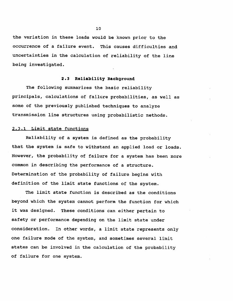
The limit state function is described as the conditions
beyond which the system cannot perform the function for which
it was designed. These conditions can either pertain to
safety or performance depending on the limit state under
consideration. In other words, a limit state represents only
one failure mode of the system, and sometimes several limit
states can be involved in the calculation of the probability
of failure for one system.

11
For the specific case of the transmission line structure,
the structure is designed for the function of supporting the
conductors, which are attached to the structure by an
insulator assembly. For clarification, the insulator
assembly is shown in Fig. 2.1.
Some examples are listed below of the transmission
structure failure modes where it fails to serve its purpose in
supporting the conductors:
• elastic instability of the structure • forces in a component beyond its capacity • formation of a mechanism resulting in a large rotation
that results in a collapse of the transmission structure.
290 LBS PD I.SST
BUllDLI CONDUCTORS
• • .... .. ..
- 5(8"
• • :.==~~ ~ = :::~ i ~ .... ....
• 5
7
ITEM
1
2
3
4
5
6
7
QTY DESCRIPTION
1 . ANCHOR SHACKLI
1 OVAL BYE BALL
18 INSULATOR UNITS
1 SOCKET "Y" CLEVIS
2 IYE "Y11 CLEVIS
2 SUSPENSION CLAMP
1 YOKI PLATE
Fig. 2.1: A typical insulator assembly.

12
Each type of failure listed above constitutes a different
limit state.
The limit state function, G, is based on the difference
between the random structural resistance variable, R, and the
load variable, Q, which is numerically shown as:
G = R{x)-Q (2. 1)
where xi represent the geometric and material parameters that
are used to evaluate the resistance, R. More details
concerning the procedure used in this work will be discussed
in the next chapter.
2.3.2 Levels of analysis
Once the limit states are stated in terms of the
variables, xi, the calculation of the probability of failure
is accomplished on one of three levels. Each level has a
progressively higher level of sophistication with respect to
the analysis procedure. In the following, discussion will
progress from the highest level (level 3) to the lowest level
(level 1). The highest level is the most complete and
accurate representation of the computation of the probability
of failure.
2.3.2.1 Level 3: reliability analysis
At level 3, the probability of failure is measured by a
multidimensional integration of the joint probabilities of the
resistance and load. Letting fR(r) characterize the density

13
fR(r). fq(q)
Load, Q Resistance, R
p1
= P(R<Q) ~ r,q
Fig. 2.2: Fundamental reliability problem.
function of the resistance, and fQ(q) denote that density
function of the load, the integration of the following
equation results in the exact probability of failure:
• q
Pt=P(Rs.Q) = J fo(q) J fR(r) drdq (2. 2)
The graphical representation of the probability distributions
of the resistance and the load is shown in Fig. 2.2, with the

14
area portraying the probability of failure, Pf r also being
indicated.
This computation requires full knowledge of the
distribution functions and is extremely difficult to evaluate;
the complexity of this computation even renders many cases
impossible to evaluate. For this reason, Monte Carlo
simulation methods are more common. These methods simulate
finite values of the resistance and load to find the
probability of failure utilizing computer analysis. However,
this approach requires a large number of runs (3000 to 4000,
according to Ref. 16) to produce a statistically reliable
probability of failure, which may be very time consuming.
2.3.2.2 Level 2: reliability analysis
Due to the deficiencies of level 3, level 2 methods make
assumptions and simplifications in order to make the
calculation of the probability of failure easier. The
sacrifice of making these simplifications results in an
approximate value for the probability of failure. The essence
of level 2 methods entail checking a finite number of points
(usually only one point at the mean values of the variables)
on the limit state function surface. For comparison, level 3
involves checking of all points along the entire surface of
the limit state function.

15
2.3.2.3 Level 1: reliability analysis
Level 1 entails the most simplistic approach of all
three. This approach encompasses design and safety checking
methods, because only a single characteristic value is
connected to each variable. In actuality, no probability of
failure calculations are performed; so level 1 methods are not
really methods of reliability analysis (8]. However, level 1
operational methods provide engineers with a basis for design
code provisions.
Level 2 balances the disadvantages and benefits involved
in the calculation of the probability of failure better than
the other levels; accordingly, it is the focus of. this
research. Within level 2, the particular method that will be
applied to this work is the First Order-Second Moment (FOSM)
method.
2.3.3 Reliability analyses of transmission line structures
Due to the different reliability levels of analysis and
various methods available within each level, numerous
reliability methods have been applied to the analyses of
transmission line structures. Details of some of these
methods will be discussed in this section.
2.3.3.1 Reliability relationship between line and structure
The system reliability may refer to the entire
transmission line encompassing miles of transmission

16
structures, or to a single transmission line structure. In
the first case, the reliability analysis must not only
consider the variation of the load processes that affect the
line, but also the spatial correlations within and among these
load processes.
A method for relating the reliability of these two
aspects of system, (the transmission line and the transmission
structure), has been developed by Dagher, Kulendran, Peyrot,
and Maamouri [15). This method calculates the probability of
failure of a line segment, PFL, as
PFL = a (N/n) PFs
where, PFs= probability of failure of a structure, a = system reliability usage factor, N= total number of structures in line segment, and
(2. 3)
n= number of structures simultaneously subjected to the same extreme climatic event.
This relationship accounts for the spatial extent of the
extreme loading events within the system reliability usage
factor, a. The factor, a, is obtained in this source by using
Monte Carlo simulation for extreme wind and extreme ice
loadings.
This analysis was able to use available weather data to
estimate the probability of failure of the line by converting
the problem from an event-based formulation to an extreme
value analysis.

17
2.3.3.2 Monte Carlo example
Level 2 techniques are most frequently implemented, but
level 3 is often employed when Monte Carlo simulations are
needed to validate level 2 methods.
A censoring technique for Monte Carlo simulations was
proposed by Kamarudin [16] that reduced the number of
simulations, and thus reduced the cost and time involved in
analysis. The benefit of the censoring technique is the
ability to determine if individual trials are failures or
survivals without going through the structural calculations.
The amount of savings involved with this procedure is
variable, but may be as much as a 30% reduction of the amount
of computations. Kamarudin tested this technique on a wood
pole design.
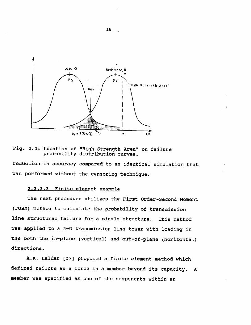
This technique involved checking the resistance of the
structure during each trial and deciding if further structural
calculations were required. If the resistance satisfied a
predetermined check-point criteria, then it was counted as a
non-failure. This check-point is located on the failure
probability distribution (see Fig. 2.3) at line a-a. The area
to the right of the line a-a was considered as the "High
Strength Area". When the resistance was located in this area,
it satisfied the pre-determined check-point, and the
simulation counted as a non-failure.
This procedure was applied to a wood pole design with no
18
Load, Q Resistance, R .. ,...-.---.._
~. "High Strength Area"
Pr= P(R<Q) ~ r,q
Fig. 2.3: Location of "High strength Area" on failure probability distribution curves.
reduction in accuracy compared to an identical simulation that
was performed without the censoring technique.
2.3.3.3 Finite element example
The next procedure utilizes the First Order-Second Moment
(FOSM) method to calculate the probability of transmission
line structural failure for a single structure. This method
was applied to a 2-D transmission line tower with loading in
the both the in-plane (vertical) and out-of-plane (horizontal)
directions.
A.K. Haldar (17] proposed a finite element method which
defined failure as a force in a member beyond its capacity. A
member was specified as one of the components within an

19
individual transmission structure.
The equations used for the horizontal and vertical
loadings due to combined wind and ice at the conductor
attachment points are listed below:
where, PH= Pv= de= t= GF= Co= v= WN= we= WT=
horizontal load, vertical load, diameter of conductor, ice thickness, span reduction factor, drag coefficient, wind velocity, wind span, bare weight of conductor, and weight span.
(2. 4)
(2. 5)
The finite element method utilized a first-order Taylor's
series expansion to find the mean internal stress, s, and the
standard deviation of the internal stress, as, of each member
in the transmission structure. The mean internal strength,
R, was then derived from standard mechanics of materials
equations, and the standard deviation of the internal
strength, aR, was assumed.
A normal distribution was also assumed for these
variables, (S, R, as, aR), which were then used to calculate
the probability of failure, Pf ,i' of each member of the
transmission structure by the following equation:
where B is defined as the reliability index and ~(-B) can be

20
=cj>[-(R-8)] =cj>(-~) ../a~+a2s
obtained from the standard normal table (17].
(2. 6)
Then the Pf,i's were combined to· form lower and upper
bounds, assuming total independence and total dependence,
respectively, on the probability of failure of the structure
in the next equation:
(2. 7)
where Pf is the probability of failure of the structure, and M
is the number of failure modes, or in this case, the number of
members of the transmission structure.
This procedure was applied to an example transmission
structure and sensitivity studies of the various input
statistical parameters (e.g., loading, strength and sectional
properties) were performed. One of the results of the
analyses indicated that the failure probability of the
structure increased by taking into account the effects of
correlation between wind speed and ice thickness.
2.3.3.4 Plastic collapse failure example
A method proposed by Murotsu, Okada, Matsuzaki, and
Nakamura (18] was specifically generated for the failures
produced by large nodal displacements due to plastic collapse
of the structure. This method was applied to a 2-D

21
transmission line structure similar to the structure in the
previous example.
The load equations for this method were given for wind,
snow and tension loads, in which the wind load, Lw' and snow
load, Ls, are listed below:
where, p= G= v= Co= D= t= S= H= Pe=
L,, = ~p(Gv) 2 CD (D+2t) S (H/lO) Y'
air density, gust factor, winter average wind speed at site of structure, drag coefficient, conductor diameter, snow thickness, span length, height at which wind acts, and snow density.
(2. 8)
(2. 9)
The tension loads, LT, were determined by solving a non-linear
equation which accounted for a maximum allowable stress of
conductors , wind speed, snow thickness and temperature.
Then the horizontal and vertical loads acting on the
conductor at its attachment point to the arms of the structure
were calculated from Lw, Ls, LT, and the angle of the
conductors with respect to the surrounding structures.
A structural analysis using the direct displacement
method was performed. For the given failure criteria and a
transmission line structure with many degrees of redundancy,
structural fa i lure results only after the yielding of sever al

22
components within the transmission structure. To de.termine
the system failure probability, one must investigate all
possible failure mechanisms. However, this seems impractical
to include all of these mechanisms, particularly in a highly
redundant structure. Therefore, a procedure was used which
selected the probabilistically significant failure paths.
This selection process was accomplished with the branch-and
bound technique. For details related to this method, the
reader is referred to Ref. 18.
This method was then successfully applied to a
transmission line structure, and the dominant failure mode was
found to be the side~sway mechanism of the top portion of the
structure.
2.3.3.5 Newfoundland transmission line failure
Two major line failures occurred in 1980 and 1987 to the
transmission line which runs along the west coast of
Newfoundland. As a result, The Transmission Design Department
of Hydro undertook a detailed study on the assessment of the
existing line reliability and the course of action that is
necessary to increase the level of reliability of the line
(19].
The transmission tower of interest is a suspension-type,
guyed-v tower, which means the structure is in the shape of
the letter "V". The study included the analysis of the
existing and upgraded structure under various basic climatic

23
loading conditions. The upgraded structure was improved by
modifying some members to carry unbalanced vertical ice loads.
The loading condition of unbalanced vertical ice loads was
found to cause failure and contribute significantly to the
probability of failure.
In this study, a total of nine load cases were
considered. Seven of these load cases were related to ice-
only loading while the remaining two load cases were extreme
wind and combined wind and ice loads.
The strength of a member in the structure was taken to be
a random variable and related to the nominal strength, Rn, as
R=MFPRn (2.10)
resistance, variability due to material,
where, R= M= F= P=
variability due to erection and fabrication, professional factor that represents the uncertainties in the strength theory, and
Rn= nominal strength.
The variables M, R, and P were assumed to be uncorrelated
random variables, so the coefficient of variation of the
strength, VR, could be approximated as:
(2.11)
where, VM= coefficient of variation of M, VF= coefficient of variation of F, and

24
Vp= coefficient of variation of P.
In the reliability analysis of this work, some details of
the procedure were not explained. The document states that
interference between the strength, R, and stress, Q, (effects
of various loads) was taken into account using the
mathematical theory of probability (19). From that point, the
reliability of the tower &rower was computed based on the
assumption that an individual member fails either in tension
or in compression mode. Therefore, these two events are
mutually exclusive under a particular load case. Members were
grouped according to the particular mode of failure and total
reliability of the structure was given as:
n m
RTower = en Rei> ( II RTj> i .. 1 j•n+l
reliability of an individual member, i, in compression,
(2 .12)
reliability of an individual member, j, in tension, total number of members under consideration.
Assuming the load case events are independent, the
estimate of the structure lifetime failure probability was
given by:
M
~ P(N.) Pt · Li .1 ,J.. (2.13)
i=l

where, pf, i =
25
probability of failure given that the "load case i" occurs, probability of occurrence of this load case, and number of load cases.
The results of this analysis indicated that the existing
structure has an annual probability of failure of 0.0096, or
approximately 1 out of 100. The annual probability of failure
for the upgraded structure was calculated to be 0.0073, or 7
out of 1000.
An economic analysis was also conducted in which the
initial cost of the line is balanced against the future
failure costs. The final results indicated that shortening of
the existing span by adding structures is the most economical
solution for upgrading this line.
The focus of this work is on the development of the limit
state function, G{x}. The methods discussed in this chapter
involve complicated equations and procedures to produce this
equation. Development of the limit state function was
accomplished in the next chapter, Chapter 3, by using a
regression technique.

26
3. DESCRIPTION OF THE PROCEDURE
As shown in the previous chapter, numerous approaches to
a reliability analysis have been documented. In this chapter,
the method utilized to construct a fragility curve for a
transmission line structure is developed. The calculation for
the structure's probability of failure includes all possible
failure modes that may affect the structure's performance.
This analysis involves the following three steps:
1. Determination of the failure functions for possible failure modes.
2. Calculation of the probability of failure for each mode.
3. Combination of the individual modes failure probabilities to obtain the structure's probability of failure.
3.1 Development of the Failure Functions
A failure function defines the point at which a
structural element fails to perform its function and is
expressed as:
( 3. 1)
where xi represents the geometric and material variables that
affect an element resistance, R, and Q is an applied load.
The resulting magnitude of G{x} determines the presence of a
safe or failure region. For example, G{x} > o indicates a
safe region, and G{x} < O denotes a failure region.
Formulation of G{x} consists of using a closed form

27
solution. However, in most cases, this is a formidable task,
particularly when dealing with complex systems such as
transmission lines. Although some researchers have utilized
finite element techniques (see Haldar (17) and Murotsu, et al.
(18]), these techniques involve a significant number of
rigorous analyses to incorporate the indeterminacy of the
structure.
3.1.1 Generation of data points
Alternately, in the method proposed herein, G{x} can be
derived by using a technique similar to a Monte Carlo
simulation. This technique is advantageous because it does
not require finite element analysis. In the following
sections, the goal is to represent the failure regions with
the minimum number of structural analyses and to use these
representations to estimate the system failure probability.
This method was developed using the principles described in
Ref. 5.
In this procedure, a set of data points on the failure
surface is estimated. The size of the set of data points is
arbitrary but must have more data points then the number of
variables in order for the regression analysis to be
performed. Also a larger data set will result in a better
estimate of the failure function. A regression technique is
then employed to formulate the failure function. Estimation
of the data points on the failure surface was accomplished

28
using two similar methods . The procedure of these two methods
will be outlined in the example problems in Section 3.4.
3.1.2 Regression analysis
Regardless of the method of generating the data points,
regression analysis is required to develop the limit state
equation. Each group of data points associated with an
individual failure mode were analyzed (or regressed) to
determine the failure equation, G{x}, for each failure mode.
The regression analysis was accomplished by using the
statistical analysis program SAS [9]. This program uses the
method of least squares to fit the generated equations. An
example input file for the SAS program is presented in the
following example in Section 3.4.1.
Each equation that was obtained was checked for
independence between the residuals and the predicted values,
and normality of the residuals. These checks confirm that the
generated failure equation is an accurate representation of
the data.
3.2 Reliability Analysis: First order-second Moment Method
As stated in the Chapter 2, the First Order-Second Moment
(FOSM) method was used to calculate the probability of
failure, Pf, for each possible failure mode, i.e.,:
Pt=P(G(x}~O) (3.2)

29
3.2.1 Reliability index
The calculation of the probability of failure involves
determination of a reliability index (often called the safety
index), B, defined as:
(3. 3)
where µG represents the failure function, G{x}, evaluated at
the mean values of the variables, and aG is the standard
deviation of G{x}. Equation 3.3 may also be expressed as
(3.4)
This is illustrated in Fig. 3.1 where the probability density
function is shown for G. The shaded area to the left of the
vertical axis is equal to the probability of failure. If the
mean, µG, is moved to the right and aG is held constant, the
probability of failure is reduced. Hence, increasing the
value of B corresponds to a reduction in failure probability
or an increase in reliability.
The relationship between B and the probability of
failure, Pf, can be established by approximating the
distribution of G{x} as a normal distribution (7], hence Pf
can be calculated as:
(3.S)
where t is the standard normal integral which can be estimated

30
pf 0 µg g
I. B crG .I Fig. 3.1: Graphical illustration of reliability index.
the available normal distribution probability table. There
are several techniques to calculate 8. In this research, the
Lind-Hasofer method [7,8] was used. Details concerning this
method are given in the next section.
J.2.2 Calculation of reliability index: Lind-Hasofer Method
When the failure function, G{x}, is non-linear, problems
are encountered in calculating the safety index, B. In this
case, the FOSM methods account for the non-linearity by
linearizing only a point on the failure boundary surface,
referred to as the design point, {x*}. The procedure is
iterative and involves recalculating the design point several
times and linearizing G{x} at each point.

31
The Lind-Hasofer method is used in this study since it is
the basis for most methods [6]. This method can be described
in two steps: (1) transformation of the random variables,
{X}, into a space of reduced variables, {Y}, by
(3.6)
and (2) measuring, in the transformed space, the shortest
distance between the origin of the space to the failure
surface. This concept is illustrated in Fig. 3.2 for a two
parameter failure function.
The reliability index, B, is defined as the minimum
distance between the origin and the failure surface in the
transformed space. The design point now becomes {y*} and
represents the "most likely" point of failure. Calculating
the design point requires solving a minimization problem. A
numerical solution is defined by the following system of
equations, with respect to the original variable space of
independent random variables, {X},
{a) = A. [a xl {VG)
{x•) = {µ xl- p [a xl {a}
G{x•) = 0
(3.7)
(3.8)
(3.9)
( 3 .10)
in which {VG} are the gradients of G evaluated at the design

G < 0 FAILURE
a.) ORIGINAL COORDINATES
32
G > 0 SAFE
._ ___ G = 0
SAFE DOMAIN //
FAILURE DOMAIN
b.) REDUCED COORDINATES
,.."8
Fig. 3.2: Original and reduced variable coordinates in reliability analysis.

33
point {x*}, and {a} is the vector containing the direction
cosines of the random variables.
The Lind-Hasofer method is slightly modified to account
for random variables with non-normal distributions. This can
be accomplished by transforming the non-normal variables into
reduced normal variables prior to the solution of the
minimization problem [7]. The transformation process involves
the determination of the mean and standard deviation of an
equivalent normal variable, µxiN and axiN• These are found
under the conditions that the cumulative distribution and
probability density function of the non-normal and
approximating normal variable are equal at the design point,
{x*}. This leads to:
4> (4>-1 [Fx, (xj)] ) = ~~~~.;;__~~-
where Fxi(.) and fxi(.) denote the actual cumulative
distribution and density distribution of the non-normal
variable, Xi .
An iterative procedure to calculate the reliability
index, B, is summarized in Ref. 7 as follows:
1. Define the limit state function [Eq. (3.1)].
(3.11)
(3.12)
2. Approximate an initial value of the reliability index, B.
I
I

3.
4.
5.
6.
7.
8.
9.
34
Set the initial design point values {x*} = {µx}·
Compute µxiN and a~iN for those variables that are non-normal according to Eqs. (3.10) and (3.11).
Calculate partial derivatives, {VG}, evaluated at the design point, {x*}.
Compute the direction cosines, {a}, from Eq. {3.6).
Compute new values of {x*} from Eq. (3.7) and repeat steps 4 through 7 until estimates of {a} stabilize.
* Compute the value of B necessary for G{x } = O.
Repeat steps 4 through 8 until the values of B on successive iterations are within an allowable tolerance.
When a satisfactory value of the minimum distance, B, is
obtained, the failure probability, Pf, can be evaluated from
t(-B).
3.3 Multiple Failure Functions
The previous sections describe the generation of the
failure functions, G{x}, and the calculation of the
probability of failure from G{x}. In this section, the
computation of the structural probability of failure is
discussed.
Once the failure modes and associated probabilities are
established, the system probability of failure is calculated.
This computation involves the statistical union (U) of the
individual modes of failure, i.e., the system failure
probability can be expressed as:
where n is the number of failure modes.

35
(3.13)
The exact calculation of Pf requires the determination of
the correlations between all of the failure modes. If more
than two failure modes are considered, calculating the
correlations, and incorporating it into the probability of
failure equations is a tedious task. Therefore,
simplifications are employed to calculate upper and lower
bounds instead of the exact probability. For example,
assuming that independence among the failure modes, the upper
bound failure probability is:
n
Pf= 1-IJh-P[F;J} (3.14) i•l
for small P[Fi], the formula may be simplified to
n
Pf= L P[F;l (3.15) i•l
The lower bound failure probability is calculated based
on the assumption that the failure modes are dependent on each
other which corresponds to th.e largest failure probability
among the individual modes. The lower bound failure
probability is shown below as:
Pf= max P[F;l (3.16)
For a large and complex structure, derivation of all of
the failure modes including the modes that have a very small

36
probability of occurring, may be very time consuming.
Therefore, one may consider only the dominant failure modes.
This will not significantly jeopardize the calculation of the
system calculation of the probability of failure. This will
be illustrated in the ten-bar truss example in the next
section, Section 3.4.2.
3.4 Examples Problems
3.4.1 Ten-bar truss
In this technique, an iterative process to obtain a set
of data points is used. The procedure consists of increasing
the applied loads until a component in the structure reaches
its structural ultimate strength. The structure is then
modified by constraining the forces of the failed component to
its estimated ultimate strength and reanalyzing the system to
predict the next component to fail. These steps are repeated
until a system failure is attained.
This process also involves random generation of the
system variables that define the strength of all structural
members. Assuming a normal distribution, a random generator
that utilizes the mean and standard deviation can be used to
generate random values for the system variables. This step
was accomplished using the normal random number generator in
the Minitab software statistical program (21]. Minitab is
also capable of generating random numbers with other
r
I

37
distributions such as the Weibell and Poisson distributions.
The proposed method is a simulation technique but differs
from Monte Carlo simulation. The simulation runs in this
method are used to formulate the limit state, whereas in a
Monte Carlo simulation the probability of failure is directly
calculated. Also, the number of analyses in Monte Carlo
simulation (in the range of 10,000) greatly exceeds the number
of analyses used for this method (in this case 29).
To demonstrate this procedure the ten-bar truss system,
shown in Fig. 3.3 [8,22], was used. The basic variables in
this example are the individual element resistances which are
considered statistically independent and characterized by a
normal distribution. The mean values of each element
resistance, Ri, are listed in Table 3.1. A coefficient of
variation for each element resistance is assumed as 0.2.
Component failure results when the axial load in the
member reaches the member ultimate capacity leading to
failure. System failure occurs when the structure reaches an
unstable stage. One should notice that failure of elements 1,
3, 7, or 10 result in an unstable structure and hence a system
failure. Therefore, the analysis is a lot simpler and must be
concluded when any of these members fail.
Reliability analyses of the ten-bar truss was
accomplished by analyzing the structure 29 times. Each of the
29 analyses resulted in one of five failure modes. Overall,

38
4
1 7
~f<-~-1;..._~-5
-f-~~2::_~---'lf--~~~~ _ __. .. , ... ,___ 3 _ __. .. ,, _____ 3 --1
4P
16P
Fig. 3.3: Ten-bar truss example problem.
Table 3.1: Mean resistances for the truss elements in Fig. 3.3.
ELEMENT ELEMENT NUMBER MEAN RESISTANCE (kips)
1 15
2 15
3 15
4 15
5 20
6 20
7 25
8 10
9 10
10 25
39
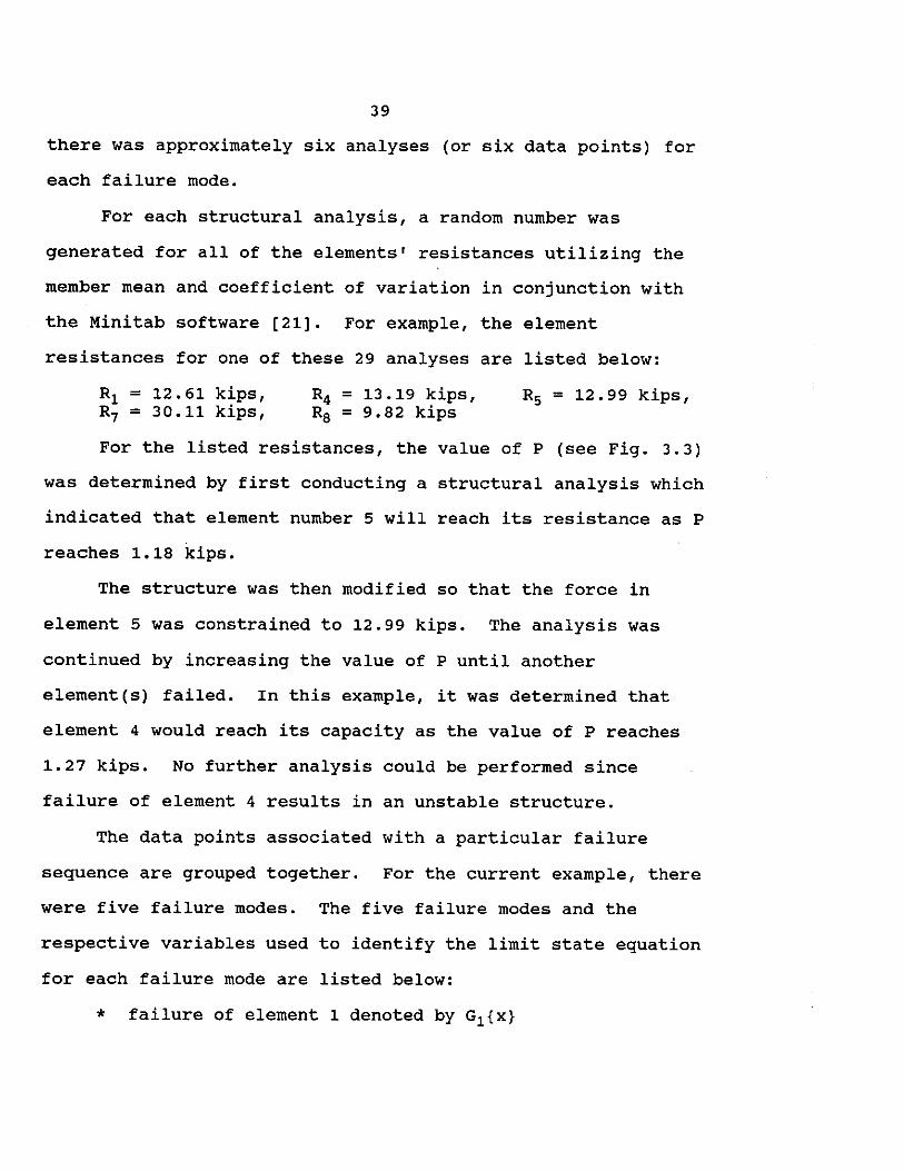
there was approximately six analyses (or six data points) for
each failure mode.
For each structural analysis, a random number was
generated for all of the elements' resistances utilizing the
member mean and coefficient of variation in conjunction with
the Minitab software (21]. For example, the element
resistances for one of these 29 analyses are listed below:
R1 = 12.61 kips, R7 = 30.11 kips,
R4 = 13.19 kips, R8 = 9.82 kips
R5 = 12.99 kips,
For the listed resistances, the value of P (see Fig. 3.3)
was determined by first conducting a structural analysis which
indicated that element number 5 will reach its resistance as P
reaches 1.18 kips.
The structure was then modified so that the force in
element 5 was constrained to 12.99 kips. The analysis was
continued by increasing the value of P until another
element(s) failed. In this example, it was determined that
element 4 would reach its capacity as the value of P reaches
1.27 kips. No further analysis could be performed since
failure of element 4 results in an unstable structure.
The data points associated with a particular failure
sequence are grouped together. For the current example, there
were five failure modes. The five failure modes and the
respective variables used to identify the limit state equation
for each failure mode are listed below:
* failure of element 1 denoted by G1{x}

40
* failure of element 7 denoted by G7{x} * failure of elements 4 and 5 denoted by G4, 5 {X}
* failure of elements 5 and 8 denoted by Gs,a{x} * failure of elements 4 and 8 denoted by G4, 9{X}
The list of generated data points is located in Table 3.2 in
which the data points are grouped by failure modes. Regression
analysis of each group of data points was performed using the
SAS software (9]. An example SAS program for the calculation
of the limit state equation, G4, 5{x}, is located in Fig. 3.4.
This program include the data points which are highlighted in
Table 3.2. The output from this program is shown in Fig. 3.5
and can be interpret by taking note of the figures indicated
in Fig. 3.5. These figures are the estimates of the
coefficients for the corresponding variables as denoted in the
"Parameter" column, which is also indicated in Fig. 3.5. The
SAS program computes the equation:
P= 0. 0555694124 X4 + 0. 04167 08885X5 (3.17)
The limit state equation has all the variables on one side of
the equation, so rearranging and rounding of the variables
results in the limit state equation for failure of elements 4
and 5 as:
G4 , 5lx) = 0.0556R4 + 0.0417R5 - P (3.18)
The equations for the remaining failure modes are calculated
in the same manner and are listed below:

41
Table 3.2: Data points for ten-bar truss example.
P (kips) R1 (kips) R5 (kips)
FAILURE OF ELEMENT 1
1.16 10.40 12.75 22.85 25.29 8.05
0.96 8.64 16.70 21.·05 30.09 7.93
0.98 8.80 12.61 12.99 30.11 9.82
1.09 9.82 16.42 20.56 28.09 8.61
1.11 9.99 14.52 16.79 28.42 11.43
1.44 12.99 17.65 20.29 40.22 11.03
FAILURE OF ELEMENT 7
1.38 18.00 16.09 18.41 20.67 10.11
1.28 20.24 17.79 17.77 19.19 8. 38
1.12 14.83 22.18 21.54 16.84 8.51
1.41 18.15 13.30 25.40 21.21 10.00
1. 38 18.85 19.06 22.78 20.62 12. 65
1.50 27.13 20.95 20.72 22.56 13.07
FAILURE OF ELEMENTS 4 AND 5
.... . y ];~··4jL ..••.••. 1<.····i~•Jl$z.l··••<•:Id~o'it•· i i s}fcj·\··•· I.• >/~~·····<.c; •.. •···· 11.43 ... .
···· · 1.sa. t >Ir•• >:i3L61Fr··, \ iiif.1.6 r < ··•·••· >~ :J;!io?··• ·• ··.•···~·o.;i2 ./ ····./.1.1.}03 ..... ····. ·····•····<J..·50 <+s.(i?r . •·•·• >14<ab . /i~<l.2.······•·••·· .· .. ·····• $1.;$c;/ ..•..•. ·· {t.~.~
FAILURE OF ELEMENTS 5 AND 8
1.49 15.00 15.00 15.90 25.00 10.0
1.66 16.45 20.07 18.41 25.89 10.11
1.53 20.71 15.40 17.77 30.29 8.38
1. 66 14.94 17.59 25.40 31. 87 10.00
1. 71 19.36 17.39 18.78 25.97 10.65

42
Table 3.2 (cont.)
p (kip) R, (kip) R4 (kip) Ro; (kip)
1. 61
1.38
1. 32
1. 48
1. 76
FAILURE OF ELEMENTS 4 AND
15.00
12. 75
16.70
13.78
17.01
11 JOB //SAS EXEC SAS //DD SYSIN **
DATA FAIL45;
15.00
13 .12
12. 69
14.22
15.20
INPUT P X4 X5;
CARDS;
1.27 13.19 12.99 1. 44 10.49 20.56 1.43 13.07 16.79 1.58 13.16 20.29 1.59 14.80 18.12 1.71 13.22 23.59 1.67 13.85 21.54 ;
PROC GLM; MODEL P=X4 X5;
20.00
22.85
21. 05
18.46
22.28
R7 (kip) RA (kip)
8
25.00 8.90
25.29 7.05
30.09 7.93
23.85 8.92
27.06 7.78
OUTPUT OUT=NEW PREDICTED=YHAT RESIDUAL=RESID;
PROC PLOT; PLOT RESID*YHAT;
PROC SORT; BY RESID; DATA NPLOT; SET NEW; N+2; NS=PROBIT((N-1)/14);
PROC PLOT; PLOT NS*RESID;
Fig. 3.4: SAS program used to perform regression analysis.

43
General Linear Models Procedure
Dependent Variable: p
Source DF Sum of Squares Mean Square F Value Pr > F
Model 2 0.14257569 0.07128784 99999,99 0.0001
Error 4 0.00000000 0.00000000
Correct~d Total 6 0.14257569
R-Square c.v. Root MSE
1.000000 o. 001011 0.00001543
Source DF Type I SS Mean Square F Value Pr > F
X4 0.01740105 0,01740105 99999.99 0.0001 XS 0.12517464 0.12517484 99999.99 0.0001
Source OF Type III SS Mean Square F Value Pr > F
X4 0.03116393 0.03116393 99999.99 0.0001 XS 0.12517464 0.12517484 99999.99 0.0001
T for HO: Pr > T Parameter Estimate Parameter=O Estimate
INTERCEPT -.0002481606 -3.24 0.0317 0.00007660
I~! 0.65556§41241 11443. 77 0.0001 o. 00000486 0.041670888~ 22935. 13 0.0001 0.00000182
Fig. 3.5: Output from SAS program in Fig. 3.4 used to develop the limit state equation, G4, 5 {x}.
(3.19)
G7 {x) = 0. 067 R, - P (3.20)
G5 , 8{x) = 0. 0624 R5 + 0. 05R8 - P (3.21)
G4 , 8{x) = 0 .1624R4 + 0 .101R8 - P (3.22)
Knowing the failure function for each mode, one can
calculate the probability of failure, Pf, utilizing the FOSM
method (see Section 3.2). A spreadsheet was used to for these
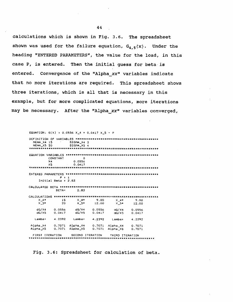
44
calculations which is shown in Fig. 3.6. The spreadsheet
shown was used for the failure equation, G4, 5{x}. Under the
heading "ENTERED PARAMETER.S", the value for the load, in this
case P, is entered. Then the initial guess for beta is
entered. Convergence of the "Alpha_xx" variables indicate
that no more iterations are required. This spreadsheet shows
three iterations, which is all that is necessary in this
example, but for more complicated equations, more iterations
may be necessary. After the "Alpha_xx" variables converged,
EQUATION: G(X} = 0.0556 X_4 + 0.0417 x_s - p
DEFINITION OF VARIABLES ******************************************* MEAN_X4 15 SIGMA_X4 3 MEAN_XS 20 SIGMA_XS 4
*******************************************************************
EQUATION VARIABLES CONSTANT X4
************************************************ 0
0.0556 XS 0.0417
*******************************************************************
ENTERED PARAMETERS ************************************************ p ; l
Initial Beta = 2.83
CALCULATED BETA *************************************************** BETA= 2.83
CALCULATIONS *****************************~************************ X_4* IS x -·· 9.00 x _4• 9.00 X_5* 20 x _s• 12.00 x - s• 12.00
dG/X4 0.0556 dG/X4 0.0556 dG/X4 0.0556 dG/XS 0.0417 dG/XS 0.0417 dG/XS 0.0417
Lamba= 4.2392 Lamba= 4.2392 Lamba= 4.2392
Alpha_X4 0.7071 Alpha_X4 0.7071 Alpha_X4 0.7071 Alpha_ XS 0.7071 Alpha_x5 0.7071 Alpha_xs 0.7071
FIRST ITERATION SECOND ITERATION THIRD ITERATION *****************************************************************
Fig. 3.6: Spreadsheet for calculation of beta.

45
then the task is to change the "Initial Beta" until it
converges with the calculated "BETA". For a linear equation
such as G4, 5{x}, the "Initial Beta" does not alter the
calculation of "BETA", but for more complex equations, this
step is necessary.
The bounds of the failure probability can then be
estimated using Eqs. (3.15) and (3.16) (see Sections 3.3).
The results of this analysis are compared to the results
obtained by Knapp (8) who used 19 failure modes (see Fig.
3. 7) •
The proposed method to calculate a system failure
probability while considering fewer failure modes proves to be
close to the estimations obtained in (8). This demonstrates
that one needs to use only the dominate failure modes to
obtain the fragility curve for the structure.
In the technique demonstrated above, the user needs not
know the failure sequence prior to analyzing a structure.
Therefore, in order to group together enough data points for a
specific failure mode, the values of some of the randomly
generated variables can be "directed", (i.e. weakened or
strengthened). More specifically, the weakening or
strengthening of a variable means that the mean value is
increased or reduced in the random number generator as a way
of forcing certain failure paths.
The use of the "directing" technique does not guarantee

-c.. ~-:::J
10·1
·;;; 10-2 --0 >
.'!:::
..0
'° ..0 e c..
I g 0
0.5
46
0
O FOSM WIDE BOUNDS ) O FOSM NARROW BOUNDS KNAPP'S(8] -~- MONTE CARLO RESULTS
951 Clllfileu:e .....
- - - METHOD 1 BOUNDS
1.0 Load,q
1.50
Fig. 3.7: Fragility curve for ten-bar truss example.

47
that all failure modes with high-probability will be
identified and included in the analysis. This is a
disadvantage of this procedure. Also the user is expected to
interpret the information from the structural and statistical
analyses and to recognize which elements to "direct" either by
weakening or strengthening. As a result of this disadvantage,
the technique listed below was examined, which is a more
systematic way to identify the failure modes.
3.4.2 Portal frame
This approach for generating data points on the failure
surface is more specific than Method 1. Instead of generating
resistance variables, the applied loads were randomly
generated. Then, the structural analyses were performed, and
the resulting member forces were recorded.
The user determines the failure modes needed for
estimating the system reliability. In contrast to the
previous method (Method 1), the failure modes were unknown
prior to the completion of all the analyses. Some
simulations using Method 1 resulted in modes that were not
included in the probability of failure calculation. Method 2
eliminates those structural analyses; therefore, less
simulations were necessary to accumulate enough data points
for the same failure mode.
(The 29 analyses cited in Section 3.4.1 did not include
the extra analyses which did not contribute information to the

48
example. Since the time for each structural analysis for that
example is so insignificant, the irrelevant analyses were
disregarded instantaneously and a count of them was not
possible.)
The above procedure (Method 2) is first demonstrated,
then verified. The demonstration utilized the portal frame
shown in Fig. 3.8 [8]. Verification of Method 2 was also
conducted using the previous ten-bar truss example.
In the portal frame example, elastic-perfect plastic
material properties were assumed. Structural failure is
defined when a collapse mechanism is formed. The random
variables are the loads, P1 and P2 , and the plastic moment
capacity of each element is Ri. The variable, Ri is the
plastic capacity of the section located at the joints in Fig.
3.8. The mean values and coefficient of variation for these
variables assuming a normal distribution are listed in Table
3 • 3 •
The first step was to identify the failure sequence. For
example, Fig. 3.9 shows all the possible failure mechanisms
for the portal frame in Fig. 3.8 . To illustrate this method,
the mechanism involving the beam failure (i.e., the formation
of plastic hinges at location 2, 4, and 7) was considered .
Next, random loads were generated for P1 and P2 using
Minitab [21] (see Table 3.4). Ten values were generated for
ten analyses. The loads were used to analyze the portal frame
49
2m
4m
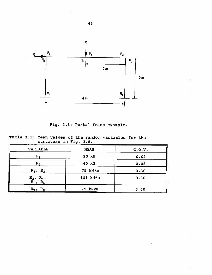
Fig. 3.8: Portal frame example.
Table 3.3: Mean values of the random variables for the structure in Fig. 3.8.
VARIABLE MEAN c.o.v. P, 20 kN 0.05
p? 40 kN 0.05
R,' Ro 75 kN*m 0.30
R3, R4, 101 kN*m 0. 30 R~, R~
R~, RA 75 kN*m 0.30

50
(I) ,
(21
11 11 1 ($) (6) (7J (8)
(9) (10)
Fig. 3.9: Failure mechanisms for portal frame.
Table 3 4• Random numbers generated for P and P . . . , "? •
Analysis P, (kN) p? (kN)
1 20.00 40.00
2 19.86 48.72
3 21. 41 35.12
4 22.83 25.27
5 17.69 48.50
6 28.39 35.49
7 13.41 43.57
8 11.75 47.18
9 21. 22 25.60
10 23.09 19.90

51
for the first iteration. The structure was then modified by
introducing a hinge and a moment at locations 2, 4 or 7 where
the largest of the three moments occurred. In this case, the
evaluation illustrated that the first hinge will occur at
location 7. The structure was then modified by introducing a
hinge and a moment at location 7 (see Fig. 3.10). This is the
ultimate capacity of the member at this location and was
assumed to be varied for each analysis, so it was defined by
the value calculated from this iteration. For example,
considering Analysis 1 where P1=20 kN and P2=40 kN, the moment
at hinge 7 was 57.44 kN*m, so this was the value of the R7 in
Fig. 3.10.
For the second iteration, the modified structure was
subjected to loads P1, P2 and R7 with the values shown in Table
3.5. The loads P1 and P2 were increased by an arbitrary
amount of 2 kN from the first iteration; while R7 was kept
Fig. 3.10: Modified structure for second iteration.

52
Table 3.5: Applied loads to structure in Fig. 3.10.
Run P, (kN) p? (kN) R7 (kN*m) .... •· ...•...• { i> ,. < 22.,()b ) ·•········· i . \ 42;ho ·• >'-·-' •···•
... ··.·.•.. ·•· < '.·'- -.-. ·=· ,-,_ .. _ :- : ::::/<::,:::<: ... •• .... <s., .• ,... . •>• ··=··=: ·_:··· -·_., _.:. __ •.·.•.·
2 21.86 50.72 65.47
3 23. 41 37.12 54.28
4 24. 83 27.27 46.47
5 19. 69 50.50 63.10
6 30.39 37.49 61.60
7 15.41 45.57 54.15
8 13. 75 49.18 55.92
9 23.22 27.60 45.17
10 25.09 21. 90 41. 69
constant. After the analysis of the modified structure was
completed, the structure was then modified by introducing
another hinge at location 4. The evaluation indicated that
location 4 was the next plastic hinge location. Considering
only Analysis 1 again, the moment was constrained at this
location to 67.83 kN*m (see Fig. 3.11).
For the final step, the structure shown in Fig. 3.11 was
subjected to P1 and P2 with the values shown in Table 3.6.
Loads P1 and P2 were increased again from the previous
iteration, while R4 and R7 remained the same, and the moment
at location 2 was monitored.
Regression of the data points in Table 3.7 was used to
develop the limit state equation as described in Section
3.1.1. Each row in Table 3.7 consists of one data point. The

53
Fig. 3.11: Modified structure for third iteration.
Table 3.6: Applied loads to structure in Fig. 3.11.
Run P, (kN) P? (kN) R7 (kN*m) R4 (kN*m) .•
I 1 32.00 52. 00 ·• .• ·. 57. 44 ... 67.83
2 31.86 60.72 65.47 81.46
3 33.41 47.12 54.28 60.21
4 34.83 37.27 46.47 44.82
5 29.69 60.50 63.10 81.12
6 40.39 47.49 61.60 60.79
7 25.41 55.57 54.15 73.44
8 23.75 59.18 55.92 79.04
9 33.22 37.60 45.17 45.32
10 35.09 31. 90 41. 69 36.41
54
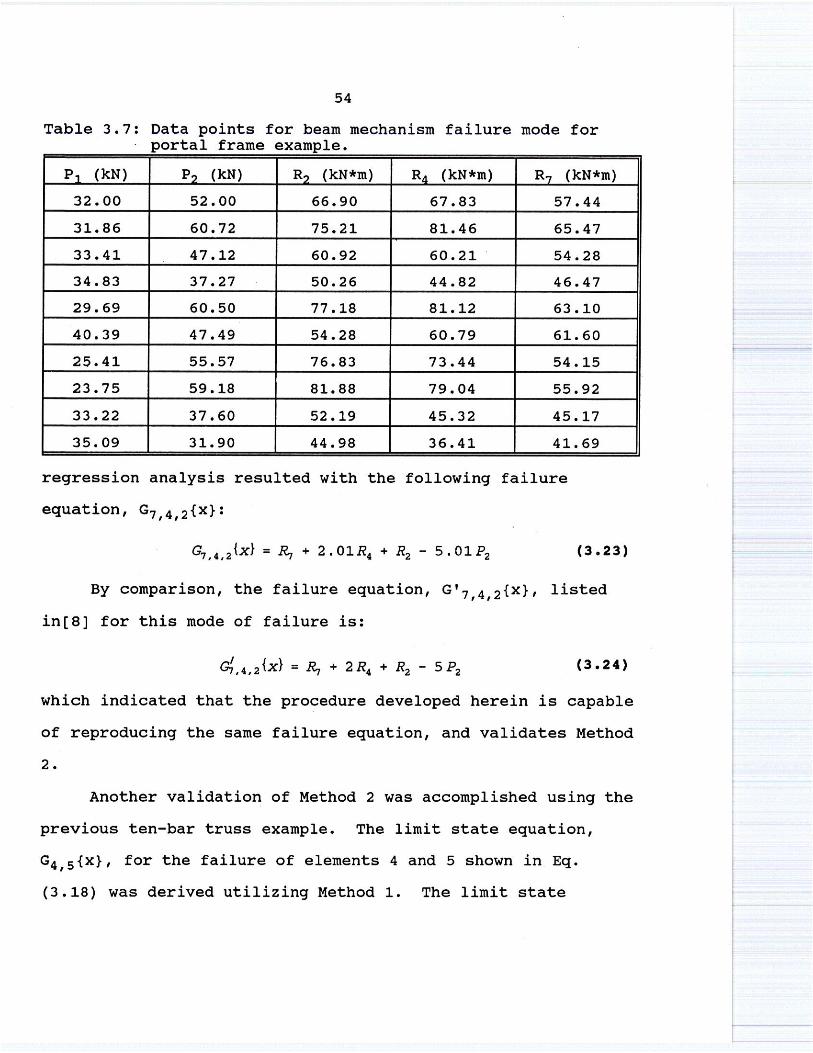
Table 3.7: Data points for beam mechanism failure mode for portal frame example.
P, (kN) p? (kN) R? (kN*m) R4 (kN*m) R7 (kN*m)
32.00 52.00 66.90 67.83 57.44
31.86 60.72 75.21 81.46 65.47
33 . 41 47.12 60.92 60.21 54.28
34.83 37.27 50.26 44.82 46.47
29.69 60.50 77.18 81.12 63.10
40.39 47.49 54.28 60.79 61. 60
25.41 55.57 76.83 73.44 54 . 15
23.75 59.18 81.88 79.04 55.92
33.22 37.60 52.19 45.32 45.17
35.09 31.90 44.98 36.41 41. 69
regression analysis resulted with the following failure
equation, G7 , 4, 2 {x}:
(3.23)
By comparison, the failure equation, G' 7 , 4, 2{x}, listed
in[S] for this mode of failure is:
(3.24)
which indicated that the procedure developed herein is capable
of reproducing the same failure equation, and validates Method
2.
Another validation of Method 2 was accomplished using the
previous ten-bar truss example. The limit state equation,
G4 , 5 {x}, for the failure of elements 4 and 5 shown in. Eq.
(3.18) was derived utilizing Method 1. The limit state
r

55
function for the same failure mode was again developed using
Method 2. This failure equation, G4, 5{x}, was calculated as:
G4 , 5\x) = 0.0556R4 + 0.0417R5 - P (3.25)
Comparing Eqs. ( 3 .18) and ( 3. 2 5) reveals that methods 1 and 2
are the same.

56
4. ANALYSIS OF A TYPICAL TRANSMISSION LINE
The procedure outlined in the previous chapter was
applied to develop a fragility curve for one structure of the
recently failed Lehigh-Sycamore transmission line [3]. The
structure chosen was Tower 281. This tower is one of several
structures that were damaged on October 31, 1991 when a severe
ice storm hit the central part of the state of Iowa (for more
detail, see Chapter 1).
To construct the fragility curve for the failed structure
under ice loading, a computer model was used to analyze a
portion of the transmission line utilizing the ETADS [2]
software. The results were then used in the reliability
analysis previously summarized to estimate the failure
probabilities associated with the different failure modes.
Buckling of the pole, plastic collapse of the pole and cross
arms and insulator failure were considered.
4.1 Finite Element Model
In previous work [1,3], detailed models of transmission
lines consisting of several structures were used to analyze
failed transmission lines to estimate the failure loads. In
this study, a similar but simplified model was utilized. The
model used included only one tower on each side of.Tower 281
and is referred to hereafter as Model 1 (see Fig. 4.1). This
is only an approximate model of a transmission line segment,

57
Tower-280 Tower-281 Tower-282
Fig. 4.1: Model 1 computer model.
but is only used to demonstrate a reliability analysis.
However, if more accurate results are desired, a transmission
line model that includes more structures must be used (3].
In idealizing the structures shown in Fig. 4.1, a fine
mesh of elements was used to model Tower 281. A large
displacement elastic analysis was performed. Linear material
behavior was considered to reduce the computational time.
The effects of material nonlinearity was included in a
model that consisted of one structure. This model is referred
to hereafter as Model 2. In this model, the conductor was
excluded and the forces at the conductor-insulator connections
obtained from analyzing Model 1 were used as input to analyze
Model 2.
4.2 Modelling Assumptions of the Transmission Line system
4.2.1 Geometry
Figure 4.2 illustrates a typical transmission line
structure of the failed line. The towers are H-frame

58
SM
OA IA OA
LEGEND Crose
Item Description section
TL Tower pole 0 IA Inboard arm 0 OA Outboard arm 0 SM Static mast 0 XB X-Braclngs 0 BP Bearing plate
TL TL I Insulator Assembly
GROUND
BP BP
Fig. 4.2: A typical transmission line structure.

59
structures built using hollow tubular steel members. The
structure was assumed to have a fixed base support at the
ground level.
The dimensions and cross-sec.tional properties for Tower
281 are illustrated in Fig. 4.3 and Fig. 4.4. However, the
hexagonal section of the cross-arm was idealized in the model
with an equivalent uniform octagonal section with the same
inertia and cross-sectional area.
The insulator assembly is shown in Fig. 4.5. This
assembly consists of several hardware components with varying
cross-sectional dimensions. Because the insulator units are
allowed to rotate relative to another, its flexural stiffness
was neglected in the finite element model. Hence, these
insulators were modelled as catenary cable elements.
Figure 4.6 illustrates the joint where the inboard arm,
outboard arm, static mast and the tower pole are connected.
This complex joint was simplified in the finite element
idealization assuming a rigid connection also shown in Fig.
4.6.
A plan view of one span showing the conductors and shield
wires modelled in Model 1 is illustrated in Fig. 4.7. The
figure shows that there were three groups of conductors
corresponding to three phases and two shield wires in each of
the spans. The bundled conductor for each phase had two
conducting wires attached to the structure insulators through

60
222 ln.~ 222 In.
390 rn.
I
4"" ~ 240 In.
-i 348 In.
-+ ~"·
276 In.
I
Fig. 4.3: Dimensions for Tower 281.
Ha. (a- 19 In., b•12.7 In., t•6/1S In.)
Hex. (c•13 In., b-8.7 !n., l•3/1S h.)
Oct. (D•1J.1 In., t•t/4 In.)
Oct. Section
8 Oct. (0•15.4 In., t•1/4 h.)
OcL (O•IS.7 In., t•1/4 h.)
t Hex. Section
~ Oct. (0•21.9 In., t•1/4 h.)
t a
~ 4d Oct. (0•24.2 In., t•5/18 in.)
Fig. 4.4: Cross-sectional properties for Tower 281.

61
ZIO LIS PD ASST .....,.. 5/1" •/t" DU ', .. --i~..-- •
IUlfDLI COWDUC IWWW
IHM
1
2
3
4
5
e 7
-...---'--
• • ... .. .. • ;. ::::::;:!!::;:i
~ = :: -: i ':' ~ .. ..
QTY DISCllPTION
1 ANCHOR SHACKLI
1 OVAL &YI BALL
18 INSULATOR UNITS
1 SOCKIT 11T" CLIVIS
2 ITI "T" CLIV IS
2 SUSPINSION CLAMP
1 YOKI PLATI
• 5
7
IDEALIZATION ..
\ ,, A CATENARY CABLE
ELEMENT OF UNIFORM
CROSS-SECTIONAL AREA
Fig. 4.5: A typical insulator assembly and its idealization in the finite element model.

a)
b)
62
STATIC KUT
OUTBOilD ..... I I
ILIJAtlOI
THIU PIPI
mr Jiii
STATIC MAST
OUTBOARD ARM
INBOARD ARM
MAIN LEG OF TOWER
ELEVATION VIEW
Fig. 4.6: A typical joint of the inboard arm, outboard arm, static mast and tower leg; a) elevation and top view of joint, b) finite element idealization of the joint.

CONDUCTOR
- - - - - - SHIELOWIAE
63
<",___ ____ ___.) TOWEA-97 TOWEA-98
Fig. 4.7: Plan view of a typical span of conductors and shield wires.
a yoke plate as shown in Fig. 4.8. For simplification in
modelling the structure, the yoke plates were not included,
and the two conducting wires were connected directly to the
insulators.
The poles of the structure contained three sections
spliced and welded together as shown in Fig. 4.9. In
modelling this joint, continuity between these sections was
assumed. structure bracings were assumed to carry only axial
loads.
Figure 4.10 shows the location of the nodes within the
finite element models for Tower 281 used in both Model 1 and
Model 2 with the exception that Model 2 did not include the
insulators. The other two structures in Model 1 were
identical to Tower 281. The locations of the applied

INSUl.ATOA
BUNOLEO CONDUCTOR
ACTUAL
64
ISOMETRIC VIEWS
YOKE PLATE
IDEALIZED
Fig. 4.8: Attachment of the bundled conductor with the structure insulator and its idealization.
FIILD PLUG WILD SLOTS
(POR FIELD ACCIPTANCI. l" OailllTATIOll OLD TO Bl Oii SAMI SIDI OF POLI)
Fig. 4.9: Splicing and welding of the two sections of the main leg.

31
82
y
4x z CLOBAL DIRECTIONS
65
51 52
41 42
32 34 3e 38 3 3B
21 22
19 20
17 1B
15 18
13 14
11 12
9 10
7 B
5 8
3 4
2
SHIELD 'MRES ATIACHED AT NODES 51 & 52 CONDUCTORS ATIACHED AT NODES 82, 85 & BB
39
BB
Fig. 4.10: Location of nodes within the finite element models for Tower 281.

66
forces in Model 2 are shown in Fig. 4.11.
4.2.2 Loads
Overhead electric transmission line structural systems,
in general, respond nonlinearly to applied loads. The
magnitude of the nonlinearity varies depending on the loads
and structural component and type. The transmission
structures encountered in this study are classified as steel
pole structures which are designed to resist relatively small
loads acting in the direction of the conductors from stringing
conditions. Therefore, then structures may undergo large
deformations under relatively small load imbalances requiring
consideration of large deformation in the analysis. This was
accomplished in the ETADS program using the available "large
displacement" option.
As mentioned previously, elastic material was used in
Model 1, and inelastic material behavior was used in Model 2.
The non-linear material stress-strain relationship used is a
bilinear elastic-plastic relation (see Fig. 4.12). The
stress-strain relationship was defined by the elastic and
inelastic modulus, E and Et, respectively. The inelastic
modulus, Et, was assumed to be 0.035% of the elastic modulus,
E, to avoid numerical problems associated with the elastic
perfect plastic stress-strain relationship. The value of
0.035% was arbitrarily chosen.
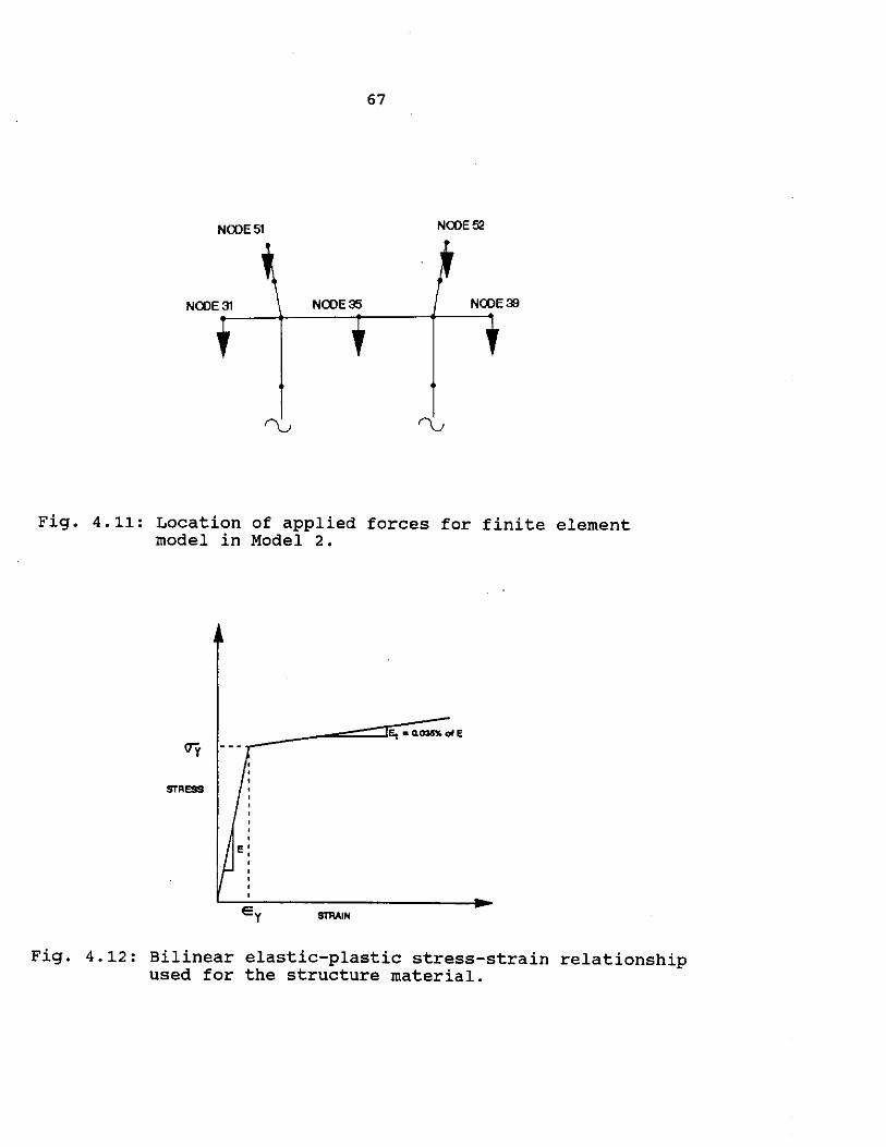
67
NOOE51 NOOE52
NOOE35 NOOE39
Fig. 4.11: Location of applied forces for finite element model in Model 2.
Et • 0.035'4 of E
STRESS
Ey STRAIN
Fig. 4.12: Bilinear elastic-plastic stress-strain relationship used for the structure material.

68
4.3 Development of the Fragility curve
The reliability procedure outlined in Chapter 3 was
applied to an existing transmission line structure by first
analyzing Model 1 under incremental ice loading. This
analysis established the relationship between the ice
thickness on the conductors and the forces induced at nodes
31, 35, 39, 51, and 52 (see Fig. 4.11). These forces were
then used as an input to perform the structural analysis of
Model 2. The analysis was continued and all possible failure
modes such as buckling, plastic collapse and insulator failure
were investigated.
4.3.1 Results of model 1 analysis
Model 1 was loaded in increments of 0.1 in. of ice until
2.0 in. of ice on the conductors was accumulated. The global
components of the forces (see Fig. 4.10) at nodes 31, 35, 39,
51 and 52 were recorded. The results of this analysis are
shown in Table 4.1.
As would be expected, there is a non-linear relationship
between the accumulation of ice and the forces on the
structure. Also, the predominate direction of the resulting
forces is in the vertical in-plane direction (or Fy) due to
the weight of the ice and conductors. These forces, Fy, are
negative because of the defined coordinate system shown in
Fig. 4.10.

69
Table 4.1: Forces at nodes 31, 35, 39, 51 and 52 due to various ice thicknesses on the conductors.
NODES 31, 35, & 39 ICE
THICKNESS Fy(a) pz(b) (in.) (kips) (kips)
o.o -3.19 0.01
0.1 -3.59 0.02
0.2 -4.05 0.03
0.3 -4.58 0.05
0.4 -5.17 0.07
0.5 -5.84 0.09
0.6 -6.56 0.12
0.7 -7.35 0.16
0.8 -8.20 0.21
0.9 -9.12 0.27
1. 0 -10.11 0.34
1.1 -11.16 0.43
1. 2 -12.27 0.53
1. 3 -13.45 0.65
1.4 -14.69 0.79
1.5 -15.99 0.95
1. 6 -17.36 1.13
1. 7 -18.79 1.34
1.8 -20.28 1.58
1.9 -21. 84 1. 84
2.0 -23.45 2.14
(a) Vertical in-plane loading (b) Lateral out-of-plane loading
NODES 51 & 52
Fy(a) Fz (b) (kips) (kips)
-0.35 0.09
-0.43 0.11
-0.53 0.13
-0.67 0.17
-0.84 0.21
-1. 04 0.25
-1. 28 0.30
-1. 54 0.36
-1. 84 0.43
-2.17 0.50
-2.53 0.58
-2.93 0.65
-3.35 0.73
-3.81 0.82
-4.30 0.91
-4.83 1.01
-5.38 1.10
-5.97 1.19
-6.60 1. 28
-7.25 1. 36
-7.94 1.45
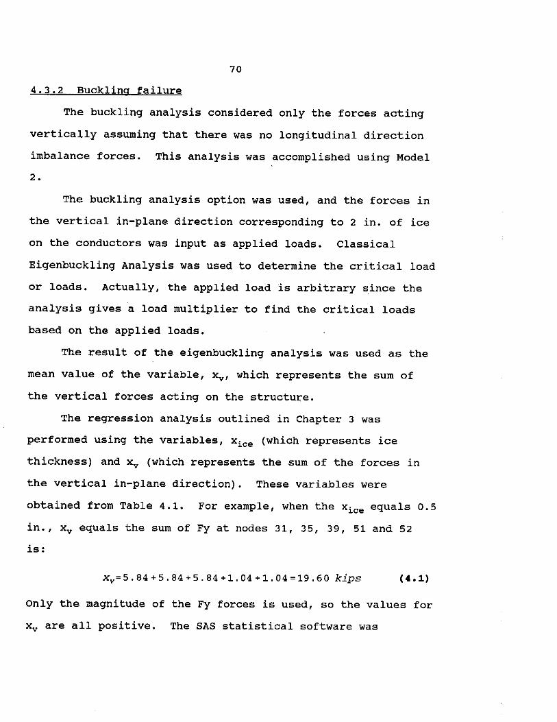
70
4.3.2 Buckling failure
The buckling analysis considered only the forces acting
vertically assuming that there was no longitudinal direction
imbalance forces. This analysis was accomplished using Model
2.
The buckling analysis option was used, and the forces in
the vertical in-plane direction corresponding to 2 in. of ice
on the conductors was input as applied loads. Classical
Eigenbuckling Analysis was used to determine the critical load
or loads. Actually, the applied load is arbitrary since the
analysis gives a load multiplier to find the critical loads
based on the applied loads.
The result of the eigenbuckling analysis was used as the
mean value of the variable, xv, which represents the sum of
the vertical forces acting on the structure.
The regression analysis outlined in Chapter 3 was
performed using the variables, xice (which represents ice
thickness) and xv (which represents the sum of the forces in
the vertical in-plane direction). These variables were
obtained from Table 4.1. For example, when the xice equals 0.5
in., xv equals the sum of Fy at nodes 31, 35, 39, 51 and 52
is:
xv=5. 84 +5. 84 +5. 84 +l. 04 +1. 04 =19 .60 kips (4.1)
Only the magnitude of the Fy forces is used, so the values for
xv are all positive. The SAS statistical software was
71
utilized to perform the analysis and to formulate the failure
function, G8 {x} using the data points which consist of the
variables xice and xv. This analysis yielded the following
failure function:
(4.2)
4 . 3.3 Insulator failure
Failure of any of the three insulators can also be
induced by a heavy ice accumulation on the conductors. The
axial force in the conductors, Xa, i.e., Fy in Table 4.1.
The data points for the regression analysis consisted of
the variables, xice (from the previous failure mode) and xa. A
regression analysis of these data points using SAS was
performed and the resulting failure function for the
insulator, Gr{X}, is:
Gz(x}= 3. 05 + 3. 66 Xice+ 3. 26 xfc9 -Xa (4.3)
This equation represents the failure of a single insulator and
was used to describe all three failures.
Failure of an insulator does not necessarily constitute
failure of the structure, but should be considered as one
possible failure mode.
f
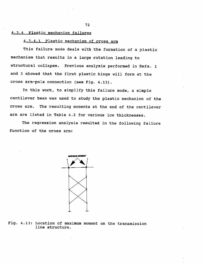
72
4.3.4 Plastic mechanism failures
4.3.4.1 Plastic mechanism of cross arm
This failure mode deals with the formation of a plastic
mechanism that results in a large rotation leading to
structural collapse. Previous analysis performed in Refs. 1
and 3 showed that the first plastic hinge will form at the
cross arm-pole connection (see Fig. 4.13).
In this work, to simplify this failure mode, a simple
cantilever beam was used to study the plastic mechanism of the
cross arm. The resulting moments at the end of the cantilever
arm are listed in Table 4.2 for various ice thicknesses.
The regression analysis resulted in the following failure
function of the cross arm:
Fig. 4.13: Location of maximum moment on the transmission line structure.

73
Table 4.2: Moments at location between the cross-arm and pole.
ICE THICKNESS MOMENT ICE THICKNESS MOMENT (in.) (in*kip) (in.) (in*kip)
o.o 789.48 1.0 2325.1.9
0.1 878.28 1.1 2558.09
0.2 980.39 1.2 2804.25
0.3 1098.04 1. 3 3065.88
0.4 1229.00 1. 4 3340.75
0.5 1.377.70 1.5 3628.82
0.6 1537.50 1. 6 3932.22
0.7 1.712.82 1. 7 4248.1.1.
0.8 1901. 43 1.8 4572.23
0.9 21.05.56
(4.4)
where, Gp{X}= failure equation for the formation of plastic
hinge, = the moment at the connection between the structure
arm and leg.
This limit state equation applies for both left and right
sides of the transmission line structure assuming symmetry.
Therefore, this failure type includes two individual failure
modes, one for the right arm and one for the left arm.
As with the insulator failures, the failure of the cross
arm does not imply failure of the entire structure. However,
one must consider this mode when investigating the failure of
the transmission line structure.

74
4.3.4.2 Plastic collapse of pole
Plastic collapse of the pole may occur when an insulator
or an outboard arm of an adjacent structure fails resulting in
a large imbalance force. This imbalance situation may also
occur when a conductor is broken which as illustrated in Fig.
4.14. The figure depicts a broken middle conductor between
Tower "B" and Tower "C". Such an occurrence is important to
investigate because the resulting imbalance force may yield a
domino pattern of failure.
To investigate this case, Model 2 was analyzed
considering vertical in-plane forces at nodes 31, 35, and 39.
The sum of these forces is referred to hereafter as V. A
horizontal out-of-plane force, H, at node 35 representing an
imbalance force was added to the model. The analysis was
performed four times considering various levels of interaction
between the vertical and horizontal forces. The levels of
interaction between the forces V and H are listed below:
•H = 0.0 v •H = 0.2 v •H = 0.4 v •H = 0.6 v •H = 0.8 v
The first interaction was studied in Section 4.3.2 when
investigating the buckling failure of the structure.
In the structural analysis, these forces were incremented
following the guidelines of the limit analysis procedure in
ETADS, while the induced moments in the poles were monitored.

TOWER "A" TOWER 118 11
TOWER "C"
Fig. 4.14: Force imbalance created at Tower "A" and Tower "C" due to a broken conductor between Tower "B" and Tower "C".
..... CJ1

76
Since the pole is a tapered member, the locations of yielding
was indeterminate and is not at the base of the pole as one
may expect. When full plastic hinges form at these locations,
an unrestricted rotation under any additional load will occur
leading to an unstable structure indicating the loss of the
structure integrity.
Due to symmetry, the formation of a plastic hinge on one
pole of the transmission line corresponds to the formation of
a plastic hinge in the other pole. The failure equations were
developed for· plastic collapse of five pairs of nodes (see
Fig. 4.10), and those pairs are:
• nodes 1 and 2 •· nodes 3 and 4
• nodes 5 and 6
• nodes 7 and 8
• nodes 9 and 10
For convenience, reference to these pairs of nodes will only
include the number of the first node listed.
For interaction level H/V=0.2, the following failure
equations were developed based on the moments obtained from
the structural analyses:
G~.2{x}= -75. 08 -26. 99 V-0. 206x1 *H+x1 (4.5)
(4.6)
G~' 2(x}=-51.43-24. 86 V-0 .20BX5*H+X5 (4.7)
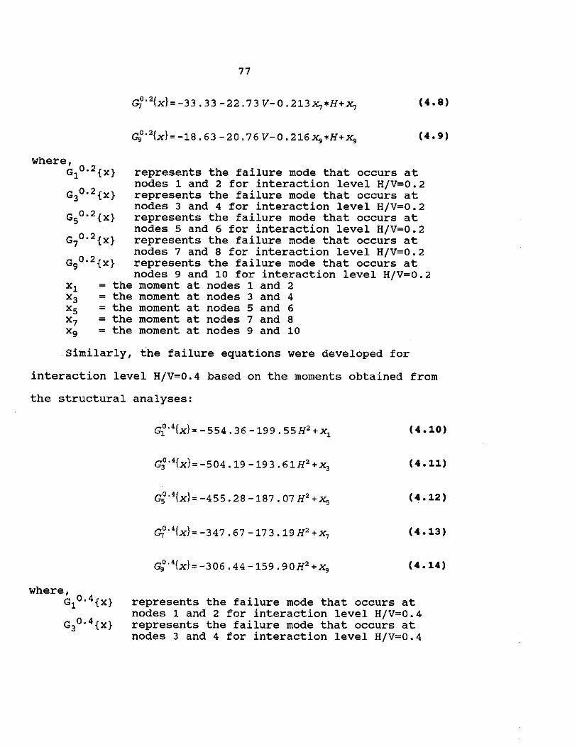
X1 = X3 = X5 = X7 = Xg =
77
try°· 2{x}= -33. 33 -22. 7 3 V- 0. 2l3X,*H+x, (4.8)
G~' 2{x}= -18. 63 -20. 76 V- 0. 216 X,,*H+x,, (4.9)
represents the failure mode that occurs at nodes 1 and 2 for interaction level H/V=0.2 represents the failure mode that occurs at nodes 3 and 4 for interaction level H/V=0.2 represents the failure mode that occurs at nodes 5 and 6 for interaction level H/V=0.2 represents the failure mode that occurs at nodes 7 and 8 for interaction level H/V=0.2 represents the failure mode that occurs at nodes 9 and 10 for interaction level H/V=0.2
the moment at nodes 1 and 2 the moment at nodes 3 and 4 the moment at nodes 5 and 6 the moment at nodes 7 and 8 the moment at nodes 9 and 10
Similarly, the failure equations were developed for
interaction level H/V=0.4 based on the moments obtained from
the structural analyses:
where, Gl 0.4{x}
G30.4{x}
(4.10)
G~' 4{x}= -504 .19 -193. 61H2 +x3 (4.11)
Gi·•{x}= -455. 28 -187. 07 H 2 +x5 (4.12)
c,0 •4{x}= -347. 67 -173 .19 H 2 +x, (4.13)
Gr•1xl= -306. 44 -159. 90H2 +x,, (4.14)
represents the failure mode that occurs at nodes 1 and 2 for interaction level H/V=0.4 represents the failure mode that occurs at nodes 3 and 4 for interaction level H/V=0.4

Gs0.4{x}
G10.4{x}
Gg0.4{x}
78
represents the failure mode that occurs at nodes 5 and 6 for interaction level H/V=0.4 represents the failure mode that occurs at nodes 7 and 8 for interaction level H/V=0.4 represents the failure mode that occurs at nodes 9 and 10 for interaction level H/V=0.4
For interaction level H/V=0.6, the failure equations were
developed and are listed below:
where, G10.6{x}
G30.6{X}
Gs0.6{X}
G70.6{X}
Gg0.6{x}
( 4. 15)
Gf ' 6 (x}= -727. 63 -132, 39 H 2 +x3 (4.16)
Gi' 6{x)= -664. 72-127. 43H2 +Xs (4.17)
~o · 6{x) = -56 O . 4 O - 11 7 . 14 H 2 + x., ( 4. 18)
Gr 6lxl= -411. 08 -101. 45 H 2 +x. ( 4. 19)
represents the failure mode that occurs at nodes 1 and 2 for interaction level H/V=0.6 represents the failure mode that occurs at nodes 3 and 4 for interaction level H/V=0.6 represents the failure mode that occurs at nodes 5 and 6 for interaction level H/V=0.6 represents the failure mode that occurs at nodes 7 and 8 for interaction level H/V=0.6 represents the failure mode that occurs at nodes 9 and 10 for interaction level H/V=0.6
Lastly, the failure equations for interaction level
H/V=0.8 were developed and are listed below:
G~' 8{x)= -1025. 35 -105. 05H2 +X1 (4.20)
Gf ' 8{x)= -951. 63 -101. 04H2 +x3 (4.21)
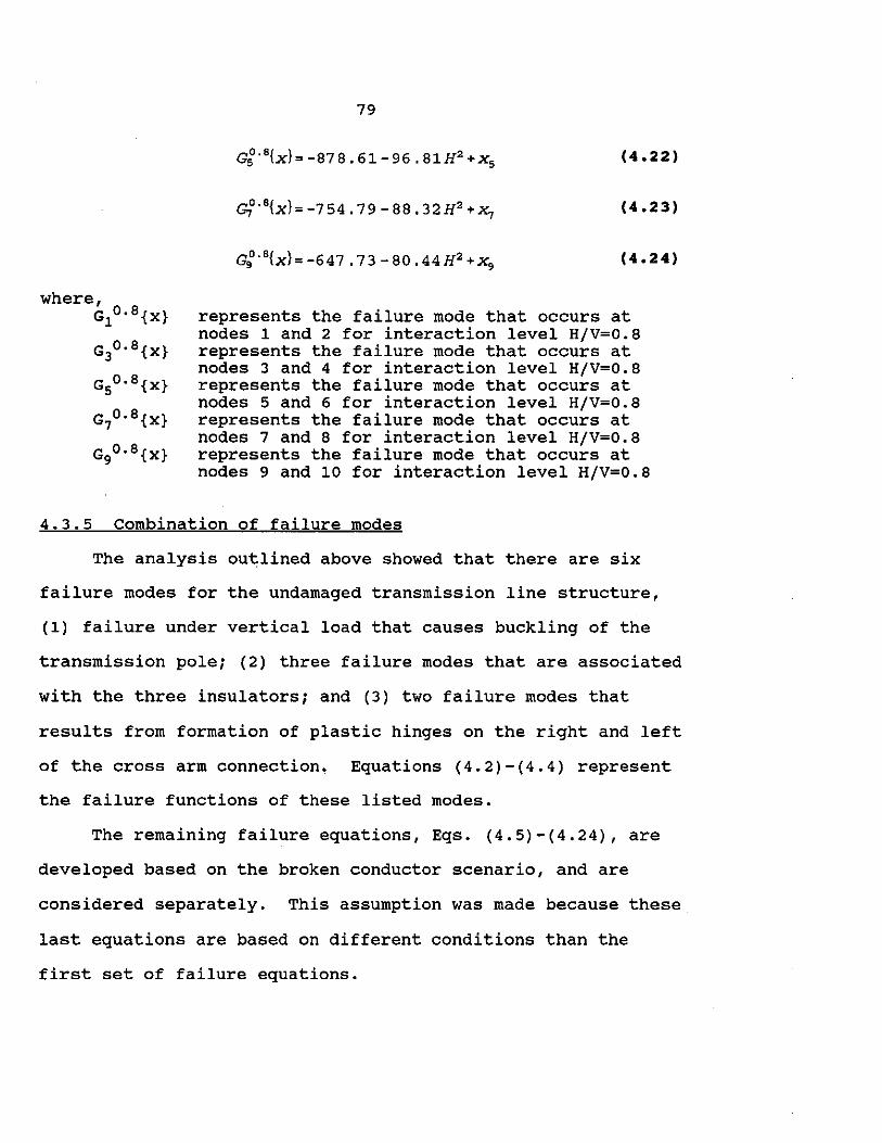
where, Gio.a{x}
G30.8{X}
Gso.a{x}
G10.a{x}
Ggo.a{x}
79
G~' 8{x}= -87 8. 61-96. 81H2 +x5 (4.22)
~· 8{x}= -754. 79 -88, 32H2 +x, (4.23)
Gr"lxl= -647. 13 -00. 44H2 +"'9 (4.24)
represents the failure mode that occurs at nodes 1 and 2 for interaction level H/V=0.8 represents the failure mode that occurs at nodes 3 and 4 for interaction level H/V=0.8 represents the failure mode that occurs at nodes 5 and 6 for interaction level H/V=0.8 represents the failure mode that occurs at nodes 7 and 8 for interaction level H/V=0.8 represents the failure mode that occurs at nodes 9 and 10 for interaction level H/V=0.8
4.3.5 Combination of failure modes
The analysis outlined above showed that there are six
failure modes for the undamaged transmission line structure,
(1) failure under vertical load that causes buckling of the
transmission pole; (2) three failure modes that are associated
with the three insulators; and (3) two failure modes that
results from formation of plastic hinges on the right and left
of the cross arm connection, Equations (4.2)-(4.4) represent
the failure functions of these listed modes.
The remaining failure equations, Eqs. (4.5)-(4.24), are
developed based on the broken conductor scenario, and are
considered separately. This assumption was made because these
last equations are based on different conditions than the
first set of failure equations.
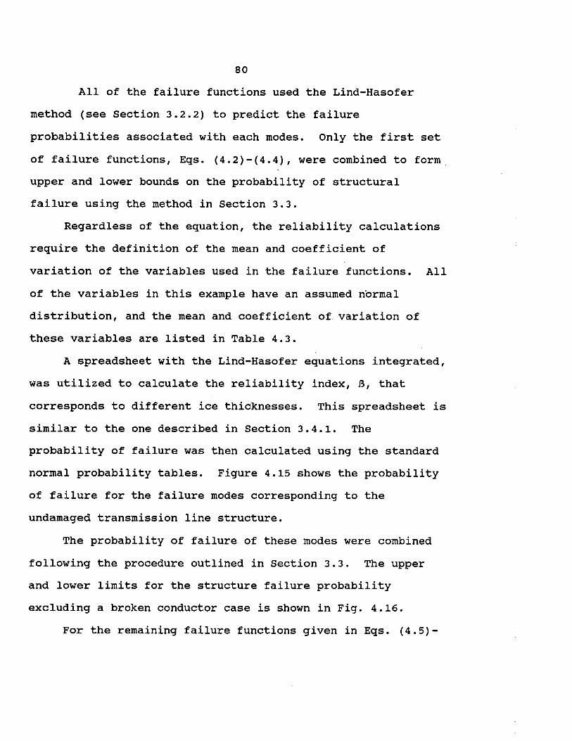
80
All of the failure functions used the Lind-Hasofer
method (see Section 3.2.2) to predict the failure
probabilities associated with each modes. Only the first set
of failure functions, Eqs. (4.2)-(4.4), were combined to form
upper and lower bounds on the probability of structural
failure using the method in Section 3.3.
Regardless of the equation, the reliability calculations
require the definition of the mean and coefficient of
variation of the variables used in the failure functions. All
of the variables in this example have an assumed normal
distribution, and the mean and coefficient of variation of
these variables are listed in Table 4.3.
A spreadsheet with the Lind-Hasofer equations integrated,
was utilized to calculate the reliability index, B, that
corresponds to different ice thicknesses. This spreadsheet is
similar to the one described in Section 3.4.1. The
probability of failure was then calculated using the standard
normal probability tables. Figure 4.15 shows the probability
of failure for the failure modes corresponding to the
undamaged transmission line structure.
The probability of failure of these modes were combined
following the procedure outlined in Section 3.3. The upper
and lower limits for the structure failure probability
excluding a broken conductor case is shown in Fig. 4.16.
For the remaining failure functions given in Eqs. (4.5)-

81
Table 4.3: variables with mean values and coefficient of
If! 3 LE u. 0 ~ :::J
'° cs ~ a..
variation (COV).
Variable
X.;--
H
x,.
x.
lL
x,
X1
x~
X7
Xq
1E+OO
1 E..Q<I
1E..08
,'
1E·12 ,'
Mean
(variable)
(variable)
80 kips
18 kips
4,578 in*kips
10,618 in*kips
10,106 in*kips
7,025 in*kips
6,337 in*kips
5,735 in*kips
--- ---,"~.····
,' - . ,' , .··
' .· ' . ',, ......
' .. ,' ... Insulator Failure
Plasti!l_~9\lapse
Buckling failure
cov
0.10
0.10
0.05
0.05
0.05
0.05
0.05
0.05
0.05
0.05
1E·18 ....__.___,_-'---'--'--~~~~~-~~_,_-'-__,__.___.___,_-'-__,_-~ 0.0 0.2 0.4 o.e 0.8 1.0 1.2 1.4
ICE THICKNESS (In.) 1.8 1.8 2.0
Fig. 4.15: Probability of failure curves for individual failure modes for undamaged transmission line structure.
2.2
1E+OO
w c:: ::J 1E..Q4 ...J
Lt LL. 0 ~ 1E..Q8
::J ffi 05
1E·12 ~ a.
. . :
. . . . . .
82
,,
---------- ------------------
UPPERBOUNO
LOWl;fl_ ~9U N 0
1 E· 1 S ""--'--'--'----'-'---'--'--'---'-___.-..___,__._-'-__..-'---'--'--'----'-,___, 0.0 0.2 0.4 o.s 0.8 1.0 1.2 1.4
ICE THICKNESS (In.) 1.8 1.8 2.0
Fig. 4.16: Fragility curve with upper and lower bounds for undamaged transmission line structure.
2.2
(4.24), the same procedure was followed except that no
combination of the failure probabilities was considered. Since
these equations do not pertain to the same loading conditions,
these equations cannot be combined to form an
overall structural probability of failure. However, the
probability of failure for the individual failure modes were
found. Figure 4.17 shows the five probability of failure
curves for interaction level, H/V=0.20, and Fig. 4.18 shows
those probability of failure curves for interaction level,
H/V=0.4. Figures 4.19 and 4.20 display the probability of
failure curves for interaction levels, H/V=0.6 and H/V=0.8
respectively. Figure 4.21 depicts the dominate failure mode

1E+oo
UJ 1E-01
a: 3 1E-02
~ ~ 1E-03
~ 1E-04 ::J
CD d5 ~
1E-Oe
0. 1E-Oe
1E-07 3.0
83 HIV= 20%
4.0 4.8
VERTICAL FORCE (kips)
NODEI , 3 5 7 9
(eee Fig, 4, 10)
Fig. 4.17: Probability of failure curves for individual failure modes for broken insulator case where the interaction level is H/V=0.2.
1E+oo
UJ 1E-01
a: 3 1E-02
~ ~ 1E-03
~ ::J 1E-04
CD d5 ~
1E-Oe
0. 1E-Oll
1E-07 4.4
H/V=40%
4.0 4.B e.o e.a 8.4
VERTICAL FORCE (kips)
NODEI , 3 5 7 g
(eee Fig. 4, 1 0)
e.e 8.B e.o
Fig. 4.18: Probability of failure curves for individual failure modes for broken insulator case where the interaction level is H/V=0.4.

1E-02
1E-03 •• =--" ,"'
1E-04
.. ·· 1E-Oe
84 V/H = 80%
,,,,. .. ·
NOCEI 1 3 5 7 9
(eee Fig. 4. 10)
1E-Oel-~-'-~.....L..~-'-~___.~~'--~-'-~_.__~_._~__._~~~~~~~
U M ~ M M U M
VERTICAL FORCE (kips)
Fig. 4.19: Probability of failure curves for individual failure modes for broken insulator case where the interaction level is H/V=0.6.
1E+oo
w c:: tE-01
:::> ..J
~ t E-02
~ 1E-03
~ ::J 1E-04
~ ~
1E-Oe
a. 1E-Oe
tE-07 e.4 e.e
HN= 80%
7.0 7.2 7.4 1.e VERTICAL FORCE (kips)
NOO:: I 1 3 5 7 9
(see Fig, 4.10)
7.8 8.0
Fig. 4 . 20: Probability of failure curves for individual failure modes for broken insulator case where the interaction level is H/V=0.8.

/. / .... ·
/.-·· / .....
, ,
85
H/V NODE# 20% 9 40% 5 80% , 90% 3
(see Fig. 4. 1 0)
1E-Oe'--~~~--'-~~~-'-~~~~'--~~~-'-~~~-'-~~~~ Q.e 3.0 3.e 4.0 4.e
VERTICAL FORCE (kips)
Fig. 4.21: Probability of failure curves for the dominate failure modes of the four interaction levels.
Of each interaction level which are:
1. For interaction level, H/V=0.2, the plastic collapse of nodes 9 and 10.
2. For interaction level, H/V=0.4, the plastic collapse of nodes 5 and 6.
3. For interaction level, H/V=0.6, the plastic collapse of nodes 1 and 2.
4. For interaction level, H/V=0.8, the plastic collapse of nodes 3 and 4.
4.3.6 Interpretation of fragility curves
The fragility curve for the undamaged transmission line
structure, shown in Fig. 4.16, represents the probability of
failure for a given ice thickness. The ice storms in Mid-
Iowa, which resulted in the previous studies, produced an
approximate ice thickness of 1.25 to 1.5 in. of ice

86
accumulation on the conductors. For 1.25 in. of ice, the
probability of structural failure is 15%-45% based on the
calculations made in this study. For 1.5 in. of ice, the
probability increases to the range of 35%-85%. In this case,
failure most likely will result from buckling of the line.
This is true if and only if no broken insulator or conductor
occurs.
The probabilities of failure for the ice thicknesses of
1.25 in. and 1.5 in. indicate that there is high chance that
the transmission line structure would be structural damaged
during an ice storm which produced this amount of ice. Based
on this information, one might say that the structure needs to
be strengthened. But if the ice storm only occurs once every
so-years, then strengthening this structure may not be an
economically wise decision. The fact that two of these ice
storms occurred in Iowa within a span of 18 months does not
indicate that these storms are typical of this area. There is
a trade-off between the goal to prevent any failure and the
cost of such a venture.
Alternatively, Fig. 4.21 can be used to interpret the
probability of failure for a given ice thickness; however, the
probability of failure is not interpreted the same as the
previous case. The resulting probability is the failure
probability of a damaged transmission line structure, such as
one with a broken conductor or insulator.

87
To exemplify this case, consider an ice thickness of 0.5
in. The sum of the vertical forces is 19.6 kips (see Table
4.1). Assuming an interaction level between the horizontal
force and the vertical force as H/V=0.2, the horizontal force
is 3.9 kips. This corresponds to a probability of failure of
approximately 5.0%. But the chance of the transmission line
structure having a broken conductor at 0.5 in. of ice is
negligible.
If the ice thickness was 1.25 in., which has a
significant probability of the structure resulting in a broken
conductor, the sum of the vertical forces is 46.0 kips. Again
assuming the same interaction· level (H/V=0.2), the horizontal
force is 9.2 kips. Based on the calculations in this work,
this force corresponds to a probability of failure of almost
100%. Realistically, this means that once the ice loads
results in breaking a conductor, the probability of structural
failure would be significant.
Engineering economic analysis using these probability of
failure curves, Fig. 4.16 and Fig. 4.21, would provide
engineers with more data with which to evaluate the condition
of the transmission line structure under consideration. An
engineering economic analysis may be accomplished using
methods described in Ref. 23.

88
S. SUMMARY AND CONCLUSIONS
s.1 summary
The occurrence of two major ice storms in Mid-Iowa
resulted in the damage and collapse of many transmission line
structures. The first happened on March 7, 1990 and caused 68
failed structures. On October 31, 1991, the second storm hit
Iowa and caused the most destruction in Iowa's history. These
events were previously investigated and analyzed by others to
determine possible failure scenarios. The first ice storm
analysis suggested that a probabilistic analysis needed to be
performed.
The design of transmission line structures typically does
not encompass probabilistic theory or reliability concepts
such as Load and Resistance Factor Design (LRFD) that has been
recently adopted in design of steel buildings. However, some
reliability based design methods for transmission lines have
been developed; two methods were proposed by the American
Society of civil Engineers and International Electrotechnical
Commission. As designers use these procedures, the acceptance
of reliability based design for transmission line structures
should continue to grow.
Meanwhile, the methods followed to perform a
probabilistic analysis of existing transmission line
structures are varied. The development of the required limit
state functions for these procedures require knowledge of

89
closed form solutions which involves rigorous manipulations of
equations for a transmission line structure. The reliability
analysis procedure developed in this study does not require
this knowledge.
The limit state function needed to perform a reliability
analysis was developed herein using a regression analysis.
Once the limit state function was established, the Lind-
Hasofer FOSM method was used to analyze the limit state
function and to estimate the probability of failure associated
with the various failure modes and corresponds to different
load levels. These probabilities were then used to construct
fragility curves for the system failure probability.
In this study, the load was the accumulation of ice on
the conductors and shield wires. Four basic types of failures
of the transmission line structure were investigated:
• buckling of the structure poles, • failure of the insulators, and • formation of a plastic hinge at the connection point
between the outboard arm and pole. • failure of the transmission line structure subjected to
unbalanced forces due to a broken conductor buckling of the structure poles.
Specifically, the last type of failure of the
transmission line structure dealt with a broken central
conductor. This condition resulted in the formation of
plastic hinges in the poles of the transmission line
structure.

90
5.2 conclusions
The resulting fragility curves provide information about
the existing transmission line structure. This information
can be use to determine the condition of a structure under
different loadings. The condition of a structure is
interpreted by the probability of failure.
The probability of structural failure was determined for
an ice thickness on the conductors of 1.5 in. to be between
35% and 85%. After the ice storm in Mid-Iowa on March 7,
1990, the amount of ice on the conductors was recorded as
1. 25-1. 50 in. The analysis of the transmission line involved
in this ice storm determined that critical load of the
structure happened when the ice thickness was between 1.50 and
1.75 in. of ice (1). Based on this information, one might say
that the structure needs to be strengthened. But if the ice
storm only occurs once every 50-years, then strengthening this
structure may not be an economically wise decision.
Interpretation of the probability of failure data should be
compared with the frequency of the loading in order to make
judgements about the condition of a structure. There is a
trade-off between the goal to prevent any failure and the cost
of such a venture.
5.3 Recommendations for Further Research
The probabilistic analysis procedure presented in this
study may be further investigated to include different

91
applications, more variables, the variability of more
parameters and the uncertainty of the variables.
Many other scenarios may be considered using this
probabilistic analysis procedure, including different loading
conditions, combinations of various loading conditions, and
different types of transmission line structures. Various
climatic conditions such as wind and the combination of wind
and ice accumulation are possible scenarios.
Some variables to incorporate into the analysis are the
difference of adjacent span lengths between transmission line
structures and the angle between structures.
The parameters which were included in this work are ice
thickness, plastic moment capacities of joints in the
structure, and strength of the insulators. These parameters
could be separated so that the geometric dimensions of the
structure and material properties associated with the
parameters could be included in the analysis. The inclusion
of the geometric dimensions and material properties would
increase the computations and structural analysis runs
significantly, but the benefit would be the inclusion of the
variability of these parameters in the analysis. Sensitivity
studies would indicate which parameters have the most effect
on the probability of failure.

1. s. Gupta. structures 1991.
92
REFERENCES
"Nonlinear Analysis of Transmission Line Subjected to Ice Loads." Thesis, Iowa State u,
2. "Electric Power Research Institute's TLWorkstation software, module ETADS." Palo Alto, CA, July 1990.
3. A. Nafie. "Failure Analysis of Transmission Line Structures." Thesis, Iowa State U, 1993.
4. H. J. Hillarker. "Preliminary monthly weather summary -November 1991. 11 State Climatologist's report, Iowa Department of Agriculture and Land Stewardship, Des Moines, IA.
5. Y. Ibrahim. "General Strategy for Structural Systems Reliability Analysis." Journal of Structural Engineering vol. 114 (March 1991): 789-807.
6. H. o. Madsen, s. Krenk and N.C. Lind. Methods of Structural Safety. Englewood Cliffs, NJ: Prentice-Hall, 1986.
7. L. Griemann and W. Knapp. Reliability Assessment for the Buckling of Stiffened Cylinders. Final Report submitted to Conoco, Inc.,ISU-ERI-Ames-83284, ERI Project-1564. Engineering Research Institute, Iowa State U, June 1983.
8. P. Thoft-Christensen and Y. Murotsu. Application of Structural Systems Reliability Theory. Berlin, Heidelberg: Springer-Verlag, 1986.
9. SAS Institute Inc. SAS User's Guide: Statistics, Version 5 Edition. Cary, NC: SAS Institute Inc., 1985.
10. National Electrical Safety Code. National Bureau of Standards. Washington, DC: U.S. Govt. Print. Off., 1989.
11. A. Peyrot, M. Maamouri, H. Dagher and s. Kulendran. "Reliability-Based Design of Transmission Lines: A Comparison of the ASCE and IEC methods." Third International Conference on Probabilistic Methods Applied to Electric Power Systems. London: Institute of Electrical Engineering, 1991.
12. ASCE Guidelines for Transmission Line Structural Loading. New York, NY: American Society of Civil Engineers, 1991.
93
13. IEC Technical Committee No. 11, Loading and Strength of Overhead Transmission Lines, 1988 draft, International Electrotechnical Commission, Geneva, Switzerland.
14. F. G. Picciano. "The NESC, Probability, Reliability and the Future." Probabilistic Methods Applied to Electric Power Systems, Proceeding of the First International Symposium, Toronto, Canada. 11-13 July, 1986. New York, NY: Pergamon Press, 1987.
15. H. J, Dagher, s. Kulendran, A. H. Peyrot and M. Maamouri. "System Reliability Concepts in the Design of Transmission Lines." National Science Foundation MSM-8821079, EPRIRP1352-ll. Final Report, 1992.
16. A. Kamarudin. "A Censoring Technique in the Monte Carlo Simulation Method Applied to Probability Based Distribution Line Wood Pole Design." Probabilistic Methods Applied to Electric Power systems, Proceeding of the First International Symposium, Toronto, Canada. 11-13 July, 1986. New York, NY: Pergamon Press, 1987.
17. A. K. Haldar. "Structural Reliability Analysis of a Transmission Tower using Probabilistic Finite Element Method." Probabilistic Methods Applied to Electric Power Systems, Proceeding of the First International Symposium, Toronto, Canada. 11-13 July, 1986. New York, NY: Pergamon Press, 1987.
18. Y. Murotsu, H. Okada, s. Matsuzaki and s. Nakamura. "On the Probabilistic Collapse Analysis of Transmission Line Structures." Probabilistic Methods Applied to Electric Power Systems, Proceeding of the First International Symposium, Toronto, Canada. 11-13 July, 1986. New York, NY: Pergamon Press, 1987.
19. A. Haldar. "Recent Failure of a Transmission Line due to Ice in Newfoundland." Fifth International Workshop on Atmospheric Icing of Structures. Tokyo, Japan: Arcadia Ichigaya, 1990.
20. "Tables of the Bivariate Normal Distribution Function and Related Functions." U.S. Department of Commerce, National Bureau of Standards, Applied Mathematics Series, 50. Washington, DC: U.S. Govt. Print. Off., 1953.
21. T. A. Ryan. Minitab Reference Manual. Ames, Iowa: Computation Center, Iowa State u, 1981.
22. M. Gorman and F. Moses. "Direct Estimate of Structural

94
System Reliability," seventh Conference on Electronic Computation. New York, NY: American Society of Civil Engineering, 1979.
23. s. K. Adams. Engineering Economic Analysis. New York, NY: McGraw-Hill, 1991.

95
ACKNOWLEDGEMENTS
I would like to thank my co-major professors, Dr. Fouad
Fanous and Dr. Terry Wipf, for all of their support and
guidance in my research. Fouad Fanous was especially
understanding and helpful.
Most of all, I extend my deepest thanks to my husband,
Bob, for everything that he has done to make it possible for
me to complete my research.