probabilistic design of structures submitted to fatigue · chapter 5 probabilistic design of...
TRANSCRIPT

Chapter 5
Probabilistic Design of Structures Submitted toFatigue
5.1. Introduction
The fatigue behavior of materials submitted to cyclic loading is a randomphenomenon at any scale of description. When considering materials withoutmicroscopic defects, the fatigue initiation sites usually correspond to the creation ofslip bands within the superficial grains and are influenced by the size and the locationof the grains as well as the roughness of the material surface. When consideringmaterials with inclusions (e.g. carbides within nickel-based alloys) or defects (micro-cavities in cast steels), the latter may become preferential sites for crack initiation.The location and the size of these defects within an elementary material volume arenaturally random ([BAT 10], Chapter 3).
Once the crack has been initiated at the microscopic scale, its trans-granularpropagation in stage I is controlled by the crystalline orientation of the grain and itsneighbors: the fine description of this phenomenon can be deterministically modeledat the grain scale. Nevertheless, when considering the crack propagation at themacroscopic scale of the structure, the phenomenon is still random.
At the specimen scale, the different mechanisms that are presented above, cannotbe predicted: deterministically the lifetime of a specimen of a particular material(i.e. whose composition is perfectly controlled) subjected to an identical loading,varies from one specimen to another: this is the distribution observed by any
Chapter written by Bruno SUDRET.

236 Fatigue of Materials and Structures
experimenter, and which can be represented by a scatter plot within the (logN, S)plane, where S is the loading amplitude and N the number of cycles to failuremeasured according to the standards, e.g. [AFN 90].
If the fatigue phenomenon is considered through the propagation of a crack undera cyclic loading at the macroscopic scale, it is usually observed that the parameterscontrolling the propagation (e.g. Paris law’s parameters [PAR 63]) are random, asshown, for instance in [VIR 78] for aluminum.
Thus the random aspect of the fatigue phenomenon seems to be occurring at allscales of description. However, if we pay a close attention to the regulations in forceregarding the behavior of loaded structures under fatigue conditions, they are based ondeterministic rules (RCC-M code for the nuclear industry [AFC 00], AC25.571-1rules of the Federal Aviation Administration for the space industry, etc.). Relyingon so-called conservative criteria (which means that the design performed accordingto these criteria shall ensure safety by construction), they are based on simplifiedengineering models. In addition, academic work on fatigue often tends to explaindeterministically how the fatigue phenomena occur.
From these initial observations, it seems important to develop a coherentprobabilistic fatigue phenomenon approach based on a fine description of the physicsat the desired scale and on a rigorous treatment of uncertainty. For the last tenyears, the uncertainty treatment in physical models has been studied in variousprobabilistic engineering mechanics (reliability of the structures, domains, stochasticfinite elements). It is therefore suitable to apply the general uncertainty quantificationmethods to the fatigue problems of materials and structures: this is what this chapterfocuses on.
A general framework dealing with the treatment of the uncertainties in mechanicalmodels is proposed in section 5.2. Different statistical treatment methods of fatiguedata are then described in section 5.3. A probabilistic design methodology is thenproposed in section 5.4. The uncertainty issue regarding the propagation of existingcracks is addressed in section 5.5, by considering some non-destructive test data toupdate the predictions.
5.2. Treatment of hazard in mechanical models
5.2.1. General scheme
The treatment of uncertainties in mechanical models has been studied for thepast 30 years and took different names such as random mechanics [KRE 83],structural reliability [DIT 96, LEM 05, MEL 99], stochastic finite elements [GHA 91]or sensitivity analysis [SAL 00, SAL 04] depending on the research area. Under these

Probabilistic Design of Structures Submitted to Fatigue 237
different names, we can find a common methodology which allow us to come up withFigure 5.1 [SUD 07].
Figure 5.1. Uncertainty treatment in mechanical models
In the first step (called A), we usually define the model of the consideredmechanical system, and especially its input parameters and its response (also namedquantity of interest). We shall call x the vector of the input parameters, whichmay describe the geometry of the system (length of the elements, shape of thecross-sections, etc.), the behavior (elasticity moduli, parameters of the constitutivelaws) and the applied loading. The response y = M(x) is usually a vectorgathering displacements, stress and strain components, internal variables (strainhardening, damage indicators), etc. It may also contain some post-processedquantities (e.g. amplitudes of extracted cycles by the Rainflow method, cumulativedamage, etc.). Criteria related to these quantities of interest are also usually defined(e.g. acceptable threshold for a specific response in the context of reliability analysis).
5.2.2. Probabilistic model of the input parameters
As the model and its input parameters have been defined, we shall now focus onthose parameters that are uncertain and define a probabilistic modeling. The sourcesof uncertainty, which can be multiple, are usually split into two categories:
– The epistemic uncertainties, which are due to a lack of knowledge (e.g. lack ofprecision of the measurements, lack of data which may lead to insufficient reliablestatistical sampling, etc.). They can usually be reduced in a sense since an acquisitionof additional data or more precise data allows us to decrease their number.
– The random uncertainties, which are intrinsic with respect to the observedparameter, and cannot be reduced. This is typically the case for the quantity “number
238 Fatigue of Materials and Structures
of cycles to failure of a material under cyclic loading with a given amplitude”: themore specimens are tested in the same experimental conditions, the more likely it isto find some extreme values of this number of cycles (low or high). This randomuncertainty can also show a spatial variability as is the case for the properties ofgeomaterials.
Building a probabilistic model of the parameters (step B) consists of definingthe probability distribution function (PDF) of the random vector X of the inputparameters. When we do not have enough data to model the variability of a parameter,we can rely on expert judgment: we assume a certain shape of the distribution of theconsidered parameter (e.g. Gaussian distribution, uniform, lognormal, Weibull, etc.)and then we set up the mean value and the standard deviation of the distribution. Todo so, guidelines are available in [JOI 02].
When data is available, we may use common statistical inference techniques[SAP 06]. In general, we search for the best distribution among selected families(for instance, using the maximum likelihood method) and then carry out goodness-of-fit tests to validate or discard the different choices. For fatigue issues, this typeof statistical analysis is performed to process test data in order to establish theprobabilistic Wöhler curves, as we will see in section 5.3. When the availablesample set has a small size, we may combine the data with some prior informationon the distribution (that represents expert judgment) by using Bayesian statistics[ROB 92, DRO 04].
Sometimes, the variability of the parameters of interest cannot be directlymeasured (e.g. parameters of the model of crack initiation), but this variability canbe apprehended through the measurements of quantities of interest which dependon it (e.g. number of cycles to failure). In these cases we have to rely onprobabilistic reverse methods. Broadly speaking these inverse problems are unsolvedyet. Some recent studies have recently been published in the field of fatigue though[PER 08, SCH 07]. Whatever the selected approach, step B eventually yields aprobabilistic description of the input data as the probability density function fX(x)of the random vector of the input parameters X (see Appendix A for the elementarynotions of probability).
5.2.3. Uncertainty propagation methods
Once both the mechanical model and the probabilistic model of its inputparameters have been established, we shall focus on the propagation of uncertainty

Probabilistic Design of Structures Submitted to Fatigue 239
(step C in Figure 5.1). We are now ready to characterize the random response of themodel, written as Y = M(X)1.
Figure 5.2. Classification of the methods of uncertainty propagation
Depending on what information we are looking for on Y (which is assumed tobe a scalar quantity in this chapter for the sake of simplicity), we usually distinguishdifferent types of analyses (Figure 5.2):
– Analysis of the central tendency, where we mainly focus on the mean value µY
and on the variance σ2Y of the quantity of interest Y (higher order statistical moments
may also be computed). If the distribution of the response Y was Gaussian, thesetwo scalars would completely characterize it. However, this assumption is usuallywrong in practice: thus the statistical moments shall be used for what they are, withoutdeducing any information on the distribution of Y from their values.
– Reliability analysis, where we focus on the probability that the response is abovea certain threshold y. We then have to estimate the tail of the distribution of Y in thiscase. The associated probability (called failure probability) is usually low, with valuesranging from 10−2 to 10−8.
– Distribution analysis, where we are looking to characterize the probabilitydensity function of Y completely.
Specific methods have been proposed for every type of problem, which are givenbelow. For more information, refer to [SUD 07]:
– The Monte Carlo method is the best known method of uncertainty propagation[RUB 81]. It allows us to resolve the problems presented above at least theoretically.
1. If the variability of some parameters of the model is equal to zero or is negligible, we canconsider them as deterministic and gather them within a vector d, and we shall write Y =M(X,d).

240 Fatigue of Materials and Structures
It relies on the simulation of random numbers by specific algorithms which generatea sample set of input parameters conforming to the probabilistic model built in stepB (i.e. according to the distribution fX ). In general, this method is quite efficientfor the calculation of the first statistical moments mean value and variance but getscomputationally expensive when considering reliability or distribution analysis.
– The perturbation method, which was developed in mechanics in the 1980s, relieson a Taylor series expansion of model M around the nominal value of parameters x0
and allows the mean value and standard deviation of the quantities of interest to beefficiently estimated. The gradients of model M with respect to the input parametersneed to be calculated. This method is nowadays used efficiently when these gradientsare directly implemented into the finite element codes used in industrial application(e.g. Code_Aster [EDF 06]).
– The resolution of reliability problems, i.e. the estimation of the probability offailure historically led to some specific methods back in the 1970s. The FORM/SORMmethods (respectively first and second order reliability method) were established inthe 1980s and have been used by some industries (offshore, nuclear industry) for about15 years. They are approximation methods of the distribution tail of the response anddo not allow us to estimate the quality of the obtained result. They are usually coupledto some advanced simulation methods (directional simulation, importance sampling,subset simulation, etc.) [LEM 09].
– Initially introduced in the spectral stochastic finite elements method [GHA 91],representations of response Y by polynominal chaos are nowadays a promisingapproach for the treatment of uncertainties. The principle is to consider therandom response Y within a suitable functional space of random variables, inwhich a foundation is built. Response Y is then completely represented throughits “coordinates” in this basis, which are the coefficients of the polynominal chaosexpansion. These coefficients may be calculated by some non-intrusive methodsfrom a limited number of model evaluations, namely Y = y(i) = M(x(i)), i =1, . . . , N. The analytical post-processing of the coefficients provides the distributionof Y at no additional calculation costs as well as its statistical moments, theprobabilities of exceeding a threshold, etc. [SUD 07].
– Most of the methods of uncertainty propagation give, as by-products (withalmost no additional calculation), some information on the relative significance ofthe input parameters of the model: we call these by-products importance factor orsensitivity indices depending on the methods. This hierarchization (or ranking) of theparameters according to their importance is called “step C” in Figure 5.1.
5.2.4. Conclusion
In this introductory part, we tried to focus on defining a general frameworkfor dialing with uncertainties in mechanical models. We defined of the differentnecessary ingredients and then presented the most commonly used calculation

Probabilistic Design of Structures Submitted to Fatigue 241
methods. The general scheme will now be applied to different problems related tothe fatigue of materials and structures.
5.3. Plotting probabilistic S–N curves
5.3.1. Introduction
The experimental points obtained from fatigue testing are usually plotted in the“amplitude S/number of cycles to failure N” space in order to get the so-called Wöhlercurves ([BAT 10], Chapter 2). In France, the statistical treatment obeys a standard[AFN 91] (mainly inspired by the work of Bastenaire [BAS 60]), which providesmethods to obtain the endurance limit using the staircase method (Section 5 of thestandard), the median Wöhler curve (Section 6), or some probabilistic S −N curves(ESOPE method, Section 9).
The latter is summarized below in Section 5.3.2. A global approach forestablishing probabilistic S − N curves is proposed. This approach is based on thestudies performed independently by Guédé [GUÉ 05], Perrin [PER 08], and Pascualand Meeker [PAS 97, PAS 99]. It has recently been used in industry by EDF andEADS [SCH 06, SCH 07].
Regardless of the approach, we consider a sample set of measurements:
E = (Si, Ni), i = 1, . . . , Q [5.1]
where Ni is the number of cycles to failure measured under alternate stress ofamplitude Si and Q is the size of the sample set. We consider that the sample setcontains test results carried out in the same experimental conditions, allowing one totreat all the experimental points as a whole. We will also consider the data obtainedin the case when the fatigue test has been stopped before failure has occurred. Thisso-called censored data is denoted by N∗
i .
5.3.2. ESOPE method
The ESOPE method, recommended by the AFNOR standard (A 03-405, Section 8)[AFN 91] is based on the following assumption: within a sample E as presented above,we suppose that the fraction F (S,N) of the specimens, which failed before N cyclesof amplitude S, has the following particular form:
F (S,N) = Φ
(S − µ(N)
σ
)[5.2]
where σ is a distribution parameter, Φ is the standard normal (Gaussian) cumulativedistribution function (see equation [5.31]) and µ(N) is a curve whose shape is

242 Fatigue of Materials and Structures
prescribed by the analyst and whose parameters are estimated from E . We shouldnote that the curve representing the median life time N50% (corresponding to pointssuch that F (S,N) = 0.5) corresponds to S = µ(N), according to equation [5.2],since Φ−1(0.5) = 0. The median curve gives, for each stress level S, the value N50%
such that there is as much chance for a specimen under loading S to fail before or afterN50% cycles.
On the other hand, the quantity F (S,N) is an estimation of the cumulativedistribution function FNS
(N ;S) of the random variable NS(ω) defined2 as thenumber of cycles to failure of the considered material, under loading amplitude S. Asa consequence, according to [5.2], the isoprobabilistic failure curves Np(S) defined as
P (NS(ω) ≤ Np(S)) = p [5.3]
are also defined within the plane (N,S) by the following equation:
S = µ(N) + σΦ−1(p) [5.4]
It is clear they may be obtained by vertically switching the median curve by aquantity σΦ−1(p). In practice, we usually take a parametric form for this medianlifetime, e.g. as proposed by the AFNORA 03-405 norm:
µ(N) = a+ bN c [5.5]
We then estimate parameters a, b, c using the maximum likelihood method 5 (seesection 5.7.3) by combining equations [5.2] and [5.5] to get:
FNS(N ;S) = Φ
(S − [a+ bN c]
σ
)[5.6]
From which the probability density function fNS (N ;S) can be derived. We can thenwrite the likelihood of parameters a, b, c and estimate these parameters by maximizingthe likelihood function.
NOTE: Equation [5.6] is often given in the following interpretation: “thevariability of stress S, for a fixed life time N is normally distributed with a standardvalue σ.” Actually, this assertion does not make any sense since, from an experimentalpoint of view, the loading amplitude S is fixed (and not at all random!). Conversely,lifetime N under loading S is a random variable since it is related to the occurrenceof cracking mechanisms at the microscopic scale that cannot be deterministicallydescribed at the macroscopic scale, as explained in the introduction.
2. Throughout the whole chapter, notation ω highlights the random property of the consideredquantity. When there is no ambiguity, ω can be omitted for the sake of simplicity.

Probabilistic Design of Structures Submitted to Fatigue 243
5.3.3. Guédé-Perrin-Pascual-Meeker method (GPPM)
The ESOPE method, which was described above, does not explicitly provide theprobability density function of the random variables NS(ω) modeling the lifetimeof the specimens. Thus it is not suitable for a complete probabilistic assessmentof a structure under fatigue loading, as we will see later on. The problem is betteraddressed by the direct modeling of the physically uncertain quantities, namely thenumber of cycles to failure of the specimens under loading amplitude S, i.e. by theinference of the random variables NS(ω).
Several formulations were proposed in [SUD 03a, GUÉ 05] and were furtherelaborated by Perrin [PER 05]. The final formalism is actually rather close to the oneproposed independently by Pascual and Meeker [PAS 97, PAS 99], which explains theGPPM acronym.
5.3.3.1. Guédé’s assumptions
The approach by Guédé is split into different steps:– The choice of the distribution for the variables NS(ω): a lognormal distribution
is usually selected (the logarithm of the number of cycles to failure is supposed tofollow a Gaussian distribution). We should mention that other choices are possible(including the Weibull law). The hypothesis has to be validated a posteriori byperforming some statistical tests.
– The description of the parameters of the distribution of NS(ω) as a function ofS. The initial work carried out by Sudret et al. [SUD 03a] assumes that the meanvalue λ(S) of lnNS can be written as follows (Stromeyer’s formula):
λ(S) = A ln(S − SD) +B [5.7]
We may then consider either a constant standard deviation [LOR 05] (which isreasonable if the sample set contains mainly points in the low cycle domain), or avariable standard deviation which is a function of the amplitude of the loading S:
σ(S) = δ λ(S) [5.8]
This last equation allows us to represent the large scattering of the data usuallyobserved in the high cycle fatigue domain
– Regarding the type of dependency between the random variables NS(ω) fordifferent values of S, the hypothesis of perfect dependency has been adopted: itcorresponds to the intuitive idea that if we could test the same specimen at differentloading levels (which cannot actually be performed since fatigue tests are destructive),the fatigue strength would be uniformly good or bad, meaning that the number ofcycles to failure would be, regardless of S, away from the median value with more orless the same proportions.

244 Fatigue of Materials and Structures
5.3.3.2. Model identification
The previous assumptions allow us to write the random variable NS(ω) as follows:
lnNS(ω) = λ(S) + σ(S) ξ(ω) = (A ln(S − SD) +B)(1 + δ ξ(ω)) [5.9]
where ξ(ω) is a standard Gaussian variable (i.e. with a mean value equal to zero anda unit standard deviation). At this stage, the probabilistic model depends on the 4parameters A,B (shape of the median curve), SD (asymptote, which is considered asan infinite endurance limit) and δ (coefficient of varicetion of ln(Ns)). Having a singlevariable ξ(ω) in [5.9] (and not one variable ξS(ω) for each amplitude) corresponds tothe perfect dependency assumption described previously. From equations [5.7]–[5.7],we can get the probability density function of variable NS(ω):
fNS (n, S;A,B, SD, δ) =1
δ [A ln(S − SD) +B]nφ
×(lnn− [A ln(S − SD) +B]
δ [A ln(S − SD) +B]
)[5.10]
where φ(x) = e−x2/2/√2π is the standard normal probability density function.
For a given sample set E (see equation [5.1]), the likelihood of parameters A,B,SD and δ reads:
L(A,B, SD, δ; E) =Q∏i=1
fNS(Ni, Si;A,B, SD, δ) [5.11]
The maximum likelihood method consists of estimating the unknown parametersA,B, SD, δ by maximizing the previous quantity (or by minimizing the log-likelihood−2 lnL). The intuitive interpretation of the method is simple: it leads to the choiceof the parameters which maximize the probability of having observed the availablesample set E . It is worth noting that the censored data N∗
i (no failure observed beforeNi cycles with an amplitude Si) can be used within equation [5.11] by replacing theprobability density fNS (Ni, Si;A,B, SD, δ) by 1−FNS (N
∗i , Si;A,B, SD, δ), where
the cumulative distribution function FNSis given by:
FNS (n, S;A,B, SD, δ) = Φ
(lnn− [A ln(S − SD) +B]
δ [A ln(S − SD) +B]
)[5.12]
and Φ(x) is the standard normal cumulative distribution function.

Probabilistic Design of Structures Submitted to Fatigue 245
Once the parameters have been estimated from the sample set (they are denotedwith a hat from now on), the S − N curves can be naturally obtained from equation[5.9]. The equation of the iso-probability failure curve p is
Np(S) = (A ln(S − SD) + B)(1 + δ ξp) [5.13]
where ξp = Φ−1(p) is the quantile of level p of the standard normal distribution. Themedian curve (ξp = 0) and, for instance, the quantiles at 5% and 95% (ξp = ±1.645)can then be easily plotted.
5.3.3.3. GPPM method
In the previous section parameter SD was introduced as a fitting parameter inorder to characterize an asymptotic behavior in the high cycle domain. However,this parameter could be considered from two different perspectives:
– It may be viewed as a deterministic fitting parameter, i.e. a stress amplitude suchthat a fatigue test carried out below this level would never lead to failure. This is whatwas assumed in the previous paragraph. Then the iso-probability curves have the samehorizontal asymptote at SD in this case.
– The fatigue limit may also be considered as a “true” material parameter, whosevalue differs from one specimen to the other: it would be the critical amplitudesuch as, for the considered specimen, failure never occurs for any cyclic loadingwith an amplitude lower than this value. In that case, SD should be considered arandom variable whose realization is different (and obviously unknown) for everytested specimen. In this context it is meaningful to try to infer the distribution ofSD from data together with the other parameters describing the probabilistic Wöhlercurves: this is the goal of the GPPM model.
The same assumptions as in Section 5.3.3.1 are taken into account except forparameter SD which is now modeled as a random variable, with a probabilitydensity function fSD
(sD;θ), where θ is the vector of the distribution parameters(e.g. θ = (λSD , ζSD ) for a lognormal law). The probability density functiongiven in equation [5.10] becomes conditional to these parameters, and is writtenfNS |SD
(n, sD, S;A,B, δ). In order to calculate the likelihood (equation [5.11]), theunconditional distribution fNS
has to be used; it can be obtained by performing thefollowing integration:
fNS(n, S;A,B, δ,θ) =
∫fNS |SD
(n, sD, S;A,B, δ) fSD(sD;θ) dsD [5.14]
In the end, the solution of the maximum likelihood problem provides both theestimators of the parameters controlling the failure iso-probability curves A, B, δ andthose of the distribution of the endurance limit SD (see details in [PER 08]).

246 Fatigue of Materials and Structures
5.3.4. Validation of the assumptions
In both the ESOPE method and the GPPM approach, some hypotheses aremade regarding the shape of the distributions. The theory of the goodness offit tests [SAP 06, Chapter 14] allows these hypotheses to be validatedor rejected. These hypotheses (usually called “null hypothesis H0”) are asfollows:
ESOPE H0: variable S− [a+ bN c] follows a normal distribution with a standardvalue σ (see equations [5.2] and [5.5]). For every point of the sample (Ni, Si), i =1, . . . , Q, the previous quantity is calculated and a sample is then obtained ξi, i =1, . . . , Q where H0 is tested.
Guédé H0: variable ξ(ω) ≡ ((lnNS(ω)/[A ln(S − SD) +B])− 1) /δ follows astandard normal distribution. For every point of the sample (Ni, Si), i = 1, . . . , Q,the previous quantity is calculated and a sample is then obtained ξi, i = 1, . . . , Qwhose normality is tested.
GPPM H0: for each amplitude S, the random variable NS(ω) follows thedistribution given by equation [5.14].
It is then possible to quantitatively compare the different methods of the variousassumptions and to validate a posteriori.
5.3.5. Application example
To illustrate the different methods presented above, the results from Perrin[PER 08] are reported in this section. A sample set of 153 test results on austenite steelspecimens at 20°C was presented. As presented in Figure 5.3, the different approachesgive close results in terms of median curve.
The curves of the quantiles at 2.5% and 97.5% are given in Figure 5.4. Asignificant difference can be observed regarding the general shape of the associatedconfidence intervals. Indeed the ESOPE method seems to underestimate the variabilityin the low cycle domain.
For different amplitudes S, the probability density function of the lifetime NS(ω)can be plotted using different methods [PER 08]. In particular the goodness-of-fittests lead to the rejection of the ESOPE model, which is not the case with the twoother models. The median and quantile curves obtained using both the Guédé and theGPPM methods are very similar, which is the same regarding the probability densities

Probabilistic Design of Structures Submitted to Fatigue 247
Figure 5.3. Statistical treatment of fatigue tests on austenitic steel samples – median curvesobtained with the ESOPE method and the Guédé and GPPM methods
functions of the lifetime for some high amplitude levels. The difference between theseapproaches appears for the amplitudes close to the endurance limit. The latter one isestimated to be 236.9 MPa by the Guédé method and by a lognormal variable of meanvalue 257.8 MPa and standard value of 28.4 MPa by the GPPM method.
5.3.6. Conclusion
The statistical treatment of test data is a step that cannot be ignored in the designof sttuctures with respect to fatigue. In this section, the principles of the ESOPEmethod, which is the most commonly used in the industrial domain, were presented.An alternative formulation (named GPPM), based on the direct inference of thedistributions of the lifetimes NS(ω) was proposed and allows a random endurancelimit to be considered, whose parameters are estimated jointly with the ones describingthe median Wöhler curve. This approach leads to the treatment of an experimentalscatter plot (including censored data) without having to rely on a specific amplitudelevels and many points for each level. This is not the case for the ESOPE methodwhich is based on the estimation of the fraction of broken specimens before N cycles,for each amplitude level S and thus requires a large amount of data at each level.

248 Fatigue of Materials and Structures
Figure 5.4. Statistical treatment of fatigue tests on austenitic steel samples –quantile curves at 2.5% and 97.5% for the different methods

Probabilistic Design of Structures Submitted to Fatigue 249
5.4. Probabilistic design with respect to crack initation: case of a loadedpipe/under thermal fatigue conditions
5.4.1. Introduction
Defining Wöhler curves from the fatigue test data is usually the first step towardsthe design of structures subjected to fatigue. Broadly speaking, in order to designa structure, the applied loading (periodic or random loading) and its effects (stressanalysis, extraction of the stress cycles) have to be characterized, and then the damagedue to these stress cycles has to be calculated. In the case of a probabilistic analysis,the same procedure will be carried out including the sources of uncertainty at eachstep.
To do so, the deterministic design of fatigue of a component of a nuclear plant(RCC-M code [AFC 00]) and its transposition to a probabilistic equivalent (Guédé’swork [GUÉ 05, SUD 05]) is taken as an example. According to the general schemefor managing uncertainty presented in section 5.2.1, the deterministic model (step A)will be described first, then the different sources of uncertainties will be characterized(step B) and then the uncertainties will be propagated through the model to evaluatethe reliability of the structure subjected to fatigue.
It is important to note that the whole methodology does not depend on the modelsused at each step of the deterministic calculation, which are much simplified herefor the sake of clarity. The same general framework has been recently applied bySchwob [SCH 06, SCH 07] using some multiaxial fatigue criteria in collaborationwith EADS and by Perrin [PER 06] in collaboration with Renault. It is also worthnoting that the method called stress – resistance [THO 99], which was developed forthe automotive industry by PSA Peugeot Citroën, applies the same concepts, just in asimplified manner.
5.4.2. Deterministic model
The main steps regarding the official standards for designing pipes subjected tofatigue are listed below [AFC 00]:
Description of the loading: The main issue here is the thermal fatigue induced bytemperature fluctuations within the pipes. It is necessary to determine the temperaturehistory at the inner walls of the pipes for each particular operating sequence. Thistemperature history can be obtained by computational fluid dynamics (CFD) or usingsome measurements on extrapolated scale models, etc.
Mechanical model: From the description of the structure’s geometry (e.g. internalradius, thickness), of some material properties (Young’s modulus, Poisson ratio,

250 Fatigue of Materials and Structures
parameters of the elasto-plastic constitutive laws), of the boundary conditions(fluid/structure heat transfer coefficient) and of the loading, the strain and stress fieldsare calculated as a function of time.
Extraction of fatigue cycles: From the stress tensor the equivalent stress historyis obtained by means of the Tresca criterion. Then the cycles are extracted using therainflow method [AMZ 94], yielding a sequence of amplitudes Si, i = 1, . . . , Nc.The values obtained are then corrected in order to consider the effect of the meanstress (Goodman line within Haigh diagram).
Choice of the design curve: In the RCC-M standard the design curve Nd(S) can beobtained by modifying the median Wöhler curve Nbf (S) obtained from some tests onspecimens using coefficients so passage called factors, which empirically consider allthe factors leading to a reduced lifetime for the structure compared to the specimens,and aiming to be conservative. The RCC-M code then defines the design curve withthe following equation:
Nd(S) = min(Nbf (S)/γN , Nbf (γS S)) [5.15]
The value of the reserve factors are respectively γN = 20 (reduction of the numberof cycles in the low cycle domain) and γS = 2 (increase of the applied stresses in thehigh cycle domain).
Cumulative damage rule: Miner’s linear cumulative damage rule is applied[MIN 45]: each cycle with an amplitude Si is supposed to generate the elementarydamage di = 1/Nd(Si), and this damage is supposed to accumulate at every cycleextracted using the rainflow method:
D =
Nc∑i=1
di =
Nc∑i=1
1/Nd(Si) [5.16]
In order to apply the design criterion, the cumulated damage has to remain lowerthan 1. When the loading applied to the structure is made of some sequences whichare supposed to be identical, the cumulative damage Dseq can then be calculated foreach single sequence. Then the lifetime of the structure can be cast as Td = 1/Dseq,corresponding to a acceptable number of sequences.
The different steps of the calculation are presented in Figure 5.5.
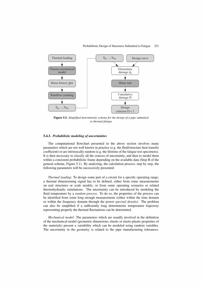
Probabilistic Design of Structures Submitted to Fatigue 251
Figure 5.5. Simplified deterministic scheme for the design of a pipe submittedto thermal fatigue
5.4.3. Probabilistic modeling of uncertainties
The computational flowchart presented in the above section involves manyparameters which are not well known in practice (e.g. the fluid/structure heat transfercoefficient) or are intrinsically random (e.g. the lifetime of the fatigue test specimens).It is then necessary to classify all the sources of uncertainty, and then to model themwithin a consistent probabilistic frame depending on the available data (Step B of thegeneral scheme, Figure 5.1). By analyzing, the calculation process, step by step, thefollowing parameters will be successively presented:
Thermal loading: To design some part of a circuit for a specific operating range,a thermal dimensioning signal has to be defined, either from some measurementson real structures or scale models, or from some operating scenarios or relatedthermohydraulic simulations. The uncertainty can be introduced by modeling thefluid temperature by a random process. To do so, the properties of the process canbe identified from some long enough measurements (either within the time domainor within the frequency domain through the power spectral density). The problemcan also be simplified if a sufficiently long deterministic temperature trajectoryrepresenting properly the thermal fluctuations can be determined.
Mechanical model: The parameters which are usually involved in the definitionof the mechanical model (geometric dimensions, elastic or elasto-plastic properties ofthe materials) present a variability which can be modeled using random variables.The uncertainty in the geometry is related to the pipe manufacturing tolerances.

252 Fatigue of Materials and Structures
The uncertainties of the material properties can be characterized by some tests onthe considered materials or, in the absence of available data found in the literature[JOI 02].
Design curve: The design curve was defined earlier from the specimen medianWöhler curve from the passage factors. In section 5.3, a meticulous statistical analysismethodology yielding the probabilistic Wöhler curves was presented. The passagefactors shall now be studied.
Passage factors γN = 20 and γS = 2, defined above, have been introducedto the deterministic design in order to conservatively cover two effects of a verydifferent nature: the natural variability of the lifetime under fatigue between laboratoryspecimens on the one hand and the structure within its real environment on the otherhand. These factors can then be split as follows:
γN = γNdisp · γN
passage
γS = γSdisp · γS
passage
[5.17]
In these equations, γ.disp and γ.
passage correspond to the part connected to eacheffect. Some empirical decompositions can be found in the literature, for instanceγNdisp = 2 when γN = 20 and γS
disp = 1.19 when γS = 2 [COL 98]. However,there is no real agreement regarding this topic as the data are mostly empirical andmuch connected to the type of material tested. The additional variables γS
passage andγNpassage are called specimen-to-structure passage factors and allow us to consider the
effects of the size of the structure, its surface finish and the environmental conditions(especially regarding temperature and chemistry in nuclear engineering, etc.).
It is obvious that these passage factors that connect the crack initiation time ofa specimen to that of a structure made of the same material (microstructure) cannotbe physically measured. In order to get a rigorous probabilistic representation, it isthen necessary to rely on some probabilistic inverse methods, which allow the factorsand their distributions to be estimated from both data on specimens and structures(e.g. some pipe scale models that are typical of the considered real system, like theINTHERPOL tests described in [CUR 04, CUR 05])). Details about this identificationtechnique are not reported in this chapter, see [PER 07a] for a detailed presentation.
5.4.4. Random cumulative damage
The cumulated damage D can be considered as the result of the computationalchain, as shown in Figure 5.5. If we now consider the input parameters of each sub-model of this chain to be random (thermomechanical model, extraction of the cycles,

Probabilistic Design of Structures Submitted to Fatigue 253
design curve, etc.), the cumulated damage becomes random. The natural definition ofthe random elementary damage related to a single cycle with a fixed amplitude S is:
d(S, ω) ≡ 1/Nstruc(S, ω) = 1/min[NS(ω)/γ
Npassage , NγS
passage(ω)
][5.18]
In this equation, Nstruc(S, ω) is the lifetime of the structure under a loading with aconstant amplitude S, which is connected to the probabilistic Wöhler curve NS(ω)by the passage factors. If the thermomechanical calculation followed by the rainflowcounting leads to a number of cycles Nc (possibly random), the cumulated randomdamage D(ω) is then written:
D(ω) =
Nc∑i=1
d(Si(ω), ω) [5.19]
In this equation, the random property of the damage comes from both:– the randomness of the loading, which is propagated through the mechanical
model for evaluating the amplitude of the cycles Sk(ω), k = 1, . . . , Nc;– the randomness of the material fatigue strength, through the Wöhler curve.
In the case of a stationary random loading, for some loading sequences whichare long enough, the number of extracted cycles Nc becomes high and can then beconsidered in a first approximation as being deterministic [TOV 01]. The amplitudesof the extracted cycles can then be continuously represented by their probabilitydensity function fS(s). This leads to the “continuous” definition of the randomcumulated damage:
D(ω) =
∞∫0
Nc fS(s) dS
Nstruc(S, ω)= Nc ES
[1
Nstruc(S, ω)
][5.20]
where ES [.] stands for the mathematical expectation with respect to the probabilitydensity function of amplitudes fS(s). Assuming Miner’s linear cumulative damageassumption and a significant number of independent extracted cycles, the cumulativedamage defined by equation [5.19] has been proven to converge towards the onedefined by equation [5.20] [SUD 03b].
The previous continuous formulation can be successfully applied to a fatigueassessment in the frequency domain. From the power spectral density (PSD) of theloading, and if the mechanical model is linear, the PSD of the resulting equivalentstress can be obtained. Some empirical formulae, such as those proposed by Dirlik[BEN 06, DIR 85], allow the probabilistic density of the extracted cycles using therainflow method to be constructed, which can then be substitued into equation [5.20].Readers are referred to the work by Guédé [GUÉ05, chapter 6, GUÉ07].

254 Fatigue of Materials and Structures
5.4.5. Application: probabilistic design of a pipe under thermalfatigue conditions
5.4.5.1. Problem statement and deterministic model (step A)
To illustrate the different concepts presented in this section, a piece of pipe, that isof a circuit of a pressurized water reactor, will be considered. The results obtainedby [GUÉ 05], Chapter 7, are reported. The reader can check this reference for acomprehensive parametric analysis of the problem under different loadings, as wellas for a comparison of the probabilistic approaches within both time and frequencydomains.
Let us consider a section of a pipe with a radius Rint and a thickness t, subjectedto a fluid temperature at the inner wall modeled by a random Gaussian process θ(t, ω),whose average temperature is equal to 130°C and standard deviation is equal to 20°C.This process is a pseudo-white noise whose power spectral density is constant withinthe [0 ; 5 Hz] interval. From these data, a realization θ(t) is simulated on a long enoughtime interval ([0 ; 360 s] here) and this signal is then considered as being periodicallyreproduced. The first 10 seconds of the signal are represented in Figure 5.6. Thecomponent service duration is considered to be equal to Nseq = 10, 000 sequences of360 seconds.
Figure 5.6. Probabilistic design of a pipe submitted to thermal fatiguetemperature history
The stress state within the pipe can be calculated using a 1D axi-symmetricalmodel with generalized plane strains (the strain component εzz is assumed to beconstant within the thickness). According to the RCC-M code, an elastic calculation iscarried out. The fluid temperature is transferred to the inner wall of the pipe througha fluid/structure heat transfer coefficient. The external wall of the pipe is insulated

Probabilistic Design of Structures Submitted to Fatigue 255
(preventing the loss of heat). Due to the simplified form of the model, the obtainedstress tensor is diagonal and its components are varying synchronously in time. Theorthoradial stress time history σθθ(t) may be considered to perform the rainflowcounting. The amplitudes of the extracted cycles are corrected by the Goodman linewithin the Haigh diagram in order to consider the average stress.
5.4.5.2. Probabilistic model (step B)
The different random variables modeling the uncertainties on the parameters of themodel are presented in Table 5.1. The choice of the probability distribution functionsand their parameters (step B) was performed as follows3:
– The properties of the materials are modeled by some lognormal laws which areusually well adapted to this type of parameter (being positive). The coefficients ofvariation have to be fixed by experts. The geometry parameters are also modeled bylognormal distributions, with a variation coefficient made high on purpose.
– The variables physically bounded (Poisson ratio, passage factors) are modeledby Bêta distributions.
– The probabilized Wöhler curve (equation [5.9]) was established by the Guédémethod (section 5.3.3.1) and is written as follows:
N(S, ω) = exp [(−2.28 log(S − 185.9) + 24.06 ) (1 + 0.09 ξ (ω))] [5.21]
where N(S, ω) is the crack initiation time of the specimens.
5.4.5.3. Reliability and sensitivity analysis (step C&C’)
The probability of crack initiation is studied for a prescribed number of operatingsequences Nseq. To do so, the following limit state function g is defined (the negativevalues of g correspond to the values of the parameters leading to failure):
g (Nseq,X) = 1−Nseq dseq(X) [5.22]
where dseq(X) stands for the random cumulative damage related to a sequence of360 seconds of operation, and X stands for the vector of the random variables listedin Table 5.1.
By using the FORM method (Appendix A, section 5.7), a probability of crackinitiation is obtained: Pf = 8.59.10−2 for a service life of 10,000 sequences. Thisresult is confirmed by some importance sampling, which finally give Pf = 7.65.10−2.
The form method used for the calculation of the initiation probability also providesthe importance factors of the different random variables, which allows the input
3. The data used for the calculation (especially the distribution parameters) does not representany real structure.

256 Fatigue of Materials and Structures
Parameter Distribution Mean value V.C †
Internal radius Rint lognormal 127.28 mm 5%Thickness t lognormal 9.27 mm 5%Heat capacity ρCp lognormal 4,024,000 J/kg 10%Thermal conductivity λ lognormal 16.345 W.m−1.K−1 10%Heat transfer coefficient H lognormal 20,000 W.K−1.m−2 30%Young module E lognormal 189,080 MPa 10%Poisson rotio ν Bêta [0.2; 0.4] 0.3 10%Thermal dilatation coefficient α lognormal 16.95 10−6 10%Yield stress Sy lognormal 190 MPa 10%Ultimate strength Su lognormal 496 Mpa 10%Passage factor γN
passage Bêta [7; 11] 9.39 10%Passage factor γS
passage Bêta [1; 2] 1.68 10%Scattering of the fatigue data Gaussian 0 Standard value: 1ξ (equation [5.9])† coefficient of variation, equal to the ratio of the standard deviation and the mean value.
Table 5.1. Probabilistic design of a pipe submitted to thermal fatigue:probabilistic model of the parameters
Parameter Importance factor (%)Scattering of fatigue data ξ 40.3Heat transfer coefficient H 20.8Passage factor γS
passage 13.7Young’s module E 8.9Thermal dilatation coefficient α 8.9Other variables 7.4
Table 5.2. Probabilistic design of a pipe submitted to thermal fatigue:importance factors
parameters of the model to be ranked according to their respective contribution tothe fatigue. These normalized factors (given in percentages) are listed by decreasingorder in Table 5.2.
Beyond the strict numerical values of these importance factors (which depend onthe probability density functions chosen for modeling the input parameters), the ordersof magnitude as well as the obtained classification lead to some observations. It clearlyappears that the main parameters that mainly explain the variability of the structurecrack initiation time is the scattering of the endurance of the specimens (modeled inthe probabilistic Wöhler curves). Then there are the fluid/structure transfer coefficient,the passage factor γS
passage increasing the stress amplitudes in the high cycle domain,

Probabilistic Design of Structures Submitted to Fatigue 257
and finally the Young’s modulus and the thermal dilatation coefficient. The otherparameters have a negligible importance, which means that their variability doesnot contribute to the variability of the cumulative damage (and thus to the initiationprobability). As a consequence, they can be considered to be deterministic in this typeof analysis.
5.4.6. Conclusion
In this section, we propose a general frame to address the issue of uncertainties inthe design of loaded the structure submitted to fatigue, stressing on every uncertaintysource observed in the computational chain. As an illustrative example, the probabilityof crack initiation within a pipe submitted to thermal fatigue was estimated. Aquantification of the influence of every uncertain parameter on this probability wasobtained. Even if caution is required for the values, some usefully qualitativeconclusions can still be drawn for the comprehension of the problem.
5.5. Probabilistic propagation models
5.5.1. Introduction
As observed for crack initiation, the propagation of pre-existing cracks undercyclic loading shows some randomness. An extensive experimental study performedby Virkler et al. [VIR 78] on some alumina 2024-T3 specimens clearly shows thescattering of crack propagation among identical specimens (Figure 5.7): 68 pre-cracked (initial size a0 = 9 mm) rectangular sheets with a length of L = 558.8 mm,a width of w =152.4 mm and a thickness of t =2.54 mm) are loaded undertension-compression (∆σ = 48.28 MPa, R = 0.2). The tests are stopped whenthe length of the crack reaches 49.8 mm. It can be observed that this final lengthis reached between 223,000 and 321,000 cycles depending on the specimens with aalmost continuous distribution in between.
By observing Figure 5.7, two types of randomness can be noticed regarding crackpropagation:
– a global scattering of the curves, whose shapes are similar although the numberof cycles varies;
– for each curve, a local irregularity, which shows that the successive incrementsof the crack size along a given trajectory are also random.

258 Fatigue of Materials and Structures
Figure 5.7. Crack propagation – experimental propagation curves accordingto Virkler et al. [VIR 78]
5.5.2. Deterministic model
Crack propagation under cyclic loading is usually modeled using the Paris-Erdogan law [PAR 63] ([BAT 10], Chapter 6):
da
dN= C (∆K)
m [5.23]
In this equation, a is the length of the crack, ∆K is the amplitude of the stressintensity factor for a cycle with an amplitude equal to ∆σ and (C,m) are the typicalparameters of the studied material. In the case of a sheet with a width of w bearing acrack in its core, the amplitude of the stress intensity factor is given by:
∆K = ∆σ F( a
w
)√πa F
( a
w
)=
1√cos
(π a
w
) fora
w< 0.7 [5.24]
where F(aw
)is the Feddersen correction factor.
To reproduce the global scattering of the experimental curves using simulation,the parameters of Paris’ law [5.23] can be made random: this is the approach used

Probabilistic Design of Structures Submitted to Fatigue 259
from now on in this chapter. For each sample of parameters (C, m), a propagationcurve is obtained and this curve can reproduce the general shape of the experimentalcurves. However, the modeling of the irregularities of the curves needs the Paris-Erdogan law to be modified by introducing a random process for modulating the sizeincrements during the propagation itself. This type of approach has been studied byDitlevsen and Olesen [DIT 86], Yang and Manning [YAN 96]. A detailed review canbe obtained from [ZHE 98].
5.5.3. Probabilistic model of the data
For each crack propagation curve, the best-fit couple of parameters (C,m) may beestimated using an optimization procedure, which leads to a sample set. A statisticaltreatment of this sample set can then be carried out to infer the best probability densityfunctions. Kotulski [KOT 98] shows that parameters m and logC may be reasonablyrepresented by truncated normal distributions (Table 5.3).
Parameter Distribution Boundaries Average Variation coefficientm normal truncated [−∞; 3.2] 2.874 5.7%logC normal truncated [−28; +∞] -26.155 3.7%
Correlation coefficient: ρ = −0.997
Table 5.3. Crack propagation – probability distribution functions of(logC , m) of Paris law for the Virkler tests [KOT 98]
(da/dN given in mm/cycle)
A strong correlation between both m and logC parameters can be observed(Figure 5.8), which leads us to think that a single and unique underlying parametermight exist whose variability from one specimen to another explains the dispersion ofthe propagation curves.
5.5.4. Propagation prediction
From the Paris model and the probabilistic description of the propagationparameters given in Table 5.3, a cluster of propagation curves can be obtained usingthe Monte Carlo simulation. This leads to a confidence interval (e.g. at a confidencelevel of 95%) regarding the crack length as a function of the number of applied loadingcycles. Figure 5.9 shows the obtained median propagation curve as well as the 2.5%and 97.5% quantiles.
It appears that the scattering observed from the simulated curves has the sameorder of magnitude as that observed on the experimental curves, which validates the

260 Fatigue of Materials and Structures
Figure 5.8. Crack propagation – sample of the parameters of theParis-Erdogan law for the Virkler tests (da/dN given in mm/cycle)
Figure 5.9. Crack propagation – prediction of the median propagation curveand of the 95% confidence interval
statistical treatment of the (logC , m) data previously carried out (see [BOU 08] fora detailed investigation of the influence of the correlation between logC and m on thepredictions).
Nevertheless, the results presented in Figure 5.9 do not give much information inan industrial context where the best prediction of the length of the crack, as a functionof the number of applied cycles, is required. The graph only leads to the conclusionthat a crack with an initial size of 9 mm will reach a size ranging from 23.5 and35.8 mm after 200,000 cycles with a probability of 95%. It is then obvious that a betterestimation is required to assess, for instance, an inspection planning. The followingsection will focus on how to combine the previous results with the measurements

Probabilistic Design of Structures Submitted to Fatigue 261
performed on a structure of interest during the initial phase of propagation, in order toreduce the confidence interval of the prediction.
5.5.5. Bayesian updating crack propagation models
5.5.5.1. Introduction
Bayesian statistics allows us to combine some prior information on the parametersof a probabilistic model with some measurement data. The reader who is unfamiliarwith these concepts can get more information from Appendix A in section 5.7. Inthe context of probabilistic mechanics, the Bayesian framework can be applied toconsistently combine, on the one hand, the predictions of a model whose uncertaininput parameters are modeled by random variables, and on the other hand, themeasurements of the response of the real mechanical system which was modeled.For the precise example of crack propagation, some measurements of the crack lengthobtained for different numbers of cycles at the early stage of propagation may beintroduced in order to update the prior prediction which revealed inaccurate (as seenfrom the previous section).
5.5.5.2. Ingredients for a Bayesian approach to crack propagation
The probabilistic propagation model developed in section 5.5.4 is made of thecrack propagation model (Paris-Erdogan law) and the probabilistic model of theparameters. The truncated normal distributions (Table 5.3) are considered as priorinformation (regarding the Bayesian vocabulary) on the propagation parameters in thecase of 2024-T3 aluminum.
A particular specimen is now studied and the test trajectory corresponding tothe slowest propagation is for the sake of illustration chosen. Figure 5.10 clearlyshows that this test is singular since the propagation curve is largely outside the 95%confidence interval on the prior prediction.
To compare the observations and the predictions, a measurement/model error isusually defined, which considers the measurement of a physical quantity never to beperfectly accurate and the entire mathematical model of the real world to always bemore or less imperfect. Thus the following link between observations and predictionis used:
yobs = M(x) + e [5.25]
where yobs is the measured value and M(x) is the prediction of the model for the“true value” x of the vector of the input parameters. This true value is usuallyunknown, but it is assumed that it corresponds to a specific realization of vector X .The measurement/model error e is supposed to be a realization of a random variableof prescribed distribution (usually Gaussian, with mean value equal to zero and with

262 Fatigue of Materials and Structures
Figure 5.10. Crack propagation – a priori prediction of the propagation (median curve and95% confidence interval) and slowest experimental propagation curve
standard deviation σe). These assumptions lead us to think that yobs is a realization ofa random variable Yobs whose conditional distribution with repect to X = x reads:
Yobs|X = x ∼ N(M(x);σ2
e
)[5.26]
The previous equation then allows the formulation of a likelihood function forthe observations and calculation of an a posteriori for vector X within the Bayesianframework.
5.5.5.3. Bayesian updating methods
The theoretical aspects of the Bayesian updating of mechanical models fromobservations go beyond this chapter’s main topic. The interested reader can get moreinformation from [PER 08]. To summarize, two main types of resolution methods canbe distinguished regarding this issue:
– The methods which will update the prior probabilistic model of the inputparameters of the model (here, the prior probability density functions of logC and m)from the measurements of the system response, and which then allow an a posterioridistribution to be estimated [PER 07b]. The propagation of this new a posterioriprobabilistic model will allow an updated confidence interval to be calculated on thepropagation curve. From an algorithmic point of view, the Markov chain Monte Carlomethods (MCMC) [ROB 96] are well adapted to the simulation of the a posterioridistributions.
– The methods which directly deal with the updating of the model response bydefining a confidence interval, conditionally to the observations. These methods relyon the FORM approximation method that is used in structural reliability analysis[PER 07c, SUD 06].

Probabilistic Design of Structures Submitted to Fatigue 263
5.5.5.4. Application
The evolution of the crack length during the first part of the propagation issupposed to be measured for a few values of the number of cycles (lower than100,000). The Bayesian approach will allow the prediction to be updated, whichmeans that a 95% confidence interval on the propagation curve will be re-estimatedconsidering the measurement data. In this case, five measured values reported inTable 5.4 are considered.
Crack length (mm) Number of cycles9.4 16,34510.0 36,67310.4 53,88311.0 72,55612.0 101,080
Table 5.4. Crack propagation measurements of the crack length on aparticular sample at an early stage of propagation
The updated median curve and the 95% confidence interval are plotted inFigure 5.11. It clearly appears that the updated prediction agrees with the observations,and that the confidence interval is significantly reduced compared to the priorprediction. The length of the crack at 200,000 cycles, predicted once updating hasbeen performed, ranges from 17.4 to 19.8 mm, with a 95% probability, the measuredvalue corresponding to the highest value.
Figure 5.11. Crack propagation – a priori and posteriori prediction of the crack propagationcurve (median curve and 95% confidence interval). The squares correspond to the
measurements used for the updating; the black and white squares correspond to the rest of theconsidered experimental curve

264 Fatigue of Materials and Structures
It is important to note that the probabilistic formalism previously presented allowsus to represent the model error: indeed, the experimental measurements of the cracklength are very accurate and the measurement error can thus be considered as equalto zero. In contrast, the simplified Paris law model does not clearly allow theirregularities from the propagation curve to be reproduced. However, the modelerror introduced within the method (standard value σe = 0.2 mm for the numericalapplication) allows a satisfying confidence interval to be obtained. Such a result wouldnot be obtained using the least squares fitting method, of a Paris curve on the fivemeasurements gathered from Table 5.4.
5.5.6. Conclusion
In this section, the general scheme of the uncertainty modeling was applied tocrack propagation using the classical Paris-Erdogan model. The observed scatteringon the crack propagation rate for identical specimens was well reproduced bypropagating the uncertainties identified on parameters (logC, m) through the Parislaw. The 95% confidence interval tends to become very wide when the number ofcycles increases. Nevertheless, considering the auscultation data (in this case, cracklengths measured at an early stage of propagation) within a Bayesian frameworkallows the predictions to be significantly improved as it gives an updated mediancurve in accordance with the observations and strongly reduces the 95% confidenceinterval.
The probabilistic approaches present the advantage to be used for any type ofunderlying physical model. Thus, the use of the extended finite element method (X-FEM) applied to crack propagation can be coupled with the methods of uncertaintymodeling as presented in section 5.2, see [NES 06, NES 07].
5.6. Conclusion
The random nature of the fatigue phenomenon within materials and structureshas been well-known for many years. Nevertheless, the consistent and rigorousintegration of all the uncertainty sources regarding the design of realistic structuresis an interesting topic. In this chapter, a general methodology of the uncertaintytreatment was described. This methodology can be applied to mechanics and alsoto any domain where the numerical simulation of physical phenomena is necessary(computational fluid, dynamics, thermal problems, neutronics, electromagnetism,chemical engineering, etc.). This general scheme can be applied to the design ofthe fatigue of mechanical parts; either at the crack initiation phase (S −N ) approach)or at the propagation step of existing cracks (Paris-Erdogan approach).
From a general point of view, a certain French cultural reluctance to use theprobabilistic methods in industry can be observed, especially regarding the behavior of

Probabilistic Design of Structures Submitted to Fatigue 265
structures. Most of the design codes (nuclear, aerospace, civil engineering industries)are mainly deterministic (based on conservative design ensured by safety factors),even if some parts of the codified rules (especially the choice of characteristicvalues for the calculation parameters) do have some probabilistic interpretation. Asfatigue analysis is a field where randomness is observed at various levels (materialstrength, loading, etc.) and cannot be reduced, it seems important that the uncertaintyquantification methods are used as a routine in this field in the future.
5.7. Appendix A: probability theory reminder
The aim of this appendix is to recall the basics of probability theory required tounderstand this chapter. It is not a mathematical course on this topic. For furtherinformation on the statistical methods used in this chapter, readers should refer to thebooks by Saporta [SAP 06] and O’Hagan and Forster [OHA 04].
5.7.1. Random variables
The classical axiomatic approach of the probability theory consists of building anabstract probability space triplet (Ω, F , P), where Ω stands for random experiment,F stands for which means set of sub-ensembles of steady Ω by switching to thecomplementary and the finite union, and P () stands for probability measurement.This last allows each event A ∈ F to be connected to its probability P (A) which is areal number ranging from 0 to 1.
In probabilistic engineering mechanics random variables (and therfore the randomvectors) are used to model the uncertainty of the parameters of the mathematical modelwhich describes the mechanical system. A random (real) variable X(ω) is defined asan application X : Ω 7−→ DX ⊂ R. A realization of a random variable x0 ≡X(ω0) ∈ DX is one of the possible values that the parameter, modeled by X , cantake. The term of discrete or continuous variable is used depending on the supportDX (meaning the set of all the possible realizations of the variable) which can bediscrete or be continuous.
A random variable X(ω) is entirely defined by its cumulative distribution function,written as FX(x) : DX 7−→ [0 , 1]:
FX(x) = P (X(ω) ≤ x) [5.27]
The cumulative distribution function evaluated at point x is then the probabilityrandom variable4 X takes values lower than or equal to x. For a continuous random
4. From now on, the dependency on ω is omited for the sake of simplicity. The random variablesare denoted by capital letters while lowercase letters are used for realizations.

266 Fatigue of Materials and Structures
variable, the probability density function is defined by:
fX(x) =dFX(x)
dx[5.28]
Therefore, quantity fX(x) dx stands for the probability that X takes a valueranging from x to x+ dx. By definition, the integral of fX on its definition domain isequal to 1. This is also the limit of FX(x) when x tends towards the upper boundaryof DX . The classical axiomatic approach of the probability theory consists of buildingan abstract probability space defined by the triplet (Ω,F,P), where Ω stands for theoutcome space of the random experiment, F stands for the σ-algebra of events (whichmeans the set of all subsets of Ω that is stable by union and complementary operations)and P() stands for the probability measure, which allows us to assign a probabilityP(A) to each event A ∈ F. For instance, the uniform distribution of an interval [a , b]has a probability density function fU (x) = 1/(b − a) if x ∈ [a , b], and 0 otherwise.A Gaussian distribution (also called normal distribution) N (µ σ) is defined by thefollowing probability density for any x ∈ R:
fN (x) =1
σφ
(x− µ
σ
)[5.29]
where φ(x) is the standard normal probability density function which can be writtenas:
φ(x) =1√2π
e−x2/2 [5.30]
The normal cumulative distribution function, usually written as Φ, is defined by:
Φ(x) =
∫ x
−∞
1√2π
e−t2/2 dt [5.31]
It has no analytical expression, however it is tabulated in such as Excel, Matlab, Scilab,etc.
In this chapter, the lognormal distributions are used. By definition, a randomvariable follows a lognormal distribution if its logarithm follows a Gaussiandistribution. The following equation is then used:
X ∼ LN (λ, ζ) : X = eλ+ζ ξ with ξ ∼ N (0, 1) [5.32]
The probability density of a variable LN (λ, ζ) is written as:
fLN (x) =1
ζxφ
(lnx− λ
ζ
)[5.33]

Probabilistic Design of Structures Submitted to Fatigue 267
The most likely value of a random variable corresponds to the realization x0 whichmaximizes the probability density fX(x): this is what is called the mode. The usualdistributions present a single maximum (they are called uni-modal) but some multi-modal distribution can also be built.
5.7.2. Expected value, moments, and quantiles
The expected value of a random variable is defined as:
E [X] ≡∫DX
x fX(x) dx [5.34]
This is what is usually called the average of X , which is also written as µX . Aslong as the integral is defined, the expected value of a function g(X) can usually bedefined by:
E [g(X)] ≡∫DX
g(x) fX(x) dx [5.35]
The statistical moments mk (respectively centered moments µk) correspond to theparticular case where g(X) = Xk (respectively g(X) = (X − µX)k, k ∈ N):
mk =
∫DX
xk fX(x) dx [5.36]
µk =
∫DX
(x− µX)k fX(x) dx [5.37]
Variance σ2X ≡ µ2 = E(X−µX)2 is the centered moment of the second order.
The standard value of X , written as σX , is the square root of the variance, and thecoefficient of variation (given as a percentage) is the ratio CVX = σX/µX
.
The quantiles of a random variable are defined from the inverse cumulativedistribution function. The quantile xq with an order of q is defined by:
xq : P (X ≤ xq) = q [5.38]
which can also be written as:
xq = F−1X (q) [5.39]
if the cumulative distribution function FX is stricly increasing.

268 Fatigue of Materials and Structures
5.7.3. Maximum likelihood
Step B of the general scheme of the treatment of the uncertainties consists ofproposing a probabilistic model of the input parameters of the mechanical model;that is to say, to prescribe a probability density function fX(x) for the vector X ofthese parameters.
In this chapter, only the case where the input variables can be considered asindependent is studied : fX(x) is then the product of the marginal probability densityfunctions fXi . If we can rely on experimental data E = x(1), . . . , x(Q) for theparameters, the statistical inference techniques can be used in order to determinea probability distribution that is consistent with the available data. The parametricinference consists of assuming a specific form for the probability density fX (e.g.Gaussian, lognormal, etc.) and then in estimating the parameters of this density sothat it better reproduces the sample. Let f(X;θ) be this density where f() is a knownfunction (e.g. equation [5.29]) and θ is the vector of parameters that shall be estimated(e.g. θ = (µ , σ)). The likelihood function of the sample set is defined as:
L(θ ; E) =Q∏i=1
f(x(i);θ) [5.40]
Once the sample is known, this likelihood function only depends on θ. Themaximum likelihood principle indicates that the best choice of the parameters (calledθ) is then the one which maximizes the previous function, or equivalently minimizesthe log-likelihood:
θ = argminθ
[− log L(θ ; E)] = argminθ
[−
Q∑i=1
log f(x(i);θ)
][5.41]
Usually, from the observation of sample set E using the tools of descriptivestatistics (e.g. histograms [SAP 06, Chapter 5]), different choices are possiblefor f(X;θ). The best parameters are then estimated for each choice and thehypotheses are validated a posteriori using goodness-of-fit tests (e.g. the Kolmogorov-Smirnov test, the Anderson-Darling test, χ2, etc. [SAP 06, Chapter 14]). The mostrelevant distribution can eventually be selected using likelihood criteria such as AIC(Akaike Information Criterion) or BIC (Bayesian Information Criterion) [SAP 06,Chapter 19]).

Probabilistic Design of Structures Submitted to Fatigue 269
5.7.4. Bayesian inference
Bayesian statistics is a branch of statistics coming from Bayes’ theorem which isan elementary result of the probability theory, which states that for two random eventsA and B:
P (A|B) =P (B|A) P (A)
P (B)[5.42]
where P (A|B) is the conditional probability of A knowing B and is equal bydefinition to P (A ∩B) /P (B). The previous result can easily be applied to theprobability density functions (respectively conditional probability density functions)of random variables.
The Bayesian approach consists in integrating some prior information on theparameters θ to be estimated. Not only a family of distribution f(X;θ) is chosenbut also a probability density function pΘ(θ) (called prior distribution) is definedfor the so-called hyper-parameters θ. For instance the Gaussian distribution f(X;θ)with a mean value µ and a standard value σ is selected and in addition, the mean valueµ is assumed to a priori vary between a lower and an upper bound, which comes tomodeling the hyper-parameter µ by a uniform variable between these two bounds. Thea posterior distribution fΘ can then be deduced by combining the prior distributionand the likelihood function:
f ′′Θ(θ) = cL(θ ; E) pΘ(θ) [5.43]
where L is the likelihood function defined in equation [5.40] and c is a normalizationfactor which ensures that f ′′
Θ is a probability distribution function. This equation issimilar in principle to equation [5.42] and can be read as follows: the distribution ofΘ conditionally to the observations E is equal to the prior distribution multiplied bythe likelihood function.
Focusing on the initial problem, which is to propose the best possible probabilisticmodel for parameter X , the mean value or the a posteriori mode of f ′′
Θ can be chosenas the best parameter.
In the case of updating the predictions of a model Y = M(X) by someobservations Yobs = y(1), . . . , y(Q) (see section 5.5.5), the prior probabilisticmodel is defined for X (which acts as hyper-parameters Θ in the above description)and the a posteriori distribution f ′′
X is eventually propagated through the physicalmodel M.

270 Fatigue of Materials and Structures
5.7.5. Reliability analysis and FORM method
A structural reliability problem is set up from the following ingredients:a mechanical model M, a probabilistic model for its input parameters X(i.e. a probability density function fX(x), and a failure criterion5 (see [LEM 08]for a pedagogical introduction to structural reliability). It can be mathematicallyformulated using a limit state function (also called performance function) g(X) whichshall take negative (respectively positive) values for the realizations of X such thatthe mechanical system fails (respectively does not fail). The set of points x such thatg(x)= 0 defines the limit state surface. A common situation corresponds to the casewhen a quantity of interest Y (obtained as the response of a mechanical model) shallnot be greater than a prescribed threshold y. The associated limit state function thenreads:
g(X) = y −M(X) [5.44]
The failure probability is then given by:
Pf ≡ P (g(X) ≤ 0) = P (M(X) ≥ y) =
∫Df
fX(x) dx [5.45]
where Df = x : g(x) ≤ 0 stands for the failure domain. The Monte Carlosimulation method allows us to evaluate the above failure probability quite easily:the input random vector is sampled, which means that an artificial sample set of inputvectors is created according to fX , say X = x(1), . . . ,x(N). For each randomvector x(i) the response M(x(i)) and then the criterion g(x(i)) are evaluated. Thefailure probability is estimated by the number of times Nf the calculation leads to anegative value of g(x(i)), divided by the total number of samples N :
Pf =Nf
N[5.46]
This method is not applicable in practice for problems where the failure probabilityto be evaluated is low (say from 10−2 to 10−6): indeed, about N = 400 × 10k
realizations of X are needed to get a 5% accurate estimation of a failure probabilitywith an order of magnitude 10−k. The Monte Carlo simulation is therefore notpossible, due to its cost, when each evaluation of M corresponds to a calculationrelying on finite elements that may take several minutes or hours.
The FORM method is an approximation method which provides an estimation ofPf at low computational cost. The vector of parameters X is first transformed into a
5. Failure corresponds here to the “non-fulfilling of a performance assigned to the system” andnot necessarily to the collapse of the considered mechanical system.

Probabilistic Design of Structures Submitted to Fatigue 271
vector of standard normal random variables X = T (ξ), which allows equation [5.45]to be recast as:
Pf ≡ P (g(T (ξ)) ≤ 0) =
∫Df=ξ:g(T (ξ))≤0
(2π)−n/2 e−∥ξ∥2/2 dξ [5.47]
where n is the dimension of ξ. In this equation, the integrands exponentially decreasewith |ξ|2. Therefore, the points of the integration domain (failure domain) thatcontribute the most to the integral are those points that are close to the origin of thisstandard normal space. Thus the design point ξ∗ is first computed, which is the pointof the failure domain that is the closest to the origin of the space. The limit statesurface is then linearized around ξ∗. The failure probability is then proven to beequal to:
Pf,FORM = Φ(−β) [5.48]
where β = |ξ∗| is the Hasofer-Lind reliability index.
For a reliability problem in which the dimension of the input vector X is lowerthan 10, the FORM method usually yields good results for a number of evaluations ofg (which are necessary to find the designing point ξ∗) lower than 100. This numberis independent of the order of magnitude of Pf in contrast to Monte Carlo simulation.However FORM only provides an approximation of Pf and it is not possible to provethat this FORM result is close to the true value of Pf or not, and/or that the resultis conservative or not. Some additional techniques like importance sampling shall beused to validate the FORM results [LEM 05].
5.8. Bibliography
[AFC 00] AFCEN, Règles de Conception et de Construction des Matériels des IlotsNucléaires, (RCCM), June 2000, Paris.
[AFN 90] AFNOR, Produits Métalliques – Pratique des Essais de Fatigue Oligocyclique,Norme A03-403, AFNOR, 1990.
[AFN 91] AFNOR, Produits Métalliques – Essais de Fatigue: Traitement Statistique desDonnées, Norme A03-405, AFNOR, 1991.
[ALE 04] F. ALEXANDRE, Aspects probabilistes et microstructuraux de l’amorçage desfissures de fatigue dans l’alliage Inco 718, PhD Thesis, Ecole Nationale Supérieure desMines de Paris, 2004.
[AMZ 94] C. AMZALLAG, J.-P. GEREY, J.-L. ROBERT, J. BAHUAUD, “Standardization ofthe Rainflow counting method for fatigue analysis”, Int. J. Fatigue, vol. 16, pp. 287-293,1994.
[BAS 60] F. BASTENAIRE, Etude statistique et physique de la dispersion des résistances et desendurances à la fatigue, PhD Thesis, Faculté des Sciences de l’Université de Paris, 1960.

272 Fatigue of Materials and Structures
[BAT 10] C. BATHIAS, A. PINEAU, Fatigue of Materials: Fundamentals, ISTE, London andJohn Wiley & Sons, New York, 2010.
[BEN 06] D. BENASCIUTTI, R. TOVO, “Comparison of spectral methods for fatigue analysisof broad-band Gaussian random processes”, Prob. Eng. Mech., vol. 21, pp. 287-299, 2006.
[BOU 08] J.-M. BOURINET, M. LEMAIRE, “FORM sensitivities to correlation: applicationto fatigue crack propagation based on Virkler data”, Proc. 4th Int. ASRANet Colloquium,Athens, 2008.
[COL 98] COLLECTIF, Re-evaluation of Fatigue Analysis Criteria, EE/S 98.317 Report,Framatome, 1998, (Final report to CEC-DG XI contract B4-3070/95/000876/MAR/C2).
[CUR 04] F. CURTIT, “INTHERPOL thermal fatigue tests”, Proc. 3rd Int. Conf. Fatigue ofReactor Components, NEA/CSNI/R, Seville, 2004.
[CUR 05] F. CURTIT, J.-M. STÉPHAN, “Mechanical aspect concerning thermal fatigueinitiation in the mixing zones piping”, Trans. 18th Int. Conf. on Struct. Mech. in ReactorTech. (SMiRT 18), Beijing, China, 2005.
[DIR 85] T. DIRLIK, Application of computers in fatigue analysis, PhD thesis, University ofWarwick, United Kingdom, 1985.
[DIT 86] O. DITLEVSEN, R. OLESEN, “Statistical analysis of the Virkler data on fatigue crackgrowth”, Eng. Fract. Mech., vol. 25, pp. 177-195, 1986.
[DIT 96] O. DITLEVSEN, H. MADSEN, Structural Reliability Methods, J. Wiley and Sons,Chichester, 1996.
[DRO 04] J. DROESBEKE, J. FINE, G. SAPORTA, Méthodes Bayésiennes en Statistique,Editions Technip, 2004.
[EDF 06] EDF, R&D DIVISION, Code_Aster: Analyse des Structures et Thermo-mécaniquepour des Études et des Recherches, V.7, 2006, http://www.code-aster.org.
[GHA 91] R. GHANEM, P. SPANOS, Stochastic Finite Elements – A Spectral Approach,Springer Verlag, 1991.
[GUÉ 05] Z. GUÉDÉ, Approche probabiliste de la durée de vie des structures soumises à lafatigue thermique, doctorate thesis, Université Blaise Pascal, Clermont-Ferrand, 2005.
[GUÉ 07] Z. GUÉDÉ, B. SUDRET, M. LEMAIRE, “Life-time reliability based assessment ofstructures submitted to thermal fatigue”, Int. J. Fatigue, vol. 29, no. 7, pp. 1359-1373, 2007.
[JOI 02] JOINT COMMITTEE ON STRUCTURAL SAFETY, JCSS Probabilistic Model Code,JCSS 2002, http://www.jcss.ethz.ch.
[KOT 98] Z. A. KOTULSKI, “On efficiency of identification of a stochastic crack propagationmodel based on Virkler experimental data”, Arch. Mech., vol. 50, no. 5, pp. 829-847, 1998.
[KRE 83] P. KREE, C. SOIZE, Mécanique Aléatoire, Dunod, 1983.
[LAC 97] B. LACAZE, C. MAILHES, M. MAUBOURGUET, J.-Y. TOURNERET, Probabilitéset Statistique Appliquées, Cépaduès Editions, 1997.
[LEM 05] M. LEMAIRE, Fiabilité des Structures – Couplage Mécano-fiabiliste Statique,Hermès, 2005.

Probabilistic Design of Structures Submitted to Fatigue 273
[LEM 08] M. LEMAIRE, “Approche probabiliste du dimensionnement – Modélisation del’incertain et méthode de Monte-Carlo”, Techniques de l’Ingénieur, BM 5003-5004, 2008.
[LEM 09] M. LEMAIRE, Structural reliability, John Wiley & Sons, 2009.
[LOR 05] S. LORÉN, M. LUNDSTRÖM, “Modelling curved S–N curves”, Fatigue Fract.Engng. Mat. Struct., vol. 28, pp. 437-443, 2005.
[MEL 99] R.-E. MELCHERS, Structural Reliability Analysis and Prediction, John Wiley &Sons, 1999.
[MIN 45] M. MINER, “Cumulative damage in fatigue”, J. Appl. Mech., vol. 9, pp. 159-164,1945.
[NES 06] L. NESPUREK, J.-M. BOURINET, A. GRAVOUIL, M. L., “Some approachesto improve the computational efficiency of the reliability analysis of complex crackpropagation problems”, Proc. 3rd Int. ASRANet Colloquium, Glasgow, 2006.
[NES 07] L. NESPUREK, J.-M. BOURINET, A. GRAVOUIL, M. L., “Probabilistic approachto crack propagation based on XFEM and FORM”, Proc. Fatigue Design 2007, Senlis,France, 2007.
[OHA 04] A. O’HAGAN, J. FORSTER, Kendall’s advanced theory of statistics, Arnold, 2004.
[PAR 63] P. PARIS, F. ERDOGAN, “A critical analysis of crack propagation laws”, Trans.ASME, J. Basic Eng., pp. 528-534, 1963.
[PAS 97] F. PASCUAL, W. MEEKER, “Analysis of fatigue data with runouts based on a modelwith non constant standard deviation and a fatigue limit parameter”, J. Testing Eval., vol. 25,pp. 292-301, 1997.
[PAS 99] F. PASCUAL, W. MEEKER, “Estimating fatigue curves with the random fatigue-limitmodel”, Technometrics, vol. 41, no. 4, pp. 277-290, 1999.
[PER 05] F. PERRIN, B. SUDRET, M. PENDOLA, M. LEMAIRE, “Comparison of twostatistical treatments of fatigue test data”, Proc. Fatigue Design 2005, Senlis, France, 2005.
[PER 06] F. PERRIN, M. PENDOLA, T. MORO, G. MORIN, J.-M. CARDONA, “Completeprobabilistic framework in fatigue design: application to exhaust manifolds”, in: B.TOPPING, G. MONTERO, R. MONTENEGRO (Eds.), Proc. 8th Int. Conf. Comput. Struct.Tech., Las Palmas de Gran Canaria, 2006.
[PER 07a] F. PERRIN, B. SUDRET, F. CURTIT, J.-M. STÉPHAN, M. PENDOLA, “EfficientBayesian updating of structural fatigue design curve using experimental thermal fatiguedata”, Proc. Fatigue Design 2007, Senlis, France, 2007.
[PER 07b] F. PERRIN, B. SUDRET, M. PENDOLA, “Bayesian updating of mechanicalmodels – Application in fracture mechanics”, Proc. 18e Congrès Français de Mécanique(CFM’2007), Grenoble, 2007.
[PER 07c] F. PERRIN, B. SUDRET, M. PENDOLA, E. DE ROCQUIGNY, “Comparison ofMarkov chain Monte-Carlo simulation and a FORM-based approach for Bayesian updatingof mechanical models”, Proc. 10th Int. Conf. on Applications of Stat. and Prob. in CivilEngineering (ICASP10), Tokyo, Japan, 2007.

274 Fatigue of Materials and Structures
[PER 08] F. PERRIN, Intégration des données expérimentales dans les modèles probabilistesde prédiction de la durée de vie des structures, PhD Thesis, Université Blaise Pascal,Clermont-Ferrand, 2008.
[ROB 92] C. ROBERT, L’analyse statistique bayésienne, Economica, 1992.
[ROB 96] C. ROBERT, Méthodes de Monte Carlo par chaînes de Markov, Economica, 1996.
[RUB 81] R.-Y. RUBINSTEIN, Simulation and the Monte Carlo Methods, John Wiley & Sons,1981.
[SAL 00] A. SALTELLI, K. CHAN, E. SCOTT, Eds., Sensitivity Analysis, J. Wiley & Sons,2000.
[SAL 04] A. SALTELLI, S. TARENTOLA, F. CAMPOLONGO, M. RATTO, Sensitivity Analysisin Practice – A Guide to Assessing Scientific Models, J. Wiley & Sons, 2004.
[SAP 06] G. SAPORTA, Probabilités, Analyse des Données et Statistique, TechnipPublications, 2nd edition, 2006.
[SCH 06] C. SCHWOB, L. CHAMBON, F. RONDE-OUSTAU, J. BERNADOU, “Probabilisticassessment of fatigue life using a stress-based fatigue criterion”, in: B. TOPPING, G.MONTERO, R. MONTENEGRO (Eds.), Proc. 8th Int. Conf. Comput. Struct. Tech., LasPalmas de Gran Canaria, 2006.
[SCH 07] C. SCHWOB, Approche non locale probabiliste pour l’analyse en fatigue des zonesà gradient de contrainte, doctorate thesis, Ecole des Mines d’Albi Carmaux, 2007.
[SUD 03a] B. SUDRET, Z. GUÉDÉ, P. HORNET, J.-M. STÉPHAN, M. LEMAIRE,“Probabilistic assessment of fatigue life including statistical uncertainties in the S–N curve”,Trans. 17th Int. Conf. on Struct. Mech. in Reactor Tech. (SMiRT 17) Paper M-232, Prague,Czech Republic, 2003.
[SUD 03b] B. SUDRET, Z. GUÉDÉ, M. LEMAIRE, “Probabilistic framework for fatigueanalysis”, M. MAES, L. HUYSE, Eds., Proc. 11th IFIP WG7.5 Conference on Reliabilityand Optimization of Structural Systems, Banff, Canada, Balkema, Rotterdam, pp. 251-257,2003.
[SUD 05] B. SUDRET, Z. GUÉDÉ, “Probabilistic assessment of thermal fatigue in nuclearcomponents”, Nuc. Eng. Des., vol. 235, pp. 1819-1835, 2005.
[SUD 06] B. SUDRET, F. PERRIN, M. BERVEILLER, M. PENDOLA, “Bayesian updating ofthe long-term creep deformations in concrete containment vessels”, Proc. 3rd Int. ASRANetColloquium, Glasgow, United Kingdom, 2006.
[SUD 07] B. SUDRET, Uncertainty propagation and sensitivity analysis in mechanical models– Contributions to structural reliability and stochastic spectral methods, Habilitation àdiriger des recherches, Université Blaise Pascal, Clermont-Ferrand, France, 2007.
[THO 99] J.-J. THOMAS, G. PERROUD, A. BIGNONNET, D. MONNET, “Fatigue design andreliability in the automotive industry”, European Structural Integrity Society, vol. 23,pp. 1-11, 1999.
[TOV 01] R. TOVO, “On the fatigue reliability evaluation of structural components underservice loading”, Int. J. Fatigue, vol. 23, pp. 587-598, 2001.

Probabilistic Design of Structures Submitted to Fatigue 275
[VIR 78] D. VIRKLER, B. M. HILLBERRY, P. GOEL, “The statistical nature of fatigue crackpropagation”, Trans. ASME, J. Eng. Mat. Tech., vol. 101, no. 2, pp. 148-153, 1978.
[YAN 96] J. YANG, S. MANNING, “A simple second order approximation for stochastic crackgrowth analysis”, Eng. Fract. Mech., vol. 53, no. 5, pp. 677-686, 1996.
[ZHE 98] R. ZHENG, B. ELLINGWOOD, Stochastic Fatigue Crack Growth in Steel StructruesSubjected to Random Loading, Contract report ITL-98-1 for the US Army Corps ofEngineers, The Johns Hopkins University, 1998.
