a program to calculate design and off-design performance...
TRANSCRIPT

A Program to Calculate Des Off-Design Performance of Ga
9
GasTurb User’s Manualign and s Turbines

2 2
Acknowledgments The author wishes to thank MTU Aero Engines for permission to publish the program GasTurb. Many individuals helped in the review of the program and the manual, but in particular I wish to thank my colleagues Hassan Abdullahi, Andreas Danier, Dr. Peter Jeschke and Reinhold Schaber for their valuable comments.
Finally and most importantly I wish to thank my wife and family for their patience and encouragement during long weekends and evenings that went into the writing of the program. The author has used his best effort in preparing this manual and the program GasTurb. However, the author makes no warranty of any kind, expressed or implied, with regards to these programs or the documentation. The author shall not be liable in any event for incidental or consequential damages in connection with, or arising out of the use of these programs.
All rights reserved. Names of products mentioned herein are used for identification purposes only and may be trademarks and/or registered trademarks of their respective companies. Windows is a
trademark of Microsoft Corporation. GasTurb has been compiled with Borland DELPHI
Copyright 2001
J. Kurzke
Printed in Germany Dr.-Ing. Joachim Kurzke - Fax +49 -8131-54886 - email [email protected]
www.gasturb.de

3
Table of Contents 1. Introduction.............................................................. 13
1.1. Installing the program ................................................................13 1.1.1. Program requirements ........................................................13 1.1.2. Installation..........................................................................13 1.1.3. Using a working directory..................................................14 1.1.4. About GasTurb files ...........................................................14
1.2. A single cycle .............................................................................15
1.2.1. Creating a new data set.......................................................16 1.2.2. Switching between SI and Imperial units...........................16 1.2.3. Define composed values.....................................................17 1.2.4. Define iterations .................................................................17 1.2.5. Starting the calculation.......................................................18 1.2.6. Some general hints .............................................................18
1.3. More cycle design calculations ..................................................19
1.3.1. Parametric study.................................................................19 1.3.2. Optimization.......................................................................20 1.3.3. Small effects .......................................................................21 1.3.4. Monte Carlo study..............................................................21
1.4. Off-design calculations ..............................................................23
1.4.1. Correlating the design point with the component maps.....23 1.4.2. Component map format......................................................23 1.4.3. Map scaling example..........................................................26 1.4.4. Input data for off-design simulations .................................28 1.4.5. Variable compressor geometry...........................................28 1.4.6. Limiters ..............................................................................29 1.4.7. Reheat (Afterburning) ........................................................29 1.4.8. Operating line.....................................................................30 1.4.9. Off-design parametric study...............................................30 1.4.10. Calculation of a flight envelope .........................................30 1.4.11. Off-design effects ...............................................................31 1.4.12. Off-design Monte Carlo simulation ...................................31 1.4.13. Mission calculations...........................................................31 1.4.14. Off-design constraints in a cycle design optimisation .......32 1.4.15. Test analysis by synthesis ..................................................32
2. Theory ..................................................................... 33
2.1. Description of some typical engine configurations....................33 2.1.1. Single spool turbojet...........................................................33 2.1.2. Single spool turboshaft.......................................................39

4
2.1.3. Two-spool turboshaft, turboprop ....................................... 45 2.1.4. Inter-cooled recuperated turboshaft ................................... 52 2.1.5. Two-spool unmixed flow turbofan .................................... 61 2.1.6. Two-spool mixed flow turbofan ........................................ 69 2.1.7. Geared turbofan ................................................................. 79 2.1.8. Three-spool mixed flow turbofan ...................................... 89 2.1.9. Intercooled recuperated turbofan ....................................... 99 2.1.10. Variable cycle engine ...................................................... 109 2.1.11. Ramjet.............................................................................. 117
2.2. Details of the calculation ......................................................... 119
2.2.1. Gas properties .................................................................. 119 2.2.2. Intake ............................................................................... 121 2.2.3. Compressor design........................................................... 123 2.2.4. Compression .................................................................... 123 2.2.5. Pressure losses ................................................................. 124 2.2.6. Combustion chamber ....................................................... 125 2.2.7. Turbine design ................................................................. 128 2.2.8. Expansion ........................................................................ 130 2.2.9. Reheat .............................................................................. 131 2.2.10. Nozzle .............................................................................. 131 2.2.11. Propeller........................................................................... 133
2.3. Iteration technique ................................................................... 139
2.3.1. Mathematical background ............................................... 139 2.3.2. Single spool turbojet ........................................................ 141 2.3.3. Two-spool turboshaft, turboprop ..................................... 142 2.3.4. Boosted turboshaft, turboprop ......................................... 144 2.3.5. Unmixed flow turbofan.................................................... 144 2.3.6. Mixed flow turbofan ........................................................ 146 2.3.7. Geared Turbofan.............................................................. 146 2.3.8. Variable cycle engine ...................................................... 146 2.3.9. Other engines ................................................................... 147
2.4. Inlet flow distortion ................................................................. 149
2.5. Transient simulations............................................................... 153
2.5.1. Additions to the steady state model ................................. 153 2.5.2. The control system........................................................... 154 2.5.3. Mathematical procedure .................................................. 155 2.5.4. Transient test analysis...................................................... 156
3. Application examples ............................................. 157
3.1. Cycle design calculations for a single spool turbojet .............. 157 3.1.1. Calculate Single Cycle..................................................... 157 3.1.2. Parametric Study.............................................................. 159 3.1.3. Small Effects.................................................................... 161

5
3.2. Cycle optimization for a helicopter engine ..............................163 3.2.1. Introduction ......................................................................163 3.2.2. Simple cycle parameter study ..........................................163 3.2.3. Realistic optimization.......................................................165 3.2.4. Summary and concluding remarks...................................169
3.3. Off-design calculations for a two-spool turboshaft..................171
3.3.1. Compressor map scaling ..................................................172 3.3.2. Turbine map scaling .........................................................173 3.3.3. Off-design calculation options .........................................173 3.3.4. Limiters ............................................................................174 3.3.5. Operating line...................................................................175 3.3.6. Flight envelope calculation ..............................................176
3.4. Turbofan engines......................................................................177
3.4.1. Engine design for subsonic aircraft ..................................177 3.4.2. Mixed versus unmixed turbofans .....................................180 3.4.3. Engine design for supersonic aircraft...............................181 3.4.4. Engine families.................................................................184
3.5. Test analysis and engine monitoring........................................187
3.5.1. Turbofan test analysis.......................................................187 3.5.2. Test analysis accuracy......................................................188 3.5.3. Comparing a performance simulation with test data........190 3.5.4. Test analyis by synthesis ..................................................190
3.6. Optimization.............................................................................199
3.6.1. The use of optimization....................................................199 3.6.2. A simple example.............................................................202 3.6.3. Cycle selection for a derivative turbofan .........................203
4. Nomenclature ........................................................ 209
4.1. Station Definition .....................................................................209 4.2. Symbols ....................................................................................211 4.3. Units .........................................................................................213 4.4. Limiter codes............................................................................215
5. References ............................................................ 217 6. Frequently asked questions ................................... 219

6

7
What’s new in GasTurb 9 ?
The program GasTurb has been steadily improved the last two years. Many extensions to GasTurb 8 are just small improvements of the program handling. The following changes are major steps forward:
Graphical User Interface:
The standard size of the program windows is now 600*800 pixels which allows to show more information at a glance. There is now room for 20 instead of 10 composed values, for example.
Engine configurations can now be selected from a configuration tree. There are two main branches in this tree: aircraft engines and gas turbines for power generation. The selected configuration is shown schematically as a colored picture.
The nomenclature pictures have been improved in quality. They now also show the actual values that are used for the internal air system simulation. These pictures can be copied to the clipboard and pasted into any word processor or presentation program.
The data arrangements for input and the output are improved. Input data for the internal air system is now on a separate page, and the same is true for the component efficiency and flow modifiers in off-design simulations. The composed values are color marked when inactive or invalid.
On the cycle overview page you can get now explanations for the abbreviated names: click on a name and an explanation including the units will appear. Moreover, an unit converter can be selected from the menu.
T-s and h-s diagrams can be copied to the clipboard, and the results for “small effects” may be shown graphically also.
Plot your results from parametric studies with up to 4 y-axes over the same x-axis. When your study includes turbine design calculations, then maneuver through your results with the arrow keys on the keyboard and see, how the shape of the turbine velocity triangles changes and how the design point moves in the Smith diagram. This makes it easy to find suitable turbine designs with the help of a parametric study.
Scaling the component maps is more simple now; the user interface for this task has been rewritten completely. Scaling special maps for normal off-design simulations and using a given compressor map in common core engine studies is simpler now.
Engine configuration tree
Output advice
Parametric studies and turbine design

8
New Gas Turbine Configurations:
In previous versions of GasTurb the single spool engine configuration could be used for the simulation of a turbojet, a turboshaft and for a turboprop. Now, shaft power generation is dealt with separately, and in this new configuration a recuperator (heat exchanger) may also be selected.
A two-spool straight turbojet configuration has been added. Other new aircraft engines are an inter-cooled recuperated turbofan as a three-spool engine and a variable cycle engine.
You can now select the booster to be mounted on the low or on the high-pressure spool with two turboshaft configurations. Moreover, there is now also a three-spool turboshaft, i.e. a two-spool gas generator combined with a free power turbine.
New calculation methods:
In the opening window you can now choose between the “Novice” and the “Expert” Mode. Use the Novice Mode if you are a beginner in gas turbine performance calculations or if you are interested only in the fundamentals of gas turbine theory. The Novice Mode hides many input data – like, for example, the internal air system descriptors – from the user and makes the program really easy to use.
The Expert Mode opens the door to detailed gas turbine performance simulations and allows all program options to be used.
A fundamental change to GasTurb is the revised representation of the gas properties. The effect of humidity on engine performance may be studied for all engine configurations now. With the gas turbines used for power generation you can also simulate water and steam injection into the burner. The NOx severity index, which is calculated for all engines, allows estimating emissions.
The Generic Fuel replaces the Standard Fuel used in previous versions of GasTurb. The new fuel and its combustion product properties are calculated with the program from Gordon McBride, i.e. the NASA Equilibrium Code. The Generic Fuel data is consistent with the gas properties of the other fuels offered by the program. This was not the case with the old Standard Fuel.
Using new representations for the gas properties leads to small differences in the simulation results compared to previous versions of GasTurb.
Other reasons for small differences in the calculated results are the following:
• Intake calculation was done up to now with γ=1.4. That was changed to the rigorous calculation using true gas properties, including the humidity effect.
• The correlation between the polytropic and the isentropic efficiency is now calculated using the entropy function. Previously, the conversion was done with the mean isentropic exponent.
• A high-pressure turbine map is now used in all off-design calculations. Therefore, both the turbine efficiency and the corrected flow will no longer remain constant as in previous versions of GasTurb.
Single spool turboshaft
Variable cycle engine
More turboshafts
Novice and Expert Mode
New gas properties
Generic fuel
Reasons for small differences compared to GasTurb 8

9
Other improvements to GasTurb are new input options like, for example, influence factors for the compressor flow capacity or the input of P1, T1 and Pamb alternatively to altitude, Mach number and deviation from ISA temperature.
A completely new option in GasTurb is the model-based test analysis and engine condition monitoring. You can compare measured data with your simulation model and automatically find factors that describe the differences between the test result and the simulation. Several different flow analysis methods are offered and a sensor-checking algorithm may also be used.
In previous versions of GasTurb, you could store the ingredients of complex simulation models, like the scaling of special component maps and control schedules in different files. These files had to be reloaded one after the other when the program was restarted. Now you can store this information, together with the definition of composed values and iterations, all in one file, an “Engine Model” file.
The number of iterations during cycle design point studies has been increased from 5 to 10. Moreover, you can define additions to the off-design iteration scheme. This allows iterating delta A8 during the calculation of an operating line such that the surge margin of the compressor of a turbojet, for example, is constant.
Model fidelity has been improved in some areas:
• Burner and reheat (afterburner) efficiencies will vary with a burner loading parameter.
• Nozzle discharge coefficients depend on nozzle geometry (nozzle petal angle) and pressure ratio.
Further improvements are:
• Absolute spool speeds in RPM have been introduced. Enter your data on the "Compressor (LPC, Booster, IPC, HPC) Design" page.
• Extrapolation of turbine maps is permitted up to 200% corrected speed (was previously 120%). This allows very rapid fuel flow reduction during transient simulations.
• The fuel heating value FHV is offered also for off-design as an input quantity.
This description of improvements in GasTurb 9 is not exhaustive, and you will certainly detect some more nice features when using the program. Feel free to contact the author when you have new ideas about making GasTurb easier to use and an even more accurate tool than it is now.
New input options
Engine condition monitoring
Engine Model
User defined off-design iteration
Model fidelity

10

11
How this manual is organized This manual consists of three main chapters. The introduction begins with instructions on how to install the program. Section 1.2 explains the first menus, data input, switching between SI and Imperial units and also contains some general hints. Section 1.3 introduces more sophisticated design calculations like iterations, parametric studies and optimization. Section 1.4 covers off-design calculations.
The second chapter describes the theory of gas turbine performance as implemented in GasTurb. It begins with a description of the thermodynamic cycle calculation for selected engine types, followed by the details of the calculation for the components. Section 2.3 introduces the iteration technique applied in off-design calculations. Next are sections about inlet distortion simulation with the parallel compressor model, about engine test analysis and performance monitoring and finally section 2.6 deals with simulation of transient performance of gas turbines.
In chapter 3 you will find application examples including input and output data that show the capabilities of the program. Section 3.1 explains the various options for design calculations for a turbojet.
The cycle optimization for a helicopter engine is described in section 3.2. It is shown that a simple variation of compressor pressure ratio and burner exit temperature does not yield a realistic result. Only after including many details in the simulation you do get results that are in line with the cycles of real engines.
The off-design calculation for a two-spool turboshaft is a further example. Among other things, section 3.3 will show you how to calculate the shaft power delivered for any point within the flight envelope. How to select an engine design point for typical applications of turbofans for subsonic and supersonic aircraft is discussed in section 3.4.
Chapter 3.5 is devoted to test analysis and engine performance monitoring. Analysis accuracy, comparison of measured data with simulations and Analysis by Synthesis (i.e. model based test analysis) are discussed.
A short introduction into mathematical optimization and two application examples can be found in chapter 3.6.

12

13
1. Introduction
1.1. Installing the program
The copyright of the program and this manual is by the author and as such should not be reproduced or distributed in any form without prior permission from the author.
1.1.1. Program requirements
For running the program GasTurb 9 you need an IBM-PC/AT or an IBM compatible computer (486 processor or better) with VGA color monitor set to 600*800 pixel resolution and a mouse.
To run GasTurb 9 you need Windows 95, 98, Windows NT or Windows 2000 installed on your computer.
1.1.2. Installation
The program is delivered on CD ROM. The welcome screen of the setup program offers five choices:
Deploy it! Click this button to quickly install the application without answering any technical questions. You will be shown the license agreement and after accepting it, the application will be installed straight away.
More Information
Provides access to a ‘readme’ file
Select Components
This allows you to customize the setup by selecting which components will be installed and which not. After making your selection, you will be shown the license agreement and then the software will be installed.
Advanced Options
If you want total control over the setup, click this button. You can change the installation folders and select which components should be installed. Though the actual selection possibilities remain the same, the component selection will show more detail. If you want, it can even show every file that will be copied to your hard disk.
Do Not Install In case the setup was launched by accident.
As you see, the setup program makes life easy for those who don't understand much about computers (click Deploy it, accept the license and it's done) while still allowing power users to keep full control of everything (Advanced Options).
Install GasTurb for Windows in its own, new directory and do not install it in the directory of your previous program version. Some of the files delivered with GasTurb 9 have the same file name as those of previous versions, but different file contents. Mixing the files from different versions of GasTurb will cause a program crash.
Copyright
Updating from a previous GasTurb version

14
1.1.3. Using a working directory
If you want to store your data files and component map files in a directory different from the program, you need to start GasTurb with two command line parameters. Add after the program call (separated by a space) first the path of your data and second the path to your component maps. The working directory, which you specify from the Windows Program Manager as a program item property, must be the directory in which the program resides.
When you have stored the program in directory C:\GasTurb, for example, and want your data stored in directory C:\GasTurb\Data and your component maps in C:\GasTurb\Maps then you must start the program by the following command sequence:
C:\GasTurb\GasTurb9.exe C:\GasTurb\Data C:\GasTurb\Maps
When your file names or directory names contain blanks, then you must include the path names in double quotes:
"C:\GasTurb\GasTurb9.exe" "C:\My Data\GasTurb\Data" "C:\My Data\GasTurb\Maps"
In a network you can store the program in a directory which everybody can access. The different users should store their private data in their own directories for data and component maps.
Note that the standard component maps delivered with the program must reside in the same directory as the program. You can store a copy of these files in your private component map directory.
1.1.4. About GasTurb files
You can use any editor to look at the data. They are pure ASCII files. Do not modify any data set other than through GasTurb commands. This is because the data are read with a specific format and if anything is out of order or placed in the wrong column the result is unpredictable.
There are some more ASCII files delivered with the program, one for each engine type. Their file name extensions are NMS. They contain important information for the program. Do not modify these files because they are essential for the correct interpretation of the data. Note that the *.NMS files are not compatible between the different program versions.
There are many graphic files that contain engine configuration schemes and other pictures. They are stored as Windows metafiles with the extension WMF. Many other programs can read this file format. You may use these files for illustrations in reports, for example. When you do that, you must refer to the source of the graphics and include the GasTurb program as a reference.
Installation on a network
Data files
Pictures

15
1.2. A single cycle
In the program opening window you must at first select an engine configuration either from the engine configuration tree or from the combobox.
When using the combobox then one or several images will show the activated option. Double click an image to enlarge it. The detailed configuration, for example the type of thrust nozzle (convergent or convergent-divergent), will be defined later in the design point definition screen.
Alternatively, you can use the engine configuration tree to select the basic engine type. Click on the little boxes with a + sign to expand the tree or on a box with a – sign to collapse it. The selected engine configuration is shown as a figure to the right of the selection tree. When the selection is not yet concise enough, then you see the figure of an aircraft or a windmill.
Decide wether to use the program in Novice or Expert mode and then select a task from the list of engine design tasks. When you use the program for the first time then you should use the option Calculate Single Cycle.

16
Pressing the button Ok leads you to the data file reading window which shows the example data files that are delivered with the program. The names of all example files start with DEMO. The file extension is composed of three letters and always begins with the letter C that stands for cycle data. The other two letters are associated with the engine type. Cycle data for single spool turbojets, for example, have the file extension CYJ.
This file nomenclature has the advantage that in data selection boxes only those files that are compatible with the type of engine you are currently simulating are offered for loading.
When you read a data file, which has been created with a previous version of GasTurb, then you will get some warning messages. These messages regard input properties that did not exist in the previous program version or that have been renamed. In many cases the missing data are set to reasonable default values, in some cases the dummy value 111111 is introduced.
Old files for the turbojet engine configuration produce many warning messages. The reason for that is that in GasTurb 9 the single spool turboshaft engine is now a separate engine configuration.
You will be prompted to enter a suitable number for the missing data that are indicated by the dummy number 111111. Commencing the calculation with one or more properties having the dummy value will result in an error message.
Storing an old data file on disk from a new version of GasTurb will make the data set compatible with the new version.
GasTurb 9 will not exactly reproduce the numbers from previous program versions because the gas properties are now modelled slightly different.
1.2.1. Creating a new data set
You create a new input data set by modifying an existing data set. There is no option available to create it from scratch.
The data are presented in tabbed notebooks. The input data shown on the pages of the notebook are the only ones that you need for the selected switch position. You will not see any input quantities that are not needed for the type of calculation you have chosen. Data you have entered for a switch position not selected at the moment will not be deleted; it will just not be shown. When you write a set of data to disk, all quantities will be stored, regardless of the switch positions.
You can get help for the nomenclature from the menu on top of the screen and from the help file (look for the topic Nomenclature in the help index). Hold your mouse pointer on one of the buttons below the menu line and you will get a hint about which action will be initiated by pressing the button. Note that often some of the buttons in a row may be dimmed and therefore inactive.
1.2.2. Switching between SI and Imperial units
Click on the button with the red arrow pointing to the right to convert your input data from SI units to Imperial units. The button with the arrow pointing to the left will convert the data from Imperial to SI units.
If you have started with a data set in SI units and you wish to store it on disk in Imperial units, then the data set will automatically be converted before being
Use of old data files with GasTurb 9
Help

17
written to disk. All of the results of the calculations will then be presented in Imperial units. Note that only the design point input window offers the possibility to switch between units.
1.2.3. Define composed values
You may be interested in a quantity which is not directly available as output, such as the temperature ratio across the compressor, T3/T2. You can get the desired value by defining a composed value using values for T2 and T3 that are both in the standard output data set.
Twenty composed values can be defined. The mathematical operations available include +, -, * , / and ^ for exponential expressions. You can also use brackets in your definitions. An example for a complex composed value is
1004,5*T2*((P3/P2)^0,2857-1)
In general, for composed values you can use any previously defined composed value:
cp_val1^0.5+1
You can give composed values a name by using a short text followed by the = sign:
spec. work =1004,5*T2*((P3/P2)^0,2857-1)
This name of the composed value will be used in the list and the graphics output. Note, however, that you must use the short name cp_valxx when you want to use the result of this expression within the definition of another composed value.
The result of an invalid operation like the square root of a negative number will be set to zero. Check the result of any complex formula and use brackets to achieve the intended result.
In the definition of a composed value you can use any input and output properties and also plain numbers. The availability of property names depends on the position of the switches. If turbine design is switched off, for example, then you cannot use geometrical data of the turbine in composed values, since they will not be calculated. You can check the validity of your formulae by clicking on the Check button.
1.2.4. Define iterations
Select this option from the menu or by clicking on the corresponding button, if you want an output quantity to have a specific value. In the turbojet cycle you can, for example, iterate the compressor pressure ratio in such a way that the turbine pressure ratio will be exactly four (this could be a reasonable limit for a one-stage turbine). You have to tell the program both lower and upper limits for the input variable (the compressor pressure ratio). Select those limits reasonably! A cycle with a compressor pressure ratio below one could cause problems.
Whether the iteration converges or not depends very much on the problem being investigated. If there is a solution, the program will find it. Thus, check your data if you do not get convergence.

18
Note, that you can select up to ten variables, thus specifying values for ten output quantities. In addition to keeping the turbine pressure ratio constant, you can keep the thrust constant by iterating engine mass flow, for example. You could also iterate burner exit temperature as a third variable such that the turbine exit temperature is equal to a specified value.
For each of the variables a reasonable range must be specified. If the range is too narrow, then by accident the solution could be excluded and the iteration would fail to converge. A very wide range causes also problems, since the cycle cannot be evaluated with extreme combinations of pressure ratio and turbine inlet temperature. Moreover, a large range for the iteration variables leads to an inaccurate result.
1.2.5. Starting the calculation
After you have selected Ok from the design point input window your present data set will be checked. Then, the thermodynamic calculation will commence. The runtime needed for one example depends both on the engine type (a mixed turbofan takes the longest, a ramjet the shortest) and on your computer. A machine with a 486 CPU without coprocessor will require some patience, while a computer with a Pentium will give you the answer immediately.
Newcomers to the program should play around with the input data of the turbojet and calculate several cycles, thereby getting accustomed to the nomenclature and the units used (press F1 for help).
1.2.6. Some general hints
The data will be saved automatically before the calculation starts. Depending on the engine type, GasTurb uses a specific filename. Any turbojet example is called LAST_JET.CYJ, and the backup file names of all other engine configurations also begin with the four letters “LAST”.
If the program fails to calculate a cycle for a specific data set, check your data for typing errors, incorrect units or wrong orders of magnitude. The program can never calculate a cycle with a burner pressure ratio of 0.04, for example. You may have entered this number because you were thinking of a burner pressure loss of 4%.

19
1.3. More cycle design calculations
1.3.1. Parametric study
This option allows you to do parameter variations with one or two variables. During the parametric study you can also iterate up to ten input quantities. In the example of an unmixed turbofan you could systematically vary the two parameters Design Bypass Ratio and HP Compressor Pressure Ratio. For each single parameter combination you can simultaneously iterate the Outer Fan Pressure Ratio in such a way that the two nozzle jet velocities are in a fixed relation with each other. (By the way, a fixed ratio of 0.8 for Vid,18/Vid,8 is near to the thermodynamic optimum).
After the calculation you will see a gauge and the message Scanning data for constant values. This indicates that the program is checking which values remained unchanged during the parametric variation. For example, the engine inlet temperature will not change when compressor pressure ratio and burner exit temperature are varied. Since it does not make sense to plot constant values, the program eliminates them from the plot parameter selection.
The primary output of a parametric study is graphical. You can select either the standard plot of specific fuel consumption versus specific thrust, or any combination of output values and parameters.
When your parametric study varies only one parameter, then you can select to view the results with up to four y-axes plotted versus the x-axis.
When a parametric study includes a turbine design calculation for one or more turbines then a special graphical output is available. In the top left corner you will see a small grid in which all successfully calculated cycles of the parametric study are marked. You can move through this grid with the cursor keys of your keyboard.
When you move through the selection grid you will see how the turbine design point moves in the Smith diagram. In case you have done turbine design calculations for more than one turbine then you can switch between the different turbine designs by clicking the appropriate button.
For each point in the grid you can also get the fully detailed output when you click the button with the list symbol.
You can also write selected data from your parametric study to a file and read that file later with another program. First you must define the file contents and the file name. You can select the file contents from both input and output quantities. You can view and edit the file, and add comments or additional header lines to the data.
GasTurb selects the scales of the graphs automatically, with round numbers on both the x- and y-axis. You can easily modify the scales by using the menu option Scale. In this way, you can produce a series of plots with the same scale. When you modify the scale of the plot, the program will accept your input only if your choice results in round numbers for the x and y-axis.
Parametric study with turbine design
Writing data to a file
Graphics

20
You can also zoom into the details of a graph using your mouse. To do this press the left button and hold it down while moving the mouse. Enclose with the rubber rectangle the region you are interested in and release the button to let GasTurb redraw the figure. With a click on the right button of your mouse you will zoom out to the standard scaling.
If the range of values is very small, an appropriate offset will be subtracted from the values and noted separately on the axis. If for example all values are between 32000.3 and 32000.4, the scale will begin with 0.3 and end with 0.4. On the axis +32000 will be written.
If you select Rearrange from the menu option Description (or press the button with the double A) then the numbers describing the parameter values will be positioned differently. Repeated selection of this option will cycle through all possible arrangements including a graph without numbers. This will allow you to find the best position for the text.
In the graph a reference point will be shown. This point corresponds to the cycle which you have calculated prior to the parametric study. If this point is not consistent with your parametric study then you should hide it. This can be achieved by un-checking the option Reference in the menu Description or by clicking the button with the sun symbol.
You can produce graphs with or without grid lines. On the printer output you can add narrow spaced (fine) grid lines to the coarse grid lines shown on the screen. From a figure with fine grid lines you can read numbers without the help of a ruler. Reading numbers from a plot without grid lines is a cumbersome task because the spacing between grid lines on paper will not be in round units of centimetres or inches.
Note that a complex graph with fine grid lines needs more printer memory and more time to print than a simple figure without grid lines.
1.3.2. Optimization
An optimization facility is available in the program. You can select up to seven optimization variables and set up to seven constraints on output quantities simultaneously. Any cycle output parameter including the composed values can be selected as a figure of merit that you can either maximize (specific thrust, for example) or minimize (such as specific fuel consumption). You can also combine the optimization with an iteration of up to ten variables.
The start values of the optimization variables should be in the specified range, and the cycle results should fulfil all constraints. If your starting point is outside of the feasible region, then the program will try to find a valid cycle. This, however, is not always successful.
The optimization process starts with an adaptive random search strategy. In the upper part of the optimization window you see, on the left side, gauges that indicate the values for the variables, and on the right side, gauges for the constraints. A chart below the gauges shows the progress of the optimization with respect to the figure of merit. The buttons to the left of the chart allow you to change the scale. If you don’t see any points in the chart, then click on the left and the middle buttons.
As soon as the program has found an optimum solution, you should check whether the optimum is local or global. Select Restart, which starts a random
Zoom
Rearrange
Reference point
Grid lines
Search strategies

21
search moving away from the present optimum, followed by a new search for the optimum.
Alternatively to the random search strategy, you can select a systematic search strategy. Try both methods to be sure that you have found the global optimum.
An adaptive random search starts with random values for the optimization variables. After a certain number of steps the search range will be narrowed down, and you will get a more precise solution.
The adaptive random search is combined with automatic restarts in the endless random search option. If you have many optimization variables and several constraints in a mixed turbofan cycle problem, and you are running on a slow computer, this is the best choice. You can do other jobs and leave the computer alone. When you come back later, press the Stop button, select Optimum from the menu and look at the best solution the computer has found during the last hour, for example. You should check this cycle thoroughly and look at the effects of small deviations from the optimum variable combination. Select Sen-sitivity from the menu for that purpose.
Be careful with the input data for the optimization: both the lower and the upper limits for the optimization parameters have to be selected properly. If you constrain the range too much, then the solution found will in general be right on the limits on the limits, and you might have to reset them. If the range for the optimization variables is too broad, many variable combinations will be meaningless.
1.3.3. Small effects
You may want to know how important one of the input quantities is for a certain cycle. To learn this, select the items you are interested in, and you will get a quick answer. You need not enter any step sizes since they will be selected automatically.
Note that you can also combine this type of calculation with the iteration option. By this way, you can produce a table with concise information about the most important parameters in your problem. When you study the effects be careful when interpreting the results. The changes are presented in terms of percentages and in degrees K (or R if you are using Imperial units). A 1% increase in efficiency with the basic efficiency equal to 0.8 means that the efficiency has changed from 0.8 to 0.808. You might have expected, however, that the efficiency increase be from 0.8 to 0.81.
1.3.4. Monte Carlo study
The Monte Carlo simulation method calculates many cycles in which some selected cycle input parameters are randomly distributed. The cycle output quantities will consequently also be randomly distributed.
Normal distributions with specified standard deviations will be created automatically for the selected input parameters. The results are presented graphically as bar charts together with a corresponding Gaussian distribution.
A typical application of the Monte Carlo method is the evaluation of test analysis accuracy. In the two-spool turboshaft and the turbofan engine configurations there is a Test Analysis option. When you select it, you can enter measured values for the fuel flow, all total pressures and temperatures in the compressor section, and
Adaptive random search

22
the total pressures in the turbine section. From this input the component efficiencies can be derived.
With the Monte Carlo method you can enter the uncertainty in your measurements by specifying a standard deviation, and look at the resulting component efficiency distribution.
While the Monte Carlo simulation is performed you can observe how the distribution of the previously selected primary output quantity develops. As soon as you stop the calculation, the mean value and the standard deviation will be shown.
The program may perform several thousand engine simulations. However, it will store only the first 900 data sets in a temporary file. From this file you can get the information to build distributions for any secondary output quantity.

23
1.4. Off-design calculations
After having calculated a single cycle, you can go on to do off-design calculations. First you have to correlate your design point with the compressor and the turbine maps.
1.4.1. Correlating the design point with the component maps
For a quick study you can use the Standard maps. However, this only leads to reasonable results if your design point is consistent with the maps. If you have maps that are better suited to your simulation task, then select Special maps.
Let us have a more detailed look at the problem. For the design point calculation you have used certain efficiencies. The component maps need to be scaled in such a way that the design point is in line with a specific point in the map. If you select the standard maps this is done automatically (you can see the automatic selection when you select Special maps).
If you have real maps for the engine to be simulated then you can use these maps with GasTurb. Select Special maps for that purpose, and a new window will open in which you can load maps from file. Clicking one of the tabs gives you a plot of the corresponding map (unscaled and without Reynolds corrections). In this plot you will see the design point marked as a yellow square.
If the yellow square is not in the right place and results in less surge margin than needed for your problem, for example, then you can reset the design point in the map. Note, however, the consequence of moving the design point around in the map: The values for all efficiency contours – and especially the peak efficiency of the scaled map will change. If you move the design point to a map region with low efficiency, then the peak efficiency of the scaled map will increase. Check the consistency of the scaled map with your design point data. Normally, you cannot have a very high compressor surge margin and good efficiency at the same time.
Instead of using the mouse you can also specify the position of the design point in the map by editing the values for the map speed value and ß in the single line table below the tabs. This option is an advantage if you want to repeat exactly what you have done before.
If you select File|Save Scaling from the menu then the design point definitions, the paths and the file names will be written to a Map Scaling File which has the extension SCL. If you need to restore your special map scaling then you can get all the maps and the design point locations from the menu item File|Read|All Maps+Scaling.
1.4.2. Component map format
One intake map, four compressor maps, one propeller map and two turbine maps are included with the GasTurb package. You can also use your own maps. For examples of map data files look at the files delivered with the program. Note that you must store the maps HPC01.MAP, IPC01.MAP, LPC01.MAP, LPC02.MAP, HPT01.MAP, IPT01.MAP and LPT01.MAP in the same directory as the program. You can store your own maps wherever you wish, in your maps directory for example (see section 1.1.3).
Peak efficiency
24
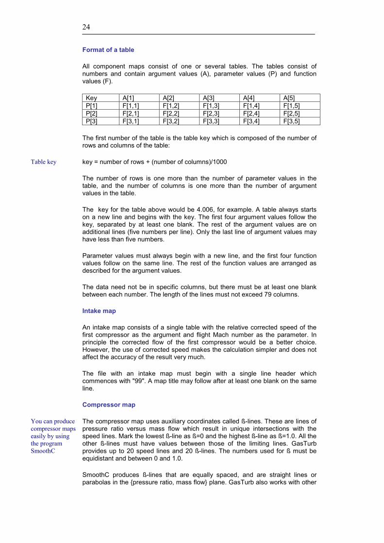
Format of a table
All component maps consist of one or several tables. The tables consist of numbers and contain argument values (A), parameter values (P) and function values (F).
Key A[1] A[2] A[3] A[4] A[5] P[1] F[1,1] F[1,2] F[1,3] F[1,4] F[1,5] P[2] F[2,1] F[2,2] F[2,3] F[2,4] F[2,5] P[3] F[3,1] F[3,2] F[3,3] F[3,4] F[3,5]
The first number of the table is the table key which is composed of the number of rows and columns of the table:
key = number of rows + (number of columns)/1000
The number of rows is one more than the number of parameter values in the table, and the number of columns is one more than the number of argument values in the table.
The key for the table above would be 4.006, for example. A table always starts on a new line and begins with the key. The first four argument values follow the key, separated by at least one blank. The rest of the argument values are on additional lines (five numbers per line). Only the last line of argument values may have less than five numbers.
Parameter values must always begin with a new line, and the first four function values follow on the same line. The rest of the function values are arranged as described for the argument values.
The data need not be in specific columns, but there must be at least one blank between each number. The length of the lines must not exceed 79 columns.
Intake map
An intake map consists of a single table with the relative corrected speed of the first compressor as the argument and flight Mach number as the parameter. In principle the corrected flow of the first compressor would be a better choice. However, the use of corrected speed makes the calculation simpler and does not affect the accuracy of the result very much.
The file with an intake map must begin with a single line header which commences with "99". A map title may follow after at least one blank on the same line.
Compressor map
The compressor map uses auxiliary coordinates called ß-lines. These are lines of pressure ratio versus mass flow which result in unique intersections with the speed lines. Mark the lowest ß-line as ß=0 and the highest ß-line as ß=1.0. All the other ß-lines must have values between those of the limiting lines. GasTurb provides up to 20 speed lines and 20 ß-lines. The numbers used for ß must be equidistant and between 0 and 1.0.
SmoothC produces ß-lines that are equally spaced, and are straight lines or parabolas in the pressure ratio, mass flow plane. GasTurb also works with other
Table key
You can produce compressor maps easily by using the program SmoothC

25
types of auxiliary coordinates. The numbers used for ß, however, must be equidistant and between 0 and 1.
In GasTurb the ß-lines need not be spaced equally in the pressure ratio, mass flow plane. If the ß-lines are not of the type that SmoothC produces, then GasTurb will not indicate precise information about surge margin and peak efficiency when you move the design point in a map with your mouse.
The detailed compressor map format is as follows. On the first line of a map data file there must be the number 99 followed by a blank. After that an arbitrary text - the map header line - may follow on the same line. On the second line the Reynolds number correction factors on efficiency are given in the following form:
Reynolds: RNI=x1 f = y1 RNI = x2 f = y2
The Reynolds number index is defined as
farT
farT
ref
ref
ref
ref
TTPP
RNI,
0,
//
µµ ==
where µ stands for dynamic viscosity and far for the fuel-air-ratio. Reference conditions are Pref=101.325kPa and Tref=288.15K.
In the figure the following numbers are used for illustration:
RNI = x1 = 0.1 f = y1 = 0.95 RNI = x2 = 1 f = y2 = 1
The efficiency correction factor is interpolated linearly over the logarithm of RNI. As RNI decreases the correlation is extrapolated if required. For RNI>x2 the efficiency correction factor remains constant and equal to y2.
From the efficiency correction factor there is a mass flow correction factor derived such that the mass flow correction is assumed to be half of the efficiency correction. For example, when efficiency is corrected using the factor 0.96, mass flow will be corrected with the factor 0.98.
On the third line of the compressor map data file GasTurb expects the keyword Mass Flow. On the following line the table for corrected mass flow has to start. The first number on this line is the table key derived from the number of speed lines and the number of ß-lines in the map:
Reynolds correction

26
key = (number of speed lines + 1) + (number of ß-lines +1)/1000
If there are 10 speed lines and 15 ß-lines, for example, the table key must be 11.016. After the table key the first four ß-values must follow. On the next lines follow the rest of the ß-values, five numbers on each line. The last line containing ß-values may have less than five numbers. Remember that the ß-values must be equidistant and between 0 (first ß-value) and 1.0 (last ß-value).
Then the speed value for the first speed line begins a new line. After that the first four mass flow numbers follow. The rest of the mass flow data for the first speed line appear on the following lines. Apart from the last line there must always be five numbers on each line. The rest of the speed lines (GasTurb can handle a maximum of 20 speed lines per map) must follow in an ascending order of speed.
The keyword Efficiency marks the start of the efficiency data. The sequence and the format of the data follow the same pattern as the one described for the corrected mass flow. Pressure ratio is the keyword for the third table of a compressor map.
The surge line completes a compressor map file. The keyword for the table is Surge Line. The surge pressure ratio is given as a function of the corrected mass flow. Note that you must store the data (up to 20 data points) in an ascending order of mass flow.
Propeller map
For the propeller maps auxiliary coordinates are also used. These maps are defined in the power coefficient, advance ratio plane. The map information is contained in two tables both with ß being the argument and advance ratio being the parameter. The propeller efficiency is the function value of the first table and the power coefficient is the function value of the second. Instead of the Reynolds correction information there must be a blank line in the file. The ß-values must be equidistant, beginning with ß=0 and ending with ß=1.0.
The static performance of the propeller completes the map. It is stored in the same format as a surge line and gives the ratio of thrust coefficient over power coefficient as a function of power coefficient. The keyword for this type of table is Static Performance.
Turbine map
The turbine map also uses ß-lines. They are defined in the pressure ratio,corrected speed plane. In two tables the pressure ratios for ß=0 and ß=1 are tabulated as a function of corrected speed. In two further tables, mass flow and efficiency are stored in the same way as the compressor maps, with corrected speed as parameter and ß as argument. The ß-values must be equidistant, beginning with ß=0 and ending with ß=1.
1.4.3. Map scaling example
Let us take the compressor map of a turbojet to explain the procedure. We may calculate the design point with the following properties, for example:
Corrected Mass Flow (W√ΘR/δ)dp 90.0 Pressure Ratio (P3/P2)dp 9.0 Efficiency ηdp 0.85
You can produce turbine maps easily by using the program SmoothT

27
The corrected spool speed of the design point is taken as a reference in all off-design calculations. It holds by definition:
Corrected Speed (N√ΘR)dp 1.000
For off-design calculations, the design point must be correlated with the map. This means that one point in the map has to be a reference point (subscript R,map) the design point (subscript dp) is matched with. As a default, the reference point is defined to be at ßR,map=0.5 and N/√ΘR,map=1.0. However, ßR,map and N/√ΘR,map can be modified easily either by using the mouse or by entering numbers. Using ßR,map=0.5 and N/√ΘR,map=1.0 along with the standard map HPC01.MAP yields
Corrected Mass Flow (W√ΘR/δ)R,map 33.48423 Pressure Ratio (P3/P2)R,map 8.311415 Efficiency ηR,map 0.860100
Note that for reading these values from the map tables a linear interpolation between ß=0.47368 and ß=0.52632 is required. The value read from the map tables needs to be corrected for Reynolds number effects with the terms fη,RNI and fW,RNI to be comparable with the design point efficiency ηdp:
RNImapRmapdp f ,,, * ηηη =
RNIWmapRRmapdpR fWW ,,, *)/()/( δδ Θ=Θ
Now, the map scaling factors can be calculated (assuming fη,RNI=0.99 and consequently fW,RNI =0.995):
70134.2*)/(
)/(
,,
=Θ
Θ=
RNIWmapRR
dpRMass fW
Wf
δδ
99824.0* ,,
==RNImapR
dpEff ff
ηηη
09418.11)/(
1)/(
,23
23/ 23
=−
−=
mapR
dpPP PP
PPf
0.11
,
==mapR
Speed Nf
These map scaling factors are applied to all the numbers in the map. The result is that after the scaling procedure the map will be in line with the design point. When off-design point data are plotted on the compressor map, then the map will be shown in its scaled form.
For good simulations you should always use the best maps available. Scaling a single-stage fan map to a pressure ratio of 10 would certainly not be a reasonable approach. Selecting a representative map is the responsibility of the user of GasTurb. The program cannot keep the user from using unrepresentative component maps.
Reynolds correction

28
1.4.4. Input data for off-design simulations
The input data selection screen for off-design calculations needs some explanation. If the input of Flight condition is selected, then the first few items on the screen are altitude, the deviation from ISA standard day ambient temperature at that altitude, relative humidity and the flight Mach number. Select the Ground input mode when simulating gas turbines for power generation; in this mode you can specify inlet total pressure and temperature, relative humidity and ambient pressure.
The engine installation definition consists of intake pressure ratio, various bleed options and power offtake for customer purposes.
Depending on the type of engine being simulated the Reheat Selection Switch may also be shown. Depending on the switch setting these data may or may not be needed for the calculation.
You can select the engine operating condition either by specifying the relative high-pressure spool speed ZXN or by setting the burner exit temperature ZT4. Note that the operating condition is also influenced by the limiter settings.
Some of the input quantities are marked as estimated values. Normally you need not bother about them. If the iteration does not converge you should try to modify them to get better starting values for the off-design iteration.
After the iteration variables there is the input for the pressure and the temperature flow distortion. Note that the number of iteration variables changes with the type of distortion.
The group of off-design input data on the page with the heading Modifiers allows you to study changes of turbine flow capacity and nozzle area for the simulation of variable geometry. You can also modify the compressor flow capacity and the efficiency of the components to study deterioration effects, for example.
During off-design calculations the number of input data parameters is limited because the basic behavior of the engine is fixed with the engine cycle design point. Duct pressure losses, for example, are specified for the cycle design point and will vary with corrected flow at partload. Therefore you normally need not enter any data for duct pressure losses during off-design calculations, and you will not find the duct pressure losses among the off-design input data.
However, you might be interested in the effect of increased pressure losses at off-design in special cases. For this purpose, you can redefine your off-design input quantities with the corresponding option from the menu Define | Input Quantities.
1.4.5. Variable compressor geometry
On the notebook page Variable Geometry you can select a compressor with variable geometry. You could, for example, select variable geometry for the fan of an engine with a very high bypass ratio. Alternatively, you could test this feature with the booster of a turboprop engine.
At the design point the nominal setting of the variable geometry is by definition 0°. Any deviation from this setting will affect mass flow, pressure ratio and efficiency. You have to define the following influence coefficients before you can simulate variable geometry for a compressor:

29
[ ][ ]°
=VGWaVG δ
δ %
[ ][ ]°
−=VGPPbVG δ
δ %)1/(
[ ][ ]%%
VGcVG δ
δη=
The mass flow and the term pressure ratio - 1 will vary proportionally to the variable geometry setting δVG, which is an input quantity. The efficiency correction is done using a quadratic function. The program will correct the efficiency according to the following formula:
−=
1001* 2 VG
mapcVGδηη
Any deviation from the nominal setting will thus cause a loss in efficiency. The values for mass flow and pressure ratio will rise for positive δVG values and decrease for negative δVG values.
1.4.6. Limiters
The maximum power available from a given engine depends on several limits such as the maximum spool speed, maximum temperature and maximum pressure. Which limiter is active depends, among other things, on the flight condition, the amount of power offtake and bleed air offtake. The program can use several limiters simultaneously. The solution found will be a cycle with at least one limit being reached.
You can switch on the limiters individually. Note that all mechanical and aerodynamic speed limits are percentages of the design point data. Furthermore, you can define a composed value as an additional limit. Use this option for specifying a certain thrust or fuel flow, or any other computed quantity.
For a better approximation of real engine control systems, you can introduce control schedules into your simulation. With a control schedule you can make limiters dependent on the flight conditions. In many engine control systems the turbine exit temperature T5 is a function of inlet temperature T2, for example.
Besides limiter schedules you can also define other schedules. For example, a nozzle area trim can be made a function of corrected spool speed. The permissible parameter combinations depend on the engine configuration.
1.4.7. Reheat (Afterburning)
A reheated cycle is calculated in two steps. First, the program finds a dry operating point. After convergence the necessary reheat fuel flow for the desired T7 will be calculated. A new nozzle throat area follows from the revised nozzle inlet conditions.

30
There are thus two nozzle throat areas in a reheated cycle calculation. One is the equivalent dry nozzle area, which determines the turbomachinery operating conditions. The other one is the actual nozzle throat area.
1.4.8. Operating line
An operating line is a series of points starting with the last calculated single off-design point. Consecutive points are obtained by decreasing the high-pressure spool speed in steps of 0.025. A series of reheat partload points can also be an operating line. Starting from the design point value the reheat exit temperature is decreased in steps of 100K. Note that the operating point in the turbomachinery component maps is the same for all points of a reheat operating line. You can calculate reheat for off-design conditions only if your design point was calculated with the reheat switched on.
To control the compressor surge margin you can select an automatic handling bleed. This bleed discharges some of the compressed air into the bypass duct or overboard. You can thus lower the operating line of the compressor and avoid a surge. The automatic handling bleed will be modulated between the two switch-points that you specify.
1.4.9. Off-design parametric study
Instead of creating an operating line with several values for the high-pressure spool speed you can also produce a series of points with different amounts of power offtake and customer bleed air extraction, for example. This is initiated with the same input scheme as for design point parameter studies.
The operating lines are also shown in the component maps. Note that the efficiency contours in the maps are valid for RNI=1 and delta efficiency=0 only. The efficiencies calculated in the cycle are often different because of Reynolds number corrections. So do not be surprised if you fail to find the same efficiency along the operating line in the HPC map and in the plot HPC Efficiency, HPC Mass Flow.
1.4.10. Calculation of a flight envelope
After specifying one or several limiters or control schedules you can calculate a series of points with different altitudes throughout a flight envelope. A flight envelope always starts at sea level and extends to the specified altitude. Two limiting speed values are entered as equivalent air speed EAS. This is the speed at which the airplane must fly at some altitude other than sea level to produce the same dynamic pressure as at sea level. EAS is traditionally measured in knots and differs from the true airspeed by the square root of the density ratio ρ/ρ0.
0/* ρρVEAS =
There are four speed limits that define the flight envelope. For altitudes lower than 3048 m (10000 ft) the flight envelope extends to zero speed. Above this altitude the limit of the flight envelope is the minimum Equivalent Air Speed. The maximum speed is described by both a maximum EAS and by a maximum Mach number (lowest is used).
A simplified definition of the flight envelope yields the engine performance for equal steps in altitude and Mach number.
Automatic bleed

31
You can calculate up to 30 altitude levels and up to 30 speed values in a flight envelope. Select many points if you are interested in the transition between the different limiters. Note that in the graphs of flight envelope data the calculated points are connected linearly. This is because the switchover from one limiter to another can result in sharp bends in the curves. If the program were to use splines to connect the points there, which is done in other graphs produced by GasTurb, the sharp bends would be hidden.
The first point calculated is always sea level static. This point must converge; otherwise, the calculation will stop with a corresponding message.
As the first graph you are offered a plot of the flight envelope in which you can see which limiter is active at any altitude and Mach number combination.
1.4.11. Off-design effects
There can be a big difference in the results found for small changes in compressor efficiency between cycle design point calculations and those for off-design. In the latter case all the operating points are moving around in their component maps and it might happen that decreasing the quality of a component improves thrust!
Note also that the effects can depend very much on the flight condition and on the engine operating conditions. Effects for constant thrust differ from those for constant burner exit temperature or constant speed.
Be careful when looking at the results especially in case of surge margin. The differences are presented as a percentage of the original value. Surge margin is already a value expressed in terms of a percentage, typically 25%. When an effect causes a reduction in surge margin by 2.5% then you will find in the table on the screen the value 10, since 2.5% is 10% of the original value.
1.4.12. Off-design Monte Carlo simulation
With the Monte Carlo method you can simulate the performance variations that result from random changes of the component behaviour due to manufacturing and assembly tolerances in a series production of engines. See which component production and control system tolerances you can afford without getting an excessive scatter in pass-off thrust or specific fuel consumption.
The random distributions for all input data are independent of each other. There is one exception to this rule: a compressor with an efficiency level lower than the mean value is assumed to also have a corrected flow at a given speed, which is lower than average.
1.4.13. Mission calculations
Often one has to look in detail at many different off-design conditions of a gas turbine. To do this easily, you may define a mission. You can combine up to 30 different operating conditions in a list of mission points.
When you start the calculation, then all points in this list will be calculated in one run. The results are presented in a summary table. You may rearrange the sequence of the lines in that table to put those items first that are of most interest for your specific problem.
Effects on surge margin

32
Besides the summary table you can also get detailed information for every single point. Furthermore, all points of a mission will be plotted in the component maps.
1.4.14. Off-design constraints in a cycle design optimisation
The sizing of an engine for a subsonic transport aircraft is generally done for an aerodynamic design point at high altitude. For such a flight condition one normally gets high Mach numbers at the compressor inlet, but rather moderate turbine inlet temperatures.
The maximum turbine inlet temperature will occur at hot day take-off conditions. From a cycle design point of view this is an off-design case.
During a cycle design optimization exercise you can take constraints from one off-design point into account. Define a mission with one single point for that purpose before initiating the optimization. Then, for each of the seven constraints you may choose whether it applies to the design point or to the off-design point.
1.4.15. Test analysis by synthesis
The conventional test analysis makes no use of information that is available from component rig tests, for example. It will give no information about the reason why a component behaves badly. A low efficiency for the fan may be either the result of operating the fan at aerodynamic overspeed or a poor blade design. To improve the analysis quality in this respect is the aim of the Analysis by Synthesis (AnSyn). This method is also known as model based engine monitoring.
When doing analysis by synthesis a model of the engine is automatically matched to the test data. Applying scaling factors to the component models so that the measured values and the model values come into agreement does this. An efficiency scaling factor greater than one indicates, that the component performs better than predicted, for example.
The mass flow through an engine can be directly measured or analyzed from various other measurements. For a single spool turboshaft, for example, the compressor mass flow can be calculated from the turbine flow capacity or from the measured exit temperature T5 if fuel flow is known.
For each engine configuration GasTurb offers a selection of mass flow analysis methods. It depends on the accuracy of the sensors which method provides the most reasonable test analysis result. Check the effects of sensor errors on the analysis result with the menu option Task|Effects
Mass flow analysis

33
2. Theory The following chapters describe the calculations done for some characteristic engine types. You only need to read the appropriate section for your engine type, since the chapters do not depend on each other. The nomenclature used in the following chapters is consistent with the nomenclature in the source code.
After the general description there are chapters that provide the details of the calculations.
2.1. Description of some typical engine configurations
2.1.1. Single spool turbojet
The calculation starts with the intake. The altitude, flight Mach number and ∆TISA yield the ambient temperature and pressure, the flight velocity and the total engine inlet conditions T1 and P1. The pressure at the compressor inlet can be easily calculated from the input value of the intake pressure ratio P2/P1 or from the value read from the intake map.
In the case of design calculations the total corrected engine mass flow W2√ΘR,2/δ2 is an input. W2 can be derived easily.
In the case of off-design the relative corrected compressor spool speed is
Design
C
C
relcorrC
TRN
TRN
N
=
2
2,,
*
*
The compressor map is read with help of the relative corrected speed and the auxiliary map coordinate ßC. This yields the standard day corrected mass flow W2√ΘR,2/δ2, the isentropic efficiency η23, the pressure ratio P3/P2 and the surge margin. NC and ßC are estimated values in an off-design calculation. W2 can easily be derived from W2√ΘR,2/δ2, T2 and P2.
To perform a simulation of inlet flow distortion as well as to study the transient behavior one needs some engine geometry data. They will be calculated if you select Compressor Design. Then W2, T2, P2, the blade tip velocity, the inlet hub/tip radius ratio and the axial Mach number are used to calculate the tip diameter, the relative and circumferential Mach numbers, and the angular velocity.
For the description of the inlet flow distortion the static quantities in the aerodynamic interface plane are required. The flow area is derived from the compressor tip diameter.
Now we can calculate the compression process, which yields the compressor exit temperature T3, as well as the specific work dH23.
Compressor map
Distortion and transient simulations
Aerodynamic interface plane

34
Next we look at the internal air system. The turbine cooling air mass flow is
=
2
,2, *
WW
WW TClTCl
This amount of cooling air is assumed not to do any work; it is mixed with the main gas stream behind the turbine. The nozzle guide vane (NGV) cooling air mass flow is calculated in a similar manner:
=
2
,2, *
WW
WW NGVClNGVCl
The NGV cooling air is mixed with the main stream at station 41 upstream of the rotor(s), consequently this amount of air does work in the turbine.
2 3 441
5 8661
7 9
NGVCool.
OverboardBleed
HandlingBleed
HPTCooling
31
TJetRHCDPPT.WMF GasTurb
The overboard bleed mass flow can be entered as a linear combination of a relative and an absolute amount
2,2
1,2 * Bld
BldBld W
WW
WW +
=
The work done on the overboard bleed is:
23*dHfdH BldBld =
In an operating line calculation and during the simulation of the transient behavior you can select the handling bleed to be switched automatically. The bleed valve is closed when the relative corrected compressor speed is higher than NC,corr,rel,2. It will be open if the corrected speed is lower than NC,corr,rel,1. If the corrected spool
Internal air system
Customer bleed air
Automatic handling bleed

35
speed is between these boundaries then the handling bleed flow is interpolated linearly:
−−
−
=
1,,,2,,,
1,,,,,
max22 1**
relcorrCrelcorrC
relcorrCrelcorrCHdlBldHdlBld NN
NNWW
WW
The NGV and turbine rotor cooling air as well as the handling bleed air is compressed fully; the specific power required for this is dH23. The mass flow at the compressor exit W3 is the flow without the inter-stage bleed that is not fully compressed (an inter-stage bleed is modeled with fBld<1):
BldWWW −= 23
Between stations 3 and 31 the fully compressed bleeds are taken off:
HdlBldTClNGVCl WWWWW −−−= ,,331
In design calculations the burner pressure ratio P4/P3 is given, whereas in off-design calculations it is derived from the corrected flow and the design point pressure ratio. The amount of fuel is calculated from the required fuel-air-ratio, which in turn depends on burner pressure, inlet temperature, humidity and temperature rise.
)(*/23134 OHf WWfarW −= η
The burner exit flow is W4=W31+Wf, and the turbine nozzle guide vane exit flow is W41=W4+WCl,NGV. The fuel-air-ratio far41 is
OHf
f
WWWW
far241
41 −−=
Now it is possible to calculate the enthalpy corresponding to the Stator Outlet Temperature (SOT) or Rotor Inlet Temperature (RIT) of the turbine:
413,4441 /)**( WHWHWH NGVCl+=
The power delivered by the turbine is a product of W41 and the specific power dH41,49. The energy balance with all power requirements, including the customer power offtake PWX, is given by
mech
BldBld
WPWXdHWdHW
dHη***
41
23349,41
++=
If Turbine Design is selected, then the isentropic efficiency is calculated, otherwise, it is given as an input property. In off-design simulations the efficiency is read from the turbine map.
The relative corrected turbine speed is
Burner

36
Design
C
C
relcorrT
TRN
TRN
N
=
41
41,,
*
*
The turbine efficiency and the corrected flow are read from the map with the known relative corrected spool speed and the auxiliary coordinate ßT. The efficiency can be modified in off-design simulations by a tip clearance correction term, which is a function of the relative mechanical spool speed NC:
CCclearancetip NN
δδηη *)1( −=∆
From the specific work dH41,49 and the efficiency we can calculate P49 = P5 and the turbine rotor exit temperature T49. Then the turbine rotor cooling air is added:
TClWWW ,415 +=
The turbine exit enthalpy H5 is calculated on the basis of the energy balance:
5
,3414141495
**),,(W
WHWwarfarThH TCl+
=
The fuel air ratio comes from
OHf
f
WWWW
far25
5 −−=
In design calculations the turbine exit duct pressure ratio P6/P5 is given, while in off-design simulations it is calculated as a function of corrected flow.
If the engine has no reheat system, then the nozzle inlet conditions are the same as in station 6. Otherwise, a nozzle cooling air flow is detracted from the mass flow W6 =W5 to yield the reheat inlet mass flow W61:
−=
6
,6661 *
WW
WWW NozCl
Then the fuel-air-ratio far7 is calculated from the specified reheat exit temperature T7. Reheat fuel flow is then
−= 1*
6
7, far
farWW fRHf
The total reheat exit mass flow amounts to W7=W61+Wf,RH. The fundamental pressure loss caused by the heat addition will then be calculated. The correlations of the Rayleigh line, i.e., heat addition in a pipe with constant area, are used. The inlet Mach number for this calculation is M6.
Reheat
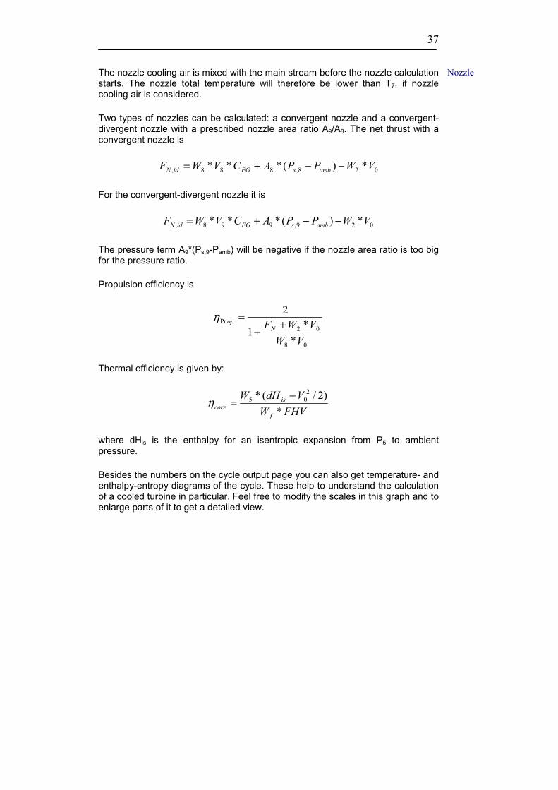
37
The nozzle cooling air is mixed with the main stream before the nozzle calculation starts. The nozzle total temperature will therefore be lower than T7, if nozzle cooling air is considered.
Two types of nozzles can be calculated: a convergent nozzle and a convergent-divergent nozzle with a prescribed nozzle area ratio A9/A8. The net thrust with a convergent nozzle is
028,888, *)(*** VWPPACVWF ambsFGidN −−+=
For the convergent-divergent nozzle it is
029,998, *)(*** VWPPACVWF ambsFGidN −−+=
The pressure term A9*(Ps,9-Pamb) will be negative if the nozzle area ratio is too big for the pressure ratio.
Propulsion efficiency is
08
02Pr
**
1
2
VWVWFN
op ++
=η
Thermal efficiency is given by:
FHVWVdHW
f
iscore *
)2/(* 205 −
=η
where dHis is the enthalpy for an isentropic expansion from P5 to ambient pressure.
Besides the numbers on the cycle output page you can also get temperature- and enthalpy-entropy diagrams of the cycle. These help to understand the calculation of a cooled turbine in particular. Feel free to modify the scales in this graph and to enlarge parts of it to get a detailed view.
Nozzle

38

39
2.1.2. Single spool turboshaft
The calculation starts with the intake. The altitude, flight Mach number and ∆TISA yield the ambient temperature and pressure, the flight velocity and the total engine inlet conditions T1 and P1. The pressure at the compressor inlet can be easily calculated from the input value of the intake pressure ratio P2/P1 or from the value read from the intake map.
In the case of design calculations the total corrected engine mass flow W2√ΘR,2/δ2 is an input. W2 can be derived easily.
In the case of off-design the relative corrected compressor spool speed is
Design
C
C
relcorrC
TRN
TRN
N
=
2
2,,
*
*
The compressor map is read with help of the relative corrected speed and the auxiliary map coordinate ßC. This yields the standard day corrected mass flow W2√ΘR,2/δ2, the isentropic efficiency η23, the pressure ratio P3/P2 and the surge margin. NC and ßC are estimated values in an off-design calculation. W2 can easily be derived from W2√ΘR,2/δ2, T2 and P2.
To perform a simulation of inlet flow distortion as well as to study the transient behavior one needs some engine geometry data. They will be calculated if you select Compressor Design. Then W2, T2, P2, the blade tip velocity, the inlet hub-tip radius ratio and the axial Mach number are used to calculate the tip diameter, the relative and circumferential Mach numbers, and the angular velocity.
For the description of the inlet flow distortion the static quantities in the aerodynamic interface plane are required. The flow area is derived from the compressor tip diameter.
Now we can calculate the compression process, which yields the compressor exit temperature T3, as well as the specific work dH23.
Next we look at the internal air system. The turbine cooling air mass flow is
=
2
,2, *
WW
WW TClTCl
This amount of cooling air is assumed not to do any work; it is mixed with the main gas stream behind the turbine. The nozzle guide vane (NGV) cooling air mass flow is calculated in a similar manner:
Compressor map
Distortion and transient simulations
Aerodynamic interface plane
Internal air system

40
=
2
,2, *
WW
WW NGVClNGVCl
The NGV cooling air is mixed with the main stream at station 41 upstream of the rotor(s), consequently this amount of air does work in the turbine.
The overboard bleed mass flow can be entered as a linear combination of a relative and an absolute amount
2,2
1,2 * Bld
BldBld W
WW
WW +
=
The work done on the overboard bleed air is:
23*dHfdH BldBld =
In an operating line calculation and during the simulation of the transient behavior you can select the handling bleed to be switched automatically. The bleed valve is closed if the relative corrected compressor speed is higher than NC,corr,rel,2. It will be open if the corrected speed is lower than NC,corr,rel,1. If the corrected spool speed is between these boundaries then the handling bleed flow is interpolated linearly:
−−
−
=
1,,,2,,,
1,,,,,
max22 1**
relcorrCrelcorrC
relcorrCrelcorrCHdlBldHdlBld NN
NNWW
WW
2 3 4
41 86
5
35
7
31
HPTCooling
NGVCool.
OverboardBleeds
HandlingBleed
TJetExPPT.WMF GasTurb
The NGV and turbine rotor cooling air as well as the handling bleed air is compressed fully; the specific power required for this is dH23. The mass flow at
Customer bleed air
Automatic handling bleed

41
the compressor exit W3 is the flow without the inter-stage bleed that is not fully compressed (an inter-stage bleed is modeled with fBld<1):
BldWWW −= 23
Between stations 3 and 31 the fully compressed bleeds are taken off:
HdlBldTClNGVCl WWWWW −−−= ,,331
However, when the engine is equipped with a heat exchanger then the nozzle guide vane cooling air is not subtracted from W31 because WCl,NGV is taken from the flame tube cooling air:
HdlBldTCl WWWWW −−== ,33531
If there is no heat exchanger then T35 equals T3 and P35 equals P3. If a turboshaft with a heat exchanger is to be calculated, an iteration must be initiated. The cold-side exit temperature of the heat exchanger, T35, is estimated to be T3+300K. The pressure loss from station 3 to station 35 is calculated differently for design and off-design. In the first case the pressure ratio P35/P3 is given as input, whereas in the second case the losses depend on the corrected flow.
The pressure loss in the burner is calculated in the same way as the heat exchanger loss: in design calculations the pressure ratio P4/P35 is given, whereas in off-design calculations it is a function of the corrected flow and the design point pressure ratio.
The amount of fuel is calculated from the required fuel-air-ratio, which in turn depends on burner pressure, inlet temperature, humidity of the incoming air and temperature rise. Water or steam injection into the burner can be considered also.
)(*/23534 OHf WWfarW −= η
The burner exit flow is W4=W35+(SFR+WFR)*Wf, and the turbine nozzle guide vane exit flow is W41=W4+WCl,NGV. The fuel-air-ratio far41 is
OHf
f
WWWW
far241
41 −−=
Now it is possible to calculate the enthalpy corresponding to the Stator Outlet Temperature (SOT) or Rotor Inlet Temperature (RIT) of the turbine:
4135,4441 /)**( WHWHWH NGVCl+=
In a design calculation you can specify the nozzle pressure ratio P6/Pamb. From P4, ambient pressure, turbine exit duct pressure ratio P6/P5 and nozzle pressure ratio, you can calculate the turbine pressure ratio P4/P5. From mass flow W41, efficiency and pressure ratio, the turbine power follows. The shaft power delivered will be
CTmechSD PWPWPW −= *η
Heat exchanger
Burner
Turbine

42
For off-design calculations the shaft power can be prescribed via the following formula (The values for c and n in this formula are input data):
nDesignSDSD PWcPW ,*=
If Turbine Design is selected then the isentropic efficiency is calculated, otherwise, it is given as an input property. In off-design simulations the efficiency is read from the turbine map.
The relative corrected turbine speed is
Design
C
C
relcorrT
TRN
TRN
N
=
41
41,,
*
*
The turbine efficiency and the corrected flow are read from the map with the known relative corrected spool speed and the auxiliary coordinate ßT. The efficiency can be modified in off-design simulations by a tip clearance correction term, which is a function of the relative mechanical spool speed:
CCclearancetip NN
δδηη *)1( −=∆
The turbine exit conditions, i.e., T49 and P5, can now be calculated using the pressure ratio and efficiency. The cooling air will be mixed in the next step:
TClWWW ,415 +=
OHf
f
WWWW
far25
5 −−=
5
49493,5
**W
HWHWH TCl +
=
The turbine exit duct pressure ratio can be found in the usual way. During off-design calculations the turbine exit flow angle can vary considerably. If you want to model the pressure losses as a function of flow angle, then you must select Turbine Design for the turbine. That provides the area A5, the mean diameter of the turbine, and the blade exit flow angle, which is assumed to be equal to the blade metal angle ßBlade
During off-design the axial flow velocity can be found approximately from
55
555, *
**PATRW
Vax =
Turbine exit duct

43
The use of the total quantities T5 and P5 instead of the static quantities Ts5 and Ps5 does not matter very much, since the Mach number is usually low behind the turbine. The absolute turbine exit flow angle can be found using the circumferential speed U5 and the blade metal angle.
5,
5tantanax
Blade VU
−= βα
You can input the geometric angle of the struts in the turbine exit duct. If there is zero incidence at the struts leading edge, then the pressure losses will be minimal. For other flow angles there will be an additional pressure loss due to the incidence of the flow direction relative to the strut. To describe this a loss factor finc is calculated
)(*cos strutc
incf αα −=
The exponent c in this formula allows one to adapt the loss characteristics as required. The pressure loss of the turbine exit duct is then
incLossMinDesignR
fPP
WPWRT
PP
*1**
**15
6
2
,,55
55
5
6
−
−=
If a heat exchanger is installed then its hot side pressure losses will be either given (design case) or calculated (off-design) as a function of the corrected flow.
The heat exchanger exit temperature T7 is derived from its effectiveness, which is an input property:
( )3667 ** TTCC
TTh
cex −−= η
with
[ ] 2/)()(* 35331 TcTcWC ppc +=
and
[ ] 2/))(()(* 335666 TTTcTcWC pph −−+=
Until now only an estimated value has been used for the cold side heat exchanger exit temperature T35. We must check whether this value satisfies the heat balance equation:
)(*)(* 76633531 HHWHHW −=−
As long as this equation is not satisfied, an improved value for T35 has to be estimated, and the calculations must be restarted at the burner inlet.
Heat exchanger

44
Without a heat exchanger the turbine exit duct conditions are identical to the exhaust diffuser inlet conditions. You have to include the pressure losses of the exhaust diffusor into the pressure losses of the turbine exhaust diffusor.
For engines with heat exchanger the hot side pressure losses of the heat exchanger must include the exhaust diffusor losses.
Only a few additional calculations remain now:
Thermal efficiency
FHVWPW
f
SDtherm *
=η
Core efficiency
FHVWVdHW
f
iscore *
)2/(* 205 −
=η
The enthalpy dHis is calculated assuming an isentropic expansion from station 5 to ambient pressure.
If the engine is configured as a turboprop then the total thrust is the sum of propeller thrust and residual thrust. The details of the propeller calculations are described in the component simulation chapter. The residual thrust is
0288 *** VWCVWF FGN −=
You can select an enthalpy-entropy or a temperature-entropy diagram as a graph. It will show all of the thermodynamic stations of the cycle. Some stations are often very close to each other. This makes it difficult to distinguish among all of the details in the original scale. If you are interested in a special part of the cycle diagram, you should enlarge the relevant section.
Turboprop

45
2.1.3. Two-spool turboshaft, turboprop
The calculation starts with the intake. The altitude, flight Mach number and ∆TISA yield the ambient temperature and pressure, the flight velocity and the total engine inlet conditions T1 and P1. The pressure at the compressor inlet can be easily calculated from the input value of the intake pressure ratio P2/P1 or from the value read from the intake map.
In the case of design calculations the total corrected engine mass flow W2√ΘR,2/δ2 is an input. W2 can be derived easily.
In the case of off-design the relative corrected compressor spool speed is
Design
C
C
relcorrC
TRN
TRN
N
=
2
2,,
*
*
The compressor map is read with help of the relative corrected speed and the auxiliary map coordinate ßC. This yields the standard day corrected mass flow W2√ΘR,2/δ2, the isentropic efficiency η23, the pressure ratio P3/P2 and the surge margin. NC and ßC are estimated values in an off-design calculation. W2 can easily be derived from W2√ΘR,2/δ2, T2 and P2.
To perform a simulation of inlet flow distortion as well as to study the transient behavior one needs some engine geometry data. They will be calculated if you select Compressor Design. Then W2, T2, P2, the blade tip velocity, the inlet hub-tip radius ratio and the axial Mach number are used to calculate the tip diameter, the relative and circumferential Mach numbers, and the angular velocity.
For the description of the inlet flow distortion the static quantities in the aerodynamic interface plane are required. The flow area is derived from the compressor tip diameter.
Now we can calculate the compression process, which yields the compressor exit temperature T3, as well as the specific work dH23.
Next we look at the internal air system. The high-pressure turbine (HPT) cooling air mass flow is
=
2
,2, *
WW
WW HPTClHPTCl
This amount of cooling air is assumed not to do any work; it is mixed with the main gas stream downstream of the turbine. The nozzle guide vane (NGV) cooling air mass flow is calculated in a similar manner:
Compressor map
Distortion and transient simulations
Aerodynamic interface plane
Internal air system
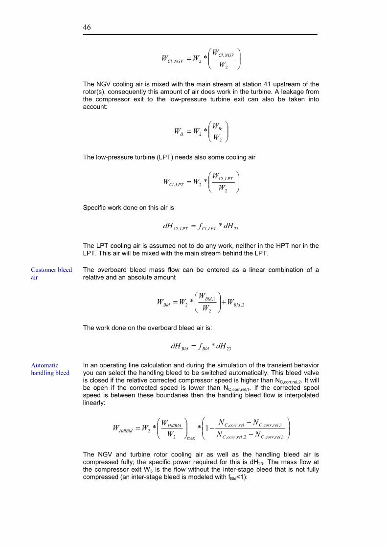
46
=
2
,2, *
WW
WW NGVClNGVCl
The NGV cooling air is mixed with the main stream at station 41 upstream of the rotor(s), consequently this amount of air does work in the turbine. A leakage from the compressor exit to the low-pressure turbine exit can also be taken into account:
=
22 *
WW
WW lklk
The low-pressure turbine (LPT) needs also some cooling air
=
2
,2, *
WW
WW LPTClLPTCl
Specific work done on this air is
23,, *dHfdH LPTClLPTCl =
The LPT cooling air is assumed not to do any work, neither in the HPT nor in the LPT. This air will be mixed with the main stream behind the LPT.
The overboard bleed mass flow can be entered as a linear combination of a relative and an absolute amount
2,2
1,2 * Bld
BldBld W
WW
WW +
=
The work done on the overboard bleed air is:
23*dHfdH BldBld =
In an operating line calculation and during the simulation of the transient behavior you can select the handling bleed to be switched automatically. This bleed valve is closed if the relative corrected compressor speed is higher than NC,corr,rel,2. It will be open if the corrected speed is lower than NC,corr,rel,1. If the corrected spool speed is between these boundaries then the handling bleed flow is interpolated linearly:
−−
−
=
1,,,2,,,
1,,,,,
max22 1**
relcorrCrelcorrC
relcorrCrelcorrCHdlBldHdlBld NN
NNWW
WW
The NGV and turbine rotor cooling air as well as the handling bleed air is compressed fully; the specific power required for this is dH23. The mass flow at the compressor exit W3 is the flow without the inter-stage bleed that is not fully compressed (an inter-stage bleed is modeled with fBld<1):
Customer bleed air
Automatic handling bleed

47
BldWWW −= 23
Between stations 3 and 31 the fully compressed bleeds are taken off:
HdlBldHPTClNGVCl WWWWW −−−= ,,331
2 3 4
41 845 65
44
35
7
31
HPTCooling
NGVCool.
OverboardBleeds
HandlingBleed
HP leak to LPT exit
GasTurbTShtExchPPT.WMF
LPT cooling
However, if the engine is equipped with a heat exchanger then the nozzle guide vane cooling air is not subtracted from W31 because WCl,NGV is taken from the flame tube cooling air:
HdlBldHPTCl WWWWW −−== ,33531
If there is no heat exchanger then T35 equals T3 and P35 equals P3. If a turboshaft with a heat exchanger is to be calculated, an iteration must be initiated. The cold-side exit temperature of the heat exchanger, T35, is estimated to be T3+300K. The pressure loss from station 3 to station 35 is calculated differently for design and off-design. In the first case the pressure ratio P35/P3 is given as input, whereas in the second case the losses depend on the corrected flow.
The pressure loss in the burner is calculated in the same way as the heat exchanger loss: in design calculations the pressure ratio P4/P35 is given, whereas in off-design calculations it is a function of the corrected flow and the design point pressure ratio.
The amount of fuel is calculated from the required fuel-air-ratio, which in turn depends on burner pressure, inlet temperature, humidity of the incoming air and temperature rise. Water or steam injection into the burner can be considered also.
)(*/23534 OHf WWfarW −= η
Heat exchanger
Burner

48
The burner exit flow is W4=W35+(SFR+WFR)*Wf and the turbine nozzle guide vane exit flow W41 equals W4+WCl,NGV. The fuel-air-ratio far41 is
OHf
f
WWWW
far241
41 −−=
Now it is possible to calculate the enthalpy corresponding to the Stator Outlet Temperature (SOT) or Rotor Inlet Temperature (RIT) of the turbine:
4135,4441 /)**( WHWHWH NGVCl+=
The power delivered by the turbine is a product of W41 and the specific power dH41,44. The energy balance with all power requirements, including the customer power offtake PWX, is given by
mech
BldBldLPTClLPTCl
WPWXdHWdHWdHW
dHη*
***
41
,,23344,41
+++=
If Turbine Design is selected then the isentropic efficiency is calculated, otherwise, it is given as an input property. In off-design simulations the efficiency is read from the turbine map.
The relative corrected turbine speed is
Design
C
C
relcorrHPT
TRN
TRN
N
=
41
41,,
*
*
The turbine efficiency and the corrected flow are read from the map with the known relative corrected spool speed and the auxiliary coordinate ßHPT. The efficiency can be modified in off-design simulations by a tip clearance correction term, which is a function of the relative mechanical spool speed:
CCclearancetip NN
δδηη *)1( −=∆
From the specific work dH41,44 and the efficiency we can calculate P43= P44 and the turbine rotor exit temperature T43. Then the turbine rotor cooling air is added: W45=W41+WCl,HPT. The LPT inlet enthalpy H45 is calculated using the energy balance:
45
,34141414345
**),,(W
WHWwarfarThH HPTCl+
=
The fuel air ratio comes from
High pressure turbine

49
OHf
f
WWWW
far245
45 −−=
Pressure losses in the inter-duct between both turbines can be calculated in several ways. For design calculations, when turbine efficiency is an input property, P45/P44 is a given quantity. If Turbine Design is selected and a value for the reference Mach number M44>0 is given, then the pressure loss will be adjusted to the actual Mach number level. If the reference Mach number is not given, then the input value of P45/P44 is used again. During off-design the losses vary with the corrected flow in the same way as in any duct.
Usually the low-pressure turbine (LPT) efficiency is an input value. Efficiency, however, can also be calculated in a turbine design calculation. The mechanical speed of the LPT is an input value. The pressure ratio of the turbine is given by P45 and
6
5
7
6
8
785 P
PPP
PP
PP
PPamb
amb=
Except P7/P8, which is set to 1.0 in this program, these pressure ratios are input data. P6/P7 is the heat exchanger hot side pressure ratio (equals 1.0 if no heat exchanger is present), and P6/P5 is the turbine exit duct pressure ratio.
In the case of off-design the relative corrected speed of the LPT is
Design
LPT
LPT
relcorrLPT
TRN
TRN
N
=
45
45,,
*
*
The operating point in the map is determined by the estimated value of the auxiliary coordinate, ßLPT, and the relative corrected speed. Both the corrected flow, W45,std, and the efficiency are read from the tables.
The LPT exit conditions, i.e., T49 and P5, can now be calculated using the pressure ratio and efficiency. The cooling and the leakage air will be mixed in the next step:
lkLPTCl WWWW ++= ,455
OHf
f
WWWW
far25
5 −−=
5
34945,,5
***W
HWHWHWH lkLPTClLPTCl ++
=
The turbine exit duct pressure ratio can be found in the usual way. During off-design calculations the turbine exit flow angle can vary considerably. If you want to model the pressure losses as a function of flow angle, then you must select
Turbine inter-duct
Low-pressure turbine
Turbine exit duct

50
Turbine Design for the LPT. That provides the area A5, the mean diameter of the low pressure turbine, and the blade exit flow angle, which is assumed to be equal to the blade metal angle ßBlade
During off-design the axial flow velocity can be found approximately from
55
555, *
**PATRW
Vax =
The use of the total quantities T5 and P5 instead of the static quantities Ts5 and Ps5 does not matter very much, since the Mach number is usually low behind the LPT. The absolute flow angle can be found using the circumferential speed U5 and the blade metal angle.
5,
5tantanax
Blade VU
−= βα
You can input the geometric angle of the struts in the turbine exit duct. If there is zero incidence at the struts leading edge, then the pressure losses will be minimal. For other flow angles there will be an additional pressure loss due to the incidence of the flow direction relative to the strut. To describe this a loss factor finc is calculated
)(*cos strutc
incf αα −=
The exponent c in this formula allows one to adapt the loss characteristics as required. The pressure loss of the turbine exit duct is then
incLossMinDesignR
fPP
WPWRT
PP
*1**
**15
6
2
,,55
55
5
6
−
−=
When a heat exchanger is installed then its hot side pressure losses will be either given (design case) or calculated (off-design) as a function of the corrected flow.
The heat exchanger exit temperature T7 is derived from the input value for its effectiveness:
( )3667 ** TTCC
TTh
cex −−= η
with
[ ] 2/)()(* 35331 TcTcWC ppc +=
and
[ ] 2/))(()(* 335666 TTTcTcWC pph −−+=
Heat exchanger

51
Until now only an estimated value has been used for the cold side heat exchanger exit temperature T35. We must check whether this value satisfies the heat balance equation:
)(*)(* 76633531 HHWHHW −=−
As long as this equation is not satisfied, an improved value for T35 has to be estimated, and the calculations must be restarted at the burner inlet.
Without a heat exchanger the turbine exit duct conditions are identical to the exhaust diffuser inlet conditions. You have to include the pressure losses of the exhaust diffusor into the pressure losses of the turbine exhaust diffusor.
For engines with heat exchanger the hot side pressure losses of the heat exchanger must include the exhaust diffusor losses.
Only a few additional calculations remain now:
Shaft power delivered
5,4545, ** dHWPW LmechSD η=
Thermal efficiency
FHVWPW
f
SDtherm *
=η
Core efficiency
FHVWVdHW
f
iscore *
)2/(* 2045 −
=η
The enthalpy dHis is calculated assuming an isentropic expansion from station 45 to ambient pressure.
If the engine is configured as a turboprop then the total thrust is the sum of propeller thrust and residual thrust. The details of the propeller calculations are described in the component simulation chapter. The residual thrust is
0288 *** VWCVWF FGN −=
Turboprop

52
2.1.4. Inter-cooled recuperated turboshaft
The engine inlet conditions are specified in terms of total temperature T1, total pressure P1 and relative humidity. Furthermore, ambient pressure Pamb must be known. The pressure at the compressor inlet can be easily calculated from the input value of the intake pressure ratio P2/P1 or from the value read from the intake map.
In the case of design calculations the booster pressure ratio P24/P2 and the isentropic efficiency η2,24 as well as the total corrected engine mass flow W2√ΘR,2/δ2 are input properties. W2 can be derived easily.
In the case of off-design the relative low-pressure spool speed NL is specified by input. The relative corrected low-pressure spool speed is
Design
L
L
relcorrLPC
TRN
TRN
N
=
2
2,,
*
*
The booster map is read with help of the relative corrected speed and the auxiliary map coordinate ßIPC. This yields the standard day corrected mass flow W2√ΘR,2/δ2, the isentropic efficiency η2,24, the pressure ratio P24/P2 and the surge margin. ßIPC is an estimated value in an off-design calculation. W2 can easily be derived from W2√ΘR,2/δ2, T2 and P2.
To perform a simulation of inlet flow distortion as well as to study the transient behavior one needs some engine geometry data. They will be calculated if you select Booster Design. Then W2, T2, P2, the blade tip velocity, the inlet hub-tip radius ratio and the axial Mach number are used to calculate the tip diameter, the relative and circumferential Mach numbers, and the angular velocity.
For the description of the inlet flow distortion the static quantities in the aerodynamic interface plane are required. The flow area is derived from the booster tip diameter.
Now we can calculate the low-pressure compression process, which yields the booster exit temperature T24, as well as the specific work dH2,24. The pressure losses in the compressor inter-duct are calculated as for any duct.
If an intercooler is selected, it is located between stations 24 and 25. You can describe the total pressure loss of this device during cycle design calculations with an input value for P25/P24. During off-design this pressure loss varies with the corrected flow as in an inter-duct. The total temperature at the exit of the intercooler, T25, is an input value both for design and off-design.
In the case of off-design the high-pressure spool speed is either an input value or an estimated value. The relative corrected high-pressure spool speed is given by
Booster
Distortion and transient simulations
Aerodynamic interface plane

53
Design
H
H
relcorrHPC
TRN
TRN
N
=
25
25,,
*
*
With this relative corrected speed and the auxiliary map coordinate ßHPC the high-pressure compressor (HPC) tables are read. This yields the standard day corrected mass flow W25√ΘR,25/δ25, the isentropic efficiency η253, the pressure ratio P3/P25, and the surge margin. ßHPC is an estimated value in an off-design calculation. In the case of design calculations the isentropic or polytropic efficiency and the pressure ratio P3/P25 are input quantities.
If you wish to do transient simulations, then you need to select HPC Design. Then W25, T25, P25, the blade tip velocity, the inlet radius ratio, and the axial Mach number will be used to calculate the tip diameter, the relative and circumferential Mach numbers and the angular velocity. The latter is needed besides the polar moment of inertia for the calculation of the acceleration power during transients.
25
3 441 845 65
44
2
24
HPTCooling
NGVCool.
HP leak to LPT exit
LPT coolingHandlingBleed
OverboardBleeds
31
GasTurbTIntShtPPT.WMF
Now we look at the internal air system. A handling bleed can be subtracted from the inter-duct:
=
22 *
WW
WW HdlBldHdlBld
HdlBldWWW −= 225
The high-pressure turbine (HPT) cooling air mass flow is
HPC map
Transient simulations
Internal air system

54
=
25
,25, *
WW
WW HPTClHPTCl
This amount of cooling air is not assumed to do any work; it is mixed with the main gas stream behind the high-pressure turbine. The nozzle guide vane (NGV) cooling air mass flow is calculated in a similar manner:
=
25
,25, *
WW
WW NGVClNGVCl
The NGV cooling air is mixed with the main stream at station 41 upstream of the rotor(s), consequently this amount of air does work in the turbine.
A leakage from the compressor exit to the low-pressure turbine exit can also be taken into account:
=
2525 *
WW
WW lklk
The low-pressure turbine (LPT) needs also some cooling air
=
25
,25, *
WW
WW LPTClLPTCl
Specific work done on this air is
3,25,, *dHfdH LPTClLPTCl =
The LPT cooling air is not assumed to do any work, neither in the HPT nor in the LPT. This air will be mixed with the main stream behind the LPT.
An overboard bleed mass flow can be specified as a linear combination of a relative and an absolute amount
2,25
1,25 * Bld
BldBld W
WW
WW +
=
The work done on the overboard bleed is:
3,25*dHfdH BldBld =
For the compression of the the NGV cooling air and the turbine rotor cooling air the specific power dH25,3 is required. The mass flow at the compressor exit, W3, is the flow without the inter-stage bleeds that are not fully compressed (an inter-stage bleed is characterized by fBld<1):
BldLPTCl WWWW −−= ,253

55
Between stations 3 and 31 the fully compressed bleed flows are subtracted:
lkHPTClNGVCl WWWWW −−−= ,,2531
However, when the engine is equipped with a heat exchanger then the nozzle guide vane cooling air is not subtracted from W31 because WCl,NGV is taken from the flame tube cooling air:
HdlBldHPTCl WWWWW −−== ,33531
If there is no heat exchanger then T35 equals T3 and P35 equals P3. If a gas turbine with a heat exchanger (recuperator) is to be calculated, an iteration must be initiated. The cold-side exit temperature of the heat exchanger, T35, is estimated to be T3+300K. The pressure loss from station 3 to station 35 is calculated differently for design and off-design. In the first case the pressure ratio P35/P3 is given as input, whereas in the second case the losses depend on the corrected flow.
The pressure loss in the burner is calculated in the same way as the heat exchanger loss: in design calculations the pressure ratio P4/P35 is given, whereas in off-design calculations it is a function of the corrected flow and the design point pressure ratio.
The amount of fuel is calculated from the required fuel-air-ratio, which in turn depends on burner pressure, inlet temperature, humidity of the incoming air and temperature rise. Water or steam injection into the burner can be considered also.
)(*/23534 OHf WWfarW −= η
The burner exit flow is W4=W35+(SFR+WFR)*Wf and the turbine nozzle guide vane exit flow W41 equals W4+WCl,NGV. The fuel-air-ratio far41 is
OHf
f
WWWW
far241
41 −−=
Now it is possible to calculate the enthalpy corresponding to the Stator Outlet Temperature (SOT) or Rotor Inlet Temperature (RIT) of the turbine:
4135,4441 /)**( WHWHWH NGVCl+=
The power delivered by the high-pressure turbine (HPT) is a product of W41 and the specific power dH41,44. The energy balance with all power requirements, including the customer power offtake PWX, is given by
mech
BldBldLPTClLPTCl
WPWXdHWdHWdHW
dHη*
***
41
,,23344,41
+++=
If Turbine Design is selected then the isentropic efficiency is calculated, otherwise, it is given as an input property. In off-design simulations the efficiency is read from the turbine map.
The relative corrected turbine speed is
Heat exchanger
Burner
High pressure turbine

56
Design
H
H
relcorrHPT
TRN
TRN
N
=
41
41,,
*
*
The turbine efficiency and the corrected flow are read from the map with the known relative corrected spool speed and the auxiliary coordinate ßHPT. The efficiency can be modified in off-design simulations by a tip clearance correction term, which is a function of the relative mechanical spool speed:
HHclearancetip N
Nδδηη *)1( −=∆
From the specific work dH41,44 and the efficiency we can calculate P43= P44 and the turbine rotor exit temperature T43. Then the turbine rotor cooling air is added: W45=W41+WCl,HPT. The LPT inlet enthalpy H45 is calculated using the energy balance:
45
,34141414345
**),,(W
WHWwarfarThH HPTCl+
=
The fuel air ratio comes from
OHf
f
WWWW
far245
45 −−=
Pressure losses in the inter-duct between both turbines can be calculated in several ways. For design calculations, when turbine efficiency is taken from input, P45/P44 is a given quantity. If Turbine Design is selected and a value for the reference Mach number M44>0 is given, then the pressure loss will be adjusted to the actual Mach number level. When the reference Mach number is not given, then the input value of P45/P44 is used again. During off-design the losses vary with the corrected flow in the same way as in any duct.
Usually the low-pressure turbine (LPT) efficiency is an input value. Efficiency, however, can also be calculated in a turbine design calculation. The mechanical speed of the LPT is an input value. The pressure ratio of the turbine is given by P45 and
6
5
7
6
8
785 P
PPP
PP
PP
PPamb
amb=
Except P7/P8, which is set to 1.0 internally, these pressure ratios are input data. P6/P7 is the heat exchanger hot side pressure ratio (equals 1.0 if no heat exchanger is present), and P6/P5 is the turbine exit duct pressure ratio.
In the case of off-design the relative corrected speed of the LPT is
Turbine inter-duct
Low-pressure turbine

57
Design
L
L
relcorrLPT
TRN
TRN
N
=
45
45,,
*
*
The operating point in the map is determined by the estimated value of the auxiliary coordinate, ßLPT, and the relative corrected speed. Both the corrected flow, W45,std, and the efficiency are read from the tables.
The LPT exit conditions, i.e., T49 and P5, can now be calculated using the pressure ratio and efficiency. The cooling air will be mixed in the next step:
lkLPTCl WWWW ++= ,455
OHf
f
WWWW
far25
5 −−=
5
34945,,5
***W
HWHWHWH lkLPTClLPTCl ++
=
The turbine exit duct pressure ratio can be found in the usual way. During off-design calculations the turbine exit flow angle can vary considerably. If you want to model the pressure losses as a function of flow angle, then you must select Turbine Design for the LPT. That provides the area A5, the mean diameter of the turbine, and the blade exit flow angle, which is assumed to be equal to the blade metal angle ßBlade
During off-design the axial flow velocity can be found approximately from
55
555, *
**PATRW
Vax =
The use of the total quantities T5 and P5 instead of the static quantities Ts5 and Ps5 does not matter very much, since the Mach number is usually low behind the LPT. The absolute flow angle can be found using the circumferential speed U5 and the blade metal angle.
5,
5tantanax
Blade VU
−= βα
You can input the geometric angle of the struts in the turbine exit duct. If there is zero incidence at the struts leading edge, then the pressure losses will be minimal. For other flow angles there will be an additional pressure loss due to the incidence of the flow direction relative to the strut. To describe this a loss factor finc is calculated
)(*cos strutc
incf αα −=
Turbine exit duct

58
The exponent c in this formula allows one to adapt the loss characteristics as required. The pressure loss of the turbine exit duct is then
incLossMinDesignR
fPP
WPWRT
PP
*1**
**15
6
2
,,55
55
5
6
−
−=
If a heat exchanger is installed then its hot side pressure losses will be either given (design case) or calculated (off-design) as a function of the corrected flow.
The heat exchanger (recuperator) exit temperature T7 is derived from the effectiveness which is an input property:
( )3667 ** TTCC
TTh
cex −−= η
with
[ ] 2/)()(* 35331 TcTcWC ppc +=
and
[ ] 2/))(()(* 335666 TTTcTcWC pph −−+=
Until now only an estimated value has been used for the cold side heat exchanger exit temperature T35. We must check whether this value satisfies the heat balance equation:
)(*)(* 76633531 HHWHHW −=−
As long as this equation is not satisfied, an improved value for T35 has to be estimated, and the calculations must be restarted at the burner inlet.
Without a heat exchanger the turbine exit duct conditions are identical to the exhaust diffuser inlet conditions. You have to include the pressure losses of the exhaust diffusor into the pressure losses of the turbine exhaust diffusor.
For engines with heat exchanger the hot side pressure losses of the heat exchanger must include the exhaust diffusor losses.
Only a few additional calculations remain now:
Shaft power delivered
)**(* 24,225,4545, dHWdHWPW LmechSD −= η
Thermal efficiency
FHVWPW
f
SDtherm *
=η
Heat exchanger

59
Core efficiency
FHVWVdHW
f
iscore *
)2/(* 2045 −
=η
The enthalpy dHis is calculated assuming an isentropic expansion from station 45 to ambient pressure.
You can select an enthalpy-entropy or a temperature-entropy diagram as a graph. It will show all of the thermodynamic stations of the cycle. Some stations are often very close to each other. This makes it difficult to distinguish among all of the details in the original scale. If you are interested in a special part of the cycle diagram, you should enlarge the relevant section.

60

61
2.1.5. Two-spool unmixed flow turbofan
The calculation starts with the intake. The altitude, flight Mach number and ∆TISA yield the ambient temperature and pressure, the flight velocity and the total engine inlet conditions T1 and P1. The pressure at the fan inlet can be easily calculated from the input value of the intake pressure ratio P2/P1 or from the value read from the intake map.
In the case of off-design the relative corrected fan spool speed is
Design
L
L
relcorrLPC
TRN
TRN
N
=
2
2,,
*
*
The outer fan map is read with help of the relative corrected speed and the auxiliary map coordinate ßLPC. This yields the standard day corrected mass flow W2√ΘR,2/δ2, the isentropic efficiency η2,13, the pressure ratio P13/P2 and the surge margin. NL and ßLPC are estimated values in an off-design calculation. W2 can easily be derived from W2√ΘR,2/δ2, T2 and P2. The values for the efficiency η2,21 and the pressure ratio P21/P2 of the inner stream are derived from those of the outer stream:
Design
=
13,2
21,213,221,2 *
ηη
ηη
DesignPPPP
PP
PP
−
−
−+=
1
1*11
2
13
2
21
2
13
2
21
In the case of design calculations, isentropic or polytropic efficiencies, and pressure ratios for both the core and the bypass stream are input quantities. The compression calculation yields the fan exit temperatures T21 and T13 as well as the specific works dH2,21 and dH2,13.
There are several input options for the mass flow in the case of design calculations. The first option uses W2√ΘR,2/δ2 as input. W2 can be derived easily. The mass flows of the individual streams are calculated from the bypass ratio:
BPRWW
+=
12
21
21213 WWW −=
Fan map
Mass flow input options

62
The second option uses W25√ΘR,25/δ25 as the input of mass flow. Since T25 and P25 are known, W25 can be calculated. W13 is BPR*W21 and W2 is the sum of W21 and W13.
Using W25√ΘR,25/δ25 as input is useful in cycle studies involving the same core engine. Turbine design calculations are easier to do with a fixed core size, since all diameters needed as input will stay the same.
The third input option for the engine mass flow is used if an engine with a given gas generator is simulated. For this purpose you need a map for the high-pressure compressor HPC. You can use a given map or you may scale a map as required for your specific task.
In the unscaled map you must enter the map speed value N/√Tmap and a value for the auxiliary coordinate ßHPC in such a way that the operating point in the map fits to the other data of your cycle design point.
If you want to use a scaled map then you have to enter in addition to the map speed value N/√Tmap and a value for the auxiliary coordinate ßHPC the true values for the corrected flow W25√ΘR,25/δ25, the pressure ratio P3/P25 and the efficiency ηHPC.
After the map scaling is completed one can modify the operating point in the HPC map by changing the values for the map speed N/√Tmap and the auxiliary

63
coordinate ßHPC. Pressure ratio, corrected flow and efficiency will be read from the map. The flow capacities and pressure ratios of the turbines that are needed for the selected HPC operating point will be calculated.
To perform a simulation of inlet flow distortion as well as to study the transient behavior one needs some engine geometry data. They will be calculated when you select LPC Design. Then W2, T2, P2, the blade tip velocity, the inlet radius ratio and the axial Mach number are used to calculate the tip diameter, the relative and circumferential Mach numbers, and the angular velocity.
For the description of the inlet flow distortion the static quantities in the aerodynamic interface plane are required. The flow area is derived from the fan tip diameter.
For the high-pressure compressor equivalent HPC design calculations can be selected. Note that you can only do turbine design calculations if the spool speed is known, i.e., the corresponding Compressor Design has been switched on.
13 182 21 25
3 44144 45 5 6 8
16
31
HP leak to LPT exit
a
bc
LPT cooling
overboard bleeds
handling bleed
leakage from bypass
a HP leakage to bypassb NGV coolingc HPT cooling
GasTurbTurbFanPPT.WMF
In an operating line calculation and during the simulation of the transient behavior you can select the handling bleed to be switched automatically. This bleed valve is closed as soon as the relative corrected compressor speed is higher than NH,corr,rel,2. It will be open if the corrected speed is lower than NH,corr,rel,1. If the corrected spool speed is between these boundaries then the handling bleed flow is interpolated linearly:
−−
−
=
1,,,2,,,
1,,,,,
max2121 1**
relcorrHrelcorrH
relcorrHrelcorrHHdlBldHdlBld NN
NNWW
WW
The pressure at the inlet to the high-pressure compressor is derived from the inter-duct pressure ratio P25/P21 for design calculations, whereas it depends on the corrected flow for off design calculations. There is no change in total temperature and mass flow from station 21 to station 25.
Distortion and transient simulations
Aerodynamic interface plane
Automatic handling bleed

64
In off-design the compressor map is read using estimated values for the auxiliary coordinate ßHPC and the relative corrected speed:
Design
H
H
relcorrHPC
TRN
TRN
N
=
25
25,,
*
*
The map reading provides W25√ΘR,25/δ25, the pressure ratio P3/P25, the efficiency and the surge margin. The compression calculation for the HPC yields T3, P3 and dH25,3.
Now we look at the internal air system. The high-pressure turbine (HPT) cooling air mass flow is
=
25
,25, *
WW
WW HPTClHPTCl
This amount of cooling air is assumed not to do any work; it is mixed with the main gas stream behind the high-pressure turbine. The nozzle guide vane (NGV) cooling air mass flow is calculated in a similar manner:
=
25
,25, *
WW
WW NGVClNGVCl
The NGV cooling air is mixed with the main stream at station 41 upstream of the rotor(s), consequently this amount of air does work in the turbine. Leakages from the compressor exit to the bypass and to low-pressure turbine exit can also be taken into account:
=
25
,25, *
WW
WW BylkBylk
=
25
,25, *
WW
WW LPTlkLPTlk
The low-pressure turbine (LPT) needs also some cooling air
=
25
,25, *
WW
WW LPTClLPTCl
This air is often taken as an inter-stage bleed from the high-pressure compressor. Specific work done on this air is
3,25,, *dHfdH LPTClLPTCl =
HPC map
Internal air system

65
The LPT cooling air is assumed not to do any work, neither in the HPT nor in the LPT. This air will be mixed with the main stream behind the LPT.
An overboard bleed mass flow can be specified as a linear combination of a relative and an absolute amount
2,25
1,25 * Bld
BldBld W
WW
WW +
=
The work done on the overboard bleed air is:
3,25*dHfdH BldBld =
For the compression of the the NGV cooling air and the turbine rotor cooling air the specific power dH25,3 is required. The mass flow at the compressor exit, W3, is the flow without the inter-stage bleeds that are not fully compressed (an inter-stage bleed is characterized by fBld<1):
BldLPTCl WWWW −−= ,253
Between stations 3 and 31 the fully compressed bleed flows are subtracted:
LPTlkBylkHPTClNGVClHdlBld WWWWWWW ,,,,331 −−−−−=
The pressure loss in the burner is calculated as usual: in design calculations the pressure ratio P4/P3 is given, whereas in off-design calculations it is a function of the corrected flow and the design point pressure ratio.
The amount of fuel is calculated from the required fuel-air-ratio, which in turn depends on burner pressure, inlet temperature, humidity of the incoming air and temperature rise.
)(*/23134 OHf WWfarW −= η
The burner exit flow is W4=W31+Wf and the turbine nozzle guide vane exit flow W41 equals W4+WCl,NGV. The fuel-air-ratio far41 is
OHf
f
WWWW
far241
41 −−=
Now it is possible to calculate the enthalpy corresponding to the Stator Outlet Temperature (SOT) or Rotor Inlet Temperature (RIT) of the turbine:
413,4441 /)**( WHWHWH NGVCl+=
The power delivered by the high-pressure turbine (HPT) is a product of W41 and the specific power dH41,44. The energy balance with all power requirements, including the customer power offtake PWX, is given by
Burner
High pressure turbine

66
Hmech
BldBldLPTClLPTClmainC
WPWXdHWdHWPW
dH,41
,,,44,41 *
**η
+++=
PWC,main is the power needed to compress the main gas stream:
3,25,,,,31, *)( dHWWWWWWPW LPTLkByLkHPTclNGVClHdlBldmainC +++++=
If Turbine Design is selected then the isentropic efficiency of the HPT is calculated, otherwise, it is given as an input property. In off-design simulations the efficiency is read from the HPT map.
The relative corrected high-pressure turbine speed is
Design
H
H
relcorrHPT
TRN
TRN
N
=
41
41,,
*
*
The turbine efficiency and the corrected flow are read from the map with the known relative corrected spool speed and the auxiliary coordinate ßHPT. The efficiency can be modified in off-design simulations by a tip clearance correction term, which is a function of the relative mechanical spool speed:
HHclearancetip N
Nδδηη *)1( −=∆
From the specific work dH41,44 and the efficiency we can calculate P43=P44 and the turbine rotor exit temperature T43. Then the turbine rotor cooling air is added: W45=W41+WCl,HPT. The LPT inlet enthalpy H45 is calculated using the energy balance:
45
,34141414345
**),,(W
WHWwarfarThH HPTCl+
=
The fuel air ratio comes from
OHf
f
WWWW
far245
45 −−=
Pressure losses in the inter-duct between both turbines can be calculated in several ways. For design calculations, when turbine efficiency is taken from input, P45/P44 is a given quantity. If Turbine Design is selected and a value for the reference Mach number M44>0 is given, then the pressure loss will be adjusted to the actual Mach number level. If the reference Mach number is not given, then the input value of P45/P44 is used again. During off-design the losses vary with the corrected flow in the same way as in any duct.
Usually, the low-pressure turbine (LPT) efficiency is an input value. Efficiency can also be derived from turbine design calculations, however. The rotational speed of
Turbine inter-duct
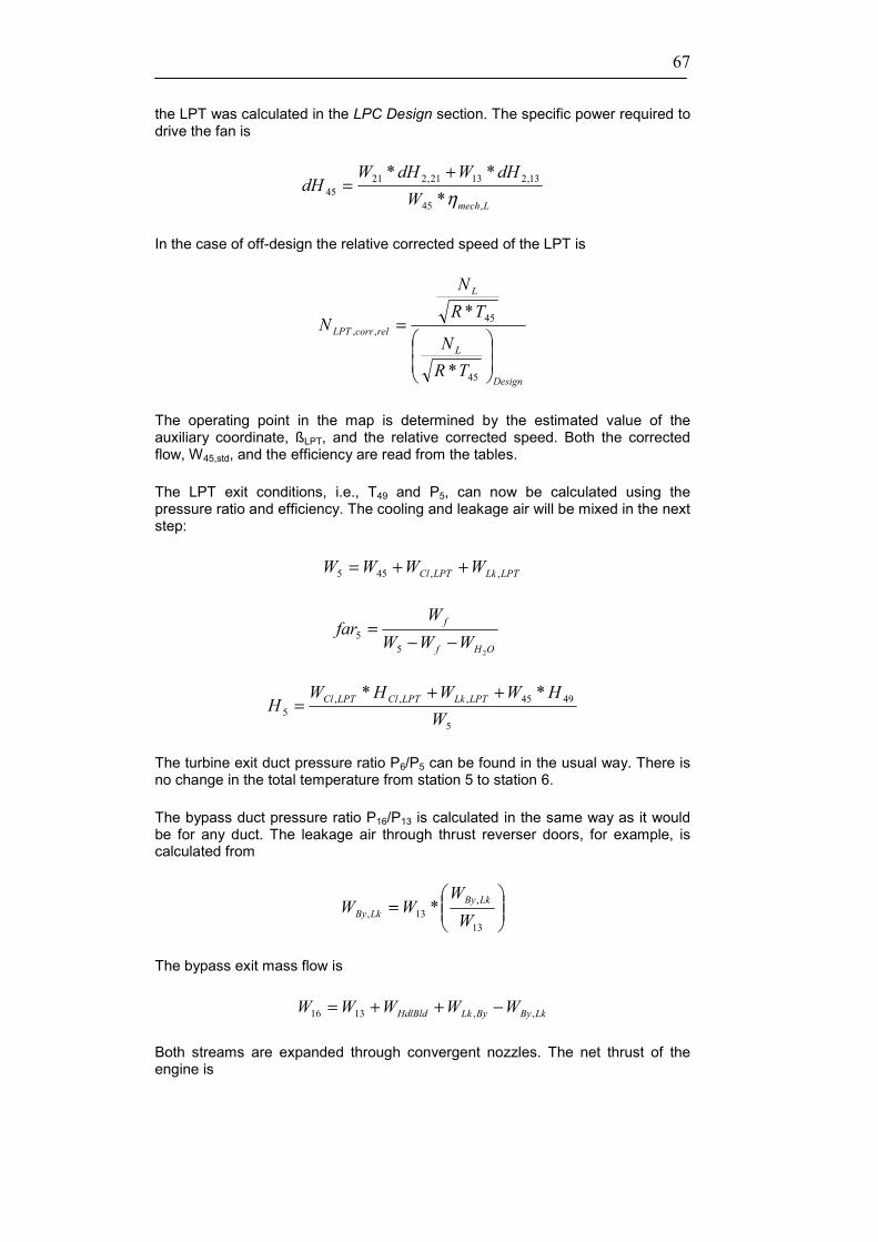
67
the LPT was calculated in the LPC Design section. The specific power required to drive the fan is
LmechWdHWdHW
dH,45
13,21321,22145 *
**η+
=
In the case of off-design the relative corrected speed of the LPT is
Design
L
L
relcorrLPT
TRN
TRN
N
=
45
45,,
*
*
The operating point in the map is determined by the estimated value of the auxiliary coordinate, ßLPT, and the relative corrected speed. Both the corrected flow, W45,std, and the efficiency are read from the tables.
The LPT exit conditions, i.e., T49 and P5, can now be calculated using the pressure ratio and efficiency. The cooling and leakage air will be mixed in the next step:
LPTLkLPTCl WWWW ,,455 ++=
OHf
f
WWWW
far25
5 −−=
5
4945,,,5
**W
HWWHWH LPTLkLPTClLPTCl ++
=
The turbine exit duct pressure ratio P6/P5 can be found in the usual way. There is no change in the total temperature from station 5 to station 6.
The bypass duct pressure ratio P16/P13 is calculated in the same way as it would be for any duct. The leakage air through thrust reverser doors, for example, is calculated from
=
13
,13, *
WW
WW LkByLkBy
The bypass exit mass flow is
LkByByLkHdlBld WWWWW ,,1316 −++=
Both streams are expanded through convergent nozzles. The net thrust of the engine is

68
02181818,1818
8,88,88
*)(***)(***
VWPPACVWPPACVWF
ambsFG
ambsFGN
−−++−+=
In addition to the real nozzle velocities the ideal velocities are also calculated. The ideal velocities imply a full expansion from stations 18 and 8 to ambient pressure. The ratio Vid,18/Vid,8 can be used to find the optimum combination of the fan outer pressure ratio and the bypass ratio.
Propulsion efficiency is calculated as follows:
0188
02
*)(*
1
2
VWWVWFN
prop
++
+=η
Core efficiency is given by
FHVWVdHW
f
iscore *
)2/(* 2045 −
=η
The enthalpy difference dHis is calculated assuming an isentropic expansion from the intermediate station 47 to ambient pressure. Station 47 is found by starting from station 45 and expanding the flow with the LPT efficiency to get the power needed for compressing the core flow W21 from P2 to P21.
For the turbofan cycle you can get both a temperature-entropy and an enthalpy-entropy diagram. Often the region around station 2 will be very crowded. You should then enlarge this part of the graph.

69
2.1.6. Two-spool mixed flow turbofan
The calculation starts with the intake. The altitude, flight Mach number and ∆TISA yield the ambient temperature and pressure, the flight velocity and the total engine inlet conditions T1 and P1. The pressure at the fan inlet can be easily calculated from the input value of the intake pressure ratio P2/P1 or from the value read from the intake map.
In the case of off-design the relative corrected fan spool speed is
Design
L
L
relcorrLPC
TRN
TRN
N
=
2
2,,
*
*
There are three ways to simulate the off-design behavior of the low-pressure compressor (LPC). The first option is the same as described for the unmixed turbofan engine in the previous chapter. This type of calculation is based on the map for the outer fan (bypass).
The outer fan map is read with help of the relative corrected speed and the auxiliary map coordinate ßLPC. This yields the standard day corrected mass flow W2√ΘR,2/δ2, the isentropic efficiency η2,13, the pressure ratio P13/P2 and the surge margin. NL and ßLPC are estimated values in an off-design calculation. W2 can easily be derived from W2√ΘR,2/δ2, T2 and P2. The values for the efficiency η2,21 and the pressure ratio P21/P2 of the inner stream are derived from those of the outer stream:
Design
=
13,2
21,213,221,2 *
ηη
ηη
DesignPPPP
PP
PP
−
−
−+=
1
1*11
2
13
2
21
2
13
2
21
The second method uses an independent map for the booster (core flow compressor). From the outer map we get the bypass flow flow W13√ΘR,2/δ2, and from the booster map we get W21√ΘR,2/δ2. Obviously the corrected speed is the same for the outer fan and the booster. However, two auxiliary coordinate values ßLPC and ßIPC are needed.
The third method uses also two maps, but they give both the same total mass flow W2√ΘR,2/δ2. This type of characteristic is called a Split Map and needs only one auxiliary coordinate ßLPC. The surge margin in a split map is calculated from
Fan map

70
the bypass flow conditions when the design bypass ratio is greater than 1. Otherwise, the core flow defines the surge margin.
In the case of design calculations, isentropic or polytropic efficiencies, and pressure ratios for both the core and the bypass stream are input quantities. The compression calculation yields the fan exit temperatures T21 and T13 as well as the specific works dH2,21 and dH2,13.
There are several input options for the mass flow in the case of design calculations. The first option uses W2√ΘR,2/δ2 as input. W2 can be derived easily. The mass flows of the individual streams are calculated from the bypass ratio:
BPRWW
+=
12
21
21213 WWW −=
The second option uses W25√ΘR,25/δ25 as the input of mass flow. Since T25 and P25 are known, W25 can be calculated. In the inter-duct between the compressors a handling bleed can be subtracted. W21 is then equal to W25+WHdlBld.
W13 is BPR*W21, and W2 is the sum of W21 and W13. Using W25√ΘR,25/δ25 as input is useful in cycle studies involving the same core engine. Turbine design calculations are easier to do with a fixed core size, since all diameters needed as input will stay the same.
The third input option for the engine mass flow is used in the case of the simulation of an engine with a given gas generator. For this purpose you need a map for the high-pressure compressor HPC. You can use a given map or you may scale a map as required for your specific task.
In the unscaled map you must enter the map speed value N/√Tmap and a value for the auxiliary coordinate ßHPC in such a way that the operating point in the map fits to the other data of your cycle design point.
Mass flow input options

71
When you want to use a scaled map then you have to enter in addition to the map speed value N/√Tmap and a value for the auxiliary coordinate ßHPC the true values for the corrected flow W25√ΘR,25/δ25, the pressure ratio P3/P25 and the efficiency ηHPC.
After the map scaling is completed one can modify the operating point in the HPC map by changing the values for the map speed N/√Tmap and the auxiliary coordinate ßHPC. Pressure ratio, corrected flow and efficiency will be read from the map. The flow capacities and pressure ratios of the turbines that are needed for the selected HPC operating point will be calculated.
To perform a simulation of inlet flow distortion as well as to study the transient behavior one needs some engine geometry data. They will be calculated if you select LPC Design. Then W2, T2, P2, the blade tip velocity, the inlet hub-tip radius ratio and the axial Mach number are used to calculate the tip diameter, the relative and circumferential Mach numbers, and the angular velocity.
For the description of the inlet flow distortion the static quantities in the aerodynamic interface plane are required. The flow area is derived from the fan tip diameter.
For the high-pressure compressor equivalent HPC design calculations can be selected. Note that you can only do turbine design calculations if the spool speed is known, i.e., the corresponding Compressor Design has been switched on.
In an operating line calculation and during the simulation of the transient behavior you can select the handling bleed to be switched automatically. The handling bleed is subtracted between stations 21 and 25 if independent fan maps for the core and the bypass stream are selected (B_Map=1). For the other fan map options the handling bleed is subtracted from the high-pressure compressor.
The bleed valve is closed when the relative corrected compressor speed is higher than NH,corr,rel,2. It will be fully open as long as the corrected speed is lower than NH,corr,rel,1. If the corrected spool speed is between these boundaries then the handling bleed flow is interpolated linearly:
−−
−
=
1,,,2,,,
1,,,,,
max2121 1**
relcorrHrelcorrH
relcorrHrelcorrHHdlBldHdlBld NN
NNWW
WW
Distortion and transient simulations
Aerodynamic interface plane
Automatic handling bleed

72
If independent fan maps for the core and the bypass stream are selected (B_Map=1), then the automatic bleed valve position is scheduled with the low-pressure spool speed NL,corr,rel.
The pressure at the inlet to the high-pressure compressor is derived from the inter-duct pressure ratio P25/P21 for design calculations, whereas it depends on the corrected flow for off design calculations. There is no change in total temperature and mass flow from station 21 to station 25.
In off-design the compressor map is read using estimated values for the auxiliary coordinate ßHPC and the relative corrected speed:
Design
H
H
relcorrHPC
TRN
TRN
N
=
25
25,,
*
*
The map reading provides W25√ΘR,25/δ25, the pressure ratio P3/P25, the efficiency and the surge margin. The compression calculation for the HPC yields T3, P3 and dH25,3.
132 21 25
3 4
64 8
63
44 45 5
16
6
31
163
a bc
HP leak to LPT exit
LPT cooling
leakage from bypassa HP leakage to bypassb NGV coolingc HPT cooling
handling bleed
overboard bleeds
41
GasTurbMFanHBPRPPT.WMF
Now we look at the internal air system. The high-pressure turbine (HPT) cooling air mass flow is
=
25
,25, *
WW
WW HPTClHPTCl
This amount of cooling air is assumed not to do any work; it is mixed with the main gas stream behind the high-pressure turbine. The nozzle guide vane (NGV) cooling air mass flow is calculated in a similar manner:
HPC map
Internal air system

73
=
25
,25, *
WW
WW NGVClNGVCl
The NGV cooling air is mixed with the main stream at station 41 upstream of the rotor(s), consequently this amount of air does work in the turbine. Leakages from the compressor exit to the bypass and to low-pressure turbine exit can also be taken into account:
=
25
,25, *
WW
WW BylkBylk
=
25
,25, *
WW
WW LPTlkLPTlk
The low-pressure turbine (LPT) needs also some cooling air
=
25
,25, *
WW
WW LPTClLPTCl
This air is often taken as an inter-stage bleed from the high-pressure compressor. Specific work done on this air is
3,25,, *dHfdH LPTClLPTCl =
The LPT cooling air is not assumed to do any work, neither in the HPT nor in the LPT. This air will be mixed with the main stream behind the LPT.
An overboard bleed mass flow can be specified as a linear combination of a relative and an absolute amount
2,25
1,25 * Bld
BldBld W
WW
WW +
=
The work done on the overboard bleed air is:
3,25*dHfdH BldBld =
For the compression of the NGV cooling air and the turbine rotor cooling air the specific power dH25,3 is required. The mass flow at the compressor exit, W3, is the flow without the inter-stage bleeds that are not fully compressed (an inter-stage bleed is characterized by 0<fBld<1):
BldLPTCl WWWW −−= ,253
Between stations 3 and 31 the fully compressed bleed flows are subtracted:
LPTlkBylkHPTClNGVClHdlBld WWWWWWW ,,,,331 −−−−−=

74
The pressure loss in the burner is calculated as usual: in design calculations the pressure ratio P4/P3 is given, whereas in off-design calculations it is a function of the corrected flow and the design point pressure ratio.
The amount of fuel is calculated from the required fuel-air-ratio, which in turn depends on burner pressure, inlet temperature, humidity of the incoming air and temperature rise.
)(*/23134 OHf WWfarW −= η
The burner exit flow is W4=W31+Wf and the turbine nozzle guide vane exit flow W41 equals W4+WCl,NGV. The fuel-air-ratio far41 is
OHf
f
WWWW
far241
41 −−=
Now it is possible to calculate the enthalpy corresponding to the Stator Outlet Temperature (SOT) or Rotor Inlet Temperature (RIT) of the turbine:
413,4441 /)**( WHWHWH NGVCl+=
The power delivered by the high-pressure turbine (HPT) is a product of W41 and the specific power dH41,44. The energy balance with all power requirements, including the customer power offtake PWX, is given by
Hmech
BldBldLPTClLPTClmainC
WPWXdHWdHWPW
dH,41
,,,44,41 *
**η
+++=
PWC,main is the power needed to compress the main gas stream:
3,25,,,,31, *)( dHWWWWWWPW LPTLkByLkHPTclNGVClHdlBldmainC +++++=
If Turbine Design is selected then the isentropic efficiency of the HPT is calculated, otherwise, it is given as an input property. In off-design simulations the efficiency is read from the HPT map.
The relative corrected high-pressure turbine speed is
Design
H
H
relcorrHPT
TRN
TRN
N
=
41
41,,
*
*
The turbine efficiency and the corrected flow are read from the map with the known relative corrected spool speed and the auxiliary coordinate ßHPT. The efficiency can be modified in off-design simulations by a tip clearance correction term, which is a function of the relative mechanical spool speed:
Burner
High pressure turbine

75
HHclearancetip N
Nδδηη *)1( −=∆
From the specific work dH41,44 and the efficiency we can calculate P43=P44 and the turbine rotor exit temperature T43. Then the turbine rotor cooling air is added: W45=W41+WCl,HPT. The LPT inlet enthalpy H45 is calculated using the energy balance:
45
,34141414345
**),,(W
WHWwarfarThH HPTCl+
=
The fuel air ratio comes from
OHf
f
WWWW
far245
45 −−=
Pressure losses in the inter-duct between both turbines can be calculated in several ways. For design calculations, when turbine efficiency is taken from input, P45/P44 is a given quantity. If Turbine Design is selected and a value for the reference Mach number M44>0 is given, then the pressure loss will be adjusted to the actual Mach number level. If the reference Mach number is not given, then the input value of P45/P44 is used again. During off-design the losses vary with the corrected flow in the same way as in any duct.
Usually, the low-pressure turbine (LPT) efficiency is an input value. Efficiency can also be derived from turbine design calculations, however. The rotational speed of the LPT was calculated in the LPC Design section. The specific power required to drive the fan is
LmechWdHWdHW
dH,45
13,21321,22145 *
**η+
=
In the case of off-design the relative corrected speed of the LPT is
Design
L
L
relcorrLPT
TRN
TRN
N
=
45
45,,
*
*
The operating point in the map is determined by the estimated value of the auxiliary coordinate, ßLPT, and the relative corrected speed. Both the corrected flow, W45,std, and the efficiency are read from the tables.
The LPT exit conditions, i.e., T49 and P5, can now be calculated using the pressure ratio and efficiency. The cooling and leakage air will be mixed in the next step:
LPTLkLPTCl WWWW ,,455 ++=
Turbine inter-duct

76
OHf
f
WWWW
far25
5 −−=
5
4945,,,5
**W
HWWHWH LPTLkLPTClLPTCl ++
=
The turbine exit duct pressure ratio P6/P5 can be found in the usual way. There is no change in the total temperature from station 5 to station 6.
The bypass duct pressure ratio P16/P13 is calculated in the same way as it would be for any duct. The leakage air through thrust reverser doors, for example, is calculated from
=
13
,13, *
WW
WW LkByLkBy
The bypass exit mass flow is
LkByByLkHdlBld WWWWW ,,1316 −++=
132521 3 4 4445
52
6
16
63
647 8 9163
a HP leakage to bypassb NGV coolingc HPT coolingd Handling bleed
HP leak to LPT exit
bc
LPT cooling
overboard bleeds
leakage from bypass
d a
4131
GasTurbMFanRHCDPPT.WMF
The inlet conditions for the cold side of the mixer are those from station 16. However, a nozzle cooling mass flow may be subtracted from the bypass exit mass flow first for engines with an afterburner:
−=
16
,1616163 *
WW
WWW NozCl
Mixer and afterburner

77
Now both the core and the bypass stream will be mixed. The hot stream mixer pressure ratio P63/P6 is assumed to vary with corrected flow in off-design simulations. The area A63 is derived from the prescribed Mach number M63 in the case of design. The cold stream mixer pressure ratio P163/P16 is dependent from corrected flow in off-design, too. The cold mixer inlet area A163 is derived from the given Mach number M163 during design calculations.
The mixer area A64 is equal to the sum of A63 and A163. It can be specified by input or calculated from the mean mixer Mach number M64 during design calculations. In off-design the static pressure balance between Ps,63 and Ps,163 is retained. The areas A63 and A163 are taken from the design point calculation. In off-design simulations you can apply modifiers to the design point mixer areas. Note that in this case the total area A64 is recalculated as the sum of A63 and A163.
In the mixing calculation the program uses the conservation of energy for finding T64. The mass flow W64 is the sum of W6 and W161. P64 is calculated on the basis of conservation of momentum in a constant area duct.
Then the fuel-air-ratio far7 is calculated from the specified reheat exit temperature T7. Reheat fuel flow is then
−= 1*
64
7, far
farWW fRHf
The total reheat exit mass flow amounts to W7=W64+Wf,RH. The fundamental pressure loss caused by the heat addition will then be calculated. The correlations of the Rayleigh line, i.e., heat addition in a pipe with constant area, are used. The inlet Mach number for this calculation is M64.
Before the nozzle calculation starts, nozzle cooling air is mixed with the main stream. The nozzle total temperature will therefore be lower than T7, if nozzle cooling air is considered.
Two types of nozzles can be calculated: a convergent nozzle and a convergent-divergent nozzle with a prescribed nozzle area ratio A9/A8. The fully mixed net thrust for a convergent nozzle is
028,888, *)(*** VWPPACVWF ambsFGidN −−+=
For the convergent-divergent nozzle it is
029,998, *)(*** VWPPACVWF ambsFGidN −−+=
The pressure term A9*(Ps,9-Pamb) will be negative if the nozzle area ratio is too big for the pressure ratio.
These formulae apply to a fully mixed flow. However, in reality full mixing is not achieved. The thrust for a partially mixed flow is calculated on the basis of the separate expansion of W16 and W6 to ambient conditions. For a convergent nozzle the cold and hot stream gross thrusts are
)(*** ,16, ambcscFGccg PPACVWF −+= )(*** ,6, ambhshFGhhg PPACVWF −+=
Nozzle

78
The areas Ac and Ah are calculated from continuity. The cold and hot stream thrust for a convergent-divergent nozzle is found in a similar matter. The partially mixed thrust is then calculated:
02,,, *)(*)1(* VWFFFF hgcgmixidgmixN −+−+= ηη
Note that in the case of reheat the mixing efficiency ηmix is set to 1.0 internally as combustion is assumed to enhance the mixing process.
Propulsion efficiency is
08
02Pr
**
1
2
VWVWFN
op ++
=η
Core efficiency is given by:
FHVWVdHW
f
iscore *
)2/(* 2048 −=η
The enthalpy difference dHis is calculated assuming an isentropic expansion from the intermediate station 47 to ambient pressure. Station 47 is found by starting from station 45 and expanding the flow with the LPT efficiency to get the power needed for compressing the core flow W21 from P2 to P21.
For the mixed flow turbofan cycle you can get both a temperature-entropy and an enthalpy-entropy diagram. Often the region around station 2 will be very crowded. You should then enlarge this part of the graph.

79
2.1.7. Geared turbofan
The calculation starts with the intake. The altitude, flight Mach number and ∆TISA yield the ambient temperature and pressure, the flight velocity and the total engine inlet conditions T1 and P1. The pressure at the compressor inlet can be easily calculated from the input value of the intake pressure ratio P2/P1 or from the value read from the intake map.
In the case of design calculations the total corrected engine mass flow W2√ΘR,2/δ2 is an input. W2 can be derived easily. The mass flows of the individual streams are calculated from the bypass ratio:
BPRWW
+=
12
21
21213 WWW −=
Further input for design calculations are the isentropic or polytropic efficiencies and the pressure ratios for both streams.
In the case of off-design the relative corrected fan speed is
Design
L
L
relcorrL
TRN
TRN
N
=
2
2,,
*
*
Then the fan map - which primarily is valid for the outer fan (bypass) stream - is read with the help of the relative corrected speed and the auxiliary map coordinate ßLPC. This yields the standard day corrected mass flow W2√ΘR,2/δ2, the isentropic efficiency η2,13, the pressure ratio P13/P2 and the surge margin. NL and ßLPC are estimated values in an off-design calculation. W2 can easily be derived from W2√ΘR,2/δ2, T2 and P2. The efficiency η2,21 and the pressure ratio P21/P2 for the inner stream are derived from those of the outer stream:
Design
=
13,2
21,213,221,2 *
ηη
ηη
DesignPPPP
PP
PP
−
−
−+=
1
1*11
2
13
2
21
2
13
2
21
Fan Map

80
The compression is calculated as usual. It yields the fan exit temperatures T21 and T13 as well as the specific works dH2,21 and dH2,13.
To perform a simulation of inlet flow distortion as well as to study the transient behavior one needs some engine geometry data. They will be calculated if you select LPC Design. Then W2, T2, P2, the blade tip velocity, the inlet hub-tip radius ratio and the axial Mach number are used to calculate the tip diameter, the relative and circumferential Mach numbers, and the angular velocity.
For the description of the inlet flow distortion the static quantities in the aerodynamic interface plane are required. The flow area is derived from the fan tip diameter.
Next is the calculation of the intermediate-pressure compressor (IPC) or booster. In the case of design calculations the pressure ratio and the efficiency are input values.
In off-design the IPC map is read with estimated values for the auxiliary coordinate ßIPC and the relative corrected speed of the intermediate spool:
Design
I
I
relcorrI
TRN
TRN
N
=
21
21,,
*
*
Note that the rotational speed of the booster differs from NL by the gear ratio. The exit station of the IPC is station 24. The corrected flow W21√ΘR,21/δ21, the pressure ratio P24/P21 and efficiency η21,24 are read from the map. The compression calculation yields T24, P24 and dH21,24.
There are several input options for the mass flow in the case of design calculations. The first option uses W2√ΘR,2/δ2 as input. W2 can be derived easily. The mass flows of the individual streams are calculated from the bypass ratio:
BPRWW
+=
12
21
21213 WWW −=
The second option uses W25√ΘR,25/δ25 as the input of mass flow. Since T25 and P25 are known, W25 can be calculated. In the inter-duct between the compressors a handling bleed can be subtracted. W21 is then equal to W25+WHdlBld.
W13 is BPR*W21, and W2 is the sum of W21 and W13. Using W25√ΘR,25/δ25 as input is useful in cycle studies involving the same core engine. Turbine design calculations are easier to do with a fixed core size, since all diameters needed as input will stay the same.
The third input option for the engine mass flow is used in the case of the simulation of an engine with a given gas generator. For this purpose you need a map for the high-pressure compressor HPC. You can use a given map or you may scale a map as required for your specific task.
Distortion and transient simulations
Aerodynamic interface plane
Intermediate Compressor
Mass flow input options

81
In the unscaled map you must enter the map speed value N/√Tmap and a value for the auxiliary coordinate ßHPC in such a way that the operating point in the map fits to the other data of your cycle design point.
After the map scaling is completed one can modify the operating point in the HPC map by changing the values for the map speed N/√Tmap and the auxiliary coordinate ßHPC. Pressure ratio, corrected flow and efficiency will be read from the map. The flow capacities and pressure ratios of the turbines that are needed for the selected HPC operating point will be calculated.
For the high-pressure compressor equivalent HPC design calculations can be selected. Note that you can only do turbine design calculations if the spool speed is known, i.e., the corresponding Compressor Design has been switched on.
The pressure at the inlet to the high-pressure compressor (HPC) is derived from the inter-duct pressure ratio P25/P24 for design calculations, whereas it depends on the corrected flow for off design calculations. There is no change in total temperature from station 24 to station 25.
In an operating line calculation and during the simulation of the transient behavior you can select the handling bleed to be switched automatically. This bleed is closed when the relative corrected low-pressure compressor (LPC) speed is higher than NL,corr,rel,2. It will be open when the corrected speed is lower than
Handling Bleed
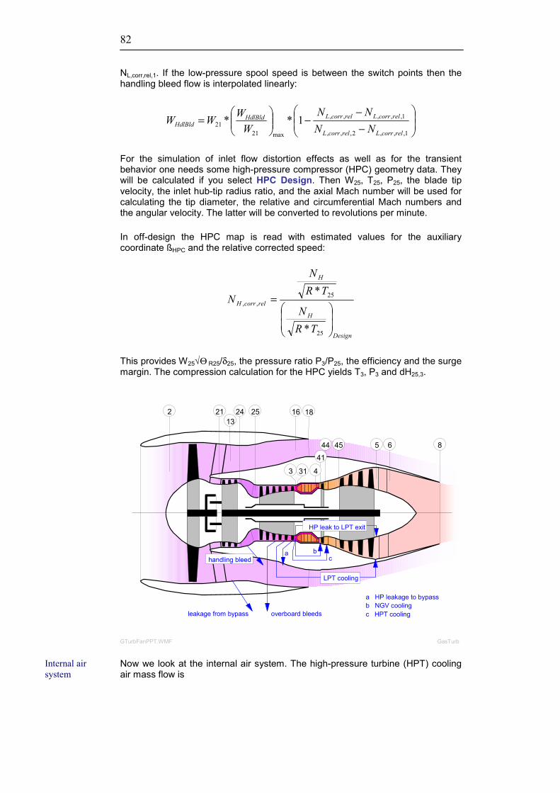
82
NL,corr,rel,1. If the low-pressure spool speed is between the switch points then the handling bleed flow is interpolated linearly:
−−
−
=
1,,,2,,,
1,,,,,
max2121 1**
relcorrLrelcorrL
relcorrLrelcorrLHdlBldHdlBld NN
NNWWWW
For the simulation of inlet flow distortion effects as well as for the transient behavior one needs some high-pressure compressor (HPC) geometry data. They will be calculated if you select HPC Design. Then W25, T25, P25, the blade tip velocity, the inlet hub-tip radius ratio, and the axial Mach number will be used for calculating the tip diameter, the relative and circumferential Mach numbers and the angular velocity. The latter will be converted to revolutions per minute.
In off-design the HPC map is read with estimated values for the auxiliary coordinate ßHPC and the relative corrected speed:
Design
H
H
relcorrH
TRN
TRN
N
=
25
25,,
*
*
This provides W25√Θ R25/δ25, the pressure ratio P3/P25, the efficiency and the surge margin. The compression calculation for the HPC yields T3, P3 and dH25,3.
13182 25
3
4144 45 5 6 8
1621 24
31 4
handling bleed
HP leak to LPT exit
LPT cooling
a bc
overboard bleeds
a HP leakage to bypassb NGV coolingc HPT coolingleakage from bypass
GasTurbGTurbFanPPT.WMF
Now we look at the internal air system. The high-pressure turbine (HPT) cooling air mass flow is
Internal air system

83
=
25
,25, *
WW
WW HPTClHPTCl
This amount of cooling air is assumed not to do any work; it is mixed with the main gas stream behind the high-pressure turbine. The nozzle guide vane (NGV) cooling air mass flow is calculated in a similar manner:
=
25
,25, *
WW
WW NGVClNGVCl
The NGV cooling air is mixed with the main stream at station 41 upstream of the rotor(s), consequently this amount of air does work in the turbine. Leakages from the compressor exit to the bypass and to low-pressure turbine exit can also be taken into account:
=
25
,25, *
WW
WW BylkBylk
=
25
,25, *
WW
WW LPTlkLPTlk
The low-pressure turbine (LPT) needs also some cooling air
=
25
,25, *
WW
WW LPTClLPTCl
This air is often taken as an inter-stage bleed from the high-pressure compressor. Specific work done on this air is
3,25,, *dHfdH LPTClLPTCl =
The NGV and HPT cooling air as well as the leaking air are compressed fully; the specific power required for this is dH25,3.
The LPT cooling air is assumed not to do any work, neither in the HPT nor in the LPT. This air will be mixed with the main stream behind the LPT.
An overboard bleed mass flow can be specified as a linear combination of a relative and an absolute amount
2,25
1,25 * Bld
BldBld W
WW
WW +
=
The work done on the overboard bleed air is:
3,25*dHfdH BldBld =

84
For the compression of the NGV cooling air and the turbine rotor cooling air the specific power dH25,3 is required. The mass flow at the compressor exit, W3, is the flow without the inter-stage bleeds that are not fully compressed (an inter-stage bleed is characterized by fBld<1):
BldLPTCl WWWW −−= ,253
Between stations 3 and 31 the fully compressed bleed flows are subtracted:
LPTlkBylkHPTClNGVCl WWWWWW ,,,,331 −−−−=
The pressure loss in the burner is calculated as usual: in design calculations the pressure ratio P4/P3 is given, whereas in off-design calculations it is a function of the corrected flow and the design point pressure ratio.
The amount of fuel is calculated from the required fuel-air-ratio, which in turn depends on burner pressure, inlet temperature, humidity of the incoming air and temperature rise.
)(*/23134 OHf WWfarW −= η
The burner exit flow is W4=W31+Wf and the turbine nozzle guide vane exit flow W41 equals W4+WCl,NGV. The fuel-air-ratio far41 is
OHf
f
WWWW
far241
41 −−=
Now it is possible to calculate the enthalpy corresponding to the Stator Outlet Temperature (SOT) or Rotor Inlet Temperature (RIT) of the turbine:
413,4441 /)**( WHWHWH NGVCl+=
The power delivered by the high-pressure turbine (HPT) is a product of W41 and the specific power dH41,44. The energy balance with all power requirements, including the customer power offtake PWX, is given by
Hmech
BldBldLPTClLPTClmainC
WPWXdHWdHWPW
dH,41
,,,44,41 *
**η
+++=
PWC,main is the power needed to compress the main gas stream:
3,25,,,,31, *)( dHWWWWWPW LPTLkByLkHPTclNGVClmainC ++++=
If Turbine Design is selected then the isentropic efficiency of the HPT is calculated, otherwise, it is given as an input property. In off-design simulations the efficiency is read from the HPT map.
The relative corrected high-pressure turbine speed is
Burner
High pressure turbine

85
Design
H
H
relcorrHPT
TRN
TRN
N
=
41
41,,
*
*
The turbine efficiency and the corrected flow are read from the map with the known relative corrected spool speed and the auxiliary coordinate ßHPT. The efficiency can be modified in off-design simulations by a tip clearance correction term, which is a function of the relative mechanical spool speed:
HHclearancetip N
Nδδηη *)1( −=∆
From the specific work dH41,44 and the efficiency we can calculate P43=P44 and the turbine rotor exit temperature T43. Then the turbine rotor cooling air is added: W45=W41+WCl,HPT. The LPT inlet enthalpy H45 is calculated using the energy balance:
45
,34141414345
**),,(W
WHWwarfarThH HPTCl+
=
The fuel air ratio comes from
OHf
f
WWWW
far245
45 −−=
Pressure losses in the inter-duct between both turbines can be calculated in several ways. For design calculations, when turbine efficiency is taken from input, P45/P44 is a given quantity. If Turbine Design is selected and a value for the reference Mach number M44>0 is given, then the pressure loss will be adjusted to the actual Mach number level. When the reference Mach number is not given, then the input value of P45/P44 is used again. During off-design the losses vary with the corrected flow in the same way as in any duct.
Usually, the low-pressure turbine (LPT) efficiency is an input value. Efficiency can also be derived from turbine design calculations, however. The rotational speed of the LPT was calculated in the LPC Design section. The specific power required to drive the fan is
45
24,2121,13,21321,22145
*/)**(W
dHWdHWdHWdH Lmech ++
=η
In the case of off-design the relative corrected speed of the LPT is
Turbine inter-duct

86
Design
L
L
relcorrLPT
TRN
TRN
N
=
45
45,,
*
*
The operating point in the map is determined by the estimated value of the auxiliary coordinate, ßLPT, and the relative corrected speed. Both the corrected flow, W45,std, and the efficiency are read from the tables.
The LPT exit conditions, i.e., T49 and P5, can now be calculated using the pressure ratio and efficiency. The cooling and leakage air will be mixed in the next step:
LPTLkLPTCl WWWW ,,455 ++=
OHf
f
WWWW
far25
5 −−=
5
4945,,,5
**W
HWWHWH LPTLkLPTClLPTCl ++
=
The turbine exit duct pressure ratio P6/P5 can be found in the usual way. There is no change in the total temperature from station 5 to station 6.
The bypass duct pressure ratio P16/P13 is calculated in the same way, as it would be for any duct. The leakage air through thrust reverser doors, for example, is calculated from
=
13
,13, *
WW
WW LkByLkBy
The bypass exit mass flow is
LkByByLkHdlBld WWWWW ,,1316 −++=
Both streams are expanded through convergent nozzles. The net thrust of the engine is
02181818,1818
8,88,88
*)(***)(***
VWPPACVWPPACVWF
ambsFG
ambsFGN
−−++−+=
In addition to the real nozzle velocities the ideal velocities are also calculated. The ideal velocities imply a full expansion from stations 18 and 8 to ambient pressure. The ratio Vid,18/Vid,8 is used to find the optimum combination of the fan outer pressure ratio and the bypass ratio.
Propulsion efficiency is calculated as follows:

87
0188
02
*)(*
1
2
VWWVWFN
prop
++
+=η
Core efficiency is given by
FHVWVdHW
f
iscore *
)2/(* 2045 −
=η
The enthalpy difference dHis is calculated assuming an isentropic expansion from the intermediate station 47 to ambient pressure. Station 47 is found by starting from station 45 and expanding the flow with the LPT efficiency to get the power needed for compressing the core flow W21 from P2 to P24.
Also for the turbofan cycle you can get both a temperature-entropy and an enthalpy-entropy diagram. Often the region around station 2 will be very crowded. You should then enlarge this part of the graph.

88

89
2.1.8. Three-spool mixed flow turbofan
The calculation starts with the intake. The altitude, flight Mach number and ∆TISA yield the ambient temperature and pressure, the flight velocity and the total engine inlet conditions T1 and P1. The pressure at the compressor inlet can be easily calculated from the input value of the intake pressure ratio P2/P1 or from the value read from the intake map.
In the case of design calculations the total corrected engine mass flow W2√ΘR,2/δ2 is an input. W2 can be derived easily. The mass flows of the individual streams are calculated from the bypass ratio:
BPRWW
+=
12
21
21213 WWW −=
Further input for design calculations are the isentropic or polytropic efficiencies and the pressure ratios for both streams.
In the case of off-design the relative corrected fan speed is
Design
L
L
relcorrL
TRN
TRN
N
=
2
2,,
*
*
Then the fan map - which primarily is valid for the outer fan (bypass) stream - is read with the help of the relative corrected speed and the auxiliary map coordinate ßLPC. This yields the standard day corrected mass flow W2√ΘR,2/δ2, the isentropic efficiency η2,13, the pressure ratio P13/P2 and the surge margin. NL and ßLPC are estimated values in an off-design calculation. W2 can easily be derived from W2√ΘR,2/δ2, T2 and P2. The efficiency η2,21 and the pressure ratio P21/P2 for the inner stream are derived from those of the outer stream:
Design
=
13,2
21,213,221,2 *
ηη
ηη
DesignPPPP
PP
PP
−
−
−+=
1
1*11
2
13
2
21
2
13
2
21
Fan Map

90
The compression is calculated as usual. It yields the fan exit temperatures T21 and T13 as well as the specific works dH2,21 and dH2,13.
To perform a simulation of inlet flow distortion as well as to study the transient behavior one needs some engine geometry data. They will be calculated if you select LPC Design. Then W2, T2, P2, the blade tip velocity, the inlet radius ratio and the axial Mach number are used to calculate the tip diameter, the relative and circumferential Mach numbers, and the angular velocity. To obtain a description of the inlet flow distortion the static quantities in the aerodynamic interface plane are required. The flow area is calculated from the fan tip diameter.
Next is the calculation of the intermediate-pressure compressor (IPC) or booster. In the case of design calculations the pressure ratio and the efficiency are input values.
In off-design the IPC map is read with estimated values for the auxiliary coordinate ßIPC and the relative corrected speed of the intermediate spool:
Design
I
I
relcorrI
TRN
TRN
N
=
21
21,,
*
*
The exit station of the IPC is station 24. The corrected flow W21√ΘR,21/δ21, the pressure ratio P24/P21 and efficiency η21,24 are read from the map. The compression calculation yields T24, P24 and dH21,24.
3 521 3124
48
25
2
64
6
16
414
43
4547
13
163
637
98
handling bleed
overboard bleeds
leakage from bypass
NGVCool.
IPT NGV cooling
HPT cooling
HP leak to LPT exit
IPT cooling
LPT cooling
leakage to bypass
GasTurbM3spRHCDPPT.WMF
For the simulation of inlet flow distortion effects as well as for the transient behavior one needs some IPC geometry data. They will be calculated if you select IPC Design. Then W21, T21, P21, the blade tip velocity, the inlet radius ratio, and the axial Mach number will serve as a basis for calculating the tip diameter,
Intermediate Compressor

91
the relative and circumferential Mach numbers as well as the angular velocity. The latter will be converted to revolutions per minute.
The pressure at the inlet to the high-pressure compressor (HPC) is derived from the inter-duct pressure ratio P25/P24 for design calculations, whereas it depends on the corrected flow for off design calculations. There is no change in total temperature from station 24 to station 25.
In an operating line calculation and during the simulation of the transient behavior you can select the handling bleed to be switched automatically. This bleed valve is closed if the relative corrected low-pressure compressor (LPC) speed is higher than NL,corr,rel,2. It will be open if the corrected speed is lower than NL,corr,rel,1. If the low-pressure spool speed is between these boundaries then the handling bleed flow is interpolated linearly:
−−
−
=
1,,,2,,,
1,,,,,
max2121 1**
relcorrLrelcorrL
relcorrLrelcorrLHdlBldHdlBld NN
NNWWWW
For the simulation of inlet flow distortion effects as well as for the transient behavior one needs some high-pressure compressor (HPC) geometry data. They will be calculated if you select HPC Design in a similar way as the IPC geometry data.
In off-design the HPC map is read with estimated values for the auxiliary coordinate ßHPC and the relative corrected speed:
Design
H
H
relcorrH
TRN
TRN
N
=
25
25,,
*
*
This provides W25√ΘR25/δ25, the pressure ratio P3/P25, the efficiency and the surge margin. The compression calculation for the HPC yields T3, P3 and dH25,3.
Now we look at the internal air system. The high-pressure turbine (HPT) cooling air mass flow is
=
25
,25, *
WW
WW HPTClHPTCl
This amount of cooling air is assumed not to do any work; it is mixed with the main gas stream behind the HP turbine. The nozzle guide vane cooling air mass flow is calculated in a similar manner:
=
25
,25, *
WW
WW NGVClNGVCl
The NGV cooling air is mixed with the main stream at station 41 upstream of the rotor(s), consequently this amount of air does work in the turbine.
Handling Bleed
Internal Air System

92
The overboard bleed mass flow can be entered as a linear combination of a relative and an absolute amount
2,25
1,25 * Bld
BldBld W
WW
WW +
=
The work done on the overboard bleed air is:
3,25*dHfdH BldBld =
Furthermore, there can be leakage from the high-pressure region to the bypass and to the region downstream of the LPT:
=
25
,25, *
WW
WW ByLkByLk
=
25
,25, *
WW
WW LPTLkLPTLk
The NGV and HPT cooling air as well as the leaking air are compressed fully; the specific power required for this is dH25,3. The intermediate-pressure turbine (IPT) also requires also some cooling air both on the guide vane and the rotor:
=
25
,,25,, *
WW
WW IPTNGVClIPTNGVCl
=
25
,25, *
WW
WW IPTClIPTCl
This cooling air is usually taken from an inter-stage bleed of the high-pressure compressor. The work done on this air is
3,25,, *dHfdH IPTClIPTCl =
The IPT cooling air is assumed not to do any work, neither in the HPT nor in the IPT. The air will be mixed with the core stream behind the IPT. The cooling air temperature for the IPT is derived from the enthalpy:
)( ,25, IPTClIPTCl dHHfT +=
For the cooling of the low-pressure turbine also inter-stage bleed air may be used:
=
25
,25, *
WW
WW LPTClLPTCl
3,25,, *dHfdH LPTClLPTCl =
The LPT cooling air is assumed not to do any work neither in the HPT, the IPT nor in the LPT. The air will be mixed with the core stream behind the LPT. The cooling air temperature for the LPT is derived from the enthalpy:

93
)( ,25, LPTClLPTCl dHHfT +=
The mass flow at the compressor exit W3 is the flow with the inter-stage bleeds subtracted:
BldLPTClIPTClIPTNGVCl WWWWWW −−−−= ,,,,253
Between stations 3 and 31 the fully compressed bleeds are subtracted. Burner inlet flow is:
ByLkLPTLkHPTClNGVCl WWWWWW ,,,,331 −−−−=
In design calculations the burner pressure ratio P4/P3 is given, whereas in off-design calculations it is derived from the corrected flow and the design point pressure ratio. The amount of fuel is calculated from the required fuel-air-ratio, which in turn depends on burner pressure, inlet temperature, humidity and temperature rise.
)(*/23134 OHf WWfarW −= η
The burner exit flow is W4=W31+Wf, and the turbine nozzle guide vane exit flow is W41=W4+WCl,NGV. The fuel-air-ratio far41 is
OHf
f
WWWW
far241
41 −−=
Now it is possible to calculate the enthalpy corresponding to the HP turbine Stator Outlet Temperature (SOT) or Rotor Inlet Temperature (RIT):
413,4441 /)**( WHWHWH NGVCl+=
The power delivered by the high-pressure turbine (HPT) is a product of W41 and the specific power dH41,42. For the compression of the mainstream is needed
3,25,,,,31, *)( dHWWWWWPW LPTLkByLkHPTClNGVClmainC ++++=
The power required to compress the cooling air for the IPT is
IPTClIPTClIPTNGVClIPTC dHWWPW ,,,,, *)( +=
For the compression of the LPT cooling air is needed:
LPTClLPTClLPTC dHWPW ,,, *=
The energy balance with all power requirements for the high-pressure turbine amounts to
Hmech
BldBldLPTClIPTClmainC
WPWXdHWPWPWPW
dH,41
,,,42,41 *
*η
++++=
Burner

94
If Turbine Design is selected then the isentropic efficiency of the HPT is calculated, otherwise, it is given as an input property. In off-design simulations the efficiency is read from the HPT map.
The relative corrected high-pressure turbine speed is
Design
H
H
relcorrHPT
TRN
TRN
N
=
41
41,,
*
*
The turbine efficiency and the corrected flow are read from the map with the known relative corrected spool speed and the auxiliary coordinate ßHPT. The efficiency can be modified in off-design simulations by a tip clearance correction term, which is a function of the relative mechanical spool speed:
HHclearancetip N
Nδδηη *)1( −=∆
This allows calculating P42 = P43 and the HP turbine exit temperature T42.
Now the mass flow of the cooling air is taken into account: W43=W41+WCl,HPT. The IPT inlet enthalpy H43 is calculated on the basis of the energy balance:
43
,34141414243
**),,(W
WHWwarfarThH HPTCl+
=
The turbine exit fuel-air-ratio is
OHf
f
WWWW
far243
43 −−=
Pressure losses in the inter-duct between the high and the intermediate-pressure turbine can be calculated in several ways. For design calculations, when turbine efficiency is taken from input, P44/P43 is used as given. If HP turbine design is selected and a value for the reference Mach number M43>0 is given the pressure loss will be adjusted to the actual Mach number level. If the reference Mach number is not given, the input value of P44/P43 will be used again. In the case of off-design the losses vary with the corrected flow in the same way as in any duct.
The IPT nozzle guide vane exit flow is W45=W44+WCl,NGV,IPT. The fuel-air-ratio far45 is
OHf
f
WWWW
far245
45 −−=
The enthalpy corresponding with the IPT stator outlet temperature T45 can now be evaluated:
Inter-duct 1

95
45,,,444445 /)**( WHWHWH IPTClIPTNGVCl+=
Usually, the intermediate-pressure turbine (IPT) efficiency is an input value in cycle design calculations. The efficiency can also be derived from turbine design calculations, however. The rotational speed of the IPT is the same as that of the IPC (booster). During off-design calculations the efficiency is read from the IPT map.
The specific power required to drive the booster is
45,
24,212146,45 *
*W
dHWdH
Imechη=
Now the mass flow of the cooling air is taken into account: W47=W46+WCl,IPT. The LPT inlet enthalpy H47 =H48 is calculated on the basis of the energy balance:
47
,,4545454647
**),,(W
WHWwarfarThH IPTClIPTCl+
=
Pressure losses in the inter-duct between the intermediate- and the low-pressure turbine can be calculated in several ways. For design calculations, when the IPT efficiency is taken from input, P48/P47 is used as given. If IP turbine design is selected and a value for the reference Mach number M47>0 is given the pressure loss will be adjusted to the actual Mach number level. If the reference Mach number is not given, the input value of P48/P47 will be used again.
Usually, the low-pressure turbine (LPT) efficiency is an input value. The efficiency can also be derived from turbine design calculations, however. The rotational speed of the LPT is the same as that of the LPC (fan). During off-design calculations the efficiency is read from the LPT map.
The specific power required to drive the fan is
( )48,
13,21321,2215,48 *
**W
dHWdHWdH
Lmechη+
=
LPT exit conditions, i.e., T49 and P5, can now be calculated from the pressure ratio and the efficiency. Cooling and leakage air are added in the next step:
LPTLkLPTCl WWWW ,,475 ++=
OHf
f
WWWW
far25
5 −−=
5
49473,,,5
***W
HWHWHWH LPTLkLPTClLPTCl ++
=
The turbine exit duct pressure ratio P6/P5 is calculated in the usual way.
The bypass duct pressure ratio P16/P13 is calculated in the same way as it is for any duct. The bypass leakage air is calculated from
Inter-duct 2

96
=
13
,13, *
WW
WW LkByLkBy
The inlet conditions for the cold side of the mixer are those from station 16. However, a nozzle cooling mass flow may first be subtracted from the bypass exit mass flow for engines with an afterburner:
−=
16
,1616163 *
WW
WWW NozCl
Now both the core and the bypass stream will be mixed. The hot stream mixer pressure ratio P63/P6 is assumed to vary with corrected flow in off-design simulations. The cold stream mixer pressure ratio P163/P16 is dependent on corrected flow in off-design, too. The mixer area A64 is equal to the sum of A63 and A163. A64 can be specified by input or is calculated from the mean mixer Mach number M64 during design calculations. In off-design the static pressure balance between Ps,63 and Ps,163 is retained. The areas A63 and A163 are taken from the design point calculation.
In off-design simulations you can apply modifiers to the design point mixer areas. Note that in this case the total area A64 is recalculated as the sum of A63 and A163.
In the mixing calculation the program uses the conservation of energy for finding T64. The mass flow W64 is the sum of W6 and W161. P64 is calculated on the basis of conservation of momentum in a constant area duct.
Then the fuel-air-ratio far7 is calculated from the specified reheat exit temperature T7. Reheat fuel flow is then
−= 1*
64
7, far
farWW fRHf
The total reheat exit mass flow amounts to W7=W64+Wf,RH. The fundamental pressure loss caused by the heat addition will then be calculated. The correlations of the Rayleigh line, i.e., heat addition in a pipe with constant area, are used. The inlet Mach number for this calculation is M64.
Before the nozzle calculation starts, nozzle cooling air is mixed with the main stream. The nozzle total temperature will therefore be lower than T7, if nozzle cooling air is considered.
Two types of nozzles can be calculated: a convergent nozzle and a convergent-divergent nozzle with a prescribed nozzle area ratio A9/A8. The fully mixed net thrust for a convergent nozzle is
028,888, *)(*** VWPPACVWF ambsFGidN −−+=
For the convergent-divergent nozzle it is
029,998, *)(*** VWPPACVWF ambsFGidN −−+=
Mixer and afterburner
Nozzle
97
The pressure term A9*(Ps,9-Pamb) will be negative if the nozzle area ratio is too big for the pressure ratio.
These formulas apply to a fully mixed flow. However, in reality full mixing is not achieved. The thrust for a partially mixed flow is calculated on the basis of the separate expansion of W16 and W6 to ambient conditions. For a convergent nozzle the cold respectively hot stream gross thrust is
)(*** ,16, ambcscFGccg PPACVWF −+= )(*** ,6, ambhscFGhhg PPACVWF −+=
The areas Ac and Ah are calculated from continuity. The cold and hot stream thrust for a convergent-divergent nozzle is found in a similar matter. The partially mixed thrust is then calculated:
02,,, *)(*)1(* VWFFFF hgcgmixidgmixN −+−+= ηη
Note that in the case of reheat the mixing efficiency ηmix is set to 1.0 internally as combustion is assumed to enhance the mixing process.
Propulsion efficiency is
08
02Pr
**
1
2
VWVWFN
op ++
=η
Core efficiency is given by:
FHVWVdHW
f
iscore *
)2/(* 2048 −=η
The enthalpy difference dHis is calculated assuming an isentropic expansion from the intermediate station 485 to ambient pressure. Station 485 is found by starting from station 48 and expanding the flow with the LPT efficiency to get the power needed for compressing the core flow W21 from P2 to P21.
For the mixed flow turbofan cycle you can get both a temperature-entropy and an enthalpy-entropy diagram. Often the region around station 2 will be very crowded. You should then enlarge this part of the graph.

98

99
2.1.9. Intercooled recuperated turbofan
The calculation starts with the intake. The altitude, flight Mach number and ∆TISA yield the ambient temperature and pressure, the flight velocity and the total engine inlet conditions T1 and P1. The pressure at the compressor inlet can be easily calculated from the input value of the intake pressure ratio P2/P1 or from the value read from the intake map.
In the case of design calculations the total corrected engine mass flow W2√ΘR,2/δ2 is an input. W2 can be derived easily. The mass flows of the individual streams are calculated from the bypass ratio:
BPRWW
+=
12
21
21213 WWW −=
Further input for design calculations are the isentropic or polytropic efficiencies and the pressure ratios for both streams.
In the case of off-design the relative corrected fan speed is
Design
L
L
relcorrL
TRN
TRN
N
=
2
2,,
*
*
Then the fan map - which primarily is valid for the outer fan (bypass) stream - is read with the help of the relative corrected speed and the auxiliary map coordinate ßLPC. This yields the standard day corrected mass flow W2√ΘR,2/δ2, the isentropic efficiency η2,13, the pressure ratio P13/P2 and the surge margin. NL and ßLPC are estimated values in an off-design calculation. W2 can easily be derived from W2√ΘR,2/δ2, T2 and P2. The efficiency η2,21 and the pressure ratio P21/P2 for the inner stream are derived from those of the outer stream:
Design
=
13,2
21,213,221,2 *
ηη
ηη
DesignPPPP
PP
PP
−
−
−+=
1
1*11
2
13
2
21
2
13
2
21
The compression is calculated as usual. It yields the fan exit temperatures T21 and T13 as well as the specific works dH2,21 and dH2,13.
Fan Map

100
To perform a simulation of inlet flow distortion as well as to study the transient behavior one needs some engine geometry data. They will be calculated if you select LPC Design. Then W2, T2, P2, the blade tip velocity, the inlet hub-tip radius ratio and the axial Mach number are used to calculate the tip diameter, the relative and circumferential Mach numbers, and the angular velocity. To obtain a description of the inlet flow distortion the static quantities in the aerodynamic interface plane are required. The flow area is calculated from the fan tip diameter.
Next is the calculation of the intermediate-pressure compressor (IPC) or booster. In the case of design calculations the pressure ratio and the efficiency are input values.
In off-design the IPC map is read with estimated values for the auxiliary coordinate ßIPC and the relative corrected speed of the intermediate spool:
Design
I
I
relcorrI
TRN
TRN
N
=
21
21,,
*
*
The exit station of the IPC is station 24. The corrected flow W21√ΘR,21/δ21, the pressure ratio P24/P21 and efficiency η21,24 are read from the map. The compression calculation yields T24, P24 and dH21,24.
HP leak to LPT exit
LPT cooling
a b c
overboard bleedsleakage from bypass
a HP leakage to bypassb HPT NGV coolingc HPT coolingd IPT NGV coolinge IPT cooling
edHandling Bleed
18
3 4143
455
314
13 14212 24
47 48
8
35
25 16
7
GasTurbIntRecFanPPT.WMF
6
For the simulation of inlet flow distortion effects as well as for the transient behavior one needs some IPC geometry data. Just as for the LPC, this geometry is assessed based on W21, T21, P21, the blade tip velocity, the inlet radius ratio, and the axial Mach number by selecting IPC Design.
Intermediate Compressor

101
The mass flow passing through the inter-cooler is only a fraction of the total bypass mass flow:
=
13
,1313,13 *
WW
WW IntClrIntClr
The cold side heat flow is
)(* 13,13 TCWC pTntClrc =
and the hot side heat flow is
)(* 2421 TCWC ph =
The lower value of Cc and Ch determines the local total temperature T14 immediately downstream of the intercooler:
( )13241314 *,min* TTCCCTT
c
hcIntClr −+= η
The bypass exit enthalpy becomes
13
14,1313,131316
**)(W
HWHWWH IntClrIntClr +−
=
and the hot side inter-cooler exit temperature is
( )13242425 *,min
* TTCCC
TTh
hcIntClr −−= η
The pressure at the inlet to the high-pressure compressor (HPC) is derived from the specified design point pressure ratio P25/P24 of the inter-cooler. For off design calculations this pressure ratio is corrected depending on the corrected flow.
In an operating line calculation and during the simulation of the transient behavior you can select the handling bleed to be switched automatically. This bleed valve is closed if the relative corrected low-pressure compressor (LPC) speed is higher than NL,corr,rel,2. It will be open if the corrected speed is lower than NL,corr,rel,1. If the low-pressure spool speed is between these boundaries then the handling bleed flow is interpolated linearly:
−−
−
=
1,,,2,,,
1,,,,,
max2121 1**
relcorrLrelcorrL
relcorrLrelcorrLHdlBldHdlBld NN
NNWWWW
For the simulation of inlet flow distortion effects as well as for the transient behavior one needs some high-pressure compressor (HPC) geometry data. They will be calculated if you select HPC Design in a similar way as the IPC geometry data.
Inter-cooler
Handling Bleed

102
In off-design the HPC map is read with estimated values for the auxiliary coordinate ßHPC and the relative corrected speed:
Design
H
H
relcorrH
TRN
TRN
N
=
25
25,,
*
*
This provides W25√Θ25R/δ25, the pressure ratio P3/P25, the efficiency and the surge margin. The compression calculation for the HPC yields T3, P3 and dH25,3.
Now we look at the internal air system. The high-pressure turbine (HPT) cooling air mass flow is
=
25
,25, *
WW
WW HPTClHPTCl
This amount of cooling air is assumed not to do any work; it is mixed with the main gas stream behind the HP turbine. The nozzle guide vane cooling air mass flow is calculated in a similar manner:
=
25
,25, *
WW
WW NGVClNGVCl
The NGV cooling air is mixed with the main stream at station 41 upstream of the rotor(s), consequently this amount of air does work in the turbine.
The overboard bleed mass flow can be entered as a linear combination of a relative and an absolute amount
2,25
1,25 * Bld
BldBld W
WW
WW +
=
The work done on the overboard bleed air is:
3,25*dHfdH BldBld =
Furthermore, there can be leakage from the high-pressure region to the bypass and to the region downstream of the LPT:
=
25
,25, *
WW
WW ByLkByLk
=
25
,25, *
WW
WW LPTLkLPTLk
Internal air system

103
The NGV and HPT cooling air as well as the leaking air are compressed fully; the specific power required for this is dH25,3. The intermediate-pressure turbine (IPT) also requires some cooling air both on the guide vane and the rotor:
=
25
,,25,, *
WW
WW IPTNGVClIPTNGVCl
=
25
,25, *
WW
WW IPTClIPTCl
This cooling air is normally taken from an inter-stage bleed of the high-pressure compressor. The work done on this air is
3,25,, *dHfdH IPTClIPTCl =
The IPT nozzle guide vane cooling air WCl,NGV,IPT is mixed upstream of the rotor with the main gas stream and will do work in the IPT, while the rotor cooling air WCl,IPT is assumed not to do any work in the IPT. This air will be mixed with the core stream behind the IPT. The cooling air temperature for the IPT is derived from the enthalpy:
)( ,25, IPTClIPTCl dHHfT +=
For the cooling of the low-pressure turbine LPT also inter-stage bleed air may be used:
=
25
,25, *
WW
WW LPTClLPTCl
3,25,, *dHfdH LPTClLPTCl =
The LPT cooling air is assumed not to do any work in the LPT, and the air will be mixed with the core stream behind the LPT. The cooling air temperature for the LPT is derived from the enthalpy:
)( ,25, LPTClLPTCl dHHfT +=
The mass flow at the compressor exit W3 is the flow with the inter-stage bleeds subtracted:
BldLPTClIPTClIPTNGVCl WWWWWW −−−−= ,,,,253
Between stations 3 and 31 the fully compressed bleeds are subtracted. Heat exchanger inlet flow is:
ByLkLPTLkHPTCl WWWWW ,,,331 −−−=
Note that the nozzle guide vane cooling air is not subtracted from W3 because WCl,NGV is taken from the flame tube cooling air.

104
For the heat exchanger (recuperator) the cold-side exit temperature T35 will be found by iteration. The temperature ratio T35/T3 is the independent variable of this iteration.
The pressure loss from station 3 to station 35 is calculated differently for design and off-design. In the first case the pressure ratio P35/P3 is given as input, whereas in the second case the losses depend on the corrected flow.
The pressure loss in the burner is calculated in the same way as the heat exchanger loss: in design calculations the pressure ratio P4/P35 is given, whereas in off-design calculations it is a function of the corrected flow and the design point pressure ratio.
The amount of fuel is calculated based on the required fuel-air-ratio, which in turn depends on burner pressure, inlet temperature, and humidity of the incoming air and temperature rise.
)(*/23534 OHf WWfarW −= η
The burner exit flow is W4=W35+Wf, and the turbine nozzle guide vane exit flow is W41=W4+WCl,NGV. The fuel-air-ratio far41 is
OHf
f
WWWW
far241
41 −−=
Now it is possible to calculate the enthalpy corresponding to the HP turbine Stator Outlet Temperature (SOT) or Rotor Inlet Temperature (RIT):
4135,4441 /)**( WHWHWH NGVCl+=
The power delivered by the high-pressure turbine (HPT) is a product of W41 and the specific power dH41,42. The power needed for the compression of the mainstream is:
3,25,,,,31, *)( dHWWWWWPW LPTLkByLkHPTClNGVClmainC ++++=
The power required to compress the cooling air for the IPT is
IPTClIPTClIPTNGVClIPTC dHWWPW ,,,,, *)( += ,
and finally for the compression of the LPT cooling air the power
LPTClLPTClLPTC dHWPW ,,, *=
is needed.
The energy balance with all power requirements for the high-pressure turbine amounts to
Hmech
BldBldLPTClIPTClmainC
WPWXdHWPWPWPW
dH,41
,,,42,41 *
*η
++++=
Burner

105
If Turbine Design is selected then the isentropic efficiency of the HPT is calculated, otherwise, it is given as an input property. In off-design simulations the efficiency is read from the HPT map.
The relative corrected high-pressure turbine speed is
Design
H
H
relcorrHPT
TRN
TRN
N
=
41
41,,
*
*
The turbine efficiency and the corrected flow are read from the map with the known relative corrected spool speed and the auxiliary coordinate ßHPT. The efficiency can be modified in off-design simulations by a tip clearance correction term, which is a function of the relative mechanical spool speed:
HHclearancetip N
Nδδηη *)1( −=∆
This allows calculating P42 = P43 and the HP turbine exit temperature T42.
Now the mass flow of the cooling air is taken into account: W43=W41+WCl,HPT. The IPT inlet enthalpy H43 is calculated on the basis of the energy balance:
43
,34141414243
**),,(W
WHWwarfarThH HPTCl+
=
The turbine exit fuel-air-ratio is
OHf
f
WWWW
far243
43 −−=
Pressure losses in the inter-duct between the high and the intermediate-pressure turbine can be calculated in several ways. For design calculations, if turbine efficiency is taken from input, P44/P43 is used as given. If HP turbine design is selected and a value for the reference Mach number M43>0 is given the pressure loss will be adjusted according to the actual Mach number level. If the reference Mach number is not given, the input value of P44/P43 will be used again.
During of off-design simulations the losses vary with corrected flow in the same way as in any duct.
The IPT nozzle guide vane exit flow is W45=W44+WCl,NGV,IPT. The fuel-air-ratio far45 is
OHf
f
WWWW
far245
45 −−=
The enthalpy corresponding to the IPT stator outlet temperature T45 can now be evaluated:
Inter-duct 1

106
45,,,444445 /)**( WHWHWH IPTClIPTNGVCl+=
Normally, the intermediate-pressure turbine (IPT) efficiency is an input value in cycle design calculations. However, the efficiency can also be derived from turbine design calculations. The rotational speed of the IPT is the same as that of the IPC (booster). During off-design calculations the efficiency is read from the IPT map.
The specific power required to drive the booster is
45,
24,212146,45 *
*W
dHWdH
Imechη=
Now the mass flow of the cooling air is taken into account: W47=W46+WCl,IPT. The LPT inlet enthalpy H47 =H48 is calculated on the basis of the energy balance:
47
,,4545454647
**),,(W
WHWwarfarThH IPTClIPTCl+
=
Pressure losses in the inter-duct between the intermediate- and the low-pressure turbine will be calculated as described for the inter-duct 1. For design calculations, if the IPT efficiency is taken from input, P48/P47 is used as given. If IP turbine design is selected and a value for the reference Mach number M47>0 is given the pressure loss will be adjusted to the actual Mach number level. If the reference Mach number is not given, the input value of P48/P47 will be used again.
Normally, the low-pressure turbine (LPT) design point efficiency is an input value. However, it can also be derived from turbine design calculations. The rotational speed of the LPT is the same as that of the LPC (fan). During off-design calculations the efficiency is read from the LPT map.
The specific power required to drive the fan is
( )48,
13,21321,2215,48 *
**W
dHWdHWdH
Lmechη+
=
LPT exit conditions, i.e., T49 and P5, can now be calculated from the pressure ratio and the efficiency. Cooling and leakage air are added in the next step:
LPTLkLPTCl WWWW ,,475 ++=
OHf
f
WWWW
far25
5 −−=
5
49473,,,5
***W
HWHWHWH LPTLkLPTClLPTCl ++
=
The turbine exit duct pressure ratio P6/P5 is calculated in the usual way.
If a heat exchanger is installed then its hot side pressure losses will be either given (design case) or calculated (off-design) as a function of the corrected flow.
Inter-duct 2

107
The heat exchanger (recuperator) exit temperature T7 is derived from the input value for its effectiveness:
( )3667 ** TTCC
TTh
cex −−= η
with
2/)()(* 35331 TcTcWC ppc +=
and
2/))(()(* 335666 TTTcTcWC pph −−+=
Until now only an estimated value has been used for the cold side heat exchanger exit temperature T35. We must check whether this value satisfies the heat balance equation:
)(*)(* 76633531 HHWHHW −=−
The inter-cooler causes the first part of the bypass duct pressure loss:
13
14
131313
16 *1PP
WW
WW
PP IntClrIntClr +
−=
In cycle design calculations P14/P13 is an input value, in off-design the pressure loss varies with corrected flow as in any duct.
The second part of the bypass pressure loss is described by P18/P16, which is calculated in the same way as it is for any duct. The bypass leakage air is calculated from
=
13
,13, *
WW
WW LkByLkBy
The bypass exit mass flow is
LkByByLkHdlBld WWWWW ,,1316 −++=
Both streams are expanded through convergent nozzles. The net thrust of the engine is
02181818,1818
8,88,88
*)(***)(***
VWPPACVWPPACVWF
ambsFG
ambsFGN
−−++−+=
In addition to the real nozzle velocities the ideal velocities are also calculated. The ideal velocities imply a full expansion from stations 18 and 8 to ambient pressure. The ratio Vid,18/Vid,8 is used to find the optimum combination of the fan outer pressure ratio and the bypass ratio.
Heat exchanger

108
Propulsion efficiency is calculated as follows:
0188
02
*)(*
1
2
VWWVWFN
prop
++
+=η
Core efficiency is given by
FHVWVdHW
f
iscore *
)2/(* 2048 −
=η
The enthalpy difference dHis is calculated assuming an isentropic expansion from the intermediate station 485 to ambient pressure. Station 485 is found by starting from station 48 and expanding the flow with the LPT efficiency to get the power needed for compressing the core flow W21 from P2 to P24.
For the turbofan cycle you can get both a temperature-entropy and an enthalpy-entropy diagram. Often the region around station 2 will be very crowded. You should then enlarge this part of the graph.
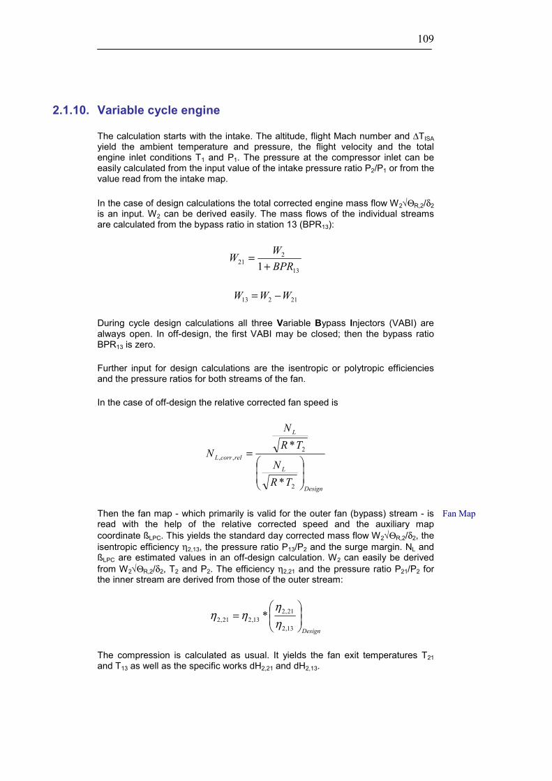
109
2.1.10. Variable cycle engine
The calculation starts with the intake. The altitude, flight Mach number and ∆TISA yield the ambient temperature and pressure, the flight velocity and the total engine inlet conditions T1 and P1. The pressure at the compressor inlet can be easily calculated from the input value of the intake pressure ratio P2/P1 or from the value read from the intake map.
In the case of design calculations the total corrected engine mass flow W2√ΘR,2/δ2 is an input. W2 can be derived easily. The mass flows of the individual streams are calculated from the bypass ratio in station 13 (BPR13):
13
221 1 BPR
WW+
=
21213 WWW −=
During cycle design calculations all three Variable Bypass Injectors (VABI) are always open. In off-design, the first VABI may be closed; then the bypass ratio BPR13 is zero.
Further input for design calculations are the isentropic or polytropic efficiencies and the pressure ratios for both streams of the fan.
In the case of off-design the relative corrected fan speed is
Design
L
L
relcorrL
TRN
TRN
N
=
2
2,,
*
*
Then the fan map - which primarily is valid for the outer fan (bypass) stream - is read with the help of the relative corrected speed and the auxiliary map coordinate ßLPC. This yields the standard day corrected mass flow W2√ΘR,2/δ2, the isentropic efficiency η2,13, the pressure ratio P13/P2 and the surge margin. NL and ßLPC are estimated values in an off-design calculation. W2 can easily be derived from W2√ΘR,2/δ2, T2 and P2. The efficiency η2,21 and the pressure ratio P21/P2 for the inner stream are derived from those of the outer stream:
Design
=
13,2
21,213,221,2 *
ηη
ηη
The compression is calculated as usual. It yields the fan exit temperatures T21 and T13 as well as the specific works dH2,21 and dH2,13.
Fan Map

110
DesignPPPP
PP
PP
−
−
−+=
1
1*11
2
13
2
21
2
13
2
21
Next is the calculation of the core driven fan stage, which is in effect the intermediate-pressure compressor (IPC). In the case of design calculations the pressure ratio and the efficiency are input values.
3 5312425
2
64
6
16
414
4445
13
163
637
98
b handling bleedoverboard bleeds
leakage from bypass
NGVCool.
HPT coolinga leakage to bypass
21 125
225
15
HP leak to LPT exit
baVABI 1
LPT cooling
VABI 3
VABI 2
VarCyc111RHCDPPT.WMF GasTurb
263
In off-design the IPC map is read with estimated values for the auxiliary coordinate ßIPC and the relative corrected speed of the intermediate spool:
Design
H
H
relcorrI
TRN
TRN
N
=
21
21,,
*
*
The exit station of the IPC is station 24. The corrected flow W21√ΘR,21/δ21, the pressure ratio P24/P21 and efficiency η21,24 are read from the map. Note that you must employ variable geometry with the core driven fan stage if one of the front VABI’s is closed in off-design simulations. The compression calculation yields T24, P24 and dH21,24.
The pressure at the inlet to the high-pressure compressor (HPC) is derived from the inter-duct pressure ratio P25/P24 for design calculations, whereas it depends on the corrected flow for off design calculations. There is no change in total temperature from station 24 to station 25.
Core driven fan stage

111
The second front VABI is located upstream of the high-pressure compressor. The mass flow through the open valve is given by the bypass ratio in station 15 (BPR15):
15
15215 1
*BPRBPR
WW+
=
Thus the core inlet mass flow is W25 = W2 - W15 and the mass flows into the bypass mixer are W125 = W24 - W25 and W225 = W15 - W125.
In an operating line calculation and during the simulation of the transient behavior you can select the handling bleed to be switched automatically. This bleed valve is closed if the relative corrected high-pressure compressor (HPC) speed is higher than NH,corr,rel,2. It will be open if the corrected speed is lower than NH,corr,rel,1. In between these boundaries then the handling bleed flow is interpolated linearly:
−−
−
=
1,,,2,,,
1,,,,,
max2525 1**
relcorrHrelcorrH
relcorrHrelcorrHHdlBldHdlBld NN
NNWW
WW
In off-design the HPC map is read with estimated values for the auxiliary coordinate ßHPC and the relative corrected speed:
Design
H
H
relcorrH
TRN
TRN
N
=
25
25,,
*
*
Now we look at the internal air system. The high-pressure turbine (HPT) cooling air mass flow is
=
25
,25, *
WW
WW HPTClHPTCl
This amount of cooling air is assumed not to do any work; it is mixed with the main gas stream behind the high-pressure turbine. The nozzle guide vane (NGV) cooling air mass flow is calculated in a similar manner:
=
25
,25, *
WW
WW NGVClNGVCl
The NGV cooling air is mixed with the main stream at station 41 upstream of the rotor(s), consequently this amount of air does work in the turbine. Leakages from the compressor exit to the bypass and to low-pressure turbine exit can also be taken into account:
=
25
,25, *
WW
WW BylkBylk
Handling Bleed
Internal air system

112
=
25
,25, *
WW
WW LPTlkLPTlk
The low-pressure turbine (LPT) needs also some cooling air
=
25
,25, *
WW
WW LPTClLPTCl
This air is often taken as an inter-stage bleed from the high-pressure compressor. Specific work done on this air is
3,25,, *dHfdH LPTClLPTCl =
The cooling air WCl,LPT is assumed not to do any work, it will be mixed with the main stream behind the LPT.
An overboard bleed mass flow can be specified as a linear combination of a relative and an absolute amount
2,25
1,25 * Bld
BldBld W
WW
WW +
=
The work done on the overboard bleed air is:
3,25*dHfdH BldBld =
For the compression of the NGV cooling air and the turbine rotor cooling air the specific power dH25,3 is required. The mass flow at the compressor exit W3 is the flow without the inter-stage bleeds that are not fully compressed (an inter-stage bleed is characterized by 0<fBld<1):
BldLPTCl WWWW −−= ,253
Between stations 3 and 31 the fully compressed bleed flows are subtracted:
LPTlkBylkHPTClNGVClHdlBld WWWWWWW ,,,,331 −−−−−=
The pressure loss in the burner is calculated as usual: in design calculations the pressure ratio P4/P3 is given, whereas in off-design calculations it is a function of the corrected flow and the design point pressure ratio.
The amount of fuel is calculated from the required fuel-air-ratio, which in turn depends on burner pressure, inlet temperature, humidity of the incoming air and temperature rise.
)(*/23134 OHf WWfarW −= η
The burner exit flow is W4=W31+Wf and the turbine nozzle guide vane exit flow W41 equals W4+WCl,NGV. The fuel-air-ratio far41 is
Burner

113
OHf
f
WWWW
far241
41 −−=
Now it is possible to calculate the enthalpy corresponding to the Stator Outlet Temperature (SOT) or Rotor Inlet Temperature (RIT) of the turbine:
413,4441 /)**( WHWHWH NGVCl+=
The power delivered by the high-pressure turbine (HPT) is a product of W41 and the specific power dH41,44. The energy balance with all power requirements, including the customer power offtake PWX, is given by
Hmech
BldBldLPTClLPTClmainHPC
WPWXdHWdHWPWdHW
dH,41
,,,24,212144,41 *
***η
++++=
PWHPC,main is the power needed to compress the main gas stream:
3,25,,,,31, *)( dHWWWWWWPW LPTLkByLkHPTClNGVClHdlBldmainC +++++=
If Turbine Design is selected then the isentropic efficiency of the HPT is calculated, otherwise, it is given as an input property. In off-design simulations the efficiency is read from the HPT map.
The relative corrected high-pressure turbine speed is
Design
H
H
relcorrHPT
TRN
TRN
N
=
41
41,,
*
*
The turbine efficiency and the corrected flow are read from the map with the known relative corrected spool speed and the auxiliary coordinate ßHPT. The efficiency can be modified in off-design simulations by a tip clearance correction term, which is a function of the relative mechanical spool speed:
HHclearancetip N
Nδδηη *)1( −=∆
From the specific work dH41,44 and the efficiency we can calculate P43=P44 and the turbine rotor exit temperature T43. Then the turbine rotor cooling air is added: W45=W41+WCl,HPT. The LPT inlet enthalpy H45 is calculated using the energy balance:
45
,34141414345
**),,(W
WHWwarfarThH HPTCl+
=
The fuel air ratio comes from
High pressure turbine

114
OHf
f
WWWW
far245
45 −−=
Pressure losses in the inter-duct between both turbines can be calculated in several ways. For design calculations, if turbine efficiency is taken from input, P45/P44 is a given quantity. If Turbine Design is selected and a value for the reference Mach number M44>0 is given, then the pressure loss will be adjusted according to the actual Mach number level. If the reference Mach number is not given, then the input value of P45/P44 is used again. During off-design the losses vary with the corrected flow in the same way as in any duct.
Normally, the low-pressure turbine (LPT) efficiency is an input value. However, efficiency can also be derived from turbine design calculations. The rotational speed of the LPT was calculated in the LPC Design section. The specific power required to drive the fan is
LmechWdHWdHW
dH,45
13,21321,22149,45 *
**η+
=
In the case of off-design the relative corrected speed of the LPT is
Design
L
L
relcorrLPT
TRN
TRN
N
=
45
45,,
*
*
The operating point in the map is determined by the estimated value of the auxiliary coordinate, ßLPT, and the relative corrected speed. Both the corrected flow, W45,std, and the efficiency are read from the map.
Now the LPT exit conditions, i.e., T49 and P5, can be calculated using the pressure ratio and efficiency. The cooling and leakage air will be mixed in the next step:
LPTLkLPTCl WWWW ,,455 ++=
OHf
f
WWWW
far25
5 −−=
5
4945,,,,5
***W
HWHWHWH LPTLkLPTLkLPTClLPTCl ++
=
The turbine exit duct pressure ratio P6/P5 can be found in the usual way. There is no change in the total temperature from station 5 to station 6.
From station 13 to 225 and from station 24 to 125 there are pressure losses that must be specified as P225/P13 and P125/P24 for the cycle design calculation. In off-design these pressure losses will vary with the corresponding corrected mass flows.
Turbine inter-duct

115
In station 15 the streams originating from stations 125 and 225 are mixed. In a design calculation either the Mach number Ma15 or the flow area A15 must be given. The mixer area A15 is split into A125 and A225 during the cycle design calculation in such a way that the static pressures Ps,125 and Ps,225 are equal. In off-design the static pressure balance between Ps,125 and Ps,225 is retained.
Downstream of the mixer there are additional pressure losses. These are specified as P16/P15 in a cycle design calculation and depend on corrected flow during off-design. The bypass exit mass flow is found from
ByLkHdlBldlkBy WW
WW
WW ,15
,1516 1* ++
−=
The inlet conditions for the cold side of the mixer are those from station 16. However, a nozzle cooling mass flow may first be subtracted from the bypass exit mass flow for engines with an afterburner:
−=
16
,1616163 *
WW
WWW NozCl
If the rear VABI is closed then all of the bypass air passes behind the cooling air liner of the afterburner.
If the rear VABI is open, then both the core and the bypass stream will be mixed. The hot stream mixer pressure ratio P63/P6 is assumed to vary with corrected flow in off-design simulations. The cold stream mixer pressure ratio P163/P16 is dependent on corrected flow in off-design, too.
The mixer area A64 is equal to the sum of A63 and A163. A64 can be specified by input or is calculated from the mean mixer Mach number M64 during design calculations. In off-design the static pressure balance between Ps,63 and Ps,163 is retained. The areas A63 and A163 are taken from the design point calculation. However, in off-design simulations you can also apply modifiers to the design point mixer areas to account for variable settings of the rear VABI. Note that in this case the total area A64 is recalculated as the sum of A63 and A163.
In the mixing calculation the program uses the conservation of energy for finding T64. The mass flow W64 is the sum of W6 and W161. P64 is calculated on the basis of conservation of momentum in a constant area duct.
Then the fuel-air-ratio far7 is calculated from the specified reheat exit temperature T7. Reheat fuel flow is then
−= 1*
64
7, far
farWW fRHf
The total reheat exit mass flow amounts to W7=W64+Wf,RH. The fundamental pressure loss caused by the heat addition will then be calculated. The correlations of the Rayleigh line, i.e., heat addition in a pipe with constant area, are used. The inlet Mach number for this calculation is M64.
Before the nozzle calculation starts, nozzle cooling air is mixed with the main stream. The nozzle total temperature will therefore be lower than T7, if nozzle cooling air is considered.
Mixer and afterburner

116
Two types of nozzles can be calculated: a convergent nozzle and a convergent-divergent nozzle with a prescribed nozzle area ratio A9/A8. The fully mixed net thrust for a convergent nozzle is
028,888, *)(*** VWPPACVWF ambsFGidN −−+=
For the convergent-divergent nozzle it is
029,998, *)(*** VWPPACVWF ambsFGidN −−+=
The pressure term A9*(Ps,9-Pamb) will be negative if the nozzle area ratio is too big for the pressure ratio.
These formulae apply to a fully mixed flow. However, in reality full mixing is not achieved. The thrust for a partially mixed flow is calculated on the basis of the separate expansion of W16 and W6 to ambient conditions. For a convergent nozzle the cold and hot stream gross thrusts are
)(*** ,16, ambcscFGccg PPACVWF −+=
)(*** ,6, ambhscFGhhg PPACVWF −+=
The areas Ac and Ah are calculated from continuity. The cold and hot stream thrust for a convergent-divergent nozzle is found in a similar matter. The partially mixed thrust is then calculated:
02,,, *)(*)1(* VWFFFF hgcgmixidgmixN −+−+= ηη
Note that in the case of reheat the mixing efficiency ηmix is set to 1.0 internally since combustion is assumed to enhance the mixing process.
Propulsion efficiency is
08
02Pr
**
1
2
VWVWFN
op ++
=η
Core efficiency is given by:
FHVWVdHW
f
iscore *
)2/(* 2045 −
=η
The enthalpy difference dHis is calculated assuming an isentropic expansion from the intermediate station 47 to ambient pressure. Station 47 is found by starting from station 45 and expanding the flow with the LPT efficiency to get the power needed for compressing the core flow W21 from P2 to P21.
For the mixed flow turbofan cycle you can get both a temperature-entropy and an enthalpy-entropy diagram. Often the region around station 2 will be very crowded. You should then enlarge this part of the graph.
Nozzle

117
2.1.11. Ramjet
The calculation starts with the intake. Altitude, the flight Mach number and ∆TISA provide the ambient temperature and pressure, the flight velocity as well as the total engine inlet conditions T1 and P1. P2 can easily be calculated from the input value of the intake pressure ratio P2/P1. Only design calculations are possible for the ramjet. The diffusor pressure ratio P6/P2 is an input quantity.
7 8 90 2 6 61
RamjetCDPPT.WMF GasTurb
Before burning the fuel the nozzle cooling flow is first subtracted from the total mass flow:
=
6
,6, *
WW
WW NozClNozCl
NozClWWW ,661 −=
The required amount of fuel is calculated from the fuel-air-ratio which in turn depends on burner pressure, inlet temperature and temperature rise.
)(*261
67
7OHf WW
farW −=
η
The total nozzle inlet mass flow is W7=W61+Wf. The fundamental pressure loss caused by the heat addition is then calculated by means of the Rayleigh line correlations, i.e., heat addition in a pipe with a constant area. The inlet Mach number M6 is an input value for this calculation. Before the nozzle calculation
Rayleigh line

118
starts, the cooling air is mixed with the main stream. The nozzle total temperature will therefore be lower than T7 if cooling is considered.
Two types of nozzles can be modeled: a convergent nozzle and a convergent-divergent nozzle with a prescribed nozzle area ratio A9/A8. Note, however, that the convergent-divergent nozzle subroutine will stop with an error message if the nozzle pressure ratio / nozzle area ratio combination implies a shock inside the nozzle.
The thrust for a ramjet with a convergent nozzle is
028888 *)(*** VWPPACVWF ambsFGN −−+=
For a convergent-divergent nozzle it is
029998 *)(*** VWPPACVWF ambsFGN −−+=
The pressure term A9*(Ps9-Pamb) will be negative if the nozzle area ratio is too big for the pressure ratio.
Propulsion efficiency of the ramjet is
08
02Pr
**
1
2
VWVWFN
op ++
=η

119
2.2. Details of the calculation
In this chapter you will find a description of the component calculations as performed in GasTurb. The same procedures are implemented in the program “GasTurb Details”.
2.2.1. Gas properties
The state of a thermodynamic system is described fully by two state variables. For example, enthalpy h may be written as a function of temperature and pressure:
),( PTfh =
The total differential of this relationship is
dPPhdT
Thdh
constTconstP ==
∂∂+
∂∂=
Specific heat at constant pressure is defined by
pconstP
cTh =
∂∂
=
The specific heat at constant pressure cP of a real gas depends on both temperature and pressure. Furthermore,
0≠
∂∂
=constTPh
For an ideal gas cp is constant and
0=
∂∂
=constTPh
We now introduce the half-ideal gas for which the following relations hold:
)(),( PfcTfc pp ≠=
0=
∂∂
=constTPh
Dry air behaves very much like a half-ideal gas at temperatures above approximately 200K.

120
The enthalpy of a half-ideal gas is
∫=T
Tp
ref
dTTcTh )()(
The reference temperature Tref can be selected arbitrarily. Its magnitude is not important for isentropic compression and expansion calculations because these involve only enthalpy differences.
For an isentropic process with a thermally ideal gas the following relationship holds
TdT
RTc
PdP p )(
=
In integral form this is
dTTTc
RPdP T
T
pP
P∫∫ =
2
1
2
1
)(1
We now define the entropy function Ψ as
dTTTc
RT
T
T
p
ref
∫=Ψ)(1)(
Again the reference temperature can be selected arbitrarily. Just as for the enthalpy, the calculation of isentropic compression and expansion processes uses only differences of entropy function values, not the absolute values themselves.
Use of the entropy function allows us to write the following simple formula for an isentropic change of state
121
2ln Ψ−Ψ=
PP
In gas turbines hydrocarbons are often used as fuel. Hydrocarbons composed of 86.08% carbon and 13.92% hydrogen (by mass) burn with air such that the molecular weight, and therefore also the gas constant of the combustion products, is exactly that of dry air R=287.05 J/(kg K). The lower heating value is 43.1 MJ/kg at T=288K. In GasTurb this type of fuel is called the Generic fuel.
Kerosene, JP-4 and other fuels used in aviation and in gas turbines for power generation are composed of hydrocarbons in such a way that their properties come close to that of the generic fuel described above. However, you can also select other fuels such as natural gas or hydrogen for your cycle calculation.
The chemical composition of natural gas can vary widely. For the calculation of the data used in GasTurb natural gas with 90%(by mass) CH4 and 10% C2H6 is considered.
Fuel and combustion products

121
The gas properties of air and combustion products are stored in tables that are read when a type of fuel is selected. These tables have been calculated with the NASA equilibrium code from Gordon McBride (ref. 15&16]. They contain data for the isentropic exponent, specific heat, molecular weight, enthalpy and entropy as a function of temperature, fuel-air-ratio and water-air-ratio.
For the evaluation of the isentropic exponent, the specific heat etc. the only species considered are N2, O2, H2O, CO2 and Ar. This guarantees that the composition of the combustion products is independent of pressure. All calculations in GasTurb, except those for combustion, are done for constant gas compositions. Allowing combustion products like CO or NOx while generating the gas property tables would cause erroneous calculation results.
The equilibrium temperature of the combustion process is stored as a function of fuel type, fuel-air-ratio, air temperature, pressure, humidity, water-fuel-ratio and steam-fuel-ratio. While calculating the equilibrium temperature there are no restrictions to the type of combustion products imposed, i.e. dissociation is taken into account.
The temperature of the fuel is 298.15K. The water temperature is the same while the steam temperature is assumed to be equal to the air temperature.
2.2.2. Intake
For the specification of the engine inlet conditions there are two options. With the Ground mode you can specify the total pressure P1 and the total temperature T1 upstream of the engine inlet as well as the ambient pressure surrounding the engine respectively the exhaust. With the Flight mode you specify altitude, deviation from standard atmosphere temperature and flight Mach number.
Given the flight altitude both static temperature and pressure are calculated using the international standard atmosphere (ISA). Below 11000m the ambient ISA temperature is
maltKT ISAamb 1000
*5.615.288, −=
Ambient pressure in this altitude range is
25588.5
1000*0225577.01*325.101
−=
maltkPaPamb
Between 11000m and 20000m the temperature is constant and equals 216.65K. Ambient pressure is
62.634111000
*632.22altm
amb ekPaP−
=
Ambient temperature for non-ISA days is Tamb= Tamb,ISA + ∆TISA. Extreme temperatures for cold and hot days are defined in MIL 210.
Flight mode

122
The velocity of sound depends on the static temperature and gas properties:
ambp
psonic TR
Rcc
V **−
=
The flight velocity V0 equals M0*Vsonic. Total temperature T0 is calculated from total enthalpy:
2)(
20
0VThH amb +=
An isentropic compression starting from Pamb gives P0:
)()(0
0* ambTTamb ePP Ψ−Ψ=
Since there is no energy transfer upstream of the first compressor, T2 equals T0. No pressure losses are assumed between stations 0 and 1. Therefore, P1 equals P0.
The intake pressure ratio P2/P1 is an input quantity. Positive values are used as they are, negative values are corrected for shock losses (supersonic flight only) according to MIL-E-5007:
[ ]35.1
1
2
1
2 )1(*075.01* −−
−= MPP
PP
input

123
2.2.3. Compressor design
The term “Compressor Design" in this program means to find compressor inlet dimensions and the rotational speed. These quantities are needed for inlet flow distortion and turbine design calculations and for transient simulations.
The input data are mass flow W, total pressure P, and temperature T. Tip speed uT, axial Mach number Max, and inlet radius ratio ν are also required. A minimum value for the hub diameter can furthermore be specified. This option is useful when different fan versions of a family of engines based on the same gas generator are to be studied.
From Max the static data Ps and Ts are found. The given mass flow requires a certain flow area, which implies a certain tip diameter for the given radius ratio. When the hub diameter calculated with this procedure is lower than the prescribed value then the radius ratio is recalculated based on the given hub diameter and the flow area. Angular velocity follows from blade tip speed.
The diameter of the engine inlet at the aerodynamic interface plane (AIP) is derived from the tip diameter of the first compressor. From that diameter one can calculate the flow area at the interface plane:
π*2
*2
,
,
= tipC
tipC
AIP dddAIP
The velocity head (ρ/2 V2)AIP will be used in the definition of the inlet flow distortion coefficient.
2.2.4. Compression
For a given inlet temperature T1, pressure ratio P2/P1 and efficiency η (isentropic or polytropic) the required specific work dH2,1 and the exit temperature T2 are calculated. First the entropy function for T1 is evaluated, and added to the logarithm of the pressure ratio:
+Ψ=Ψ
1
212 ln)()(
PPTT is
The inversion of the entropy function gives the isentropic exit temperature T2,is. Then the isentropic enthalpy rise is divided by the isentropic efficiency to give the effective specific work dH1,2.
η)()( 1,2
2,1
ThThdH is −
=
Polytropic and isentropic efficiency are related by
Aerodynamic Interface Plane

124
1
1
*1
1
2
1
1
2
−
−
= −
−
pol
PP
PP
isηγ
γ
γγ
η
This formula was used in previous versions of GasTurb to convert between the two efficiencies. Now polytropic efficiency is calculated as
=
1
,2
1
2
ln
ln
PPPP
ispolη
and isentropic efficiency as
)()()()(
12
1,2
ThThThTh is
is −−
=η
During cycle design calculations you can specify either polytropic or isentropic efficiency. Note, however, that any off-design calculations must follow a design point calculation in which all component efficiencies are specified as isentropic.
Isentropic efficiency may also be calculated as a function of stage loading and corrected flow. For this purpose the formulas for advanced technology compressors from ref. [11] have been implemented. The efficiency level can be adjusted with the help of the loss correction factor Kloss:
)1(*1 tan dardSlossK ηη −−=
2.2.5. Pressure losses
In design calculations the pressure ratio across a duct is normally taken as an input value. For turbine inter-ducts an additional option for the pressure loss calculation is available. When turbine design is selected, then the turbine exit duct inlet Mach number is calculated. The data for the duct pressure ratio can be specified for a reference Mach number. The actual pressure ratio then depends on duct inlet Mach number M. The loss coefficient ζ is defined as:
2
12
1
2
*2
11*1
ref
ref
M
M
PP
−
−+
−=
γγ
γ
ζ
The actual pressure ratio for the duct inlet Mach number M is then
Polytropic and isentropic efficiency

125
12
2
1
2
*2
11
*1−
−+
−=γγ
γζ
M
MPP
In off-design calculations duct losses are dependent on the relative corrected flow:
Design
Design
PP
PTRW
PTRW
PP
−
−=
1
2
2
1
2 1***
**1
A special case is the pressure loss due to heat addition. This loss is neglected in the main burner. In reheat systems the pressure losses are calculated from the Rayleigh line, i.e., a constant area duct without friction is assumed and from conservation of momentum the pressure loss is found.
Another special case is the pressure loss due to mixing. It is only taken into account for the mixing of core and bypass streams, and not for the mixing of cooling or leakage air with the mainstream.
2.2.6. Combustion chamber
Efficiency
Modern combustion chambers have at design condition very high efficiency, at part load near idle and at very high altitude, however, the burner efficiency can deviate noticeable from 100%.
Burner efficiency can be correlated with burner loading which is defined as
VolePW
KT ** 300/8.13
313
=Ω
where Vol is the burner volume.
For the cycle design point in GasTurb the burner efficiency is an input property and the burner loading is by definition equal to 100%. For part load conditions the relative burner loading Ω/Ωdp can be determined without knowing the burner volume because the volume is invariant.
In literature it can be found that the change in burner efficiency with load can be approximated by
ΩΩ+=−dp
ba log*)1log( η

126
The constant a in this formula is correlated with the design point efficiency:
)1log( dpa η−=
Thus it is possible to describe the burner part load efficiency trend with a single property, the burner part load constant b. Both the design point efficiency and the part load constant have an influence on the burner efficiency.

127
Pressure loss
There are two reasons for pressure losses in combustion systems: friction and heat addition. Pressure losses due to friction are given as pressure ratio P4/P3 in the cycle design point. During off-design simulations the pressure losses vary proportional to corrected burner inlet flow squared.
Pressure losses due to heat addition are neglected in the main burner because the Mach number there is very low. In reheat systems the pressure losses are calculated from the Rayleigh line, i.e., a constant area duct without friction is assumed and from conservation of momentum the pressure loss is found.
Emissions
The combustion products of hydrocarbon fuel with air are mainly water and carbon dioxide. Thus the emission of CO2 is directly coupled to the fuel consumption of a gas turbine.
At full load additionally nitrogen oxides NOx are produced while at part power carbon monoxide CO and unburned hydrocarbons UHC are the problem.
The production of nitrogen oxides increases with pressure, temperature and residence time in the combustor while water in the combustion air reduces the amount of nitrogen oxides. The NOx severity parameter is defined as
−+
−
= 2.53
*10029.6194
8264.03
3
*2965
warKKT
NO ekPaPS
x
The NOx Emission Index EI [g/kg fuel] increases linearly with the NOx severity parameter. For conventional combustors holds
xNOSEI *32≈
while for dual annular combustors the NOx emission is approximately
xNOSEI *23≈
Consequently, reduction techniques focus on just what latitude one has with these variables in view of the engine cycle requirements. Not only is temperature the most sensitive of these, but owing to the design of conventional burners, it also offers the greatest possibility for control. In the conventional engine, fuel is initially burned at approximately stoichiometric conditions and subsequently diluted to the desired leaner condition. The high temperatures in the primary combustion zone result in rapid production of NOx during its residence time and set the value of the final emission level. The advantages of this arrangement are that the hot, stoichiometric primary zone provides good stability, ignition and relight, while the addition of dilution air allows convenient cooling of the combustor liner.

128
The low-NOx burners are consequently designed to avoid the hot stoichiometric and dilution zones, thereby reducing emissions, but at the expense of stability and cooling problems.
Incomplete combustion results in the production of carbon monoxide CO and unburned hydrocarbons UHC. The amount of these species can be correlated with the combustion (in)efficiency:
( )UHCCO EIEI +=− *232.0*1.0100*)1( η
There is a relationship between the two emission indices:
21 )log(*)log( cEIcEI COUHC +=
Data from an extensive measurement campaign with the CFM56 engine correlate well when c1 = 3.15 and c2 = - 4.3 are used in this formula, for example.
2.2.7. Turbine design
A preliminary turbine design may be selected. Turbine geometry and efficiency calculations are performed on a mean section basis assuming symmetrical diagrams for each stage (except the first stage, which has axial inlet flow).
Figure 1: Turbine velocity triangles and Smith diagram
The method used is a simplified version of the NASA program published as ref. [3]. The details cannot be described in this manual. Some advice with respect to the input and output is given below.

129
The first input is the number of turbine stages (maximum 10). Then the inlet radius ratio (a number less than 1) must be given. It is defined at the exit of the first rotor. Obviously for one-stage turbines the exit radius ratio is the same as the inlet radius ratio. Inlet and exit mean diameters are defined at the same location as the radius ratios. For one-stage turbines both values are again the same. The next quantity that must be input is the axial velocity ratio, which is the ratio of exit axial velocity to mean axial velocity.
The efficiency calculated by the program can be adapted to any technology level by adjusting the loss coefficient Kloss. The NASA report proposes a value for Kloss in the range of 0.35 to 0.4. The large uncooled turbines of modern engines are better described with values as low as 0.3.
Another method may also be used for adjusting the efficiency level. Especially in small engines the tip clearance can be - expressed in relative blade height - quite large. The tip clearance and the exchange rate for efficiency with relative tip clearance (a typical value is 2) can be input after selecting tip clearance corrections by a separate switch.
Figure 2: Cooling air constant
The reference Mach number for calculating the turbine inter-duct loss between a high and a low-pressure turbine (see preceding chapter) is another value that must be input. If it is set to zero, then the input value for the inter-duct pressure ratio will be used.
For the calculation of blade metal temperature the cooling effectiveness must be known. It may be found using the following equation (ref. [2]):
coolrefcl
refclcool CWW
WW+/
/η
The cooling air constant Ccool (range: 0.03 to 0.07) has to be adjusted to get reasonable results. Metal temperature is calculated from
)(* aircoolingrelcoolrelMetal TTTT −−= η

130
As a measure for blade stress the product of area times speed squared is employed. Its value found from
6222 10**1
1*** −
+
−= RPM
dddd
dNA
o
i
o
i
meanπ
Flow angles are measured relative to the turbine axis. Positive angles are in the direction of rotation. You will get useful results for the efficiency from turbine design only for a limited range of input data. The diameters needed for input can be estimated from compressor calculations: a good first estimate for the mean HPT turbine inlet diameter is the HPC inlet tip diameter.
2.2.8. Expansion
For a given inlet temperature T1, specific work dH 1,2 and efficiency η (isentropic or polytropic) the pressure ratio P1/P2 and the exit temperature T2 are calculated. First the isentropic specific work is found from specific work and isentropic efficiency. This gives the isentropic exit temperature T2,is:
isis
dHThTh
η2,1
1,2 )()( −=
The difference in the entropy functions for T1 and T2,is is equal to the logarithm of the pressure ratio. From this it follows that
)()(12
1,2* TT isePP Ψ−Ψ=
The exit temperature is found easily by using the enthalpy H2=H1-dH1,2. Polytropic and isentropic efficiencies are related by
1
1
1
2
1
1
2
1
−
−
= −
−
γγ
γγη
η
PP
PP pol
is
This formula was used in previous versions of GasTurb to convert between the two efficiencies. Now polytropic efficiency is calculated as
=
2
1
,2
1
ln
ln
PP
PP
ispolη
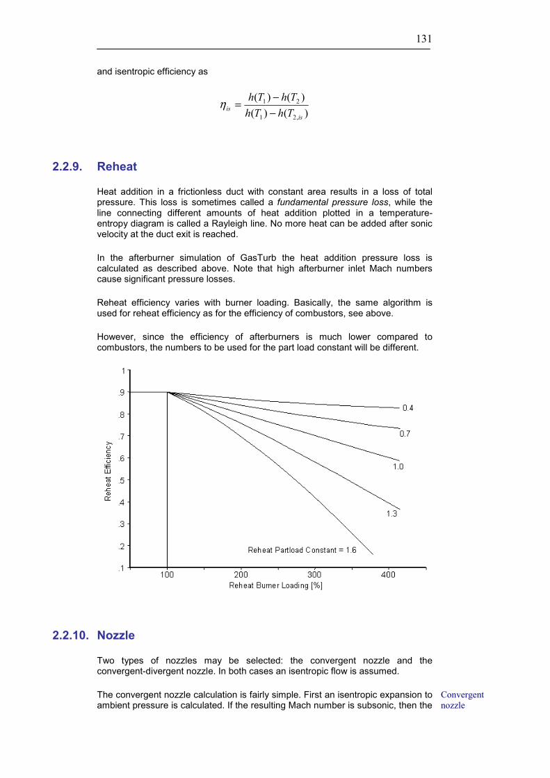
131
and isentropic efficiency as
)()()()(
,21
21
isis ThTh
ThTh−−
=η
2.2.9. Reheat
Heat addition in a frictionless duct with constant area results in a loss of total pressure. This loss is sometimes called a fundamental pressure loss, while the line connecting different amounts of heat addition plotted in a temperature-entropy diagram is called a Rayleigh line. No more heat can be added after sonic velocity at the duct exit is reached.
In the afterburner simulation of GasTurb the heat addition pressure loss is calculated as described above. Note that high afterburner inlet Mach numbers cause significant pressure losses.
Reheat efficiency varies with burner loading. Basically, the same algorithm is used for reheat efficiency as for the efficiency of combustors, see above.
However, since the efficiency of afterburners is much lower compared to combustors, the numbers to be used for the part load constant will be different.
2.2.10. Nozzle
Two types of nozzles may be selected: the convergent nozzle and the convergent-divergent nozzle. In both cases an isentropic flow is assumed.
The convergent nozzle calculation is fairly simple. First an isentropic expansion to ambient pressure is calculated. If the resulting Mach number is subsonic, then the
Convergent nozzle

132
static conditions in the nozzle exit plane have already been found. Otherwise the nozzle exit Mach number is set to 1.0, and using this condition we obtain new values for Ts,8 and Ps,8.
Discharge coefficient
The correlation between the effective flow area Aeff,8 and the geometric nozzle area A8 is described by the nozzle discharge coefficient CD,8 = Aeff,8/A8. The magnitude of this coefficient depends on the nozzle petal angle α and the nozzle pressure ratio P8/Ps,8.
GasTurb approximates the discharge coefficient of real nozzles with the empirical correlation as shown in the figure. Note that you can achieve CD,8=1 by setting the design nozzle petal angle to zero.
During off-design simulations the petal angle is found from the geometric nozzle area A8.
For the convergent-divergent nozzle the calculation from the inlet to the throat (station 8) is normally an expansion to sonic conditions. From station 8 to station 9 the flow is expanded supersonically in accordance with the given area ratio A9/A8. If the nozzle exit static pressure Ps,9 is higher than ambient pressure then the solution has been found and the calculation is finished.
Otherwise, a vertical shock is calculated using the upstream Mach number M9. When the static pressure downstream of the shock is lower than ambient pressure, there will be a shock inside the divergent part of the nozzle. If not, then the pressure term in the thrust formula is negative; however, the result with Ps9 less than Pamb is valid.
At very low nozzle pressure ratios the flow will be completely subsonic. In such cases the nozzle behaves like a venturi.
Convergent-divergent nozzle

133
With the help of the program GasTurb Details you can study in detail all the flow phenomena that can occur within a convergent-divergent nozzle.
For convergent-divergent nozzles the ideal thrust coefficient cV9 is calculated by relating the actual thrust to the ideal thrust of a convergent-divergent nozzle. The latter has the optimum area ratio A9/A8, i.e., it expands the flow exactly to ambient pressure.
The mass flow through a convergent-divergent nozzle is calculated using the formulas for a convergent nozzle. This is not correct for subcritical pressure ratios, but it is a much simpler calculation.
The geometry of a convergent divergent nozzle is described with the primary petal angle and the area ratio A9/A8.
The mechanical design of a convergent-divergent nozzle is often such that the nozzle area ratio A9/A8 changes when the nozzle throat area A8 is modulated. To describe this, during off-design simulations the area ratio A9/A8 can be made a function of A8.
2
,8
8
,8
8
8
9 **
++=
dsds AAc
AAba
AA
When you only want to do cycle design point calculations, then set a to the desired nozzle area ratio and set both b and c to zero.
2.2.11. Propeller
From GasTurb you will get information about an ideal propeller and a real propeller. For the real propeller you can use a map and thus accurately describe the behavior of this device.
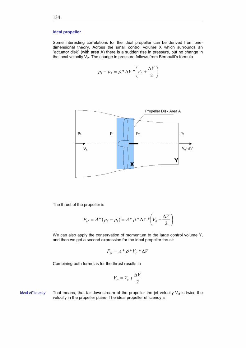
134
Ideal propeller
Some interesting correlations for the ideal propeller can be derived from one-dimensional theory. Across the small control volume X which surrounds an “actuator disk” (with area A) there is a sudden rise in pressure, but no change in the local velocity VP. The change in pressure follows from Bernoulli’s formula
∆+∆=−
2** 021
VVVpp ρ
V0
p1 p2p0 p0
V0+∆V
Propeller Disk Area A
YX
The thrust of the propeller is
∆+∆=−=
2***)(* 012
VVVAppAFid ρ
We can also apply the conservation of momentum to the large control volume Y, and then we get a second expression for the ideal propeller thrust:
VVAF Pid ∆= *** ρ
Combining both formulas for the thrust results in
20VVVP
∆+=
That means, that far downstream of the propeller the jet velocity Vid is twice the velocity in the propeller plane. The ideal propeller efficiency is
Ideal efficiency

135
)(***
12
0, ppVA
VF
P
ididP −
=η
which can be transformed to
0
,
1
2
VVid
idP
+=η
The ideal thrust coefficient is a measure of thrust per unit of propeller disk area:
AV
FC id
idF
**2
20
, ρ=
Another propeller performance indicator is the ideal power coefficient, which is defined as
AV
ppVAC PidPW
**2
)(**3
0
12, ρ
−=
Real propeller
In reality there are always losses like frictional drag on the blades, uneven velocity distribution over the propeller disk area, swirl in the slipstream etc. Therefore, the performance of a real propeller will never be as good as that of an ideal propeller.
Traditionally the performance of real propellers is described by some dimensionless parameters, see Ref. [6]. The thrust coefficient is
42 ** dnFCF ρ
=
with n = rotational speed (in revolutions per second) and d = propeller diameter.
The quantity V0/(n*d) is known as the advance ratio J. It is a measure of the forward movement of the propeller per revolution.
There is the power coefficient CPW defined as
53 ** dnPW
C SDPW ρ
=
The efficiency of the propeller is
Ideal thrust coefficient
Ideal power coefficient
Thrust coefficient
Advance ratio
Power coefficient
Propeller efficiency

136
PW
F
SDP C
JCPWVF ** 0 ==η
For static conditions (J=0) this definition leads to ηP = 0. In this case the following definition of the propeller quality is appropriate (Ref. [6]):
PW
FstaticP C
C 2/3
, *2π
η =
From the cycle calculation the shaft power delivered, PWSD, is known and the power coefficient of the propeller can be calculated easily. The static thrust follows from
42
3/2
, ***2
* dnC
F PWstaticPstatic ρ
π
η
=
The ratio of thrust coefficient to power coefficient CF/CPW is another measure of static propeller efficiency. From this ratio you can also calculate the static thrust:
dnPW
CCF SD
PW
Fstatic *
*=
When you do not use a propeller map with GasTurb, then the input value for the propeller efficiency is interpreted as ηP for V0>0 and as ηP,static in the case of static conditions.
You can also use a propeller map that will give you the efficiency as a function of the advance ratio and the power coefficient. For static conditions an additional correlation is stored in a separate table as CF/CPW = f (CPW).
The propeller map is difficult to read in the region of low advance ratios. There the thrust will be linearly interpolated between the static thrust and the value derived from ηP for an advance ratio of 0.2.
The propeller efficiency read from the map can be corrected for Mach number effects. Above the critical Mach number, efficiency will drop according to
2)(* critP MMC −=∆ ∆ηη
When you do not have a map of the propeller which fits to your engine design point, then you can scale the map delivered with the program.
Static efficiency
Propeller map

137
Figure 3: Propeller map
When designing a turboprop engine the question arises as to what ratio of propeller thrust to residual jet thrust is best. As shown for example in ref. [1], the optimum velocity ratio is
PmechLPTopt
VV
ηηη **0
,8 =

138

139
2.3. Iteration technique
2.3.1. Mathematical background
The calculation of each off-design point requires an iteration. Several input variables for the thermodynamic cycle must be estimated. The result of each pass through the cycle calculations is a set of "errors". Inconsistencies in the aero-thermodynamics are introduced through the use of imperfect estimates for the variables. The number of errors equals the number of variables.
The algorithm used to manipulate the variables in such a way that in the end all errors will be insignificant is a Newton-Raphson iteration. With two variables Vj and two errors Ei this algorithm works as follows.
First the variable V1 is changed by the small amount of ∂V1. Both errors E1 and E2 will change, and we will get the influence coefficients ∂E1/∂V1 and ∂E2/∂V1. Then V1 is reset to its original value and the second variable V2 is changed by ∂V2. Again both errors will change and we will get ∂E1/∂V2 and ∂E2/∂V2.
Let us assume for the moment that the influence coefficients ∂Ei/∂Vj are constant. Then we can immediately calculate how the variables Vj need to be changed to reduce the errors Ei to zero:
122
11
1
1 EVVEV
VE
−=∆∂∂
+∆∂∂
222
21
1
2 EVVEV
VE
−=∆∂∂
+∆∂∂
In reality, the influence coefficients are not constant and these changes of the Vj will not directly lead to Ei=0 after this single correction.
The algorithm can be applied to any number of variables. The matrix of influence coefficients is called the Jacobi matrix. The system of linear equations is solved by means of the Gauss algorithm.
A numerical example involving two variables illustrates the iteration technique. Let’s look at the following linear relationships:
435 211 ++= VVE
2473 212 ++−= VVE
We are looking for the set of variables that reduces both errors E1 and E2 to zero. Let us guess and set V1 =3 and V2 =7. By checking the equation we find that E1=40 and E 2=64. Now the Newton-Raphson iteration is started. First the partial derivatives needed to create the Jacobi matrix are calculated:
51
1 =∂∂VE
32
1 =∂∂VE
Newton-Raphson
Jacobi matrix

140
31
2 −=∂∂VE
72
2 =∂∂VE
The changes needed to reduce both E1 and E 2 to zero can then be calculated as follows:
4035 21 −=∆+∆ VV
6473 21 −=∆+∆− VV
The solution to this system of linear equations is ∆V1= -2 and ∆V2= -10. The new values for the iteration variables are then V1 = 3 - 2 = 1 and V2 = 7 - 10 = -3. When we insert these values into the equations for E1 and E2 we will see that both E1 and E2 are zero as desired.
In the previous example the relation between the variables and the errors was linear. We now try the following quadratic functions as an exercise:
540025153075 212
22
11 −−−−= VVVVE
48005039213 212
22
12 −+++−= VVVVE
We start with V1=11 and V2=3. After creating the Jacobi matrix and solving the linear equation the improved estimates are V1=6.944 and V2=-2.929. The exact solution is V1=7 and V2=-3.
GasTurb marks the iteration variables as estimated values in the off-design input data notebook. You can thus distinguish them from the normal input data. Reasonable estimates are required for the iteration variables. If the estimates are too far away from the solution, the program may have convergence problems. In this case you must make several intermediate steps from the design point toward the desired off-design operating condition.
Besides the normal cycle data the output for each off-design point contains the number of iteration loops used. If the iteration has not converged, then the sum of the square of the iteration errors ΣError²=ΣEi² is also shown. The last digit of ΣError² will be zero or one after full convergence. If GasTurb fails to achieve full convergence (ΣError²>10-8), it will show the point with the smallest ΣError² encountered during the iteration process. Such a solution will be quite acceptable most of the time.
In the case of non-convergence it may help to restart the iteration. GasTurb changes the step size for calculating the Jacobi matrix, i.e. the ∂Vj, randomly, so that repeating the iteration may yield a better result than before.

141
2.3.2. Single spool turbojet
Let us go through an off-design calculation with a given rotational speed. We will find the variables and the errors mentioned in the previous section. The sequence of the calculations is outlined.
The calculation starts with the inlet. This provides the compressor inlet conditions. The compressor map has to be read next. Although we know the aerodynamic speed N/√ΘR2, this is not sufficient to place the operating point in the map. An estimate for the auxiliary coordinate ßC is required. ßC is our first variable.
We can read the mass flow, the pressure ratio and the efficiency from the compressor map and calculate burner inlet conditions. The amount of fuel required running the engine at the specified rotational speed is still unknown. An estimate for the burner exit temperature T4 will yield the fuel-air-ratio. T4 is the second variable.
The combustor exit mass flow W4 is derived from the compressor exit flow W3, the internal air system (cooling air, bleed) and the fuel flow WF. The pressure loss in the burner depends on the corrected burner inlet flow only. It's no problem to find the total pressure at the burner exit P4. We can directly calculate the corrected flow W4√ΘR4/δ4 at the inlet to the turbine.
Selecting the turbine operating point is similar to selecting that of the compressor: we know the corrected speed N/√ΘR4, but not the value of the auxiliary map coordinate for reading the turbine map. ßT is the third variable we have to estimate.
Reading the turbine map provides us with the corrected flow (W4√ΘR4/δ4)map and the efficiency. Here the corrected flow is derived from a second source. The difference between both corrected flows constitutes the first error of our iteration.
We will ignore this error for the moment and go on. The turbine exit conditions and the shaft power produced are calculated using the values read from the map. The difference between the power required driving the compressor and the power produced by the turbine (it is obvious that they must be equal to ensure steady state operation) is the second error of the iteration.
The pressure loss (P5-P6)/P5 in the turbine exit duct depends only on the corrected flow. When reheat is not switched on then P6 equals the nozzle total pressure P8. Furthermore W8 equals W6 and T8 equals T6. Thus the nozzle inlet conditions are fully fixed.
A certain total pressure P8,req is required to force the flow W8 with the total temperature T8 through the given area A8, while the back pressure is equal to Pamb. As long as the iteration has not yet converged there will be a difference between P8 and P8,req. This constitutes the third error of the iteration.
We have found three variables and three errors. The Newton-Raphson iteration algorithm modifies the variables in such a way that all errors equal zero.
The above explanation applies when the compressor rotational speed is specified. Alternatively the burner exit temperature T4 can be specified. In this case the first variable will be the spool speed instead of T4; the calculation procedure and the iteration errors will remain the same.
Estimate ßC
Estimate T4
Estimate ßT
Turbine flow error
Turbine work error
Nozzle inlet pressure error

142
When limiters are active then an additional error is generated, i.e., the deviation from one of the specified limiting values. We now need an additional variable, and therefore we use both the compressor rotational speed and the burner exit temperature T4 as estimated values.
GasTurb calculates the deviations for all limiters. The limiter errors are formulated in such a way that any value higher than the limiter setting results in a positive number. The selection of the biggest error out of all limiter errors ensures that no value will exceed its limit after convergence. The biggest error - which is nearly zero - defines the active limiter.
The Limiters option also makes it possible to run an off-design cycle for a specified thrust or fuel flow while reheat is switched off. Here you first need to define the composed value number 20 as the net thrust or as fuel flow. You enter your target number on the limiter page of the tabbed notebook and start the off-design calculation.
If you have also switched on other limiters, you can for example get a solution for the following problem: "I want x kN thrust if the turbine inlet temperature is below y K and the compressor speed is less than or equal to z%."
If reheat is selected the calculation described above will be done first. Reheat fuel will not be taken into account until the iteration converges. GasTurb uses an equivalent dry nozzle area during this part of the calculation. After convergence the afterburner is switched on. The calculation restarts in station 6, with new nozzle inlet conditions. These new conditions require a certain area A8 in order that the flow can pass through the nozzle. The output screen displays the result of this recalculated area. If you wish to study the effect of different nozzle areas on the reheated performance, you need to modify the equivalent dry nozzle area by entering a value of, say, 5% for Delta Nozzle Area.
Since reheat is calculated only after the iteration has converged, it is not possible to iterate for a given thrust or fuel flow while reheat is switched on. The problem is ambiguous, as reheat thrust depends on both the turbomachinery performance and the reheat exit temperature. You must vary the input value of the reheat exit temperature to get a thrust at a constant dry engine rating.
2.3.3. Two-spool turboshaft, turboprop
In GasTurb the setup of the off-design iteration for the two-spool turboshaft resembles that of the turbojet. Up to the high-pressure turbine exit the procedure remains the same. The first variable is the auxiliary coordinate ßC which is used to read the compressor map. The second variable is either the rotational speed NH of the compressor or the burner exit temperature T4. The third variable is the auxiliary coordinate ßHPT needed to read the map of the high-pressure turbine.
The burner exit corrected flow will not be equal to the HPT corrected flow as long as the iteration has not yet converged. The difference between both corrected flows constitutes the first error of our iteration.
The high-pressure turbine (HPT) exit conditions and the shaft power produced are calculated using the values read from the map. The difference between the power required driving the compressor and the power produced by the turbine (it is obvious that they must be equal to ensure steady state operation) is the second error of the iteration.
Reheat
Estimate ßC, NH or T4 and ßHPT
HPT flow error
HPT work error

143
We ignore this error for the moment and go on. The HPT exit conditions are derived from the power required to drive the attached compressor and from HPT efficiency. It is no problem to find the turbine inter-duct pressure loss. We can directly calculate the low-pressure turbine inlet corrected flow.
Selecting the low-pressure turbine operating point is similar to selecting that of the compressor: we know the corrected speed NL/√ΘR45 for reading the LPT map, but not the value of the auxiliary map coordinate. ßLPT is the forth variable that we have to estimate.
Reading the turbine map provides us with the corrected flow (W45√ΘR45/δ45)map as well as the LPT efficiency. Here the corrected flow is derived from a second source. The difference between both corrected flows constitutes the second error of the iteration.
We will ignore this error for the moment and go on. The turbine exit conditions and the shaft power delivered are calculated by means of the values read from the map.
The pressure loss (P5-P6)/P5 of the turbine exit duct depends only on the corrected flow. P6 is equal to the total pressure within the nozzle, P8. Furthermore W8 equals W6 and T8 equals T6. The nozzle inlet conditions are thus fully determined.
A certain total pressure P8,req is required to force the flow W8 with the total temperature T8 through the given area A 8, while the back pressure is equal to Pamb. As long as the iteration has not yet converged, there will be a difference between P8 and P8,req. This constitutes the forth error of the iteration.
We have found four variables and four errors. The Newton-Raphson iteration algorithm modifies the variables in such a way that all errors equal zero.
If limiters are used, then an additional error will occur, i.e. the deviation from one of the specified limiting values. An additional variable is required. Without limiters either NHPC or T4 can serve as a variable, but with limiters both NHPC and T4 are variables.
GasTurb calculates the deviations for all limiters. The limiter errors are formulated in such a way that a value higher than the limit results in a positive number. The selection of the biggest limiter error ensures that after convergence no limiter will be exceeded. The biggest error - which is nearly zero - defines the "active limiter".
The limiter option also makes it possible to run an off-design cycle for a specified shaft power or fuel flow. You first need to define the composed value number 20 as the shaft power or as the fuel flow. You enter your target number in the limiter-input menu and start the off-design calculation.
If you have switched on other limiters simultaneously, you can, for example, get a solution to the following problem: "I want x kW power provided that the turbine inlet temperature is below y K and the compressor speed NH is less or equal to z%."
Estimate ßLPT
LPT flow error
Nozzle inlet pressure error
Prescribed shaft power or fuel flow

144
2.3.4. Boosted turboshaft, turboprop
For this type of engine, the low-pressure spool speed NL is an input quantity. The booster map auxiliary coordinate ßIPC must be estimated; it is the first variable of the iteration. The inlet conditions and the data read from the map yield W2, T24 and P24.
After the compressor inter-duct, the mass flow is reduced by the handling bleed, and W25 equals W24 - WHdlBld. Total temperature does not change, and the pressure loss can be calculated easily. The corrected mass flow in station 25 is now known. Next the HP compressor map is read using NHPC (which is either specified or estimated) and ßHPC yielding another value for the corrected flow: (W25√ΘR25/δ25)map. The difference between those two flows constitutes the first error of the iteration.
We find two turbine mass flow errors, the HPT work error and the nozzle inlet pressure error, as in the case of the two-spool turboshaft. The iteration scheme consists of the following variables and errors:
variable error ßIPC HP compressor mass flow NHPC HPT mass flow ßHPC HPT work ßHPT LPT mass flow ßLPT nozzle inlet pressure
This assumes that NHPC is a specified value. In the alternative procedure T4 is specified, and NHPC is a variable for the iteration instead of T4. When limiters are used, the other variable is also employed giving a total of six errors and six variables.
2.3.5. Unmixed flow turbofan
The iteration starts with estimated values for the rotational speed of the low- pressure spool NL and for the auxiliary coordinate ßLPC. This allows us to read the fan (LPC) map. The inlet conditions and the data read from the map yield T21, P21, T13 and P13. The total mass flow W2 is also derived from the map. We need to split this mass flow between the core and the bypass streams and estimate the bypass ratio, which constitutes the third variable of the turbofan iteration.
Core stream calculations will be done next. The compressor inter-duct pressure loss depends only on W21√ΘR21/δ21. After subtracting the handling bleed flow WHDBld, we can find the corrected flow W25√ΘR21/δ25 at the high pressure compressor (HPC) inlet.
Let us assume that the rotational speed of the high-pressure spool NH is specified. To read the HPC map we need an estimate for the auxiliary coordinate ßHPC, which constitutes our fourth variable.
The pressure ratio P3/P25, efficiency ηHPC and the corrected flow (W25√ΘR25/δ25)map can be read from the map. The difference between this corrected flow and the one calculated before constitutes the first error of the turbofan iteration.
Estimate NL, ßLPC and bypass ratio
Estimate ßHPC
HPC flow error

145
We will ignore this error and calculate the burner inlet conditions by means of the values read from the HPC map. Burner exit temperature T4 is an estimated value, the fifth variable of the iteration.
Selecting the turbine operating point is similar to selecting that of the compressor: we know the corrected speed NH/√ΘR4, but not the value of the auxiliary map coordinate for reading the high-pressure turbine map. ßHPT is the sixth variable we have to estimate.
The burner exit corrected flow will not be equal to the HPT corrected flow as long as the iteration has not yet converged. The difference between both corrected flows constitutes the second error of our iteration.
The high-pressure turbine (HPT) exit conditions and the shaft power produced are calculated using the values read from the map. The difference between the power required driving the high-pressure compressor and the power produced by the HPT (it is obvious that they must be equal to ensure steady state operation) is the third error of the iteration.
We will ignore this error for the moment and go on. The HPT exit conditions are derived from the power required to drive the high pressure compressor and from HPT efficiency. It presents no problem to find the turbine inter-duct pressure loss. We can directly calculate the low-pressure turbine inlet corrected flow W45√ΘR45/δ45.
Selecting the low pressure turbine operating point is similar to selecting that of a compressor: we know the corrected speed NL/√ΘR45, but not the value of the auxiliary map coordinate used for reading the LPT map. ßLPT is the seventh variable which we have to estimate.
Reading the turbine map provides us with the corrected flow (W45√ΘR45/δ45)map and the LPT efficiency. Here the corrected flow is derived from a second source. The difference between these corrected flows constitutes the forth error of the iteration.
As usual we will ignore this error for the moment and proceed. The turbine exit conditions and the shaft power delivered are calculated using the values read from the map. The difference between the power required to drive the low- pressure compressor (fan) and the power delivered by the LPT (it is obvious that they must be equal to ensure steady state operation!) yields the fifth error of the iteration.
The pressure loss (P5-P6)/P5 of the turbine exit duct depends only on the corrected flow W5√ΘR5/δ5. P6 is equal to the total pressure P8 in the core nozzle. Furthermore, W8 is equal to W6 and T8 is equal to T6. The core nozzle inlet conditions are thus fully fixed.
A certain total pressure P8,req is required to force the flow W8 which has the total temperature T8 through the given area A8, while the back pressure is equal to Pamb. As long as the iteration has not yet converged there will be a difference between P8 and P8,req. This difference constitutes the sixth error of the iteration.
We now go on with the bypass stream. Its pressure loss depends only on the bypass inlet corrected flow. P18, T18 and W18 define secondary nozzle inlet conditions. Analogously to the core nozzle procedure we can calculate the pressure P18,req which is required to force the flow through the given area A18. P18 will not be equal to P18,req during the iteration. This constitutes the seventh error.
Estimate T4
Estimate ßHPT
HPT flow error
HPT work error
Estimate ßLPT
LPT flow error
LPT work error
Core nozzle inlet pressure error
Secondary nozzle pressure error
146
We have found seven variables and seven errors. The Newton-Raphson iteration algorithm modifies the variables in such a way that all errors equal zero.
The limiter option also makes it possible to run an off-design cycle for a specified thrust or fuel flow. You first need to define the composed value number 20 as the net thrust or as the fuel flow. You enter your target number in the limiter-input menu and start the off-design calculation.
If you have switched on other limiters simultaneously, you can get a solution to the following problem: "I want x kN thrust provided that the turbine inlet temperature is below y K and the HP compressor speed is less than or equal to z%."
2.3.6. Mixed flow turbofan
The iteration for a mixed turbofan is very similar to that for an unmixed turbofan, as described in the previous chapter. It leads to the same variables, and all the errors are the same except one. We obviously have to replace the error derived from continuity in the secondary nozzle.
The seventh error for the mixed turbofan is the difference between the static pressures Ps63 and Ps163 in the mixing plane.
2.3.7. Geared Turbofan
The iteration for the geared turbofan is also very similar to that described for the unmixed turbofan. The difference is in the additional intermediate pressure compressor (IPC). Its rotational speed is easily derived from NL, since it is connected to the fan mechanically. We must, however, make an estimate for the auxiliary coordinate ßIPC in addition to the seven variables of the unmixed turbofan.
There is also an additional error: The corrected flow W21√ΘR21/δ21 downstream of the low pressure compressor (fan) will not be the same as the value read from the IPC map (W21√ΘR21/δ21)map.
There will be eight variables and eight errors for the geared turbofan, if we have not switched on some limiters. With limiters there will be nine errors and nine variables. For the Newton-Raphson iteration this does not present a problem.
2.3.8. Variable cycle engine
The variable cycle engine is a special case because the iteration problem varies with the switch position of the VABI’s (variable bypass injectors). When all VABI’s are open, then the variables and errors are
Specified thrust or fuel flow

147
variable error NL HPT mass flow ßLPC HPT work BPR2 nozzle inlet pressure BPR15 LPT flow ßIPC Mixer error (station 64) NH Core driven fan stage flow ßHPC HP compressor mass flow ßHPT LPT work ßLPT Bypass mixer error (station 15)
Thus there are nine variables and nine errors.
When either the first or the second VABI is closed then the two bypass ratios are the same and there is no bypass mixer error. The iteration employs in this case only eight variables and errors.
2.3.9. Other engines
When you have gone through the previous sections, it will not be difficult to understand the iteration set-up for all other engine types also. You can easily recognize the iteration variables on the off-design input screen because the data are labelled as “estimate”.

148

149
2.4. Inlet flow distortion
Only the first compressor of an engine can operate without inlet flow distortion - and that only while the uninstalled engine is running on a test bed. When an engine is installed in an aircraft, there are often more or less severe pressure non-uniformities at the engine face. In some cases, for example during thrust reverser operation, the engine inlet temperature is not uniform. In this case the downstream compressors see both pressure and temperature distortions. GasTurb allows you to simulate the effects of both total temperature and total pressure distortions on compressor system performance and stability.
It is very difficult to predict the stability limits of compressors even for clean inlet flow. Distortion obviously aggravates the problem. In ref. [4] you find an introduction to the subject from a specialist's point of view.
Presently the most appropriate method to simulate flow distortion effects within performance synthesis programs is the parallel compressor theory. If used in conjunction with empirical corrections, this can be a valuable tool for the prediction of both stability and performance when distorted inlet flow is present; see also ref. [5].
Parallel compressor theory
The engine intake, especially in case of a fighter aircraft, produces a quite complex total pressure distribution. This distribution is described in a simplistic way with the parallel compressor theory by two or more streams with different but uniform total pressures. Each stream fills a sector of the stream tube. This simplified pressure field is characterized by a distortion coefficient that describes the intensity of the flow non-uniformity. For example, in a 60° sector with the total pressure lower than average, the pressure distortion coefficient DC60 is defined as
means
Sectormean
PPPP
DC)(60
60 −−
= °
Now it is assumed that there are two compressors working in parallel. They both have the same characteristics - those measured on the rig for undistorted flow. One of the theoretical compressors has a flow capacity of 60°/360° = 1/6; the other one has 5/6 of the real compressor's capacity. Further assumptions are that there is no mass transfer between the compressors, and that downstream of the compressor exit there is a static pressure balance circumferentially.
For the sake of simplicity figure 1 shows distortion patterns of equal size. As can be seen in the figure for total pressure distortion, the compressors are operating in different points of the map. Both points must be on the same speed line. The compressor with the lower inlet pressure, however, needs to produce a higher pressure ratio. When the difference in inlet pressure increases, then the distance between the two operating points also increases. According to basic parallel compressor theory as soon as the point marked L reaches the (clean) surge line, the stability boundary of the total compressor is reached. The compressor is predicted to surge in spite of the fact that the mean operating point M is still far from the surge line.

150
H
L
H
L
LL
M
M H
HPressure Distortion
clean su
rge line
LL
M
HH
Temperature Distortion
clean su
rge line
PressureDistribution
TemperatureDistribution
Figure 4: Parallel compressor theory
In its basic form the parallel compressor model gives the right tendencies but does not agree very well with reality in terms of absolute numbers. The model can be improved by fairly simple corrections [4,5].
At the exit of the compressor the static pressure is circumferentially constant as mentioned above. Since the pressure ratio, however, is different, the total temperature at the exit of the compressor will not be uniform. When there is another compressor downstream of the first one, then the operating points in the map of the second compressor will no longer be on the same speed line. This has a more detrimental effect to the stability than has a pure pressure distortion. The main differences between pressure and temperature distortion can be seen from the figure.
Description of flow distortion
In GasTurb you can select either pressure or temperature distortion or a combination of both for a given sector angle. Radial distortion can also be specified for bypass engines. Engine inlet flow distortion is described by two distortion coefficients.
The pressure distortion coefficient was defined previously; it uses the static pressure in the aerodynamic interface plane AIP. The temperature distortion coefficient for a sector angle of 60° is defined as:
mean
meanSector
TTT
DT−
= °6060
When the distortion extends over the full sector, then the total temperature in the spoiled sector T2,α is
Pressure distortion is converted into temperature distortion

151
2,2 *)1(*
3601
)1(*360
1T
DT
DTT
α
α
α α
α
+°
−
+
°−
=
For a temperature distortion only in the bypass stream the following holds
2,2 *)1(*
3601*1
)1(*360
1*1T
DTBPR
DTBPRT
+
°−+
+
°−+
=
α
α
α α
α
and for the case where temperature is only distorted in the core flow sector, the correlation is
2,2 *)1(*
3601
)1(*360
1T
DTBPR
DTBPRT
α
α
α α
α
+°
−+
+
°−+
=
Parallel compressor theory postulates that the static pressures between the clean and the spoiled sectors are balanced at the exit. To calculate the static pressure, one needs an area that must be calculated in the engine design process. This is done in GasTurb by assuming that in the combustor (station 31) the Mach number is 0.25, and in the compressor inter-duct as well as in the bypass the Mach number is 0.5.
Mathematical procedure
For a compressor with distorted inlet flow we get two operating points. To describe them both for each compressor we need an additional auxiliary coordinate ß. We may need to use the bypass ratio in the spoiled sector as a further variable in case of two-stream engines. The additional iteration errors are the differences in the static pressures downstream of the compressors.
You must be careful when inputting values for the distortion coefficients. It is important to begin with low numbers, especially for the temperature distortion coefficient. Begin your experiments with values around 0.5 for DC60 and with 0.02 for DT60, for example. The iteration will not converge when the solution implies operating conditions in the spoiled sector well above the surge line.
In the compressor maps you will see the operating points in the spoiled sector as well as the mean operating point, and the type of distortion will be indicated. Note that the compressors downstream of the first compressor will encounter a temperature distortion even if just a pressure distortion is specified.

152

153
2.5. Transient simulations
A complete gas turbine performance model must also allow for the calculation of the transient behavior. For such a model two things are required. First one needs to expand the thermodynamic description of the gas turbine. Second one must have some sort of control system to drive the model as required.
2.5.1. Additions to the steady state model
The most important addition to the steady state model in the transient engine model is a term that takes the polar moment of inertia into account, resulting in a modification of the power balance between compressors and turbines. During accelerations, for example, more turbine power is needed than in a steady state operating point.
Other phenomena that are inherent in transients normally have only a limited influence on the results. These phenomena are not described within GasTurb, since this would require a significant amount of additional input data, and the program would no longer be easy to use. The detailed thermodynamic modeling including volume dynamics, heat transfer, variable tip clearance, etc. is left to larger, more specialized programs.
The simplifications in the transient model have the consequence that the calculated value for certain parameters, especially fuel flow, are not realistic during transients. This is because there is no model included for the considerable amount of heat that is exchanged between the gas and the engine parts.
In addition to limiters such as maximum spool speeds, temperatures and pressures, which are used for the definition of the steady state operating point there are additional limiters that are required for the transient operation. These are acceleration and deceleration rates, minimum and maximum fuel-air-ratios in the burner, and/or limiters for pressure corrected fuel flow Wf/P3 as a function of corrected spool speed.
The power required to accelerate the spool of a turbojet, for example, is
2
30****
Θ
∂∂= π
DesignSpoolrelacc NNtNPW
The spool speed NDesign will be calculated when you select Compressor Design during your design point calculation. ΘSpool is the polar moment of inertia of the spool.
Accelerating a spool is similar to a performing a power offtake PWX during steady state operation, with respect to the shift of the operating points in the turbo- machinery maps. The effect of power offtake is dependent on the engine inlet conditions. From similarity in Mach numbers one can derive that PWacc/(√ΘR,2*δ2)
is the relevant parameter. We can rewrite the above formula and get for the corrected acceleration rate
Transient limiters

154
2
2,
22,
2
30***
*/
Θ
Θ
Θ=∂∂
π
δδ
DesignSpoolR
R
acc
NN
PW
tN
The shift of the turbomachinery operating points will be the same when the corrected acceleration rate is held constant.
In GasTurb you can enter limits for the acceleration and deceleration rates that are corrected for engine inlet pressure. Thus you will automatically get a corresponding shift of the compressor operating points for sea level static conditions and for high altitudes. During accelerations the high-pressure compressor operating point will be above the steady state operating line and during decelerations it will be below that line.
2.5.2. The control system
A turbine engine is operated using a Power Lever mounted in the cockpit of the aircraft. By changing the setting of the lever one may modulate the power of the engine. The position of the lever is normally described by the Power Lever Angle (PLA).
Actually the pilot of an aircraft wants to control the thrust of his engine directly. Because thrust is not measurable on the installed engine, another parameter is used for setting the engine power. In GasTurb the position of the power lever is directly correlated with the mechanical spool speed for thrust producing engine types. In the case of a turbofan, for example, there is a linear relationship between PLA and the fan speed. You must input which speed corresponds to 0% and 100% PLA.
Special cases are the two and three spool turboshaft engines. There you normally want to keep the low-pressure spool speed constant, while the shaft power demand varies. A typical example of such a control problem is the helicopter application. There the pilot pulls say, the collective pitch, and this increases the power requirement of the rotor. The gas generator must then react quickly in order to avoid rotor speed loss. In GasTurb you specify the power requirement as a function of time, and an equivalent moment of inertia for the low-pressure spool including all elements in the drive train.
You can also make power offtake and overboard bleed functions of time. As in the case of the PLA input, you need to specify these quantities in terms of percentage. You must set 100% power offtake in terms of kW, and similarly the amount of air corresponding to 100% bleed in terms of kg/s.
As with steady state simulations you can switch on several limiters. The program will satisfy all steady state and transient limiters simultaneously. Temperature sensors are modelled with a first order time lag for which you can specify a time constant. This time constant is valid for all of the temperature limits you select. Note that you cannot do transient simulations when reheat is switched on.
In a real (fixed geometry) engine the only way to influence the operating point is to modulate fuel flow. Sensors deliver signals to the control system, which compares the power delivered with the power demanded. Depending on the
Two spool turboshaft

155
differences between actual and demanded values the fuel flow is either increased or decreased. The very simple control system included in GasTurb is of the proportional-integral-differential type. By setting the constants accordingly one can get the desired behavior.
The proportional term of the speed control loop, for example, modulates the fuel flow according to
)(*, NNCW DemandPPf −=∆
while the integral term is calculated as
∫ −=∆ dtNNCW DemandIIf )(*,
Finally the differential term is
dtNNdCW Demand
DDf)(
*,−
=∆
You can define your control system by setting the constants CP, CI and CD. These constants are also called the gains of the corresponding control loops. In many cases it is sufficient to use only Cp and to set the other two constants to zero. This type of control reacts quickly but might eventually not be able to achieve the demanded value accurately.
When you use only CI, then you can get exactly the demanded value. However, this takes some time. Often it's better to use both CP and CI. The differential term reacts very well to changes in the demanded value and can thus contribute to the stability of the control system. It should be used in combination with CP and CI.
Note that the control system of GasTurb can deal with many limiters simultaneously. The control loop, which requires the lowest fuel flow change, sets the demand. On the transient output screen you will see which limiter is active.
It is often very useful in designing a control system to know the transfer function of some engine parameters for different flight conditions. For that purpose you can select the calculation option Fuel Flow Step.
2.5.3. Mathematical procedure
You first select Transient Performance from the off-design input screen. Before you can commence the transient simulation, you need to calculate a reference operating line. After the transient calculation has finished this line will be shown, for purposes of comparison, in the graphical output. Information from the operating line is also used for adjusting the different control loops.
The standard transient calculation begins after the input of PLA, power offtake and bleed as a function of time. The control system then dictates the fuel flow and accelerates or decelerates the engine. One can observe on the screen the behavior of some important parameters like burner exit temperature, and thrust and spool speeds. The active limiter is indicated at the bottom of the screen.

156
A transient calculation uses constant time steps that can be selected as 0.05, 0.1 or 0.2 seconds. The iteration variables are fuel flow, acceleration rates for the rotors, and the auxiliary coordinates in the component maps. As an example you find in the table below all the variables and the corresponding errors for a very complex engine, the geared turbofan:
variable error δNL/δt IPC flow error δNH/δt HPC flow error Wf Wf – Wf,Control System BPR HPT flow error ßHPT HPT work error ßLPC LPT flow error ßIPC LPT work error ßHPC P8 required ßLPT P18 required
After the calculation is finished, one gets a variety of graphs showing all of the results as a function of time, or in any other combination. The operating lines in the component maps may be viewed by clicking with the mouse. Starting with these results, it is very easy to get an insight into the transient behavior of gas turbine engines.
An interesting option is to use the slider on the right side of the window as a power lever. You may observe the operating points moving around in the compressor or turbine map while you are playing with the slider. On a modern computer you will achieve a nearly real time simulation.
2.5.4. Transient test analysis
When you have actual transient test data available, and you wish to compare the GasTurb results with the measured data, then you should use spool speed as a function of time as input. This can be done with the Schedules option from the menu.
Be careful with inputting your data. When you encounter numerical problems during test analysis, most probably the measured speed values imply unrealistic δN/δt values.
Certainly you will observe differences between measured and calculated data. The reasons for this is, that the transient simulation with GasTurb does not consider time dependent tip clearances, heat soakage, volume dynamics and similar effects.

157
3. Application examples
3.1. Cycle design calculations for a single spool turbojet
3.1.1. Calculate Single Cycle
The turbojet simulation involves a very simple cycle requiring only a few input data. If you use the program for the first time, you should select this type of engine and read the file DEMO_JET.CYJ. This file contains the following data on the first page of the notebook (Basic Data):
Altitude [m] 0 Delta T from ISA [K] 0 Relative Humidity [%] 0 Mach Number 0 Inlet Corr. Flow W2RStd [kg/s] 20 Intake Pressure Ratio 0.99 Pressure Ratio 12 Burner Exit Temperature [K] 1450 Burner Design Efficiency 0.9999 Burner Partload Constant 1.6 Fuel Heating Value [MJ/kg] 43.124 Rel. Handling Bleed 0 Overboard Bleed [kg/s] 0 Power Offtake [kW] 0 Mechanical Efficiency 0.9999 Burner Pressure Ratio 0.97 Turbine Exit Duct Pressure Ratio 0.98 Nozzle Thrust Coefficient 1 Design Nozzle Petal Angle [°] 0
On the air system page of the notebook the following properties are listed:
Rel. Handling Bleed 0 Rel. Enthaply of Handling Bleed 1 Rel. Overboard Bleed W_Bld/W2 0.01
Rel. Enthalpy of Overb. Bleed 1 Turbine Cooling Air W_Cl/W2 0.05 NGV Cooling Air W_Cl_NGV/W2 0.05
Whether you need to enter a point or a comma as the decimal separator depends on your Windows setup. You will get a cross section of the engine, which includes the secondary air system, when you click on the menu option Nomenclature. On the page Comp Efficiency the isentropic option is pre-selected and the active input is
Isentropic Compr. Efficiency 0.85
Decimal separator

158
The Comp Design option is activated in the example data set. This is not required for simple cycle design calculations, and therefore you should deselect it by clicking on the circle marked ‘no’. The Nominal Spool Speed is of no relevance for cycle design calculations.
On the Turb Efficiency page you can select among three options. The example is for a specified isentropic efficiency:
Isentropic Turbine Efficiency 0.89
All the other options for the single spool gas turbine are set in such a way that no input data is required.
The calculation will start when you click the button Ok. The output will be a summary table of the cycle details (see figure).
The left column shows the thermodynamic station name. The next columns contain the mass flow W in kg/s, the total temperature T in K, and the total pressure P in kPa. For some stations the standard day corrected flow (WRstd) W√ΘR/δ is provided also. (θ= T/288.15K, δ=P/101.325kPa).
You can get explanations for the abbreviated property names in the right column by clicking on the name. The thermodynamic stations and the internal air system are shown graphically on the page marked Stations.
The unit system used for the input data also applies to the output data. At the end of this manual you will find a list of the SI and Imperial units used in GasTurb. Note that a Unit Conversion tool can be called from the menu.
You should try to perform some more cycle calculations with modified input data to get accustomed to the program. If you switch on reheat, you will be prompted for additional input data. You will then need to specify the reheat inlet Mach number, the exit total temperature T7, the design efficiency, the reheat partload

159
constant and the amount of nozzle cooling air. The latter bypasses the reheat system.
Afterburners not only increase the thrust, but also the specific fuel consumption. Study the effects of the flight Mach number, the compressor pressure ratio, and the burner exit temperature. For supersonic flight conditions (i.e., flight conditions with high nozzle pressure ratios) you will find that a convergent-divergent nozzle is best. If this type of nozzle is used, the nozzle area ratio A9/A8 will be an additional input quantity.
You can make the nozzle area ratio a function of the nozzle throat area. This is useful for off-design calculations. When you do not intend to do off-design simulations then you should set the constants b and c to zero, as in the example data set. Remember that a convergent-divergent nozzle will need more cooling air than a convergent nozzle.
A turbojet is not the best choice for sea level static conditions, but when you change the flight condition to altitude=11 000m, Mach=2.2 you get a more realistic example. The intake pressure ratio should be entered as a negative number, i.e. -0.99 for running the example. The program will adjust the pressure ratio for shock losses in the following way:
[ ]35.1
1
2
1
2 )1(*075.01* −−
−= MPP
PP
input
3.1.2. Parametric Study
We now consider the case in which you switch on reheat and select a convergent-divergent nozzle with the area ratio A9/A8 = 1.8. We will take you through a parametric study with these data. Close the data input window, and go back to the program-opening screen. Select Parametric Study from the task list, and then Ok. The data input window will open again, but below the Ok button it says that the ‘Parametric Study’ task is to be performed. Clicking on Ok opens the parameter selection window.
To take the compressor pressure ratio as the first parameter click on ‘Pressure Ratio’ in the list on the left side of the window. Use 5 as the lowest value, 9 as the number of values, and 2.5 as the step size. Then click on the circle left of the text ‘Second Parameter’, and select as the second parameter from the list ‘Burner Exit Temperature’ (lowest value 1400, 7 values, step size 50). Clicking on the Ok button opens a new window. From there you start the calculation.
You can observe the progress of the parametric study on the screen (provided your computer is not too fast). That a cycle has been calculated for a specific parameter combination will be indicated in the field shown in the middle of the screen. When for unrealistic parameter combinations no valid cycle can be found, the corresponding square in the field will not be marked.
After the calculation you can decide which type of graph you would like to have as output. The figure shows the specific fuel consumption over turbine pressure ratio with contour lines for turbine exit temperature T5.
Note that the scales on the x- and y-axis are always reasonable. They are established automatically. If you want a series of plots with the same scales, then
Convergent-divergent nozzle

160
you must select Scales from the menu or click on the button with the magnifying glass. You can then enter minimum and maximum values for both axes. If you type in values that do not allow reasonable numbers on the axes, the program will correct this.
If the numbers describing the curves are not optimally placed then select Description|Rearrange once or several times until you get the desired result.
You will probably see a black square in the carpet plot. This marks the cycle that has been calculated as a single cycle before commencing the parametric study. You can hide this reference point by clicking on the button with the sun or by selecting Description|Reference from the menu.
52
54
56
58
60
62
64
66
Sp. F
uel C
onsu
mpt
ion
[g/(k
N*s)
]
0 5 10 15 20 25
Turbine Pressure Ratio
Pressure Ratio = 5 ... 25 Burner Exit Temperature = 1400 ... 1700 [K]
1400
1450
1500
1550
1600
1650
1700
800
900
1000
1100
12001300
Dotted Lines = Turbine Exit Temperature T5 [K]
5
7.5
1
0 12
.5 15
17.5 20
22.5 25
1%
It is useful to draw grid lines in the plot when you want to read numbers from it. On the screen you can toggle between no grid lines and coarse grid lines, while for printing you can also select fine grid lines from the menu option Grid. If your printer does not have enough built in memory, then the ‘fine grid lines’ option may not work properly. You should try the different options and see what you get on paper.
Normally straight lines connect the calculated points. You can change this with the menu option Splines. Note, however, that contour lines are always calculated from linear interpolations, and when the step size of your parameters is big then contour lines should not be combined with splines. For precise plots with contour lines you should select the parameter step size to be so small, that there is practically no difference between straight lines and splines.
You can also write selected data to a file that you can read with another program like a spreadsheet or a word processor. To do this, you click on the menu option Output | Define and select the contents and the name of the file. Then you can click on Write to File and thus actually store the data. When the data have been written to file you can look at them and add comments, for example. You can also add more data with the same or different parameter selections.

161
A parametric study can be combined with iteration. Let us take the example from above and add an iteration with the variable “Inlet Corr. Flow W2Rstd” (min=1, max=200) and the target “Net Thrust” which shall be equal to 50kN. Additionally we will iterate the “Burner Exit Temperature T4” (min=1000, max=2000) such that the “Turbine Exit Temperature T5” is equal to 1100K. The latter condition takes into account a hypothetical temperature limit for the afterburner flame-holder. The second parameter of the parametric study must be cleared before the calculation can commence.
While the parametric study is running you will see gauges which indicate the magnitude of the variables and the errors of the iteration. This screen will help you diagnose convergence problems in more complex examples.
As a result we get a graphic which can contain up to 4 y-axes. In the figure the scales of some of the y-axes has been adjusted.
3031
3233
3435
Inle
t Cor
r. Fl
ow W
2Rst
d [k
g/s]
1500
1550
1600
1650
1700
1750
1800
Burn
er E
xit T
empe
ratu
re [K
]
45
67
89
10Tu
rbin
e Pr
essu
re R
atio
5052
5456
5860
Sp. F
uel C
onsu
mpt
ion
[g/(k
N*s)
]
8 10 12 14 16 18 20 22 24 26
Pressure Ratio
Pressure Ratio = 10 ... 25
ZW2Rstd iterated for FN=50T4_D iterated for T5=1100
The black square is not consistent with the parametric study because it has not the same burner exit temperature and not the same thrust as the engines represented by the lines. Note that you can move the text “ZW2Rstd iterated for FN=50…” with your mouse to a suitable place if it covers an important part of the graphic.
3.1.3. Small Effects
An alternative to the parametric variation - which only allows you to look at a few input data at the same time, Small Effects may be selected from the task list on the opening screen. With this option you can select up to 27 variables simultaneously and examine how the variations affect up to 14 calculated parameters. The results will be presented in the form of a table such as the one shown on the next page.
Parametric study combined with iteration

162
The first column contains a list of reference or basis data. Those are nothing else than the present input data. In the next column there is a "delta" for each parameter. The program provides this “delta”, you need not enter it.
The remaining columns contain the calculated influence coefficients. To get an idea of how to read the table: The net thrust FN will, for example, change by minus 3.45% if the deviation from the ISA ambient temperature is changed from 0 to 10K. Also, if the burner exit temperature ZT4 is increased from 1450K to 1460K, the net thrust FN will increase by 0.76% and the turbine exit temperature T5 by 9.79K. The abbreviations used may be shown on the screen and can also be printed out.

163
3.2. Cycle optimization for a helicopter engine
3.2.1. Introduction
A normal helicopter engine is composed of a gas generator and a power turbine. The cycle study to be discussed is based on the following data, which are typical for a real engine cycle in the 1000kW power class:
Take-off power 929 kW Spec. fuel consumption 284 g/kWh Mass flow 3.5 kg/s Pressure ratio 13
Selecting an optimum cycle is not a trivial task. First you have to define what is "optimum". This depends very much on the application, but usually involves cost. The cost of engine operation is mainly fuel and maintenance cost. Procurement cost is another issue. Of course even the minimum cost engine has to fulfill the power requirements without exceeding given weight and volume limits.
An optimal engine has low fuel consumption, a low weight and a small volume. It is composed of a minimum number of long lasting parts. The selection of materials and manufacturing technology is very much dependent on the intended production price.
3.2.2. Simple cycle parameter study
The thermodynamic cycle of this type of engine is fairly simple: it is the Joule process. The parameters to be optimized are mainly the pressure ratio of the compressor and the turbine inlet temperature. Figure 1 shows results from a parametric variation for constant isentropic component efficiencies ηC=0.8, ηHT=0.85, ηLT=0.89). The graph was calculated assuming a constant amount of high-pressure turbine cooling air of 5%, independent of burner exit temperature. However, this is unrealistic. In figure 2 the influence of cooling air on the results is shown for a constant pressure ratio to illustrate this point.
The amount of cooling air required for a given burner exit temperature depends on the cooling technology to be applied, on the material to be used and on the number of turbine stages. We will discuss this further in the next section.
From the first figure one can read that for high specific power (which results in an engine of low weight and volume) one needs a high burner exit temperature. Moreover, the higher the temperature, the lower the specific fuel consumption.
Let us assume now that for manufacturing cost or durability reasons the maximum tolerable burner exit temperature is 1500K. Keeping this constraint in mind, we read from the figure for minimum specific fuel consumption that the optimum pressure ratio is approximately 21.

164
.24
.26
.28
.3
.32
.34
.36
Powe
r Sp.
Fue
l Con
s. [k
g/(k
W*h
)]
150 200 250 300 350
Specific Power [kW/(kg/s)]
Pressure Ratio = 8 ... 24 Burner Exit Temperature = 1350 ... 1650 [K]
1350 1400 1450 1500
1550
1600
1650 8
10
12
14
16 18
20 22 24
1%
Figure 5: Simple cycle parameter study
The engines in this class operate with a burner exit temperature in the range of 1450K to 1550K, but with much lower pressure ratio than 21. Is it possible that they are not designed to the optimum cycle? In fact, they are optimum engines. The cycle parameter study shown above is too simplistic for finding a realistic optimum.
.26
.27
.28
.29
.3
.31
.32
.33
.34
.35
Powe
r Sp.
Fue
l Con
s. [k
g/(k
W*h
)]
200 250 300 350 400
Specific Power [kW/(kg/s)]
HP Turbine Cool Air W_Cl_T/W2 = 0 ... 0.1 Burner Exit Temperature = 1350 ... 1650 [K]
1350
1400 1450 1500 1550 1600 1650
0
0.025
0.05
0.075
0.1
1%
Figure 6: Influence of cooling air on specific power and fuel consumption

165
3.2.3. Realistic optimization
For figure 1, constant isentropic component efficiencies have been assumed. This is standard practice, but not fully correct. Rerunning the parametric study with constant polytropic efficiencies leads to an optimum pressure ratio that is only slightly lower than 21. Switching to polytropic efficiencies is not the key to getting the right answer. It is necessary to go into more depth. Especially on the turbine side you have to consider the number of stages. You must use either a one- or a two-stage turbine. (There is no such thing as a 1½ stage turbine). It is necessary to run the parametric study twice, once for a single-stage turbine and a second time for a two-stage turbine.
Engines with single stage turbines
The efficiency of a turbine is very much dependent on the aerodynamic loading and on geometrical parameters. The GasTurb program has an integrated preliminary turbine design routine based on that described in ref. [7]. The blade loss characteristics are correlated with the mean-section velocity diagrams, which are assumed to be symmetrical. The aerodynamic loading is described by a speed-work parameter, defined as the ratio of the overall specific work output to the mean-section blade speed squared. Other factors affecting the calculated efficiency are the number of turbine stages, the stator exit angle, the Reynolds number and the exit loss.
.25
.26
.27
.28
.29
.3
.31
.32
.33
.34
Powe
r Sp.
Fue
l Con
s. [k
g/(k
W*h
)]
200 250 300 350
Specific Power [kW/(kg/s)]
Pressure Ratio = 8 ... 20 Burner Exit Temperature = 1350 ... 1650 [K]
1350 1400 1450 1500 1550
1600
1650
8
10
12
14 16 18 20
1%
Figure 7: Cycle study with single-stage gas generator turbines
The turbine design routine primarily gives relations between important parameters. The absolute numbers calculated for efficiency must be adjusted to the technology level considered. Adapting an empirical loss factor can do this.
In the following parametric studies some geometrical parameters are fixed so that near the point marked in all figures of this chapter (pressure ratio 13, burner exit temperature 1500K), there are reasonable velocity triangles calculated by the

166
turbine design routine. Speed is set indirectly by selecting the mean axial Mach number, the tip speed and the radius ratio at the compressor inlet.
-50
-40
-30
-20
-10
0H
PT E
xit A
ngle
.45 .5 .55 .6 .65 .7 .75 .8
HPT Exit Mach Number
Pressure Ratio = 8 ... 20 Burner Exit Temperature = 1350 ... 1650 [K]
1350 1400 1450 1500 1550 1600 1650
0.84
0.85
0.86
0.87
0.88
Dotted Lines = Calculated HP Turb. Efficiency
8
10
12
14
16
18
20
Figure 8: Gas generator turbine exit flow conditions
Since engine mass flow is the same for all cycles calculated, we get the same spool speeds and diameters for all engines. With turbine diameter and radius ratio held constant, we also get the same turbine exit area A and the same stress level, expressed as A*N2. Since the specific power varies from cycle to cycle, a different value for the absolute shaft power will be calculated for each point.
Figure 3, which is valid for single-stage high-pressure turbines, is significantly different from figure 1. The pressure ratio for the lowest fuel consumption with burner exit temperature 1500K is now only 16. This value is much nearer to the pressure ratio of real engines than the value originally found to be optimum (i.e. 21).
In figure 4 some features of the single-stage turbine can be seen. High Mach number and swirl cause increased losses in the turbine inter-duct and possibly in the low-pressure turbine. Mach numbers above 0.5 and swirl angles higher than 30° (relative to the axis) should be avoided. The dotted lines in figure 4 are lines of constant turbine efficiency.
Now we look at another important result, which is only available when a preliminary turbine design is integrated into the cycle parameter study. Figure 5 shows the mean metal temperature of the rotor blade. Note that for constant burner exit temperature the metal temperature is not constant, a result mainly of the increase in cooling air temperature when the compressor pressure ratio is raised. An important fact is also that the ratio of the relative rotor inlet temperature to burner exit temperature decreases when turbine loading rises due to an increasing compressor pressure ratio. We will discuss this in more detail when selecting the number of turbine stages.

167
850
875
900
925
950
975
1000
1025
1050
1075
HPT
1.Ro
tor B
ld M
etal
Tem
p [K
]
150 200 250 300 350
Specific Power [kW/(kg/s)]
Pressure Ratio = 8 ... 20 Burner Exit Temperature = 1350 ... 1650 [K]
1350
1400
1450
1500
1550
1600
1650
8 10
12 14
16 18 20
Figure 9: Blade metal temperature
Design with prescribed metal temperature
The price of a turbine blade depends very much on the material used. Single crystal blades allow high metal temperatures. However, they are very expensive. For any material there is a blade metal temperature limit. This limit also depends on the stress level and on the blade life requirement. As mentioned above, the blade stress level expressed as A*N² is assumed constant in this study. Therefore, in this special case it is not necessary to consider the relation among blade life, stress level and temperature.
The amount of cooling air can be estimated from an empirical formula that correlates the cooling effectiveness ηCl with the relative amount of cooling air required (ref. [2]):
ClrefCl
refClCl CWW
WW+
=/
/η
The constant Ccl (range 0.04 to 0.07) has to be adjusted to yield reasonable results. The metal temperature is calculated as follows:
( )aircoolingrelClrelMetal TTTT −−= *η
All of the previous parametric studies were done with 5% cooling air. For constant metal temperature you need a variable amount of cooling air. The cooling effectiveness required is shown in figure 6. The amount of cooling air increases with compressor pressure ratio, because the temperature of the cooling air increases.

168
.35
.4
.45
.5
.55
.6
.65
.7
.75
HPT
1.Ro
tor C
ool.E
ffect
ivene
ss
800 1000 1200 1400
HP Turbine Exit Temp T44 [K]
Pressure Ratio = 8 ... 20 Burner Exit Temperature = 1350 ... 1650 [K]
1350
1400
1450
1500
1550
1600
1650
8 10 12
14 16
18 20
WCLTq2 iterated for T_m_T=922.7
Figure 10: Cooling effectiveness required
Figure 7 corresponds to figures 1 and 3. Here the pressure ratio for minimum specific fuel consumption and a burner inlet temperature 1500K is only 14. An important observation from this figure is that, in spite of the significant increase in the cooling air flow, the specific fuel consumption still decreases while the burner exit temperature increases. You cannot easily infer from this parametric study the best burner exit temperature for minimum specific fuel consumption. You have to consider other arguments.
.26
.27
.28
.29
.3
.31
.32
.33
Powe
r Sp.
Fue
l Con
s. [k
g/(k
W*h
)]
200 220 240 260 280 300 320 340 360
Specific Power [kW/(kg/s)]
Pressure Ratio = 8 ... 16 Burner Exit Temperature = 1350 ... 1650 [K]
1350 1400 1450
1500
1550
1600
1650
1000
1050
1100
1150 1200
1250 13001350
Dotted Lines = HP Turbine Exit Temp T44 [K]
8
9
10
11
12 13
14 15 16
1%
WCLTq2 iterated for T_m_T=922.7
Figure 11: Parametric study with single-stage gas generator turbines and constant blade metal temperature

169
One of these is that there might be a limit to the low-pressure turbine inlet temperature. For cost reasons an uncooled design is preferred. In figure 7, if you look at the dotted line corresponding to an LPT inlet temperature of 1100K then you see that an optimum engine, with respect to fuel consumption, is a machine with pressure ratio 16 and burner exit temperature 1550K.
However, there are some other points to consider. As can be seen from figure 6, going from the reference cycle to the optimum cycle means increasing the cooling effectiveness from 0.5 to 0.56. This change may result in a more complex cooling scheme for the rotor blade. Increasing the pressure ratio from 13 to 16 also means using a compressor of better quality that is probably more expensive and heavier.
We conclude that the optimum pressure ratio for a turboshaft with a single-stage high-pressure turbine is approximately 13, and that the most practical burner exit temperature is about 1500K.
Engines with two-stage turbines
Selecting the number of turbine stages is not a trivial task. The advantages of the single-stage design are that it has fewer cooling air requirements, that it is lighter, with a smaller volume and moment of inertia, and that the costs of manufacturing and maintaining it are lower. On the other hand the two-stage design gives a better efficiency, a lower exit Mach number and less swirl in the flow downstream of the turbine.
With GasTurb you can easily evaluate for several compressor pressure ratios and a constant burner inlet temperature of 1500K the correlations among the turbine pressure ratio, the efficiency and the relative temperature of the (first) rotor blade. If you look at the specific fuel consumption and the specific power, you will see that an optimum design for a turboshaft with a two-stage gas generator turbine would require a pressure ratio of around 15. The advantage in terms of fuel consumption is around 3% compared to a single stage design.
3.2.4. Summary and concluding remarks
A simple, conventional cycle study does not yield a realistic result. Only when you consider the constraints imposed by the component design requirements do you find answers for compressor pressure ratio and burner exit temperature that are in line with reality.
The example shown was only one of many alternatives. The computer makes it easy to repeat the exercise for examples with different levels of component efficiencies. You can look into the details of the power turbine design. You may also study how the inclusion of a heat exchanger into the cycle affects the results.
The results of the GasTurb cycle calculations have been found to agree with those of the big performance programs used in industry. Component design calculations, however, are fairly basic. The details should be used only for relative comparisons.
As demonstrated by the figures there are many things to be checked while selecting an optimum cycle. For getting a quick overview it is essential to present

170
the results graphically. Only then can the huge amount of data produced by a computer be judged. You should always remember: the computer does not think - that is left to the user.

171
3.3. Off-design calculations for a two-spool turboshaft
Most modern helicopters have one or more two-spool turboshaft engines as propulsion unit. The gas generator turbine drives the compressor of such an engine. The shaft power delivered to the helicopter gearbox for driving the main and tail rotors is produced by the power turbine, which rotates independently of the gas generator. During flight the power turbine must maintain a constant mechanical speed. When the power requirement of the helicopter changes - as in the case of manoeuvres, for example - the gas generator has to deliver the gas power which keeps the rotational speed of the power turbine constant.
This chapter describes how GasTurb can be used for the steady state performance calculation of a two-spool turboshaft.
To start, select the Turboshaft, Turboprop configuration and calculate the cycle design point. Use the example data file DEMO_SHT.CYS delivered with the program for this purpose. The compressor and turbine maps are scaled by the program in such a way that they are in line with the cycle design point. The options available for design point calculations are described in detail in the two preceding chapters.
Figure 12: Special map scaling
After selecting Off Design in the program’s opening window, you must select maps for the compressor and the turbines before initiating an off-design calculation. You can choose either Standard or Special. In many cases the standard component maps yield quite typical results. To explore the scope of the program you should select the option Special. A new window will open in which a tabbed notebook shows the currently loaded component maps, together with
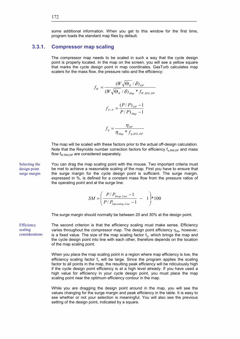
172
some additional information. When you get to this window for the first time, program loads the standard map files by default.
3.3.1. Compressor map scaling
The compressor map needs to be scaled in such a way that the cycle design point is properly located. In the map on the screen, you will see a yellow square that marks the cycle design point in map coordinates. GasTurb calculates map scalers for the mass flow, the pressure ratio and the efficiency:
DPRNIWMapR
DPRW fW
Wf
,,*)/()/(
δδ
ΘΘ
=
1)/1)/(
/ −−
=Map
DPPP PP
PPf
DPRNIMap
DP
ff
,,* ηη η
η=
The map will be scaled with these factors prior to the actual off-design calculation. Note that the Reynolds number correction factors for efficiency fη,RNI,DP and mass flow fW,RNI,DP are considered separately.
You can drag the map scaling point with the mouse. Two important criteria must be met to achieve a reasonable scaling of the map. First you have to ensure that the surge margin for the cycle design point is sufficient. The surge margin, expressed in %, is defined for a constant mass flow from the pressure ratios of the operating point and at the surge line:
100*11/
1/
−
−−
=LineOperating
LineSurge
PPPP
SM
The surge margin should normally be between 20 and 30% at the design point.
The second criterion is that the efficiency scaling must make sense. Efficiency varies throughout the compressor map. The design point efficiency ηdp, however, is a fixed value. The size of the map scaling factor fη, which brings the map and the cycle design point into line with each other, therefore depends on the location of the map scaling point.
When you place the map scaling point in a region where map efficiency is low, the efficiency scaling factor fη will be large. Since the program applies the scaling factor to all points in the map, the resulting peak efficiency will be ridiculously high if the cycle design point efficiency is at a high level already. If you have used a high value for efficiency in your cycle design point, you must place the map scaling point near the optimum efficiency contour in the map.
While you are dragging the design point around in the map, you will see the values changing for the surge margin and peak efficiency in the table. It is easy to see whether or not your selection is meaningful. You will also see the previous setting of the design point, indicated by a square.
Selecting the design point surge margin
Efficiency scaling considerations

173
The map scaling point can also be entered via the keyboard directly into the last two columns of the table. This option is the best choice if you want to reproduce a map scaling point selection that you have made earlier.
If you select the standard component maps, then the map scaling point is automatically placed on the map speed line 1.0 with ßHPC = 0.5. This leads to a surge margin of around 25%.
3.3.2. Turbine map scaling
The scaling of the turbine maps is done in a similar way as the scaling of compressor map. There is no surge line in a turbine map and therefore the task is simpler. The only thing to be checked is peak efficiency, which is dependent on both the map scaling point selection and the cycle design point efficiency.
Both the efficiency and the corrected flow of the high-pressure turbine (HPT) remain fairly constant throughout the operating range of the gas generator of a multi-spool engine. This is because in highly loaded turbines, the corrected flow changes very little for a wide range of corrected speeds and pressure ratios. When the corrected flows at the inlet and the exit of a turbine remain constant, the term P45/P4/√(T4/T45) must also be constant because
45
4545
4
44
45
4
4
45
PTW
PTW
TT
PP
=
The temperature ratio T4/T45 and the pressure ratio P45/P5 are connected by the efficiency:
−−=
−γ
γ
η
1
4
45
4
45 11PP
TT
HPT
In the area near to the turbine design point, efficiency normally does not change very much; the efficiency islands in a turbine map are fairly large. Gas generator turbines will therefore operate at constant pressure ratio and constant efficiency as long as the corrected flow of the power turbine (PT) does not change.
Since the corrected speed NL/√T45 in a helicopter engine normally increases toward partload, the map scaling point should be placed at a moderate map speed, and at a pressure ratio which is higher than the pressure ratio for maximum efficiency. A typical PT operating line can be found in the next chapter.
3.3.3. Off-design calculation options
Only a few input data are required for off-design calculations. On the notebook page with the heading Steady State the first group of input data defines the flight
High-pressure turbine
Power turbine

174
conditions in terms of of altitude, ∆TISA, relative humidity and the Mach number. Installation features like the intake pressure ratio, the power offtake from the gas generator spool, and the bleed air offtake begin the second group of data. Next follow the data that specify the iteration. You can either prescribe the mechanical speed ZXN of the gas generator or the burner exit temperature ZT4. The quantity not specified will be an iteration variable. ß-values in component maps are always iteration variables. All values entered for the iteration variables are used as starting values for the iteration algorithm.
Then there is the input for the relative PT speed. After that are the quantities defining the engine inlet flow distortion. For simulating a variable tip clearance you can make the gas generator turbine efficiency dependent on mechanical speed.
On the notebook page named Modifiers you can specify changes in the turbine flow capacities, the nozzle (=exhaust diffusor exit) area and component efficiencies. Turbine flow capacity is just a different name for the corrected flow.
To calculate the design point in the off-design calculation mode select Task|Single Point and then click the Ok button. You will get a similar cycle summary output on your screen as in the case of a design point calculation. On the page Oper. Point specific off-design data will be provided in addition. On further notebook pages the operating points in the component maps are shown.
Now increase the ambient temperature by setting Delta T from ISA to 10 K and run the cycle calculation again. In the component maps you will see two points. The circle is the design point and the yellow square is the operating point for the increased ambient temperature.
Note that the efficiency contours in the map are valid for Reynolds number index equal 1 and ∆η=0. The actual efficiencies will not be in line with the map values if Reynolds number corrections are applied or if efficiency is modified by the input of a value for ∆η.
Now calculate other operating points and try some of the other input options. When you make large changes in the operating condition from one point to the next the iteration may not converge. Try with better estimates for the variables in such a case or calculate a series of points that are not too far apart in terms of gas generator corrected speed.
3.3.4. Limiters
When calculating a single operating point, you can specify either the gas generator speed or the burner exit temperature. A more flexible option for defining specific operating conditions is to use a limiter from the forth page of the off design input notebook. The program can satisfy several limiters simultaneously. The lowest limit will be the active one.
You can, for example, set limits for NH, T45, T5, WF and for the torque at the output shaft. In addition you can define your own limits using Composed Values. This feature can also be used for calculating a partload case with a specified output shaft power. To do this you must switch off all limiters apart from the general limiter and define the last composed value as PWSD.
Running the cycle to a prescribed shaft power

175
3.3.5. Operating line
An operating line is a series of performance points. The first point is either with specified gas generator speed or a point with limiters switched on. All further points will be calculated with decreasing gas generator speeds. The relative speed will decrease in steps of 0.025. The operating line will either be finished after the specified number of points, or when the operating conditions are far beyond the useful range of one of the component maps.
The number of points to be calculated can be selected from the little box to the right of the red upwards arrow. The sequence of the points to be calculated can be changed using the menu option Direction. An operating line with increasing load is completed when either the mechanical gas generator speed is higher than 104% or when a limiter prevents further increases in load.
Run the example and look at the operating line in the compressor. At very low speed the compressor will surge. There are two ways around this problem: You can either place the design point in the map in such a way that more surge margin is available everywhere or you can bleed off some air at low speed. In practice mostly the second option is used because the first option involves losing compressor efficiency at high power.
A handling bleed schedule can be defined and switched on/off using the option Bleed in the off design input window. The bleed valve will be operated automatically. For this example you should use 0.8 as the upper switch-point and 0.7 as the lower switch-point. The maximum amount of handling bleed could be 20% of the compressor inlet flow, for example. Enter the number 0.2 into the schedule to achieve this.
Look at the operating line of the power turbine. The shape you see is typical for a helicopter engine with a constant rotational power turbine speed. It is quite different from the operating line of the low-pressure turbine of a turbofan.
1
1.5
2
2.5
3
3.5
Pres
sure
Rat
io P
45/P
5
.8 1 1.2 1.4 1.6 1.8 2 2.2 2.4 2.6
NL/sqrt(T45) * W45*sqrt(T45)/(P45/Pstd) [Kg/s]
PT
0.6 0.7 0.8 0.9 1 1.1
1.2
0.93
0.92
0.91 0.90
0.88
0.85
0.80
Figure 13: Operating line of the power turbine
Avoiding surge
Operating line in the power turbine map

176
In addition to the component operating lines you can plot any combination of calculated data. You can compare different operating lines and shifts in parameter combinations caused by changes in flight conditions, installation losses, deterioration (efficiency losses) etc.
3.3.6. Flight envelope calculation
This option calculates a series of performance points for different flight speeds and altitudes. Before starting you should set some limiters. For the fuel flow limiter you need to use the General Limiter, and define the Composed Value 20 as WF. With the model data set DEMO_SHT.CYS the following limiter values might be used for an ISA day flight envelope:
Max fuel flow 0.077 kg/s Max torque 110% of design point torque
Max T45 1120 K Max T5 870 K
Max NH/√ΘR,2 105 % of design point value
This combination of limiters gives an interesting picture of which limiter is active throughout the flight envelope (altitude 0-6000m, Mach no 0-0.5)
0
1000
2000
3000
4000
5000
6000
7000
Altit
ude
[m]
0 .1 .2 .3 .4 .5 .6
Mach Number
NH/sqrt(T)T45T5TRQ
Figure 14 Active limiters within the flight envelope

177
3.4. Turbofan engines
3.4.1. Engine design for subsonic aircraft
Subsonic transport aircraft typically use turbofan engines. The flight condition "end of climb" is usually selected as the design point for such engines. This condition is around 35 000 - 40 000ft altitude and flight Mach number 0.8 - 0.85. The engine design point corresponds to the Max Climb rating.
The file DEMO_TF.CYF, which belongs to the Two-Spool Unmixed Flow Turbofan engine configuration, contains data which are representative of a typical business jet engine. The "end of climb" or "begin of cruise" is assumed to be at an altitude of 11000m (=36089ft) and Mach 0.8. The main design parameters of this engine are
Thrust@11km/0.8 3.12 kN SFC 19.19 g/(kN*s) Corrected Flow W2RStd 55.44 kg/s Overall Pressure Ratio P3/P2 17.325 Burner Exit Temperature T4 1450 K Bypass Ratio 6
The overall pressure ratio of the engine is fairly moderate. The reason for choosing such a design could be to meet the stringent weight and cost targets of the engine. Doing a parametric study will show you what you could gain in terms of the specific fuel consumption by increasing the overall pressure ratio.
The basis of a balanced turbofan cycle design is an optimum combination of the bypass ratio and the fan pressure ratio. How to find this optimum combination is discussed in the next chapter. We will now concentrate on the off-design performance calculations.
Scaling the component maps
First we have to correlate the design point with the component maps. You begin by selecting Standard maps from the main off-design menu. In the standard compressor maps the design point is automatically placed at the map speed line marked 1.0 and at ß=0.5. This point corresponds approximately to the compressor design point. The surge margin is 45% for the fan and 24% for the high-pressure compressor.
The operating point in the high-pressure turbine map is placed slightly above the peak efficiency island with the coordinates (NH/√T4)map=1 and ßHPT=0.5.
In the standard low pressure turbine map the automatic procedure sets the design point at coordinates corresponding to (NL/√T45)map=1.1 and the relative pressure ratio (i.e., ßLPT) at 0.5. This point is close to maximum efficiency, leaving some margin for aerodynamic over-speed operating conditions.

178
You may have a more detailed look at the standard map scaling procedure by selecting Special maps in the main off-design menu. The standard maps are loaded as the default. If you click on the button marked LPC, you will see the fan map. The design point set by the standard map scaling procedure is indicated by a yellow square. If you use the mouse to move the point to the speed line 1.0 and you set the surge margin to 30%, you will get 93.7% as peak efficiency in the map. This is 3.7% higher than the design point efficiency.
An increase of 3.7% in efficiency in going from the aerodynamic design speed to partload is quite reasonable. The absolute level of peak efficiency in our example is high. If you think it is unrealistic, then you should modify the design point efficiency.
You should look at the HPC and the LPT maps as well. You will find peak HPC efficiency to be 0.7% higher than at the design point. The LPT peak efficiency will be 0.1% higher than at the design point.
In the compressor maps in particular the design point need not necessarily be placed at an aerodynamic speed of 100%. If you decide on a lower (NL/√T2)map you will get a greater over-speed margin. There is no need for this, however, if the engine design point corresponds to (nearly) maximum aerodynamic speed. At high altitude, the Max Climb rating is a flight condition with low T2 and high thrust. It practically defines the maximum aerodynamic speed requirements for the turbomachines. It is therefore a good choice to use Max Climb at cruise altitude as the design point, along with the standard map scaling option.
Sea level performance
Go back to the main off-design menu and confirm that the Standard map option is selected to make sure that any modifications you may have made to the map scaling will be reversed. We will now calculate the most important off-design point: sea level "hot day" Take Off. Usually a "hot day" is defined as having between ISA+10K and ISA+20K. You enter Altitude=0, Mach Number = 0 and Delta Tamb= 15K, and set the high pressure spool speed ZXNH to 1.07. You can then start the calculation.
In this example we consider a burner exit temperature T4=1542K, 92K higher than at the design point. This is a reasonable number, since the engine only runs at Take Off rating for a short time compared to the time it runs at Max Climb rating.
When the ambient temperature is lower than ISA+15K, the engine can theoretically deliver more thrust. The thermodynamic thrust of an engine is the thrust developed at ISA inlet conditions with the burner exit temperature of a hot day. Since the aircraft does not need this much power, the engine is normally flat rated. This means that the thrust delivered is limited to the level that the engine produces on a hot day. The curve thrust versus ambient temperature is flat for temperatures below ISA+15K. Consequently, the engine will run colder than T4=1542K on all days with a temperature less than 30°C. At higher ambient temperatures thrust decreases sharply because the burner exit temperature remains constant.
Not every day is a hot day with an ambient temperature of 30°C (86°F) or higher. The peak burner exit temperature is therefore seldom used. The difference between the burner exit temperatures at Max Climb and at maximum Take Off in the example above is quite reasonable.
“Max Climb” as cycle design point
Hot day take off

179
Engine rating
Since thrust cannot be measured when the engine is installed on the aircraft, how is the "flat rating" achieved? There are two alternatives: either NL/√T2 or the engine pressure ratio (EPR) P5/P2 can be kept constant while Tamb decreases below ISA+15K. Try both alternatives! Select the corrected fan speed as the limiter and enter the value NL/√Θ2 which you have calculated for Tamb=ISA+15K. Run the cycle at lower ambient temperature, and then observe the thrust; it will be nearly constant.
You cannot enter a limit for the engine pressure ratio directly. First you must define the composed value 20 as P5/P2 and switch on this newly defined limiter. You will see that also in this case the thrust will be nearly independent of the ambient temperature.
Ambient TemperatureISA ISA+15K
„Flat Rating“
Thrust
BurnerExitTemperature
Thermodynamic Thrust
1469K
12.98kN
14.96kN
1542K
Figure 15: Thrust rating
You can also study the problem the other way around. Define the composed value 20 as the net thrust FN. Then check which cycle quantities are independent of the ambient temperature for constant thrust. Engines with FADEC (Full Authority Digital Engine Control) do not require that you use constant values for the rating parameters. A microcomputer can handle very complicated rating schedules. It is quite normal for the rating parameter to be a complex function of the flight Mach number, the altitude and the deviation from the ISA temperature.
Another feature of rating an engine to NL/√T2 or EPR is that deterioration of the component efficiencies caused by dirt, erosion and increased tip clearances will not cause a thrust loss. Fuel flow will automatically increase and thus cover the additional losses. To look at this, you can enter component deficiencies as Delta Efficiency in your off-design calculations.
GasTurb allows you to use not only constant values for the limiters but also schedules. The off design input window has a menu option Schedules for this purpose. For example, you can specify turbine exit temperature T5 as a function
Control schedules

180
of compressor inlet temperature T2, and so achieve a special thrust characteristic over the flight envelope.
3.4.2. Mixed versus unmixed turbofans
Some engines for subsonic transports have a mixer while others do not. There is a lot to be said for both versions. With GasTurb you can study the consequences of mixing the core and the bypass streams.
Unmixed Flow turbofan
Let us start with the unmixed engine. We want to design a low-pressure system for a given core engine. Which is the best combination of bypass ratio and fan pressure ratio? This problem can be solved analytically; see for example ref. [8]. The answer is that specific fuel consumption will be lowest when the ideal jet velocities V18 and V8 are related to the low spool efficiencies according to
LPTFanideal
VV ηη *
8
18 =
Note that this formula implies special definitions for both the jet velocities and the efficiencies. V8,id and V18,id are ideal velocities: they are calculated from a full expansion to ambient pressure.ηFan takes into account the entire bypass stream pressure loss, and ηLPT all the losses downstream of the low-pressure turbine.
18.8
19
19.2
19.4
19.6
19.8
20
Sp. F
uel C
onsu
mpt
ion
[g/(k
N*s)
]
.5 .6 .7 .8 .9 1 1.1 1.2
Ideal Jet Velocity Ratio V18/V8
Design Bypass Ratio = 5 ... 7 Outer Fan Pressure Ratio = 1.7 ... 1.9
1.7
1.75
1.8 1.85 1.9
5 5.25
5.5
5.75
6
6.25
6.5
6.75 7
1%
Figure 16: Bypass ratio and fan pressure ratio optimization
You can easily convince yourself that the above formula - even if applied to efficiencies that do not take bypass or turbine exit losses into account - is fairly

181
good. Do a parametric study, using the file DEMO_TF.CYF, over a range of bypass ratios and fan outer pressure ratios, and look at the resulting graph SFC versus Ideal Jet Velocity Ratio. Note that you must modify the scales to get the figure to look like the one shown here.
Mixed flow turbofan
For the mixed turbofan there is also a rule for selecting the best combination of fan pressure and bypass ratios. At the mixer entry the ratio of the total pressures P16/P6 must be close to unity. Otherwise, there will be high mixing losses which will decrease the thrust gain. Toward partload the pressure ratio P16/P6 increases. It is therefore good to select a value for P16/P6 that is slightly below 1 for the design point.
The optimum fan pressure ratio for a mixed flow engine is generally lower than that for an unmixed engine, provided that both have the same bypass ratio. When you compare engines with the same fan pressure ratio, the mixed flow engine will have a lower bypass ratio and a higher specific thrust FN/W2. The amount of power, which the low-pressure turbine has to supply to drive the fan, will be smaller when both streams are mixed. This usually allows the mixed engine to be designed with one fewer LPT stage than the unmixed turbofan. The weight saved by this turbine stage helps to compensate for the higher weight of the long duct nacelle needed for the mixed flow engine.
There are other arguments for and against mixed flow engines, involving installation drag, fan noise, reverse thrust etc. You can do a fairly realistic thermodynamic cycle optimization with GasTurb, which includes the effects of low-pressure turbine loading on LPT efficiency. For cycle parameter studies of mixed flow turbofans the fan pressure ratio should be iterated in such a way that P16/P6 is somewhere between 0.95 and 1.
3.4.3. Engine design for supersonic aircraft
The design requirements for an engine of a supersonic aircraft are quite different to those for the engine of a subsonic transport aircraft. We will study the problem using the file DEMO_MTF.CYM, which contains data for a low bypass ratio, mixed flow turbofan with reheat and a convergent-divergent nozzle.
There are several conflicting design requirements for such an engine. High specific thrust and low specific fuel consumption for supersonic flight are the most important criteria. We must also consider Take Off performance. Also the specific fuel consumption for subsonic cruise conditions should not be too high.
Fulfilling this latter criterion leads to a high bypass ratio engine, while fulfilling the first criterion mentioned favors a low bypass ratio. The choices you make very much depend on the mission the aircraft has to fulfill.
The example data file provides you with the performance at sea level static (SLS) conditions, which are shown in the following table. Note that the area ratio of the convergent-divergent nozzle A9/A8 is different for dry and reheated operation. In both cases the nozzle pressure ratio is too low for the given area ratio. The nozzle over-expands the flow, as you can see from the negative pressure thrust term. This and other details will appear on the output screen when you run the

182
example. Note that you must adjust the nozzle area ratio when you switch from dry to reheated operation.
Bypass ratio 1 Burner exit temperature T4 1600 K Overall pressure ratio 17.325 Reheated thrust 48.7 kN Nozzle inlet temperature in reheat T7 2000 K Nozzle area ration in reheat (A9/A8)RH 1.35 Dry thrust 29.4 kN Nozzle area ration in dry (A9/A8)dry 1.2
We will now look at supersonic flight conditions. Calculate the design point with reheat switched on first. Then select the off-design calculation option and use the standard component maps together with the Booster Map Type equal to zero. The area ratio A9/A8 of the convergent divergent nozzle in off design depends on the nozzle throat area A8:
2
,8
8
,8
8
8
9
++=
DesignDesign AAc
AAba
AA
Use a=0.8705, b=0.7325 and c=-0.253. Then enter the following data and start the off-design calculation:
Altitude m 11000 Mach Number 2 HPC Spool Speed ZXNH 1.01
After that change the nozzle area on the page “Modifiers” by 10%:
Delta Nozzle Area % 10
The table on the next page contains the most important results for the two cases A8=A8,Design and A8=A8,Design+10% For the nominal nozzle area, the mechanical spool speed of the gas generator NH exceeds the sea level value (all design point speeds are defined as 100%), but the aerodynamic speed NH/√Θ25,R decreases to 91.9%. The aerodynamic speed of the fan NL/√Θ2,R drops to an even greater extent. This explains the overall pressure ratio of 10.5, which is quite low compared to the pressure ratio at sea level.
The result clearly shows that the standard map scaling procedure must not be applied to supersonic flight conditions. The standard procedure would place the design point at a corrected speed of 100% in all maps. When you run a sea level static flight case, for example, the operating point in the compressor maps would be found at excessively high aerodynamic spool speeds.
You can, of course, also use the standard component maps when defining your engine design point at supersonic flight conditions. You will then have to set the design point in the component maps to an appropriate map speed value significantly below 100%. This can be done with the option Special maps.
The table contains two columns with numbers. Both apply to the same high- pressure spool speed. A bigger nozzle area will improve performance in this case.

183
Whether an increase in the nozzle area helps depends on the flight condition. To see this, take a look at a subsonic high altitude cruise case, for example.
∆A8=0% ∆A8=+10% Thrust 47.1 kN 50.65 kN Burner exit temperature T4 1689 K 1678 K Bypass ratio 1.21 1.36 Overall pressure ratio 10.5 10.6 Nozzle area ratio A9/A8 1.339 1.385 Nozzle pressure ratio P8/Pamb 12.32 11.56 Low-pressure spool speed NL 89.4 % 92.6 % High-pressure spool speed NH 101 % 101 % Fan aerodynamic speed NL/√Θ2,R 76.8 % 79.6% HPC aerodynamic speed NH/√Θ25,R 91.9% 91.9%
For the calculation of dry performance at 11000m, Mach number 0.8 you need to enter some data in addition to the modified altitude and Mach number. Reset the nozzle area to 100%, switch on the NL/√Θ2,R limiter and set it to 104%. You can now start the calculation.
This specific iteration sometimes fails to converge. What can you do to get a valid solution? Click on the Ok button to restart the calculation, this might lead to convergence. If not, look at the data input screen: you may find an unrealistic number for the bypass ratio, for example. Correct it to BPR=1 to provide a revised estimate for the iteration. This should help. If it does not, then look at the estimates for the other iteration variables and enter reasonable numbers.
22
23
24
25
26
27
28
29
30
Sp. F
uel C
onsu
mpt
ion
[g/(k
N*s)
]
2 4 6 8
Net Thrust [kN]
nominal A8A8 + 10%
Figure 17: SFC loops for two nozzle area settings
After you have a solution that converges, start the calculation of an operating line to get a so-called SFC loop which has the shape of a bucket. Bucket SFC is the lowest value you can find along the curve.

184
Figure 3 shows SFC loops for both nozzle areas. In contrast to the supersonic flight case with reheat switched on, the nozzle area has only a minor effect on the SFC loop at partload. However, the maximum thrust decreases when the nozzle area is increased while in the supersonic case the opposite is true.
3.4.4. Engine families
The most expensive part of an engine is the gas generator respectively the “core", which consists of the high-pressure compressor HPC, the burner and the high-pressure turbine HPT. Engine companies therefore strive to use the same core for several applications. Engines with a common core constitute an "engine family".
GasTurb provides special input options that simplify the design of turbofan engine families. We will use the file DEMO_TF.CYF to study an engine family of unmixed flow turbofans.
The Mass Flow Input page offers three ways to define the engine mass flow. If you select option 1, you can enter the fan inlet flow W2√ΘR2/δ2. This is the mass flow corrected to standard day conditions (ΘR2= T2/288.15 K* R/Rdry air,δ = P2/101.325 kPa). If you select option 2, you can enter the core inlet corrected flow W25√ΘR25/δ25. The fan flow will be calculated using the bypass ratio in this case.
The third option also allows you to specify the core flow. You can use an HPC map during design calculations. On the mass flow input page for option 3, you specify the map coordinates ßHPC and (N√T)Map of the HPC operating point. The flow capacities of the turbines will be calculated in such a way that this operating point is achieved.
Before you can start the cycle calculation using the third option you must load an HPC map and adapt it to a reference cycle. Select HPC Map… from the menu and read the standard HPC map HPC_01.MAP as an example. In the following window you can decide to use the map scaled to specified values or you can use the map as it is. Note however, that the mass flow units must be specified when you want to use the un-scaled map.

185
We will scale the map to the standard day corrected mass flow of 3.7 kg/s, an efficiency value of 0.87 and to the pressure ratio of 7 as shown in the top left table.
The values for HPC mass flow, pressure ratio and efficiency will be read from the map as long as option 3 from the Mass Flow Input page remains selected. For example if you set (N/√T)Map=1.1 you will see that core mass flow and pressure ratio will increase and HPC efficiency will decrease.
The value “relative NH” printed in the right column on the summary page is calculated as √(T25/Tstd*R/Rdry air). You can use a composed value and multiply this value by a constant factor to get a more meaningful number for your specific problem.
By doing the experiment with (N/√T)Map=1.1 you will see that the values of the turbine flow capacities W41Rstd and W45Rstd are not the same as those in the reference cycle. Also the HP turbine pressure ratio is significantly different. Obviously the two cycles with (N/√T)Map=1.0 and (N/√T)Map=1.1 do not have the same gas generator and therefore they are not members of the same engine family.
How can you correct this? You must select an iteration with two variables that are adjusted so that the two turbine flow capacities are the same as in the reference cycle. This will automatically result in the HP turbine pressure ratio remaining practically unchanged. As variables you should use the map auxiliary coordinate ßHPC and the design burner exit temperature.
The iteration will converge on a solution in which the jet velocity ratio V18/V8,id is far from its optimum value; this is highlighted by an arrow pointing to the unfavourable number. You can correct this by introducing a third iteration with ‘Outer Fan Pressure Ratio’ as a variable and V18/V8,id=0.85 as the target.
Now you can do some parametric studies. Leave the gas generator corrected speed at its present value of (N/√T)Map=1 for the moment. Select the design bypass ratio and the inner fan pressure ratio as variables. The latter can take booster stages into account if required.
Do a second parametric study with (N/√T)Map=0.9 to see that a wide range of thrust is available from one core engine. Figures 4 and 5 show SFC over thrust for both parametric studies. You should also plot other properties like burner exit temperature and HP spool speed, for example.
All the points from the first and the second parametric study represent engines with the same gas generator. The compressor of the engines in the second case runs at a lower speed and at a lower burner exit temperature T4. Full use of the core temperature and speed potential is required to get a very high thrust. For medium thrust levels alternatives exist that have similar specific fuel consumption values.
Before selecting a cycle you should consider many factors. Both the fan pressure ratio and the number of booster and low-pressure turbine stages are important. You should use the turbine design options offered by GasTurb for the LPT and

186
study different designs. When you have a task with many design variables and constraints, you should use the optimization capabilities of GasTurb.
18
19
20
21
22
23
24Sp
. Fue
l Con
sum
ptio
n [g
/(kN*
s)]
1 1.5 2 2.5 3 3.5 4
Net Thrust [kN]
Design Bypass Ratio = 5 ... 7 Inner Fan Pressure Ratio = 1.5 ... 3
1.5
1.75
2
2.25 2.5 2.75 3
5 5.5
6 6.5
7
1%
T4_D iterated for W41Rstd=1.037Beta iterated for W45Rstd=2.798ZP13q2 iterated for V18q8id=0.85
Figure 18: Parametric study with (N/√T)Map=1
18
19
20
21
22
23
24
Sp. F
uel C
onsu
mpt
ion
[g/(k
N*s)
]
1 1.5 2 2.5 3 3.5 4
Net Thrust [kN]
Design Bypass Ratio = 5 ... 7 Inner Fan Pressure Ratio = 1.5 ... 3
1.5
1.75
2
2.25
2.5
2.75 3
5 5.5 6 6.5 7
1%T4_D iterated for W41Rstd=1.037Beta iterated for W 45Rstd=2.798ZP13q2 iterated for V18q8id=0.85
Figure 19 Parametric study with (N/√T)Map=0.9

187
3.5. Test analysis and engine monitoring
3.5.1. Turbofan test analysis
When a turbofan engine is on the testbed, many measurements are taken. From these measurements the component efficiencies and the high-pressure turbine inlet temperature must be found in a test analysis calculation.
The total engine mass flow W2 is derived from pressure measurements in a bellmouth or in a venturi. The total inlet and exit temperatures and pressures for the compressors are measured. Compressor pressure ratios and efficiencies can be easily calculated.
One part of the total mass flow goes into the core engine, while the other part goes into the bypass duct. It is not possible to measure the core or bypass mass flow directly. Indirect methods must be used to find the flow split.
Make an estimate for the bypass ratio first. This will yield the high-pressure compressor inlet flow W25. Let us assume that we know the amount of bleed and cooling air as a percentage of W25. The air mass flow W3 enters the burner. Now the burner exit temperature T4 can be calculated using the measured value for the fuel flow. The power required to drive the high-pressure compressor can be derived from the compressor mass flow and the measured total temperatures T25 and T3. The temperature T45 at the exit of the high-pressure turbine may then be calculated. The low-pressure turbine exit temperature T5 can be determined on the basis of the power balance between the turbine and the compressors it drives.
For the analysis of the turbine efficiencies the pressures P45 and P5 need to be measured. The turbine inlet pressure P4 is derived from the measured value of the compressor exit pressure P3 using the standard burner theory. The power delivered by the turbines can be calculated from the measurements around the compressors and the core flow.
Now the bypass ratio must be iterated in such a way that the calculated temperature T5 matches the measured value for T5, for example. This method of core flow analysis is called a Heat Balance.
There are, however, several ways to make a core flow analysis. The so-called HPT Capacity method is often used, it is based on a known value for W4√T4/P4. Similarly one can use the LPT capacity W45√T45/P45 to find the core flow.
GasTurb offers Test Analysis for many engine configurations as a special data input option for a cycle design point calculation. For a mixed flow turbofan engine, for example, test analysis can be performed with the following input data:
• Measured Fan Exit Temperature T13 • Measured Fan Exit Pressure P13 • Measured Booster Exit Temperature T21 • Measured Booster Exit Pressure P21 • Measured HPC Exit Temperature T3 • Measured HPC Exit Pressure P3 • Burner Fuel Flow WF • Measured HPT Exit Pressure P44 • Measured LPT Exit Pressure P5
Estimate bypass ratio
Heat balance
Turbine capacity

188
Do not forget to adjust the engine inlet conditions T2 and P2 to the measured values before starting a test analysis calculation.
From the measured data the compressor pressure ratios and the efficiencies will be calculated. Furthermore, the burner exit temperature T4 and the turbine exit temperatures T45 and T5, as well as the turbine efficiencies will be found.
For the core flow analysis define an iteration of bypass ratio to achieve that T5 = T5,measured or that W4√T4/P4= (W4√T4/P4)measured.
3.5.2. Test analysis accuracy
Every measurement has a certain tolerance, so the quantities that are derived from the direct measurements are not exact. This is especially true of the efficiencies of fan and low-pressure turbines of high bypass engines.
GasTurb offers the Monte Carlo method for examining the problem. Take as an example the file DEMO_GTF.CYG and modify the following data:
Altitude from 12000 to 0 Mach number from 0.8 to 0 Bypass Ratio from 8 to 7
Burner Exit Temperature from 1600 to 1830
Switch off LPC Design and HPC Design and then calculate a cycle for sea level static conditions. Print the summary page because we will use this reference cycle output and enter the data from it as ‘measured’ values for the Test Analysis calculation option.
When you have entered all the necessary data for the test analysis option you should do a check calculation. The result should give you values very similar to those of the data you printed earlier. The reason for the very small differences is that the numbers in the printout are rounded.
As an example for a core flow test analysis we select the HP turbine capacity method. We will iterate the bypass ratio in such a way that the turbine flow function value W41Rstd remains constant and equal to the value from our reference printout. Change the bypass ratio for a test to 6 now and try the iteration. When set up correctly, the program will restore the bypass ratio to 7 again.
Go back to the program opening screen and select Monte Carlo from the task list. Do not switch off the iteration. In the Monte Carlo input window you can select quantities which have been measured with a random error. Select in addition to ∆tamb all input quantities for the test analysis option. We assume now for sake of simplicity that all of the temperatures are measured with a standard deviation of 0.1K. This means that 95% of all measurements are within the range ±0.2K around the mean value.
For the pressure measurements, enter a standard deviation equal to 0.5% and use for the fuel flow 0.2% of the reference value. Note that you need to calculate the value of the standard deviation in units of kPa respectively kg/s before you enter it into the table.

189
Figure 20: Input for the Monte Carlo study
Before you click the Ok button you can select a quantity to be shown on the screen while the Monte Carlo simulation is running. Select one you expect to change during the calculation, such as (in our example) the low pressure turbine efficiency.
In a Monte Carlo simulation the specified input parameters will be randomly disturbed with a normal distribution with the specified standard deviation. All randomly generated parameters are independent of each other. When you restart the calculation you will get a new result for the same input because the random numbers are not repeated.
GasTurb can store up to 900 cycle results from a Monte Carlo simulation in a file. From this file you can read selected data, evaluate their statistical properties and plot bar charts. However, you can run the Monte Carlo simulation for many more cycles and observe the quantity that you have selected, before pressing the Start button. When you click the Stop button then the mean value as well as the standard deviation for all of the simulated cycles will be shown on the screen.
The calculation you have started will take some time because an iteration is required for each cycle.
From this exercise we get many statistical distributions. Some interesting data describing the test analysis accuracy are:
mean 2 σ Outer Fan Efficiency 0.879 ±0.017 LPT Efficiency 0.900 ±0.006 Stator Outlet Temperature 1785 K ±10 K

190
Certainly the accuracy for the Outer Fan Efficiency is not acceptable. Every effort must be made to measure the fan inlet and exit temperatures as precisely as possible.
3.5.3. Comparing a performance simulation with test data
When you have got data from another cycle program, from measurements or from literature you are certainly interested how these data compare to simulation results from GasTurb. You can read those data from file and show them together with the GasTurb results for an operating line.
Using the Test Analysis option makes the adjustments of the GasTurb input data for a single cycle very easy. On the compressor side all temperatures and pressures are given and that defines implicitly efficiency and pressure ratio for each compressor. On the turbine side the pressures are also input to GasTurb. The only unknowns are the air system properties and the mechanical efficiencies.
Adjust the air system properties in such a way that the calculated temperatures in the hot section of the engine line up with the given values. This can be done with parametric studies, possibly combined with iterations. You can also use an optimization in which the air system properties are the optimization variables and the figure of merit is the sum of all (Tcalculated -Tgiven)² from the hot section of the engine.
When you have found the best match to the given data, then mark the checkbox Overwrite P/P, Eff and T4 input and run the calculation once more. This will modify your compressor pressure ratio, T4 and efficiency input data in such a way, that you get with the Test Analysis switch in off position the same result as with the on position.
You can compare off-design data you have got from elsewhere with the calculated data from your model. Select File|Read Comparative Figures in the operating line calculation window to read the given data from a file before calculating an operating line, and then plot them together with the calculated data from a single operating line.
The file with the given data is an ASCII file, which can be produced with any editor. The default file name extension is tst (file name example: PassOff.tst). The file format is described in the GasTurb Help file under the heading “Compare Data with GasTurb Results”.
3.5.4. Test analyis by synthesis
The test analysis method described above makes no use of information that is available from component rig tests, for example. It will give no information about the reason, why a component behaves badly. A low efficiency for the fan may be either the result of operating the fan at aerodynamic over-speed or the result of a poor blade design. To improve the analysis quality in this respect is the aim of Analysis by Synthesis (AnSyn). This method is also known as model based engine monitoring.
When doing analysis by synthesis a model of the engine is automatically matched to the test data. This is done with scaling factors to the component models, which
Adjusting a GasTurb model
Comparing data for an operating line

191
close the gap between the measured efficiency and the model. An efficiency scaling factor greater than one indicates, that the component performs better than predicted, for example.
The AnSyn factor for efficiency is defined as
el
measuredEAnSynf
mod, η
η=
Similarly, the flow capacity AnSyn factor is defined as
el
R
measured
R
CAnSynW
W
f
mod
,*
*
Θ
Θ
=
δ
δ
A factor of 1.0 means perfect agreement between the model and the measurement. For each compressor respectively turbine there is a flow capacity and an efficiency factor defined.
Similarly other AnSyn factors can be derived from the difference between measured and calculated thrust of a jet engine, for example. It depends on the engine configuration which AnSyn factors are used during test analysis.
Finding compressor map scaling factors
Let us explain the procedure for the example of a compressor. The model of the compressor is a calculated or measured map which contains pressure ratio over corrected flow for many values of corrected spool speed N/sqrt(T). During the test analysis we obtain from the measurements the pressure ratio, the corrected mass flow, the efficiency and the corrected spool speed. Normally we will find, that the point in the map defined by the measured pressure ratio and the measured corrected flow (marked in the figure by the open circle) will not be on the line for N/sqrt(T) in the original map.
We can shift the line marked N/sqrt(T)map in such a way, that it passes through the open circle. This is done along a scaling line that connects the open circle with the solid circle. The mass flow and the pressure ratio scaling factors can describe the distance between the two circles. The efficiency scaling factor compares the analyzed efficiency with the value read from the map at the solid point.
There are many ways to select a scaling line. A good choice is scaling along a line with H/N²=constant. In GasTurb the auxiliary map coordinate ß is used as a scaling line because this makes the calculations simple and at the same time approximates the scaling along a line with H/N²=constant very well.
Compressor performance monitoring

192
Figure 21: Compressor analysis by synthesis
Along the scaling line there is a correlation between the mass flow scaling factor and the pressure ratio scaling factor. Therefore it is sufficient to use the mass flow scaling factor alone. The pressure ratio scaling factor is calculated from the mass flow scaling factor from the rule ß=constant.
Data input for a single scan
Test analysis by synthesis is an option in the off-design input window, select it from the menu as Task|Analysis by Synthesis. It is a good idea to set all modifiers to zero before actually starting test analysis. When you use the file DEMO_MTF.CYM (Two Spool Mixed Flow Turbofan), you will get the following data input example on your screen:
The scan identification number is an arbitrary number, which serves for documentation purposes. Running the model for 500m altitude, -20°K deviation from ISA ambient temperature and ∆ηHPC=0.01 has produced the other data in the table.
To the right of the test data table you can select between four core flow analysis methods. Select one of them and click the Ok button to start the test analysis calculation. When completed, the notebook page Deviations from Model will show up, see next figure. Select View|Detailed Output to get the full diagnosis output for this scan.
The deviations from the model are shown as factors and temperature differences. In this example only the HP compressor efficiency factor deviates from the nominal value, the program identifies correctly the abnormality in the data.

193
Figure 22: Single point test data input for a mixed flow turbofan
Figure 23: Test analysis result
Now go back to the off-design input window and change the model by entering “1” for Delta HPC Efficiency [%] on the Modifiers page. Rerun test analysis for the example data and you will find that now no deviation from the model is diagnosed.

194
Change back Delta HPC Efficiency [%] to 0 and run again the test analysis. The HPC efficiency factor is calculated as 1.01183, which equals 0.8558/0.8458. The efficiency difference is exactly 1%.
Clicking on the button with the two-sided arrow (or selecting Task|Effects) will show the effects of small changes in the measurements on the results for the AnSyn factors. The step sizes are equal to the measurement tolerances given with the measured data.
You can customize your simulation model, which is normally representing an average new engine, and adapt the turbine flow capacities and the internal air system to the specific test vehicle where your measurements come from. On the second page of the notebook you can enter relative turbine capacities, there the nominal value is 100%. The numbers you enter here will have an impact on the result especially when you use a turbine capacity analysis method. Similarly the numbers on the “Air System” page can be used to customize the model.
Sensor checking
The interpretation of measurements poses always the question: is the sensor inaccurate or a component of the gas turbine degraded? The option Check Sensors tries to answer this question with the help of AnSyn as described below:
It is assumed that only one sensor is inaccurate. At first the sum q0 of the absolute deviations of all AnSyn factors from 1 is calculated:
∑ −= 10 AnSynfq
Next for each of the sensors an optimization is done in which the optimization variable is the sensor reading and the figure of merit is:
∑ −= 1Ansyni ffom
Thus for sensor i a theoretical reading ri is found together with the figure of merit fomi.
When all optimizations are finished, then the differences di = q0 - fomi are checked. The sensor j for which dj has the highest value is potentially indicating the wrong value. When the measured value deviates more than the measurement tolerance from the theoretical reading rj then a sensor error is declared.
Note that the magnitude of the AnSyn factors depends on the flow analysis method. Therefore the result of a sensor check depends also on the mass flow analysis method.
Do an experiment with the example data: set T3 to 690K and select Task|Sensor Checking
The program will find that T3 is potentially incorrect and supposes as reading the value 701.8K, which is correct. Note however, that this method of sensor checking will not in all cases give right answers. For example, when compressor capacity has changed, then a spool speed measurement problem might be diagnosed.

195
ISA correction
During a normal engine test at a standard sea level testbed, for example, both the inlet pressure and the inlet temperature will deviate from ISA sea level standard conditions (T = 288.15K, P = 101.325kPa). The test results must be corrected to these engine inlet conditions to make the data comparable.
The correction of the measured values to ISA standard day (respectively nominal) conditions is very easy when the AnSyn approach is used. The scaling factors found from the analysis of the scan are applied to the model and then the model is run at the same corrected low-pressure spool speed and the ISA engine inlet conditions.
The operating conditions of the turbofan engine will not be exactly the same for both the test and the calculation of the ISA corrected performance. This can be seen eventually from the calculated value for the corrected high-pressure spool speed which will be only very near to (but not exactly the same as) the measured value. The reason for that are the many small effects which do not allow strict Mach number similarity between the tested and the ISA corrected cases like
• gearbox drag • fuel, oil and hydraulic pump power • changes in gas properties • Reynolds number effects • thermal expansion of rotors, blades and casings
Schedule correction
The measured test data from a single scan can be corrected to ISA conditions. However, also the rated performance has to be derived from engine performance tests. With the conventional test analysis this requires a set of scans which include the power range of interest. Then a curve fit is applied to the ISA corrected data and the resulting curve is read at the exact value of the rating parameter. This might be a rated temperature, a spool speed or an engine pressure ratio, for example.
With the AnSyn approach one can easily evaluate the rated performance by just running the calibrated model (which is either based on a single or on multiple scans) at rated power. The rated power is defined by a limiter or by a control schedule like T5=f(T2), for example. Therefore the correction to rated power is called schedule correction.
Data input for multiple scans
Test data for multiple points can be read from a file with the extension .MEA. The file format is as follows

196
ScanId humid! W2! XN_LP_A! XN_HP_A! T2! P2! … Tolerances 0 10 0.5 0.03 0.03 0.2 0.3 … Measured Data 10 60 182.5 100 100.5 288 99.02 … 11 60 180.2 99.5 99.8 287.5 99.1 … 12 60 172.5 99.1 99.5 287.8 99.05 … 13 60 168.2 98.5 99.3 287.9 99.07 … 14 60 164.1 97.8 98.9 287.4 99.04 … … … … … … … … …
The first line must begin with ScanId followed by the short names of all measured data that are defined for the selected engine configuration. The next two lines are optional. They give the tolerances for the measurements in percent of the actual value.
The key words Measured Data precede the lines with the measured data. The number of scans is limited to 30. When more than 30 scans are in the file, then only the first 30 scans will be read.
You can create an example file with measured data for AnSyn by selecting Help|Create Data File Example from the menu in the Analysis by Synthesis window.
The data in this example file will be based on the measured data shown on the Test Data page. The numbers will follow a normal distribution with the standard deviation equal to the measurement tolerance.
Analysis of multiple scans
After you have loaded a series of scans you can use the spin edit box marked “Scan Sequence No.” to scroll through the scans and analyze scan after scan. However, you can also run the analysis automatically for all scans by selecting View|AnSyn Graphs.
This will open a window in which you can select, for example, a graph in which the HPC Efficiency Factor is plotted over Scan Identification No.. In this graph you will see, that the HPC Efficiency Factor is scattered around 1.12. The reason for this result is, that the test data set was created after loading the file DEMO_MTF.CYM (which contains test data produced with ∆ηHPC=0.01) with the menu option Help|Create Data File Example.
You can also compare the model with the test data by selecting View|Model Comparison. Then the model will be run automatically in such a way, that T2, P2, Pamb and the gas generator spool speed are as measured. All other measured data will deviate more or less from the model because the model is never perfect.
It is a good idea to use Composed Values when comparing measured data with a model. Plotting the ratio P25/P25! over W25Rstd is much more meaningful than plotting P25 over P25!, for example.
There is a further option to compare the measured data with the model. After you have loaded many scans, you can close the Test Analysis window and run a single operating line with engine inlet conditions in terms of T2, P2 and Pamb that are typical for the test. The test data are automatically stored as Comparative
Comparing test data with a model
A second option for comparing test data with a model

197
Figures as you can see from the menu option File|Show Comparative Figures in the operating line window:
Figure 24: Compare test data with the results from an operating line calculation
When you do not get test data plotted with the operating line then check the scales of the graph: the test points might be outside of the x- respectively y-axis ranges.
Output of analysis results to file
You can direct the output of the calculation to a file, which you can later read with other programs, for example. A pure ASCII file will be created with the short names as headline. At first you have to define the quantities you want to store in the file by selecting Output|Define from the menu.
Select from both the input and output quantities. By clicking on the button INPUT respectively OUTPUT you can toggle between the two lists. You can also add groups of data to the list by selecting Quantities|AnSyn Input and Quantities|AnSyn Output from the menu.
Save your output parameter selection with the command File|Save Selection. This will write just the headline with the short names of the selected properties to the file. Opening a file with File|Read Selection will evaluate the file header and fill the output list box.
Besides defining the file content you have to specify a file name. You need not specify an extension for the filename because it will be selected automatically. After closing the output selection window the file is open for output of the analysis results from a single scan or from all scans. After writing to the file you can edit it and add comments, for example. You can write the test data as measured, or after ISA or schedule correction to file.

198
Engine monitoring
For engine performance monitoring take measurements at stabilized operating conditions, analyze the scans and monitor the changes in engine health parameters. The AnSyn factors are especially well suited as health parameters because they describe the difference between a nominal engine and the engine being monitored.
For long term monitoring you should read groups of scans into GasTurb, analyze them with one or several core flow analysis methods and store the results in a file. You can store ISA corrected data, schedule corrected data or just the measured values together with the AnSyn factors, for example.
Read the GasTurb output file into a spreadsheet and look for trends in the data. You may observe that the flow capacity of the first compressor decreases slightly, and so does the efficiency AnSyn factor. This would give you a hint that the compressor should be washed to recover some of the performance, for example.

199
3.6. Optimization
In a parametric study with only two variables it is easy to find an optimum solution. If there are three variables the situation is not so clear. With more than three variables the picture may get obscure. In complex studies the true optimum may never be found. However, mathematical optimization routines make it possible to handle many variables.
3.6.1. The use of optimization
What is "optimization" in a mathematical sense? It requires a mathematical model of reality. A complex engine model, for example, provides many outputs such as thrust, fuel consumption, weight, noise, manufacturing cost etc., for any meaningful combination of input variables.
One quantity is selected as a figure of merit: The mathematical model is then driven to an extreme value of the figure of merit by the optimization algorithm. You can, for example, ask for the engine with the lowest weight.
The figure of merit alone does not fully describe the problem. Normally there are constraints for both the variables and the results. For an engine of a subsonic transport aircraft the optimization task could be: Minimize specific fuel consumption (figure of merit = SFC) with the following variables:
min max Bypass ratio 6 BPR 12 Outer fan pressure ratio 1.5 P13/P2 1.8 IPC pressure ratio 1.5 P24/P2 6 HPC pressure ratio 6 P3/P25 12 Burner exit temperature 1400K T4 1800K
The constraints are:
min max HPC exit temperature T3 840K HPT exit temperature T45 1250K Thrust 30 kN FN HPT pressure ratio P4/P45 3.2
It is not obvious how the variables affect the constraints. In many cases the relation between optimization variables and the constraints is very complex. It is impossible to see instantly whether a specific set of variables fulfils the constraints.
Let us be more general now: The mathematical model of the engine is a function which provides exactly one value for the figure of merit Z and several values Cj for the constraints, for a set of optimization variables Vi.
There are only a few rules for setting up a mathematical model. The figure of merit and the values for the constraints must depend on the optimization variables directly. If a certain combination of variables results in an invalid figure of merit, the model must reply with an error message. Then it must give the control back to the optimization algorithm again.
Figure of merit
Variables and constraints
200
We are looking for an algorithm to find the optimum set of variables. This set must have the highest figure of merit possible without violating any constraint. A minimization task can, by the way, be easily converted into a maximization task by multiplying the figure of merit by -1.
Here is a good analogy for the task: A mountaineer shall climb the highest peak in a certain region. He has no map, and the weather is foggy. His only tool is an altimeter. What will he do? He will certainly check his surroundings first and then go in the direction of the steepest ascent. In the end he will come to the top of a mountain. This is a place where each step leads downwards.
The steepest ascent may, however, lead toward a border of the region. Then our mountaineer will walk along the border until he reaches the place where each step leads downwards, or out of the allowed region. Is that the end of the story? Not necessarily. There might be several summits within the region. Our mountaineer may have found the highest peak by chance, but he cannot be sure of that. He has to check other parts of the region. In mathematical terms there might be "local" optimums in addition to the "global" optimum.
Up until now we have not spoken of constraints. These are like fences. A part of the region is forbidden to our mountaineer. His task is made more difficult because on his way to the summit he may have to walk downwards for a while to avoid a forbidden region. The fences, or constraints, often exclude a summit (where each step leads downwards) as an acceptable solution. They create local optima that would not exist without fences. Constraints make the task of optimization difficult.
Gradient strategy
Let us turn to the mathematical algorithm now. The mountaineer who first makes test steps in several directions uses the gradient strategy as a search method. He takes test steps in order to find the partial derivatives δZ/δVi. For each optimization variable he must make one test step before he can start his way in the right direction.
When the mountaineer takes the first step uphill, the local gradients change. He must take new test steps to find the new direction of steepest ascent. Taking test steps takes time, however, and it is therefore better for the mountaineer to continue in the same direction as long as the altitude increases. When he reaches a fence (i.e. violates a constraint), the mountaineer stops climbing. Only then will he make new test steps (seek gradients). The process will eventually take him along a fence.
GasTurb offers two optimization algorithms. The first is derived from ref. [9]. The principle is the following (see figure). We begin at the point marked "Start 1", looking for the direction of the steepest gradient ("Direction 1"). Following this direction we walk to the highest point. Then we change direction by 90° (orthogonal). We can do this without evaluating the local gradient. Then once again we look for the highest point. To define the third direction we use the knowledge of the first two directions. We connect the point "Start 1" with the optimum point found along "Direction 2". We follow this direction as long as altitude increases.
This procedure can be reapplied until the search steps or the changes in the figure of merit become very small. There is a maximum limit for the number of
Local and global optima

201
optimization steps. In the example shown in the figure the optimum is found along search direction 7.
Start 1
Start 2
Direction 1
Dir 2
Direction 3Dir 4
A
Figure 25: Optimization with a gradient strategy
Up until now we have only dealt with optimization without constraints. In the figure there is a shaded zone which suggests a forbidden region. If we use the strategy just described the search for the optimum will end at point "A" along "Direction 2". We cannot find the global optimum if we begin at "Start 1". If we begin at "Start 2", however, we will reach the top of the hill very quickly.
Do not underestimate the danger of finding only a local optimum, particularly in cases involving several constraints. You should repeat the optimization from several starting points. GasTurb offers the option Restart for this purpose. The program uses random numbers as the optimization variables and checks, which is the worst combination. The constraints must be fulfilled for a new starting point. When you have found the same optimal solution from several starting points, you can be quite sure that you have found the global optimum.
Adaptive random search
Alternatively, you can try the second optimization strategy offered by GasTurb, which is based on ref. [10]. In an adaptive random search, random numbers concentrated around the best solution found previously are used as the optimization variables. The algorithm is
( ) vk
R
iii k
RVV 12* −Θ+=
with

202
Vi new value of optimisation variable Vi
* value of Vi producing the best figure of merit Ri search region for variable Vi kR range reduction coefficient (positive integer) kv distribution coefficient (positive odd integer) θ random number between zero and one
To start an adaptive random search you should have a variable combination that fulfils all of the constraints. At the start of the search kR is 10 and kv is 1. In one search run GasTurb tries 40 times the number of Optimization Variables random engine cycles. When all cycles have been calculated, then kR will be duplicated and kv will be increased by 2. The search region will get smaller. Another 40 times the number of Optimization Variables cycles will be calculated, and then kR will be duplicated again and kv will be further increased by 2. This procedure will be repeated until all cycles for kR=80 have been tried. Cycles that do not fulfil the constraints will be ignored.
Each time the adaptive random search stops you can also switch over to the alternate search strategy. Along with the Restart option this constitutes a very flexible tool for mathematical optimization.
3.6.2. A simple example
An optimization task involving five variables and four constraints was presented in the introduction to the previous chapter. You can solve this task using GasTurb. Select a "geared turbofan" as engine and use the data file DEMO_GTF.CYG.
The optimum solution shows a figure of merit (=SFC) of 16.45 and the following variables:
Bypass ratio 8.4 Outer fan pressure ratio 1.65 IPC pressure ratio 5.99 HPC pressure ratio 6.22 Burner exit temperature 1644K
All constraints are fulfilled with this cycle. Thrust is exactly 30kN. The HPT exit (=LPT inlet) temperature is at its limit of 1220 K and the HPT pressure ratio is 3.2. However, the compressor exit temperature, which is 824K doesn't reach its maximum value.
You will not get this solution on the first trial, but will probably need to restart the optimization several times. When you have come reasonably close to the solution, you should also look at the “landscape” in the vicinity of the optimum. Is there a distinct optimum or is the region around the optimum fairly flat? Would it be better to deviate slightly from the optimum to get a benefit that is not described by the figure of merit?
Sometimes you will get a surprising result for the optimization variables. If you have obtained the optimum according to the mathematical model, but the result looks unreasonable, the figure of merit or a constraint may have been defined awkwardly. Alternatively, the mathematical model may not be representative. Often you can see immediately which part of reality has not been described correctly. In such cases optimization gives you a hint as to how to improve your

203
model. Also the result might not be as unreasonable as it looks at first sight. Optimization may give you new ideas - and that can never do any harm.
3.6.3. Cycle selection for a derivative turbofan
A very common design task is adapting an existing engine for a new application. In this case there are more constraints than in the design of a brand new engine. In this chapter first the basic engine, and then the design variables, the constraints and the figure of merit for the numerical optimization of a derivative engine, will be described.
Description of the basic engine
Let us assume that we can start from an existing unmixed flow turbofan engine for a business jet. This type of engine has a rather low overall pressure ratio and a moderate burner exit temperature, compared to the big turbofan engines used on commercial airliners. The main cycle parameters are shown in the table below.
Flight condition 11km/Mach 0.8, Max Climb, installed
Thrust 3.63kN SFC 19.7 g/(kN*s) Bypass ratio 4.5 Burner exit temperature 1350K Overall pressure ratio 17.82 Core pressure ratio 12 ISA corrected mass flow 60 kg/s
Design variables, constraints and figure of merit
Besides the pressure ratios of the new booster and of the fan, the bypass ratio and the burner exit temperature are among the design variables of the growth engine. A new low-pressure turbine will be required, but the gas generator will remain unchanged.
The core compressor of the new engine must not necessarily be operated at the same operating point as in the basic engine. In fact doing that might be impossible, because it would require an increase in the mechanical spool speed beyond the limits of the original design. Thus we obtain the core compressor mass flow and pressure ratio as two additional design variables for the derivative engine.
It is standard practice to read a compressor map using given corrected speed and a value for an auxiliary coordinate (here called beta) rather than using given mass flow and pressure ratio; see for example ref. 4. In the list of the design variables we get, instead of the compressor mass flow and its pressure ratio, the two equivalent variables corrected speed and map coordinate beta.
Altogether there are six design variables for the derivative engine.
Design variables

204
There are several constraints that must be observed in designing the new engine. For the common core with the basic engine, both high-pressure turbines must have practically the same flow capacity. We also want the Mach number at the core exit to be nearly the same for both engines, and consequently, the flow capacity of the low-pressure turbine must be very similar in both engines. Hence there will be practically no difference in the high-pressure turbine pressure ratios of the engines.
An additional constraint is that the low pressure turbine inlet temperature T45 must be below say, 1150K, which allows us to design an un-cooled low pressure turbine from inexpensive materials.
The core compressor is responsible for several constraints in the design. There might be a temperature limit if the last stage is made from titanium, for example. Also, a mechanical speed limit may exist. There may be constraints associated with meeting the minimum surge margin requirements. Another possible constraint, which will limit the fan diameter of the growth engine, is associated with the nacelle in which the engine has to be installed.
In our example the task is to increase the Max Climb thrust by 23% to 4.5 kN. Engine designs with less thrust than required will not be acceptable; therefore the thrust is a design constraint for the growth engine. In summary, the design constraints for the derivative engine are:
HP turbine flow capacity Reference value ± 5% LP turbine flow capacity Reference value ± 5% LP turbine inlet temperature T45 < 1150K HPC exit temperature T3 < 750 K Core spool speed NH < Reference value + 5% Fan tip diameter < 0.75 m Max Climb thrust > 4.5 kN
The specific fuel consumption (SFC) for Max Climb rating is the figure of merit which is to be minimized. A low fuel consumption for cruise will result automatically.
Mathematical model of the engine
A mathematical model of the growth engine requires a combination of design and off-design calculations. The components of the low-pressure spool will be newly designed, while the core components will be operated at some off-design condition with respect to the design point of the basic engine.
We select the Max Climb rating at altitude as the cycle design point for the growth engine. For this flight condition the optimum values of the design variables will be found.
The mathematical model of the engine must take into account that the design point efficiencies of the fan, the booster, and the low-pressure turbine will change with the aerodynamic loading. For axial compressors we can use an appropriate correlation which has been published by Glassman (ref. 11), and for the low-pressure turbine we can use a simplified version of the preliminary turbine design routine from Warner (ref. 3).
Constraints
Figure of merit

205
The efficiency and the surge margin of the core compressor will be read from the map using the values for the design variables core compressor corrected speed and map coordinate beta.
Note that the temperature limits for T3 and T45 in the list of constraints are not applicable to the Max Climb rating, but to the flight case in which temperatures are highest. Hence the numerical model of the engine must be capable of simulating both the Max Climb flight case at altitude (as a cycle design point) and the Take Off rating for the hot day (ISA+15K) at sea level, Mach 0.2 (as an off-design condition). Note that during Take Off the engine runs with a 7% higher mechanical high-pressure spool speed than at Max Climb in this example.
When constraints from an off-design point must be taken into account, then go for off-design, select Task|Mission and define a mission with one single point before initiating the optimization. Then you have for each of the seven constraints the choice, whether it applies to the design point or to the off-design point.
Optimizing the growth engine
Before performing the numerical optimization algorithm, we need to define a range for the design variables. On one hand this range should be as narrow as possible so that the search for the optimum will take less effort. However, if the range is too narrow, the true optimum might be excluded from the search unintentionally.
Another reason for setting the range of a design variable can be that either the lower or the upper limit represents a true limit for the engine design. In our example this is the case for the pressure ratio of the single stage fan, which is introduced with an upper limit of 1.9. In the table the ranges for all six design variables are given.
The numerical optimization algorithm requires that a set of design variables, which fulfills all constraints, be known before the calculation can commence. The cycle of the basic engine is within the ranges of all design variables; however, it does not fulfill the minimum thrust constraint.
How can we get a valid cycle to start with? One possible approach is to do a rough parametric study, which aims to find only a feasible solution, but not the best solution for the problem. However, such a parametric study would take more effort than necessary. For the moment, we can redefine the figure of merit and do a slave optimization to maximize the Max Climb thrust. The minimum thrust constraint is dropped for this preliminary exercise, which assumes that the basic engine cycle is valid as a starting point.
While the slave optimization is running, we can observe the progress on the computer screen. As soon as a cycle is found which has more Max Climb thrust than required (and fulfills all constraints) we can stop. We redefine the figure of merit as specific fuel consumption and introduce the minimum thrust constraint. Then we can begin the final optimization.
The figure shows the optimization window of GasTurb for the example given here, with six horizontal gauges for the design variables on the left and seven gauges for the constraints in the upper right part. The gauges are continuously updated while the optimization is running. In the lower part of the screen the figure of merit is represented both graphically, with a dot for every valid solution, and numerically.
Ranges for the design variables
Starting point
Graphical user interface
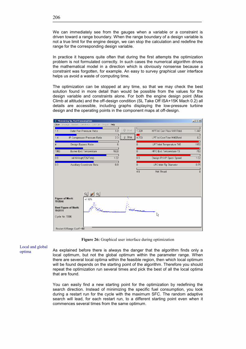
206
We can immediately see from the gauges when a variable or a constraint is driven toward a range boundary. When the range boundary of a design variable is not a true limit for the engine design, we can stop the calculation and redefine the range for the corresponding design variable.
In practice it happens quite often that during the first attempts the optimization problem is not formulated correctly. In such cases the numerical algorithm drives the mathematical model in a direction which is obviously nonsense because a constraint was forgotten, for example. An easy to survey graphical user interface helps us avoid a waste of computing time.
The optimization can be stopped at any time, so that we may check the best solution found in more detail than would be possible from the values for the design variable and constraints alone. For both the engine design point (Max Climb at altitude) and the off-design condition (SL Take Off ISA+15K Mach 0.2) all details are accessible, including graphs displaying the low-pressure turbine design and the operating points in the component maps at off-design.
Figure 26: Graphical user interface during optimization
As explained before there is always the danger that the algorithm finds only a local optimum, but not the global optimum within the parameter range. When there are several local optima within the feasible region, then which local optimum will be found depends on the starting point of the algorithm. Therefore you should repeat the optimization run several times and pick the best of all the local optima that are found.
You can easily find a new starting point for the optimization by redefining the search direction. Instead of minimizing the specific fuel consumption, you look during a restart run for the cycle with the maximum SFC. The random adaptive search will lead, for each restart run, to a different starting point even when it commences several times from the same optimum.
Local and global optima

207
In the figure one can see from the graphics for the figure of merit that a restart has happened twice. This is because the algorithm Endless Random Search restarts automatically after it has homed into an optimum. The best solution found will be stored in memory and can be restored as soon as the calculation is stopped.
Some important data for our growth engine example is summarized and compared to the basic cycle data in the next table.
Basic engine Growth engine Max Climb Hot day
Take off Max Climb Hot day
Take off Thrust [kN] 3.63 12.1 4.5 16.1 SFC 19.7 14.4 19.0 13.5 Bypass ratio 4.5 4.67 5.03 5.15 Fan P13/P2 1.8 1.59 1.69 1.56 Ideal Jet Vel. Ratio 0.78 0.91 0.68 0.77 Booster P24/P2 1.5 1.27 1.82 1.58 HPC P3/P25 12 11.3 12.4 11.7 T4 [K] 1350 1460 1399 1522 HPT flow capacity 1.378 1.39 1.31 1.32 LPT flow capacity 4.95 4.92 4.95 4.95 T3 [K] 611 700 654 750 T45 [K] 976 1060 1005 1097
Discussion of the result
The optimum growth engine is affected by three design constraints: First, it has a fan diameter of 0,75m; i.e., it uses the largest fan allowed in this exercise. Second, the compressor exit temperature is at the limit of 750 K for the hot day Take Off case. Last, the minimum high-pressure turbine flow capacity is found to be the best solution.
All design variables did remain within the predefined range during the optimization. The thrust for Max Climb rating at altitude is 4.5 kN. The specific fuel consumption at altitude is 3.5% better for the growth engine than for the original.
The table also contains a row for the ideal jet velocity ratio. From theoretical considerations we can derive that this ratio should be equal to the product of fan and low-pressure turbine efficiencies when an unmixed flow turbofan is to be optimized for SFC. Note that the numerical optimization algorithm has automatically found a cycle for which the jet velocity ratio is near to its theoretically best value.

208

209
4. Nomenclature
4.1. Station Definition
The station definition used in the program follows the international standard for performance computer programs. This standard has been published by the Society of Automotive Engineers SAE as ARP 755A.
0 ambient 1 aircraft-engine interface 2 first compressor inlet 125 bypass mixer inner inlet 13 outer stream fan exit 16 bypass exit 161 cold side mixer inlet 163 cold side mixing plane 18 bypass nozzle throat 21 inner stream fan exit 225 bypass mixer outer inlet 24 intermediate compressor exit 25 high pressure compressor inlet 3 last compressor exit, cold side heat exchanger inlet 31 burner inlet 35 cold side heat exchanger exit 4 burner exit 41 first turbine stator exit = rotor inlet 42 high pressure turbine exit before addition of cooling air
(three spool engines) 43 high pressure turbine exit before addition of cooling air
(two spool engines) 43 high pressure turbine exit after addition of cooling air
(three spool engines) 44 high pressure turbine exit after addition of cooling air
(two spool engines) 44 intermediate pressure turbine inlet
(three spool engines) 45 low pressure turbine inlet
(two spool engines) 45 intermediate pressure turbine rotor inlet
(three spool engines) 46 intermediate pressure turbine exit before addition of cooling air
(three spool engines) 47 low pressure turbine inlet
(three spool engines) 48 low pressure turbine exit before addition of cooling air 5 low pressure turbine exit after addition of cooling air 6 jet pipe inlet, reheat entry for turbojet, hot side heat exchanger inlet

210
61 hot side mixer inlet 63 hot side mixing plane 64 mixed flow, reheat entry
7 reheat exit, hot side heat exchanger exit 8 nozzle throat 9 nozzle exit (convergent-divergent nozzle only)

211
4.2. Symbols
The symbols for mass flow, pressures and other quantities are also defined in ARP 755C. They are composed of the station name and some leading letters. The following symbols are used in this manual and the program:
A area alt altitude amb ambient ax axial Bld bleed BPR bypass ratio corr corrected C constant value, coefficient C compressor CFG thrust coefficient Cl cooling d diameter dH enthalpy difference dp design point ds design DC pressure distortion coefficient DT temperature distortion coefficient f factor f fuel far fuel-air-ratio F thrust FN net thrust FG gross thrust h enthalpy H high pressure spool HdlBld handling bleed HPC high pressure compressor HPT high pressure turbine i inner I intermediate pressure spool IPC intermediate pressure compressor IPT intermediate pressure turbine L low pressure spool Lk leakage LPC low pressure compressor (fan) LPT low pressure turbine M Mach number N spool speed NGV nozzle guide vane NHR NH√T/( NH√T)dp NLR NL√T/( NL√T)dp o outer P total pressure prop propulsion PSFC power specific fuel consumption PT power turbine PW shaft power R gas constant rel relative RH reheat

212
RNI Reynolds number index s static SD shaft, delivered SFC specific fuel consumption SFR steam-fuel-ratio t (blade) tip t time T total temperature TRQ torque TSFC thrust specific fuel consumption U blade (tip) velocity V velocity VABI variable bypass injector VCE variable cycle engine W mass flow WFR (injected) water-fuel-ratio α flow angle α nozzle petal angle α sector angle of flow distortion β auxiliary coordinate in maps ∆ difference δ P/101.325 kPa ζ pressure loss coefficient Θ T/288.15K ΘR R*T/(Rdry air*288.15K) γ isentropic exponent η efficiency, effectiveness Ψ entropy function

213
4.3. Units
Property SI unit Imperial unit Altitude m ft Temperature K R Pressure kPa psia Mass flow kg/s lbm/s Shaft power kW hp Thrust kN lbf TSFC g/(kN s) lbm/(lbf h) PSFC kg/(kW h) lbm/(hp h) Velocity m/s ft/s Specific thrust m/s ft/s Area m² in² Diameter m in Spec. work H/T J/(kg K) BTU/(lbm R) A*N² m² RPM² 10-6 in² RPM² 10-6
Tip clearance mm mil (=1/1000 in) Torque Nm lbf ft Spec. shaftpower kW/(kg/s) hp/(lbm/s)

214

215
4.4. Limiter codes
Steady state
1 NL_max max low pressure spool speed 2 NLR_max max corrected low pressure spool speed 3 NH_max max high pressure spool speed 4 NHR_max max corrected high pressure spool speed 5 T3_max max burner inlet temperature 6 P3_max max burner inlet pressure 7 T41_max max stator outlet temperature (SOT) 8 T45_max max low pressure turbine inlet temperature 9 T5_max max turbine exit temperature 10 TRQ_max max torque 11 cp_valx_max max composed value
Transient, single spool engines
1 Control normal operation 2 N max spool speed 3 N,corr max corrected spool speed 4 T3 max burner inlet temperature 5 P3 max burner inlet pressure 6 T41 max stator outlet temperature (SOT) 7 T5 max turbine exit temperature 8 cp_valx_max max composed value 9 N_dot_max max dN/dt (acceleration) 10 far_max max fuel-air-ratio (acceleration) 11 WF/P3 max max WF/P3 (acceleration) 12 N_dot_min min dN/dt (deceleration) 13 far_min min fuel-air-ratio (deceleration) 14 WF/P3 min min WF/P3 (deceleration)
Transient, engines with free power turbine
1 Control normal operation 2 NGG max gas generator spool speed 3 NGG,corr max corrected gas generator spool speed 4 T3 max burner inlet temperature 5 P3 max burner inlet pressure 6 T41 max stator outlet temperature (SOT) 7 T45 max power turbine inlet temperature 8 T5 max turbine exit temperature 9 cp_valx_max max composed value 10 NGG_dot_max max dNGG/dt (acceleration) 11 far_max max fuel-air-ratio (acceleration) 12 WF/P3 max max WF/P3 (acceleration) 13 NGG_dot_min min dNGG/dt (deceleration) 14 far_min min fuel-air-ratio (deceleration) 15 WF/P3 min min WF/P3 (deceleration)

216
Transient, turbofan engines
1 Control normal operation 2 NH max high pressure spool speed 3 NH,corr max corrected high pressure spool speed 4 T3 max burner inlet temperature 5 P3 max burner inlet pressure 6 T41 max stator outlet temperature (SOT) 7 T45 max power turbine inlet temperature 8 T5 max turbine exit temperature 9 NL max low pressure spool speed 10 NL,corr max corrected low pressure spool speed 11 cp_valx_max max composed value 12 NH_dot_max max dNH/dt (acceleration) 13 far_max max fuel-air-ratio (acceleration) 14 WF/P3 max max WF/P3 (acceleration) 15 NH_dot_min min dNH/dt (deceleration) 16 far_min min fuel-air-ratio (deceleration) 17 WF/P3 min min WF/P3 (deceleration)

217
5. References
[1] Flugantriebe H. G. Münzberg Springer Verlag, 1972
[2] Gasturbinen - Betriebsverhalten und Optimierung
H. G. Münzberg, Joachim Kurzke Springer Verlag, 1977
[3] Computer Program for Preliminary Design Analysis of Axial Flow Turbines
Arthur J. Glassmann NASA TN D-6702, 1972
[4] Inlet Distortion Effects in Aircraft Propulsion System Integration
J. P. Longley, E. M. Greitzer in: AGARD Lecture Series 183, 1992
[5] Calculation of Installation Effects within Performance Computer Programs
Joachim Kurzke in: AGARD Lecture Series 183, 1992
[6] Prop-Fan Performance Terminology
H. S. Wainauski, C. Rohrbach, T. A. Wynosky SAE Technical Paper 871838, 1987
[7] A Study of Axial-Flow Turbine Efficiency Characteristics in Terms of Velocity
Diagram Parameters Warner L. Stewart ASME Paper 61-WA-37, 1961
[8] Das Zweistromtriebwerk bei optimaler und nicht-optimaler Auslegung. Nebosja Gasparovic Forsch. Ing.-Wesen 42 (1976) Nr.5
[9] Rechnergestützte Optimierung statischer und dynamischer Systeme
Heinrich G. Jacob Fachberichte Messen - Steuern - Regeln Springer Verlag 1982
[10] Application of the adaptive random search to discrete and mixed integer
optimization. R. C. Kelahan, J. L. Gaddy International Journal for Numerical Methods in Engineering, Vol. 12, 289-298 (1978)
[11] Users Manual for Updated Computer Code for Axial-Flow Compressor
Conceptual Design Arthur J. Glassman NASA Contractor Report 189171, 1992

218
[12] Advanced User-Friendly Gas Turbine Performance Calculations on a Personal Computer Joachim Kurzke ASME 95-GT-147, 1995
[13] How to Get Component Maps for Aircraft Gas Turbine Performance
Calculations Joachim Kurzke ASME 96-GT-164, 1996
[14] Some Applications of the Monte Carlo Method to Gas Turbine Performance
Simulations Joachim Kurzke ASME 97-GT-48, 1997
[15] Computer Program for Calculation of Complex Chemical Equilibrium
Compositions and Applications I. Analysis Sanford Gordon and Bonnie J. McBride NASA Reference Publication 1311 October 1994
[16] Computer Program for Calculation of Complex Chemical Equilibrium
Compositions and Applications II Users Manual and Program Description Bonnie J. McBride and Sanford Gordon NASA Reference Publication 1311 June 1996
[17] Gas Turbine Cycle Design Methodology:
A Comparison of Parameter Variation with Numerical Optimization Joachim Kurzke ASME 98-GT-343, 1998
[18] A universal combustor model for the prediction of aeroengine pollutant emissions A. Wulff, J. Hourmouziadis ISABE 99-7162, 1999
[19] Aeronautical Technology for the Twenty-First Century Committee of Aeronautical Technologies Aeronautics and Space Engineering Board Commission on Engineering and Technical Systems National Research Council
National Academy Press Washington, D.C. 1992
[20] A New Compressor Map Scaling Procedure for Preliminary Conceptional Design of Gas Turbines Joachim Kurzke, Claus Riegler ASME 2000-GT-0006
[21] Some Aspects of Modelling Compressor Behaviour in Gas Turbine Performance Calculations Claus Riegler, Michael Bauer, Joachim Kurzke ASME 2000-GT-0574

219
6. Frequently asked questions
I want to run an off-design point for a given thrust (or fuel flow). How can I do that?
Define the composed value 20 as thrust FN (or fuel flow WF) and then click in the Off Design Input window of the notebook page entitled Limiters. Then switch on the newly defined thrust limiter, which you find on the last line of the limiters page. Do not forget to enter the value for the thrust.
I am used to using a dot as the decimal separator, as is done in previous GasTurb versions. Now the program uses a comma. What is the reason behind this?
The decimal separator in any Windows program is defined by the Windows setup for your country. GasTurb uses the selection you have made for Windows in general.
When I click a button or menu there is sometimes no reaction from the program, but instead I hear a peep from the loudspeaker.
When that happens, you have clicked outside the active window.
The selection list does not show the quantity, which I want to plot.
After, say, a parametric study, the data is scanned for constant values. Quantities that remained unchanged during the study are not plotted. In an exercise with bypass ratio and burner exit temperature as parameters the fan inlet temperature T2 will not change, for example. In this case, it does not make sense to use T2 in a graph, and therefore it is excluded from the plot selection list.
When I perform transient simulations with the slider input option switched on, the program does not react when I press the PgUp and PgDn keys.
This happens when you use the PgUp and PgDn keys on your numerical keypad, but the keypad is set up to accept only numerical input. To be able to use PgUp and PgDn, you must press the NumLock key.
What=s the best way to make GasTurb results agree with the output of my more sophisticated performance program?

220
Use the Test Analysis option of the program and enter the data from your program as measured values. This will automatically make many important data agree. Then set up the internal air system in such a way that you get the values for mass flow in all thermodynamic stations to agree as closely as possible in both programs. If the temperatures in the hot section do not line up, then adjust the burner efficiency or the fuel heating value. Finally you should adjust the nozzle thrust coefficient(s). The efficiency values within GasTurb might be quite different from yours in the case of highly cooled turbines when the definition of efficiency is not the same in both programs.

221
Index
active limiter 142 adaptive random search 201 advance ratio 135 aerodynamic interface plane 33,
123, 150 aerodynamic speed 29, 182 afterburner 131 air system 190 ambient 121 analysis accuracy 188 analysis by synthesis 190 AnSyn factor 191 automatic handling bleed 30 auxiliary coordinate ß 24 blade metal angle 43 blade metal temperature 129 blade stress 167 booster 69 bucket SFC 183 burner efficiency 125 burner loading 125 business jet 203 business jet engine 177 bypass ratio 187 comparison 190, 196 composed value 17, 142 composed values 174 compressor flow capacity 28 compressor map 24 constraint 32, 199 contour lines 160 control schedules 29 control system 155 convergent nozzle 131 convergent-divergent nozzle 159 cooling effectiveness 167 copyright 13 core efficiency 37, 44, 51, 59, 68,
78, 87, 97, 108, 116 core flow analysis 188 derivative engine 203 discharge coefficient 132 dissociation 121 distortion 149 emission index 127 emissions 127 endless random search 207 engine configuration 15 engine family 184 engine monitoring 32, 190, 198
engine pressure ratio 179 entropy function 120 equilibrium temperature 121 equivalent air speed 30 equivalent dry nozzle area 30, 142 estimated values 28 fan diameter 204 fan map 79 figure of merit 199, 200 flat rating 178 flight envelope 30, 176 flight velocity 122 fuel 120 Fundamental pressure loss 117 gas generator 163, 185 GasTurb Details 133 gradient strategy 200 growth engine 204 half-ideal gas 119 handling bleed 175 heat balance 187 heat exchanger 43 helicopter 163, 171 hot day 178 hydrogen 120 Ideal gas 119 ideal jet velocity 180 ideal power coefficient 135 ideal propeller efficiency 134 ideal thrust coefficient 133, 135 intake map 24 intake pressure ratio 122 intercooler 101 inter-duct 56 inter-stage bleed 46 ISA correction 195 isentropic efficiency 123, 130 iteration 17 iterations 17 Jacobi matrix 139 Joule process 163 JP-4 120 kerosene 120 key for a table 24 keyword 25 limiter 29, 142, 153, 174 local optimum 201, 206 loss coefficient 129 loss correction factor 124 lower heating value 120

222
map scaling 173, 177 mass flow input 61, 70, 80, 184 metafiles 14 mission 31 mixed flow turbofan 181 mixer 76, 96, 115, 180 mixing efficiency 78 Monte Carlo 21, 31, 188 natural gas 120 Newton-Raphson 139 NOx severity parameter 127 nozzle 131 nozzle area ratio 133, 159, 182 nozzle petal angle 132 operating line 175, 190 optimization 20, 32, 190, 194, 199 outer fan map 69 output to file 197 parallel compressor theory 149 parametric study 19 peak efficiency 23, 172, 178 polytropic efficiency 123, 130 power generation 28 power lever 154 power turbine 163 propeller 133 propeller map 26, 136 propulsion efficiency 37, 68, 78, 86,
97, 108, 116, 118 ramjet 117 Rayleigh line 125 reheat 29, 142, 154, 159 reheat efficiency 131 reheat part load constant 131
Reynolds correction 30 scan 192 schedule correction 195 sensor checking 194 SFC loop 183 small changes 31, 194 Smith diagram 19 SmoothC 24 splines 160 steam injection 41 steam-fuel-ratio 121 steepest ascent 200 supersonic aircraft 181 surge margin 31, 69, 151, 172, 175 table 24 test analysis 187 thermal efficiency 44, 51, 58 thermodynamic thrust 178 thrust rating 179 tip clearance 42, 129 tolerance 196 transient 153 turbine capacity method 187 turbine design 19, 128, 165 turbine flow capacity 28 turbine map 26 turbofan 177, 187 turbojet 157 turboprop 44 variable geometry 28 water injection 41 water-fuel-ratio 121 working directory 14