a proposed method for cleaning data from outlier values

Int. J. Nonlinear Anal. Appl. 12 (2021) No. 2, 2269-2293ISSN: 2008-6822 (electronic)http://dx.doi.org/10.22075/ijnaa.2021.5374

A proposed method for cleaning data from outliervalues using the robust RFCH method in structuralequation modeling

Omar Salim Ibrahima,∗, Mohammed Jasim Mohammedb

aCollege of Computer science and Mathematics, Mosul University, Mosul, IraqbStatistics Department, College of Administration and Economics, University of Baghdad, Baghdad, Iraq

(Communicated by Madjid Eshaghi Gordji)

Abstract

The GLS and ML methods are the most common methods for estimating SEM but require multivariate

normality. Therefore, methods robust to standard errors and quality of fit indexes to Chi-square have been

proposed: MLR and they are considered superior to ML and GLS methods analyzing ordinal data. When we

have a five-way Likert scale, the data is treated as continuous by calculating the covariance matrix as inputs

for ML, GLS, and MLR. However, outliers are familiar because modeling requires a large sample size, either

because of the input of data or answers more than is expressed within a particular category. Their presence

affects even methods with robust corrections, where the accuracy of estimating parameters, standard errors,

and fit indicators may be compromised the quality of fit indexes and inappropriate solutions, where a robust

algorithm is proposed to clean the data from the outlier, as this proposed algorithm calculates the robust

correlation matrix robust RFCH Reweighted Fast Consistent and High Breakdown, which consists of several

steps and has been modified by taking the clean data before calculating the robust RFCH correlation matrix.

It was also suggested to make a comparison between the three methods before the treatment process with

the presence of outlier values and note the extent of their impact on the methods and after using the robust

RFCH method, and note the extent of improvement in estimations, standard errors and the overall quality

of fit indexes for each of the Chi-square index, CFI, TLI, and RMSEA, SRMR and CRMR, with the robust

corrections in the Chi-square index for each of the methods MLR. Through the simulation experiment, the

researcher reached the power of the proposed method robust RFCH in improving the quality of parameter

estimation, standard errors, and overall fit indexes quality.

Keywords: outlier, robust RFCH, SEM, fit indexes, methods estimation

∗Corresponding authorEmail addresses: [email protected] (Omar Salim Ibrahim ), [email protected]

( Mohammed Jasim Mohammed)

Received: March 2021 Accepted: September 2021

http://dx.doi.org/10.22075/ijnaa.2021.5374

2270 Ibrahim, Mohammed

1. Introduction

SEM approaches are widely utilized in situations where variables are hypothesized to have inter-relationships. The method that relies on SEM techniques is sometimes termed latent variablesmodeling. These modeling employ path analyses, confirmatory factor analyses (CFA), full structuralregression models (SR models), and latent growth modeling (LGM), investigate causal relationshipsbetween one or so more independent variables (IVs), which can be discrete or continuous, and oneor more dependent variables (DVs), which can be discrete or continuous. A latent variable (factor)and a measurable variable are both possible for IVs and DVs. Furthermore, A diagram can be usedto illustrate how a model is supposed to work. According to built theories and empirical evidence,the application of SEM is especially adept at solving complex relationships among variables in socialscience studies, management, nature, and other sciences. Causal inference with the SEM involvestesting hypotheses on the model and estimating parameter values. In such cases, the findings areconsidered accurate if the data meet all the assumptions necessary by the estimating method

Multivariate normality is of concern when working with SEM data because that defines whichestimation method is to be used. Data from the actual world are rarely (if ever) distributed arounda normal curve, regardless of their size. The normal theory-based estimate approach should notbe applied to samples having multivariate nonnormal distributions, leading to erroneous results.Researchers may transform the raw data to make it closer to the specified standard or eliminateoutliers that cause the data to deviate greatly from the normal distribution and distort the covariancematrix.[6, 57]

The survey data for the Likert scale do not have a normal distribution. The presence of outliersleads to an increase in the deviation of the data from the normal distribution, despite the proposal ofmethods with robust corrections in the standard errors and robust corrections in the Chi-square fitindex that deal with the nonnormal distribution, but all of these methods Sensitive to outlier valuesas it leads to a distortion in the estimation of parameters and the model and illogical solutions, inaddition to its impact on the fit index that leads to the rejection of valid models.

Therefore, the researchers recommend addressing the problem of outlier data before using estima-tion methods. For this reason, a robust method has been proposed to address the problem of outlierdata through the use of a proposed RFCH robust algorithm to trim the data from outlier values andthe use of both classical methods and methods with robust corrections in standard errors and fitindexes where These robust correction methods work with data that has nonnormal distribution butis also sensitive to outliers. The proposed algorithm for cleaning the data from the outlier and cal-culates a robust RFCH matrix of an outlier, where the researcher made a simple modification to thealgorithm by taking the final data he reached by going through several estimators before calculatingthe matrix to be used these robust data in all method estimation.

The researcher found in [6] that the outlier values are one of the factors that lead to wrong con-clusions and inappropriate solutions, and ignoring them leads to negative correlations or variances,or greater than one, where he recommended to evaluate and estimate the structural model with andwithout the outlier. He also presented an experimental example with and without the outlier. In[5, 16], the researcher evaluated the effect of outliers on the CFI fit index, where a modification wasmade to the construction of the CFI index by using a robust matrix method to estimate the co-variance matrix represented by Minimum Covariance Determinant Estimator (MCD)matrix and theMinimum Volume Ellipsoid and called the new fit indicators as CFI-MCD and CFI-MVE The resultsshowed that the results were superior to methods CFI based on ML. In [49] suggested integratingthe robust RFCH estimator into the LARS method because it is sensitive to outliers by replacingthe non-robust estimators with their robust ones. It was tested with a numerical example and a

A proposed method for cleaning data ... 12 (2021) No. 2, 2269-2293 2271

simulation study. In [55], the researcher studied the effect of outliers on the estimators and tests inanalyzing the covariance structure by using the normal theory-based maximum likelihood (ML) andthe asymptotically distribution-free (ADF) method. The researcher found that a small percentage ofthe values lead to a bias in the standard errors and test statistics, and the model was rejected evenif it was defined correctly. He recommended the use of two methods, the first using The classicalmethods after deleting outliers and the second using robust methods

2. The Problem

The problem of ordinal data is not distributed normally for two reasons: the responses on aparagraph are more than the rest of the paragraphs or because of data entry. These two reasonsaffect the estimation methods and fit indexes. And The problem of an outlier, as the outlier valuesaffect the estimation of parameters, standard errors, and the quality of fit indexes, although thereare methods that deal with no normal distribution, the methods are not strong for outlier values, sothey require treatment before using the method of estimation.

3. Objective

The research aims to address the problem of outliers when we have a Likert scale questionnaireform, so there are responses of individuals on a paragraph more than others and errors in data entrybecause the modeling requires a large sample size. The entry error is very likely. Studying the effectof an outlier on estimation methods ML,MLR and GLS, and using the same estimation methodsafter treatment using robust estimation RFCH. This research aims to study the effect of the samplesize and the degree of distribution on the model’s overall fit indexes. And A comparison betweenthe methods and selecting the best method for dealing with the data as an ordinal five-point Likertscale.

4. Outlier

An outlier is an observation that is quite remote from the majority of the data. Outliers canbe created by typing or recording errors. In that case, a data collection can contain a substantialproportion of outliers. Outliers should always be investigated to see if they follow a pattern, ifthey are due to recording errors, or if a different model may satisfactorily describe them. Errors inrecording can occasionally be addressed, and variables that were left out can be included [33]. Themultivariate normal assumption is commonly employed in SEM estimation. Multivariate outliers,kurtosis, and skewness are detected by several SEM software. Transformations may be attemptedif skewness is significant, but skewness remains high even after transformations are applied. It isgenerally believed that some variables are not normally distributed in the populace, or a variable isnot distributed normally in the population. So the researcher should select an estimating methodthat takes into account nonnormality [45]. error outliers include outlying observations produced bysomething other than not being part of the population of interest (an error in the sampling technique).Extremely large or little data values within the same construct. Extremely rare outliers that have asignificant impact on model fit.

5. The Proposed Method for Processing Data from Outlier Values Represented byEstimation Reweighted Fast Consistent and High Breakdown (RFCH)

Olive and Hawkins [32], developed Reweighted Fast Consistent and High breakdown (RFCH)estimators of location and scatter, which was faster than the fast MCD developed by Rousseeuw and


Driessen [38]. The attractive feature of the RFCH technique is that not only its computation is veryfast, which is even faster than Fast MCD [60], but it is

√n Consistent estimators. The RFCH utilizes

the√n Consistent DGK [19] estimator and high breakdown Median Ball (MB) [34] estimators as

attractors.Mahalanobis defined Mahalanobis Distance (MD) to measure the deviation of a data point from

its center. Let us write the ith vector of predictor variables as:

X′

i = (1, X1, X2, . . . , XP ) = (1, xi)

where xi Is a p -dimensional row vector. The mean vector and the variance-covariance matrix arecalculated as:

x =1

n∑n

i=1 xi and C=

(1

n− 1

) n∑i=1

(xi − x) (xi − x)′, respectively.

Subsequently, the (MD) for each observation is written as Equation:

MDi =

√(xi − T (X))

′C(X)−1 (xi − T (X)) i = 1, 2, . . . , n (5.1)

where T (X) is the mean vector (x) and C(X) is the variance-covariance matrix (C).The RFCH algorithms can be summarized as follows:

The DGK Algorithm Steps

(i) Compute the p -dimensional row vector of location and (pxp) the (T (X), C(X)) covariancematrix, 0 of the original data and use it as the initial or starting point (T0, Start , C0, Start )Forcalculating the initial Mahalanobis Distance (5.2).

MDi0,DGK =

√(xi − T0, Start )

′(C0, Start )−1 (xi − T0, Start ) i = 1, 2, . . . , n (5.2)

(ii) Sort theMDi0,DGK in increasing order. Then calculate its median, MED = median (MDi0,DGK) .The observation corresponding to the Mahalanobis Distance less than the median will be inthe remaining half dataset ( m observations), defined as Equation (5.3)

X1,DGK = {Xjl : MDi0,DGK ≤ MED} , j = 1, 2, . . . , k, l = 1, 2, . . . ,m (5.3)

where k is the number of predictor variables.

(iii) Consider C0,DGK = C0, Start where C0, Start is the original dataset’s scatter matrix, then recompute the loca-

tion and scatter estimators for the X1,DGK dataset to obtain the first attractors (T1,DGK, C1,DGK) .

(iv) Stop the process if the diagonal elements of C1,DGK = C0, Start , otherwise repeat steps 1 to 3 un-til convergence where at convergence, the final location and scatter estimates (TK,DGK, CK,DGK)

is acquired from the XK,DGKWhere K is the final step at which convergence takes place.


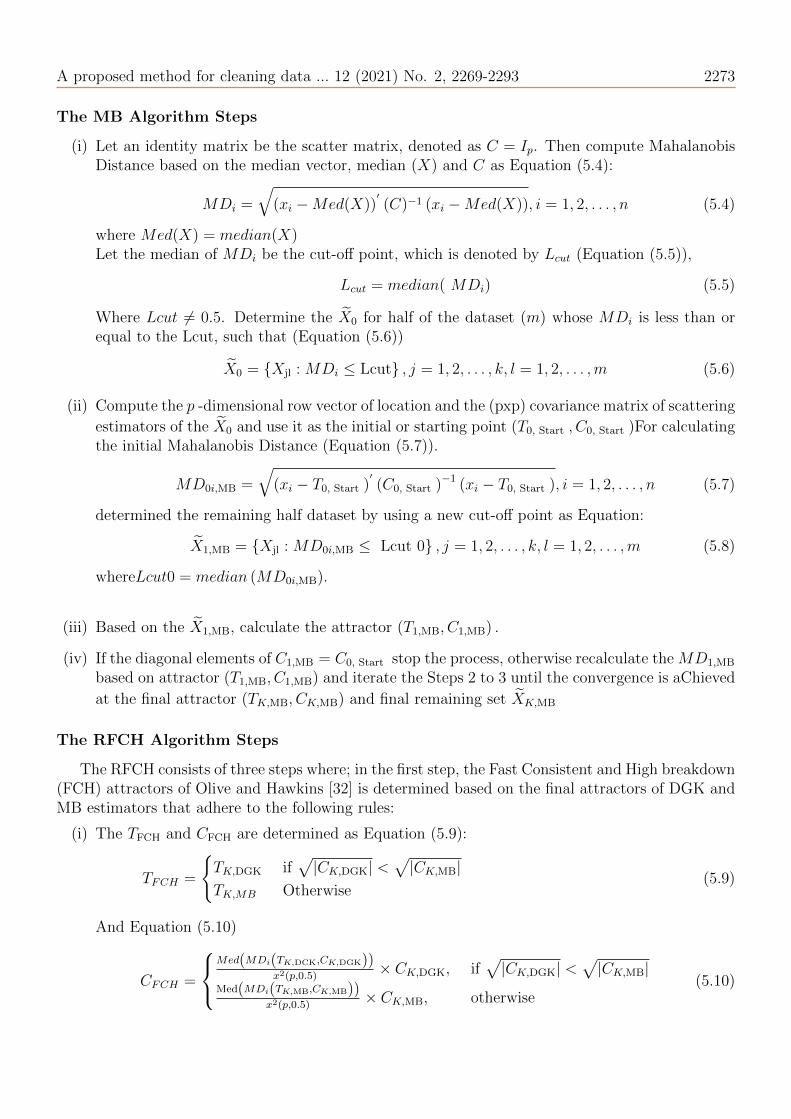
The MB Algorithm Steps

(i) Let an identity matrix be the scatter matrix, denoted as C = Ip. Then compute MahalanobisDistance based on the median vector, median (X) and C as Equation (5.4):

MDi =

√(xi −Med(X))

′(C)−1 (xi −Med(X)), i = 1, 2, . . . , n (5.4)

where Med(X) = median(X)Let the median of MDi be the cut-off point, which is denoted by Lcut (Equation (5.5)),

Lcut = median( MDi) (5.5)

Where Lcut = 0.5. Determine the X0 for half of the dataset (m) whose MDi is less than orequal to the Lcut, such that (Equation (5.6))

X0 = {Xjl : MDi ≤ Lcut} , j = 1, 2, . . . , k, l = 1, 2, . . . ,m (5.6)

(ii) Compute the p -dimensional row vector of location and the (pxp) covariance matrix of scattering

estimators of the X0 and use it as the initial or starting point (T0, Start , C0, Start )For calculatingthe initial Mahalanobis Distance (Equation (5.7)).

MD0i,MB =

√(xi − T0, Start )

′(C0, Start )

−1 (xi − T0, Start ), i = 1, 2, . . . , n (5.7)

determined the remaining half dataset by using a new cut-off point as Equation:

X1,MB = {Xjl : MD0i,MB ≤ Lcut 0} , j = 1, 2, . . . , k, l = 1, 2, . . . ,m (5.8)

whereLcut0 = median (MD0i,MB).

(iii) Based on the X1,MB, calculate the attractor (T1,MB, C1,MB) .

(iv) If the diagonal elements of C1,MB = C0, Start stop the process, otherwise recalculate theMD1,MB

based on attractor (T1,MB, C1,MB) and iterate the Steps 2 to 3 until the convergence is aChieved

at the final attractor (TK,MB, CK,MB) and final remaining set XK,MB

The RFCH Algorithm Steps

The RFCH consists of three steps where; in the first step, the Fast Consistent and High breakdown(FCH) attractors of Olive and Hawkins [32] is determined based on the final attractors of DGK andMB estimators that adhere to the following rules:

(i) The TFCH and CFCH are determined as Equation (5.9):

TFCH =

{TK,DGK if

√|CK,DGK| <

√|CK,MB|

TK,MB Otherwise(5.9)

And Equation (5.10)

CFCH =

Med(MDi(TK,DCK,CK,DGK))

x2(p,0.5)× CK,DGK, if

√|CK,DGK| <

√|CK,MB|

Med(MDi(TK,MB,CK,MB))x2(p,0.5)

× CK,MB, otherwise(5.10)


where x2(p,0.5) is Chi-square distribution with p degrees of freedom and significance level 0.5.

The (TFCH, C∗FCH) are the consistent estimators of the FCH attractors according to Theorem 1

of Olive and Hawkins [32],

where C∗FCH =

Med (MDi (TFCH, CFCH))

x2(p, 0.5)∗ CFCH.

(ii) Construct a new set of data, XFCH by using the following Equation (5.11),

XFCH ={Xjl : MDi (TFCH, C

∗FCH) ≤ x2

(p,1−α)

}, j = 1, 2, . . . , k, l = 1, 2, . . . ,m, (5.11)

where MDi (TFCH, C∗FCH) is the Mahalanobis Distance based on the location and scatter of FCH

estimators in (i) . Then compute the location and scatter estimators for the XFCH dataset toobtain the RFCH attractors, (T1,RFCH, C1,RFCH) · Again, following Theorem 1 of Olive andHawkins [32], C∗

1,RFCH is defined as Equation (5.12),

C∗1,RFCH =

Med (MDi (T1,RFCH, C1,RFCH))

x2(p, 0.5)∗ C1,RFCH (5.12)

Subsequently, the Mahalanobis Distance based on is computed, and a new set of data is con-structed using the following Equation;

X2,RFCH ={Xjl : MDi

(T1,RFCH, C

∗1,RFCH

)≤ x2(p, 1− α)

},

j = 1, 2, . . . , k, l = 1, 2, . . . ,m(5.13)

Following the same process, (T2,RFCH, C2,RFCH) estimators are calculated based on the X2,RFCH

dataset. Afterward, C∗2,RFCH is defined as in Equation (5.14) by applying Theorem 1 of Olive

and Hawkins [32]

C∗2,RFCH =

Med (MDi (T2,RFCH, C2,RFCH))

x2(p, 0.5)∗ C2,RFCH (5.14)

(iii) Repeat steps (i)-(ii) with the new cut-off point until convergence to get the final attractors

(TRFCH, CRFCH) and XRFCH , Subsequently, the Mahalanobis Distance based on is computed,and a new set of data is constructed using the following Equation (5.15)

clean data robust =X3,RFCH ={Xjl : MDi

(T2,RFCH, C

∗2,RFCH

)≤ x2(p, 1− α)

},

j = 1, 2, . . . , k, l = 1, 2, . . . ,m(5.15)

Upon convergence, the RFCH produced the final (TRFCH, CFCH) estimators which are√n Consistent

according to [32, 30, 48, 60, 59, 38, 19, 34, 33].

6. Structural Equation Models (SEM)

An important two-part of models employed in SEM includes measurement models and structuremodels. CFA is used to correct for indicator measurement error, shaping the latent variables (factors).A model in which the exogenous variable x and the endogenous variables y are being measured isdefined as

x = Λxξ + δ

y = Λyη + ε(6.1)


The full structural Equation model is defined as

η = Bη + Γξ + ζ

(I−B) η = Γξ + ζ

η = (I−B)−1(Γξ + ζ)

(6.2)

The covariance matrix is obtained as follows by

Σ(θ) =

[Λy(I−B)−1[ΓΦΓ

′+Ψ](I−B)−1Λ

′y +Θε Λy(I−B)−1ΓΦΛ

′x

ΛxΦΓ′(I−B)−1Λ

′y ΛxΦΛ

′x +Θδ

](6.3)

Therefore the matrix of covariance was proven [46, 13, 7].

7. Estimation of Model Parameters

7.1. The maximum likelihood function for SEM (ML)

Several frequently used estimation methods for structural equation modeling have already beenwell established and are commonly employed. Maximum likelihood estimators are the most oftenused normal theory estimators in SEM (ML). The vast majority of the most widely used softwarepackages rely on ML as their default estimator. The iterative process with a variational minimizationtechnique aims to generate a function that can expect the target value. The fit function may bedefined differently. The first approach uses a log-likelihood ratio fit that minimizes a multivariatenormality assumption to address the problem. The second technique is based on a form general ofthe for least-squares fit function.

An examination of a multivariate normal population through the use of a random sample wouldindicate that a random sampling procedure called Wishart distribution (Wishart 1928) allows calcu-lating the probability of selecting a sample with variance-covariance matrix S.

S =1

N − 1

N∑i=1

(xij − xj)(xij − xj)′=

1

n

N∑i=1

(xij − xj)(xij − xj)′

(7.1)

The maximization of the equation is equivalent to the minimization of the function in brackets:

FML(θ) = ln |Σ|+ tr(SΣ−1)− ln |S| − (p+ q) (7.2)

While q denotes the X variable and p denotes the Y variable.While θ is the parameter vector, Σ is the covariance matrix implied by the model,

FML denotes the fitting function’s value as determined at the final estimates.,|Σ| is the determinant of a matrix, while tr is the matrix’s trace [7].

Efficient and consistent estimates of unknown parameters are achieved by minimizing the Eq. (7.2).

θML = argminFML(S, Σ(θ) = ln |Σ(θ)|+ tr|Σ(θ)| − ln |S| − (k) (7.3)

As equation (7.3) shows, at the minimum of the fit function FML(θ), θML contains parameter estimatesΛ,Φ, and Ψ, where Λ is a matrix of estimated factor loadings, Φ is an estimated factor covariance, andΨ is the covariance matrix of error variables. Γ is the matrix structural regression of the endogenousand latent exogenous variables, B regression between endogenous factors latent. Standard errors


are defined as the square roots of the diagonal elements of the approximation asymptotic covarianceproduced from ML under multivariate normality assumption:

acov(Θ)ML =

(2

N − 1

){E

[∂2FML

∂θ∂θ′ |θ=θ0

]}−1

= n−1(∆

′Γ−1∆

)−1

(7.4)

where Γ = Γ(ij,kl) = σikσjl + σilσjk and ∆ = (∂σ(θ)/∂θ′)|θ=θ0

.And Is the model’s partial derivatives matrix as respects the parameters Estimates of parameters

provided by ML are desirable asymptotic, such as unbiased, consistency and efficiency in addition InSEM, A fundamental aspect of modeling is determining how well a model fits a situation Model fitis evaluated using the Chi-square goodness. which is a function of the fit and may be calculated asfollows:

TML = (N − 1)FML, df = s− t (7.5)

Represent s is the number of non-duplicated components in the observable covariance matrix s =12k(k + 1) and t is the count of unknown parameters and a χ2 distribution with s − t degrees of

freedom [18, 7, 40, 53, 3, 2].

7.2. Generalized least squares(GLS)

The generalized least squares (GLS) method, based on normal theory, first debuted in 1970 (e.g.,Anderson, 1973)[11], and has since been widely used. Suppose {x1, . . . , xn} are samples of x suchthat all xi are (iid) according to N [0,Σ] . The covariance matrix is

S = (n− 1)−1

n∑i=1

(xi − x) (xi − x)′

(7.6)

This is the most basic finding for constructing the theory of Covariance Structure Analysis underthe normally distributed assumption. A result is obtained by Equation (7.7)

n1/2vec (S − Σ) = n12k−′

vecs (S − Σ)L−→ N

[0, 2k−′

k′(Σ⊗ Σ) kk−

]= N [0, 2D (Σ⊗ Σ)D]

(7.7)

Another important matrix D (k2 × k2) is defined by D = kk− = k(k

′k)−1

k′.

The GLS function is expressed in terms of the residual quadratic form:

(vecs(S − Σ))′(2n−1k

′(Σ0 ⊗ Σ0) k

)−1

(vecs(S − Σ)) (7.8)

Because Σ If unknown, we will substitute by k ∗ k positive definite matrices V. A discrepancy wasidentified and explored via [10], known as the Generalized Least Squares (GLS). the GLS function is

FGLS(θ) =1

2

[vec(S − Σ(θ))

′(V ⊗ V )vec(S − Σ(θ))

]=

1

2tr[(S − Σ(θ))V ]2 (7.9)

. The constant positive definitive matrix V is a k × k or the stochastic matrix V that is more likelythan not to converge in probability to the constant positive definitive matrix V ∗. It is represented bythe symbol V*, where vec() is a vectorization operator that turns a matrix into a vector by stakingrows of the matrix, where ⊗ is the Kronecker product [28]. When V converges in probability toΣ−1. [10, 11], demonstrated that the GLS estimator θGLS that minimizes FGLS(θ) is asymptotically

identical to θML and TGLS = (n− 1)FGLS

(θ), and df = s− t degree of freedom with χ2 distribution

is used to describe nFGLS(θ)L−→ χ2

s−t [24, 26, 35].


7.3. Maximum likelihood robust function for SEM (MLR)

Because the assumption of normality is invalid, ML estimates for parameters are not asymp-totically effective. Due to faulty asymptotic covariance matrix assumption, the Cov(θ)ML from

equation acov(Θ)ML = ( 2N−1

){E[ ∂2FML

∂θ∂θ′ |θ=θ0]}

−1= n−1

(∆

′Γ−1∆

)−1is no longer consistent with the

corresponding true covariance matrix, resulting in incorrect standard error estimations. An affirma-tive, creative response is to be expected.” It has been shown by [56, 58], that Modeling parameterswith MLR have a comparable estimation method to ML. Still, additional adjustments are made toensure robustness against nonnormal data. The correction of SB scaling (Satorra and Bentler, 1994)and [54] can be applied if the model is unspecified or data is the outlier.

Browne’s (1982, 1984) original residual-based test statistics TB Has a theoretical benefit: if thesample size is large enough, the distribution of the test statistics is known exactly. The estimate θ:is given as follows:

TB

(θ)= ne

′σc

(θ) [

σ′

c

(θ)SY σc

(θ)]−1

σ′

c

(θ)e (7.10)

where σ(θ) = ∂σ(θ)/∂θ or σ(θ) = ∂vechΣ(θ)/∂θ represents the Jacobian matrix s× t. There is nowan s× (s− t) matrix σc(θ) with columns that are orthogonal with those of σ(θ). To guarantee thatthe model is accurately identified at θ, we assume that σ(θ) has complete rank in the vicinity ofθ, represented by σ = σ(θ). And e = s − σ(θ) represents the disparity between the data and anyconsistent estimator-estimated model.

[54] proposed the TYB test statistic, a modified residual-based test statistic. The concept origi-nates in the regression literature, where model residual cross-products estimate asymptotic covariancematrix and standard errors [22]. With the ofΓ replace SY , the following decomposition can be usedto obtain a consistent estimate θ

Γ =1

n

N∑i=1

[Yi − σ(θ)

] [Yi − σ(θ)

]′= SY +

N

n[Y − σ(θ)][Y − σ(θ)]

′(7.11)

Replacing SY in (7.10) by Γ, the Yuan-Bentler residual-based statistic is given by:

TYB(θ) = TB(θ)/[1 +NTB(θ)/n

2)]

(7.12)

Additionally, the approximate theoretical result of the χ2 distribution with (s− t)) degrees of freedomare also realized asymptotically.However TYB(θ) < TB(θ), given any consistent estimate θ, it is believed that the problem of overrejection will be reduced by using TYB. Because the denominator in (7.12) is nearly always biggerthan one, which tends to minimize inflation, it will be small and help reduce it though. [22] observedthat nominal TYB has a high rate of model acceptance even in the face of limited sample size [47, 43].

Another way to express the correction for standard errors. There is always a need to rescuethe standard errors. Note Asparouhov and Muthen (2005) methods that the parameter covariancematrix under the multivariate normality assumption is defined by Equation acov(Θ)ML , whereasthe robust parameter covariance matrix has a sandwich-like form under non-normality, as shown inEquation (7.13)

cov(√Nθ) =

(∆

′Γ−1∆

)−1

∆′Γ−1Γ∗Γ−1∆

(∆

′Γ−1∆

)−1

(7.13)

is the matrix above of model derivatives evaluated at the parameters estimates And Γ∗ is thekurtosis matrix of the data, or a distribution-free estimate of the asymptotic covariance matrix of


sample covariances [10]. The typical element Γ∗ , is Γ∗ij,kl = sijkl − sijskl Where sijkl is the fourth

central moment of the data observed, and sij, skl are covariances of samples. [36] The inverse matrix

of Fisher information (∆′Γ−1∆)

−1Which is similar to Equation (7.13), forms the outer ”bread” of the

sandwich, and the inner part (i.e., the ”meat”) is ∆′Γ−1Γ∗Γ−1∆, where Γ∗ It is the same as the ADF

asymptotic covariance matrix, which can be defined based on Equation Γ∗ = Γ∗ij,kl = σijkl−σijσkl. And

this matrix of covariance is sometimes called the ”covariance matrix for a sandwich” [53, 39, 10, 54],rewrite the

acov(θ) = N−1AMLRBMLRAMLR, (7.14)

8. Model Evaluation

Researchers use total fit indices from studies in applied SEM to make decisions on model-data fit.is applied to the primary hypothesis Σ(θ) = Σ. If the model-estimated variance/covariance matrix,Σ Is not significantly different from the actual data covariance matrix, S, then we say the modelfits the data well. All research has found the following: The overall model fit is evaluated beforeparameter estimations are interpreted. The results of the sample estimates are unreliable until themodel has been validated [7, 1, 23].

8.1. Root Mean Square Error of Approximation (RMSEA) Index

Some practical research considers the (RMSEA) to be one of the most useful and reliable mea-sures of model fit. The RMSEA was first created by ( Steiger & Lind, 1980) ). If the populationcovariance matrix were available, the RMSEA would tell you how well the hypothesized model wouldfit the population covariance matrix with randomly selected parameter valuesThe RMSEA fit indexis determined as follows

RMSEAML,n =

√√√√max

(0,

F (S,Σ(θ))

df− 1

n− 1

)=

√max

(0,

T,n − df

(n− 1)df

)(8.1)

F (S,Σ(θ)) denotes that the fit function is minimized, while max denotes the maximum value of thebracketed values, and The number of known parameters is s. In contrast, the number of independentparameters ist. The degree of freedom is denoted by df = s− t , and the sample size is denoted byn [41]. A good fit index is when the value is less than 0.05. In equation (8.5), when the sample sizeis large compared to the model size, RMSEA produces superior estimate performance. When thesample size is large, the term [1/(n – 1)] approaches 0 asymptotically [37, 12, 51, 36].

8.2. Comparative Fit Index (CFI)

Bentler (1990) suggested the CFI as another incremental fit index. For the ML-based CFI, thefollowing are the population and sample definitions:

CFIn = 1− F0,M

F0,B

= 1− TM − dfMTB − dfB

, or 1− max [(TM − dfM) , 0]

max [(TM − dfM) , (TB − dfB) , 0](8.2)

If the population and the sample values of the ML discrepancy of the model are F0,B and FB;

if the baseline model. χ2B represent Chi-square of the baseline model, F represents the minimum fit

function and χ2M represent Chi-square of the target model.

This test compares your model’s predicted covariance matrix against the null model’s observedcovariance matrix. The CFI value ranges from 0 to 1. A CFI score close to 1 suggests that the modelis well fitted. The cut-off for a satisfactory fit for a CFI value is > 90 [1], suggesting that your modelcan recreate 90% of the covariance in the data. CFI is unaffected by sample size [17, 41, 42, 15].


8.3. Tucker Lewis Index (TLI)

TLI, the incremental fit index developed by Tucker and Lewis (1973) originally, was a reliabilitycoefficient named after [1]. To compare nested or non-nested models inside any sample or compare aparticular model across samples with differing sizes, the researchers employed TLI (sometimes calledNNFI, or Nonnormed Fit Index)[1]. TLI is defined as

TLIM,n = 1− TM − dfMTB − dfB

× dfBdfM

= 1− [(λM/dfM)/(λB/dfB)] (8.3)

TML,B represent Chi-square of the baseline model, FML,M represent the minimum fit function andTML,M Represent Chi-square of the target model. The TLI approaches 1 for a correctly describedmodel; however, the TLI can surpass the range of 0 to 1. The poorer the fit of the model, the smallerthe value being modeled. When the TLI number was larger, the model was more suited. Most studieschoose 0.97 as the cut-off threshold, but values of 0.95 or above are usually acceptable. [14, 22, 51].

8.4. Robust Model-fit Indexes with methods robust estimation

The robust Chi-square statistic, resilient to no normal data, corrects the other Chi-square-basedgoodness-of-fit indices such as RMSEA, CFI, and TLI. According to [36]. Another method is usingnonnormal data from the robust RMSEA. When requested to use Yuan and Bentler’s robust MLtechnique (1999), these programs print a robust RMSEA, different from Equation (8.1). This robustRMSEA is calculated according to the equation below:

RMSEAPR,n =

√max(0,

TY B,n − df

(n− 1)df) (8.4)

This equation is obtained by simply replacing TML,n;n in Equation (8.2) and (8.3) with TY B,n.one can replace T with TML, TMLR, For the CFI and the TLI,

CFIY B,n = 1− TY B,M − dfMTY B, B − dfB

(8.5)

TLIY B,n = 1−TY B,M − dfMTY B, B − dfsB

× dfBdfM

[8, 9] (8.6)

while FM and dM are the fit function and degrees of freedom, respectively. Model Baseline denotesB. [8, 52, 22].

9. Residual-Based Fit Indices

9.1. Residual Matrix

. Residual matrix To examine the hypothesis that Σ = Σ(θ) you must calculate Σ − Σ(θ). Anonzero member in a null matrix indicates model definition error. To find S, you would use Σ(θ) asa substitution for Σ, and then you would use S − Σ(θ) to form Σ − Σ(θ) has elements, where eachelement is calculated as Σ − Σ(θ). The sample correlation is rij − ρij, while the model predictedcorrelation is rij − ρij. While this fix adequately tackles scaling discrepancies, it neglects samplinginaccuracy. the correlation residuals the following [21, 7].

rij − ρij =sij

(siisjj)1/2

− σij

(σiiσjj)1/2

, (i, j = 1, . . . , p) (9.1)


9.1.1. Standardized Root Mean square Residual (SRMR)

This formula is known as the ”Root Mean Square Residual” (SRMR). Dr. Bentler created SRMRin 1995, [3]. It is a covariance residual-based indicator of fit, calculated as the covariance residualsdifference between observed and model projected covariances. Residuals should ideally be approaCh-ing zero as long as the researcher’s model fits the data adequately. SRMR resulted in a correlationmatrix for the sample and predicted covariance matrix and then applies the procedure for calcu-lating mean total correlation residuals. Thus, SRMR accounts for both the actual and anticipatedcorrelations [25]. SRMR is calculated the sample estimate and population its are as follows:

SRMR =

√√√√1

s

p∑i=1

i∑j=1

(σ∗ij − σ0,ij

)2σ∗iiσ

∗y

(9.2)

Where s = k(k + 1)/2). And σ∗ij, σ0,ij, are elements of Σ∗and Σ0 Respectively. SRMR value has 0 or

1, with 0 being the optimum fit and 1 representing the worst fit. [15, 25, 41].

9.1.2. Correlation Root Mean Square Residual (CRMR)

Another standardized effect size of overall misfit suitable for covariance structure models is thecorrelation root mean square residual (CRMR):

CRMR =

√1

s− p

∑i<j

(ρij − ρ0ij

)2(9.3)

Where s = k(k + 1)/2) and p represent vector sample variances. If you have an unknowncorrelation between variables, ρij describes the correlation between variables i and j and ρ0ij indicatesthe correlation for the model fit. For the sake of ease of interpretation, standardized effect sizes arepreferred to unstandardized effect sizes. [29, 31, 44].

10. Characteristics of the Research Summary

The features of the research summary dictate how the quality of the simulation findings is evalu-ated. The preceding robustness analysis used the following study summary data. The term ”relativebias” refers to the bias of parameter estimators calculated by the equation following

Bias(θi

)=

θi − θiθi

, (10.1)

where θi denotes the population value for ith parameter and θi Denotes the mean of the ith parameterestimations across all replications. For parameter estimation, the mean absolute relative bias is

1

t

t∑i=1

∣∣∣Bias(θi

)∣∣∣ , (10.2)

The number of parameters in the model is denoted by t. The relative bias of estimators for parameterstandard errors θi It is defined as Represent t is the number of parameters in the model. The relativebias of estimators for the standard error of parameter estimates θi is calculated by equation

Bias(se(θi

))=

se(θi

)− sd

(θi

)sd(θi

) , (10.3)


where sd(θi

)Denotes the standard deviation of the estimates for the parameter I, and (se( i ) )

denotes the mean of the standard error estimates for the parameter I across all replications. Forstandard error estimation, the mean absolute relative bias is

1

t

t∑i=1

∣∣∣Bias(se(θi

))∣∣∣ , (Harwell, 2018) (10.4)

11. Simulation at the Population Level

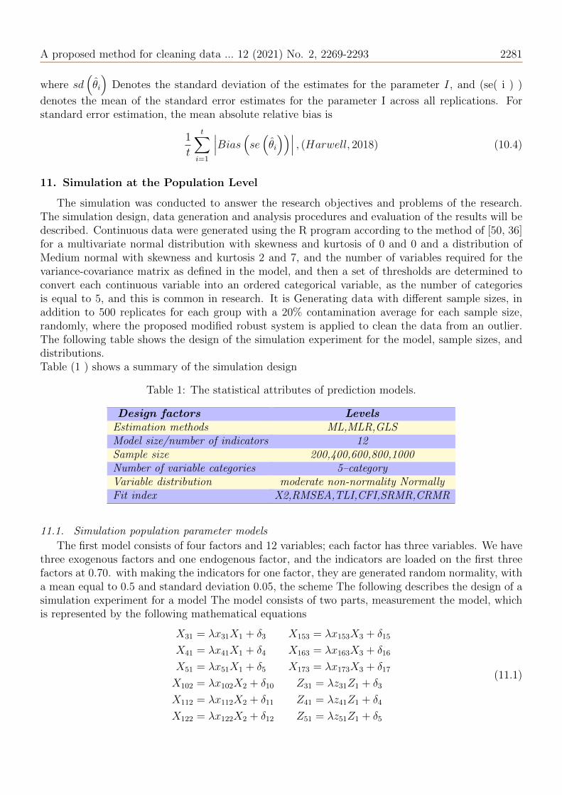
The simulation was conducted to answer the research objectives and problems of the research.The simulation design, data generation and analysis procedures and evaluation of the results will bedescribed. Continuous data were generated using the R program according to the method of [50, 36]for a multivariate normal distribution with skewness and kurtosis of 0 and 0 and a distribution ofMedium normal with skewness and kurtosis 2 and 7, and the number of variables required for thevariance-covariance matrix as defined in the model, and then a set of thresholds are determined toconvert each continuous variable into an ordered categorical variable, as the number of categoriesis equal to 5, and this is common in research. It is Generating data with different sample sizes, inaddition to 500 replicates for each group with a 20% contamination average for each sample size,randomly, where the proposed modified robust system is applied to clean the data from an outlier.The following table shows the design of the simulation experiment for the model, sample sizes, anddistributions.Table (1 ) shows a summary of the simulation design

Table 1: The statistical attributes of prediction models.

Design factors LevelsEstimation methods ML,MLR,GLSModel size/number of indicators 12Sample size 200,400,600,800,1000Number of variable categories 5–categoryVariable distribution moderate non-normality NormallyFit index X2,RMSEA,TLI,CFI,SRMR,CRMR

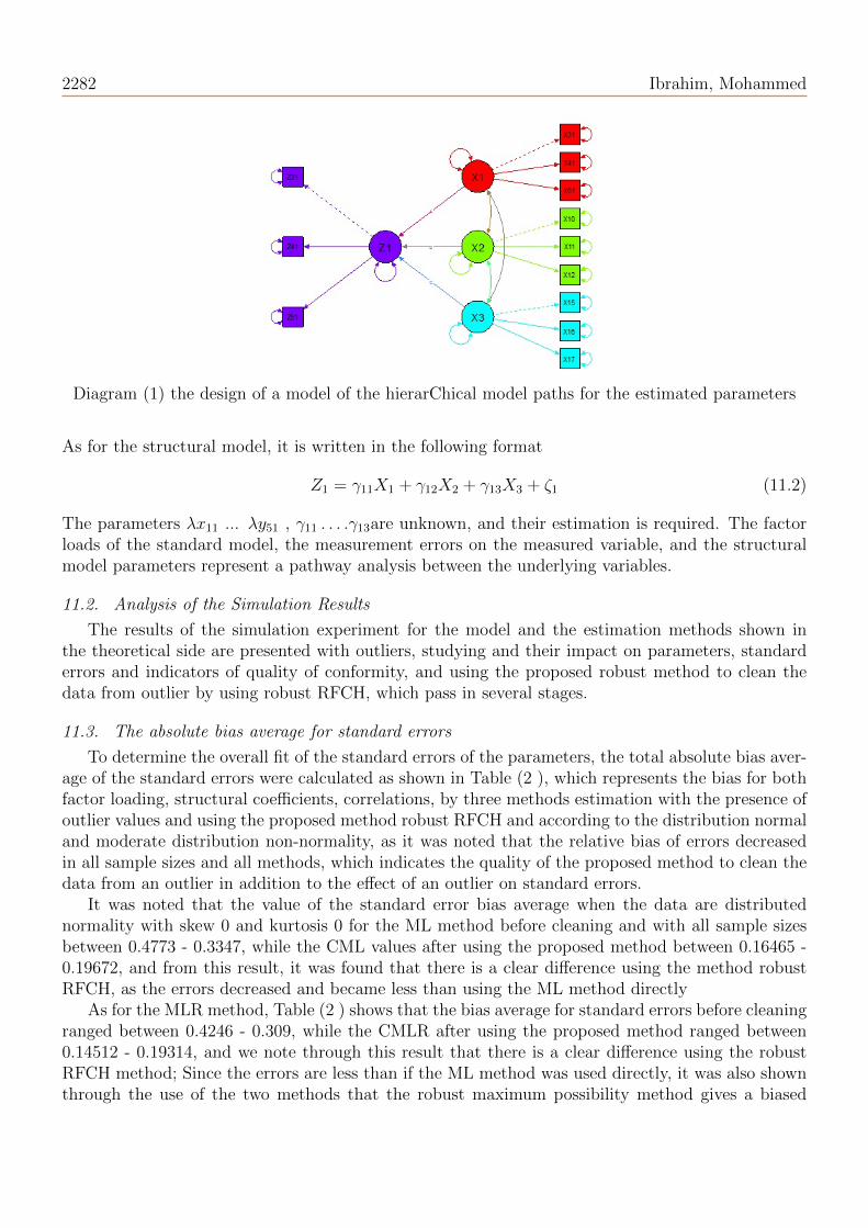
11.1. Simulation population parameter models

The first model consists of four factors and 12 variables; each factor has three variables. We havethree exogenous factors and one endogenous factor, and the indicators are loaded on the first threefactors at 0.70. with making the indicators for one factor, they are generated random normality, witha mean equal to 0.5 and standard deviation 0.05, the scheme The following describes the design of asimulation experiment for a model The model consists of two parts, measurement the model, whichis represented by the following mathematical equations

X31 = λx31X1 + δ3 X153 = λx153X3 + δ15

X41 = λx41X1 + δ4 X163 = λx163X3 + δ16

X51 = λx51X1 + δ5 X173 = λx173X3 + δ17

X102 = λx102X2 + δ10 Z31 = λz31Z1 + δ3

X112 = λx112X2 + δ11 Z41 = λz41Z1 + δ4

X122 = λx122X2 + δ12 Z51 = λz51Z1 + δ5

(11.1)


Diagram (1) the design of a model of the hierarChical model paths for the estimated parameters

As for the structural model, it is written in the following format

Z1 = γ11X1 + γ12X2 + γ13X3 + ζ1 (11.2)

The parameters λx11 ... λy51 , γ11 . . . .γ13are unknown, and their estimation is required. The factorloads of the standard model, the measurement errors on the measured variable, and the structuralmodel parameters represent a pathway analysis between the underlying variables.

11.2. Analysis of the Simulation Results

The results of the simulation experiment for the model and the estimation methods shown inthe theoretical side are presented with outliers, studying and their impact on parameters, standarderrors and indicators of quality of conformity, and using the proposed robust method to clean thedata from outlier by using robust RFCH, which pass in several stages.

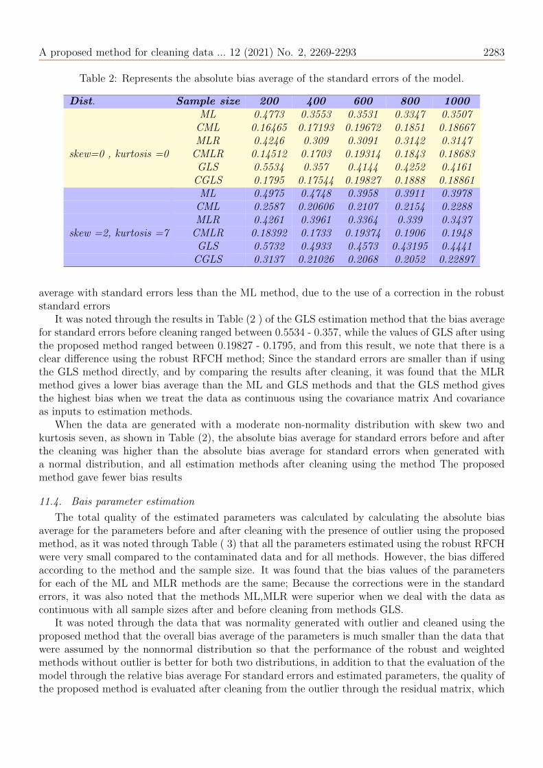
11.3. The absolute bias average for standard errors

To determine the overall fit of the standard errors of the parameters, the total absolute bias aver-age of the standard errors were calculated as shown in Table (2 ), which represents the bias for bothfactor loading, structural coefficients, correlations, by three methods estimation with the presence ofoutlier values and using the proposed method robust RFCH and according to the distribution normaland moderate distribution non-normality, as it was noted that the relative bias of errors decreasedin all sample sizes and all methods, which indicates the quality of the proposed method to clean thedata from an outlier in addition to the effect of an outlier on standard errors.

It was noted that the value of the standard error bias average when the data are distributednormality with skew 0 and kurtosis 0 for the ML method before cleaning and with all sample sizesbetween 0.4773 - 0.3347, while the CML values after using the proposed method between 0.16465 -0.19672, and from this result, it was found that there is a clear difference using the method robustRFCH, as the errors decreased and became less than using the ML method directly

As for the MLR method, Table (2 ) shows that the bias average for standard errors before cleaningranged between 0.4246 - 0.309, while the CMLR after using the proposed method ranged between0.14512 - 0.19314, and we note through this result that there is a clear difference using the robustRFCH method; Since the errors are less than if the ML method was used directly, it was also shownthrough the use of the two methods that the robust maximum possibility method gives a biased


Table 2: Represents the absolute bias average of the standard errors of the model.

Dist. ,Sample size 200 400 600 800 1000, ML 0.4773 0.3553 0.3531 0.3347 0.3507, CML 0.16465 0.17193 0.19672 0.1851 0.18667, MLR 0.4246 0.309 0.3091 0.3142 0.3147

skew=0 , kurtosis =0 , CMLR 0.14512 0.1703 0.19314 0.1843 0.18683, GLS 0.5534 0.357 0.4144 0.4252 0.4161, CGLS 0.1795 0.17544 0.19827 0.1888 0.18861, ML 0.4975 0.4748 0.3958 0.3911 0.3978, CML 0.2587 0.20606 0.2107 0.2154 0.2288, MLR 0.4261 0.3961 0.3364 0.339 0.3437

skew =2, kurtosis =7 , CMLR 0.18392 0.1733 0.19374 0.1906 0.1948, GLS 0.5732 0.4933 0.4573 0.43195 0.4441, CGLS 0.3137 0.21026 0.2068 0.2052 0.22897

average with standard errors less than the ML method, due to the use of a correction in the robuststandard errors

It was noted through the results in Table (2 ) of the GLS estimation method that the bias averagefor standard errors before cleaning ranged between 0.5534 - 0.357, while the values of GLS after usingthe proposed method ranged between 0.19827 - 0.1795, and from this result, we note that there is aclear difference using the robust RFCH method; Since the standard errors are smaller than if usingthe GLS method directly, and by comparing the results after cleaning, it was found that the MLRmethod gives a lower bias average than the ML and GLS methods and that the GLS method givesthe highest bias when we treat the data as continuous using the covariance matrix And covarianceas inputs to estimation methods.

When the data are generated with a moderate non-normality distribution with skew two andkurtosis seven, as shown in Table (2), the absolute bias average for standard errors before and afterthe cleaning was higher than the absolute bias average for standard errors when generated witha normal distribution, and all estimation methods after cleaning using the method The proposedmethod gave fewer bias results

11.4. Bais parameter estimation

The total quality of the estimated parameters was calculated by calculating the absolute biasaverage for the parameters before and after cleaning with the presence of outlier using the proposedmethod, as it was noted through Table ( 3) that all the parameters estimated using the robust RFCHwere very small compared to the contaminated data and for all methods. However, the bias differedaccording to the method and the sample size. It was found that the bias values of the parametersfor each of the ML and MLR methods are the same; Because the corrections were in the standarderrors, it was also noted that the methods ML,MLR were superior when we deal with the data ascontinuous with all sample sizes after and before cleaning from methods GLS.

It was noted through the data that was normality generated with outlier and cleaned using theproposed method that the overall bias average of the parameters is much smaller than the data thatwere assumed by the nonnormal distribution so that the performance of the robust and weightedmethods without outlier is better for both two distributions, in addition to that the evaluation of themodel through the relative bias average For standard errors and estimated parameters, the quality ofthe proposed method is evaluated after cleaning from the outlier through the residual matrix, which


Table 3: The absolute bias average for the parameters of the model.

Dist. ,Sample size 200 400 600 800 1000, ML 30.0729 7.04054 6.0129 3.4046 1.44173, CML 2.062 0.22853 0.1869 0.19393 0.18904, MLR 30.0729 7.04054 6.0129 3.4046 1.44173


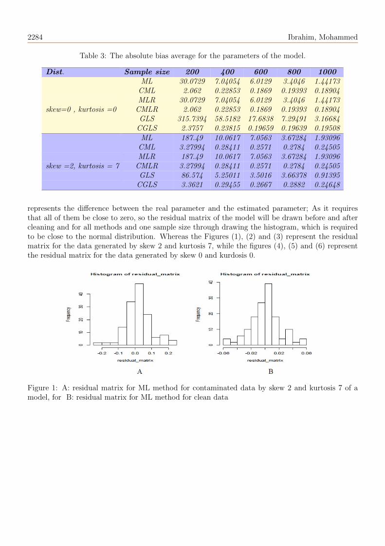
skew =2, kurtosis = 7 , CMLR 3.27994 0.28411 0.2571 0.2784 0.24505, GLS 86.574 5.25011 3.5016 3.66378 0.91395, CGLS 3.3621 0.29455 0.2667 0.2882 0.24648

represents the difference between the real parameter and the estimated parameter; As it requiresthat all of them be close to zero, so the residual matrix of the model will be drawn before and aftercleaning and for all methods and one sample size through drawing the histogram, which is requiredto be close to the normal distribution. Whereas the Figures (1), (2) and (3) represent the residualmatrix for the data generated by skew 2 and kurtosis 7, while the figures (4), (5) and (6) representthe residual matrix for the data generated by skew 0 and kurdosis 0.

Figure 1: A: residual matrix for ML method for contaminated data by skew 2 and kurtosis 7 of amodel, for B: residual matrix for ML method for clean data


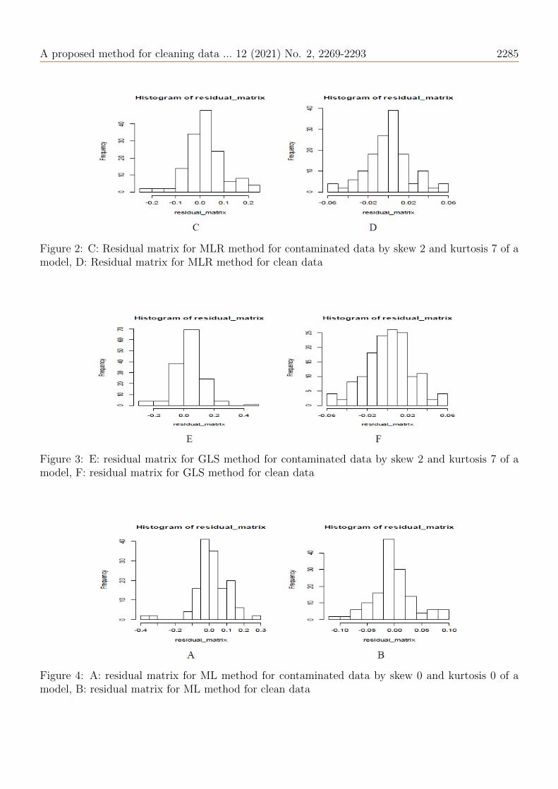
Figure 2: C: Residual matrix for MLR method for contaminated data by skew 2 and kurtosis 7 of amodel, D: Residual matrix for MLR method for clean data

Figure 3: E: residual matrix for GLS method for contaminated data by skew 2 and kurtosis 7 of amodel, F: residual matrix for GLS method for clean data

Figure 4: A: residual matrix for ML method for contaminated data by skew 0 and kurtosis 0 of amodel, B: residual matrix for ML method for clean data


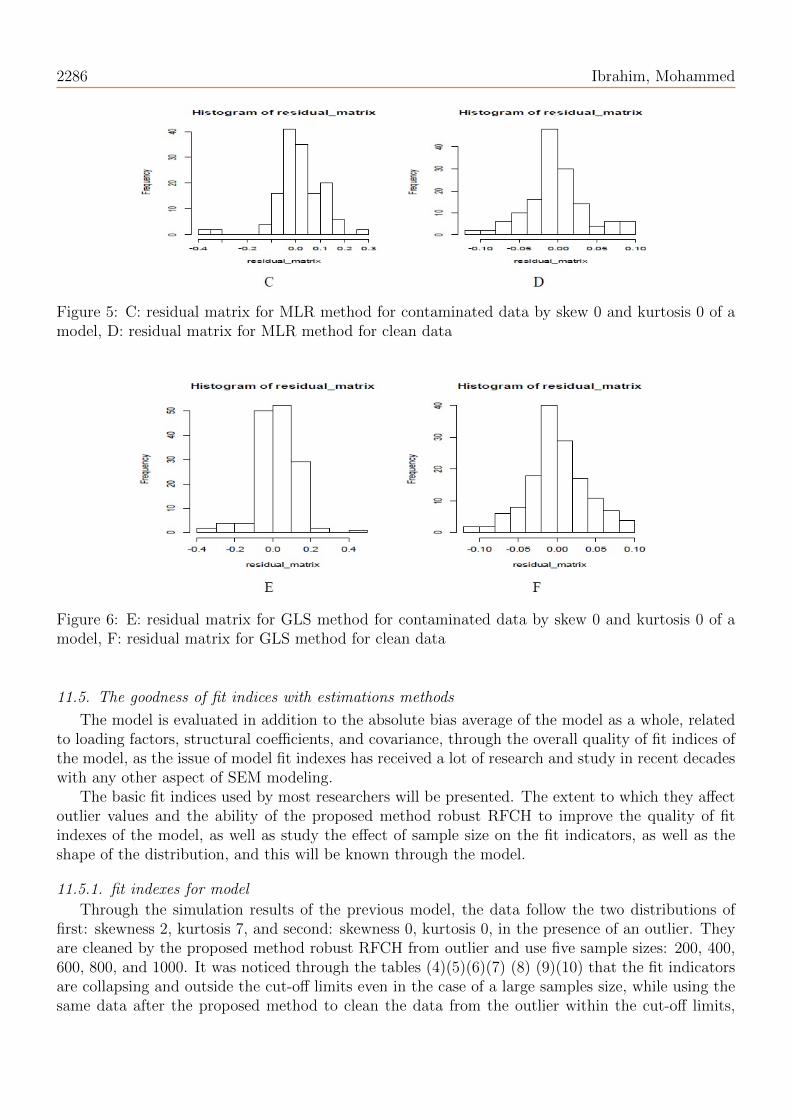
Figure 5: C: residual matrix for MLR method for contaminated data by skew 0 and kurtosis 0 of amodel, D: residual matrix for MLR method for clean data

Figure 6: E: residual matrix for GLS method for contaminated data by skew 0 and kurtosis 0 of amodel, F: residual matrix for GLS method for clean data

11.5. The goodness of fit indices with estimations methods

The model is evaluated in addition to the absolute bias average of the model as a whole, relatedto loading factors, structural coefficients, and covariance, through the overall quality of fit indices ofthe model, as the issue of model fit indexes has received a lot of research and study in recent decadeswith any other aspect of SEM modeling.

The basic fit indices used by most researchers will be presented. The extent to which they affectoutlier values and the ability of the proposed method robust RFCH to improve the quality of fitindexes of the model, as well as study the effect of sample size on the fit indicators, as well as theshape of the distribution, and this will be known through the model.

11.5.1. fit indexes for model

Through the simulation results of the previous model, the data follow the two distributions offirst: skewness 2, kurtosis 7, and second: skewness 0, kurtosis 0, in the presence of an outlier. Theyare cleaned by the proposed method robust RFCH from outlier and use five sample sizes: 200, 400,600, 800, and 1000. It was noticed through the tables (4)(5)(6)(7) (8) (9)(10) that the fit indicatorsare collapsing and outside the cut-off limits even in the case of a large samples size, while using thesame data after the proposed method to clean the data from the outlier within the cut-off limits,


which indicates that An improvement in the model by reducing errors as happened with parametersand standard errors, as well as it was noted that the fit indexes of differing according to the estimatedmethod Because some methods use the correction robust Chi-square, in addition, some fit indicatorsare based on the Chi-square correction robust.

11.5.2. Chi-square Fit Index

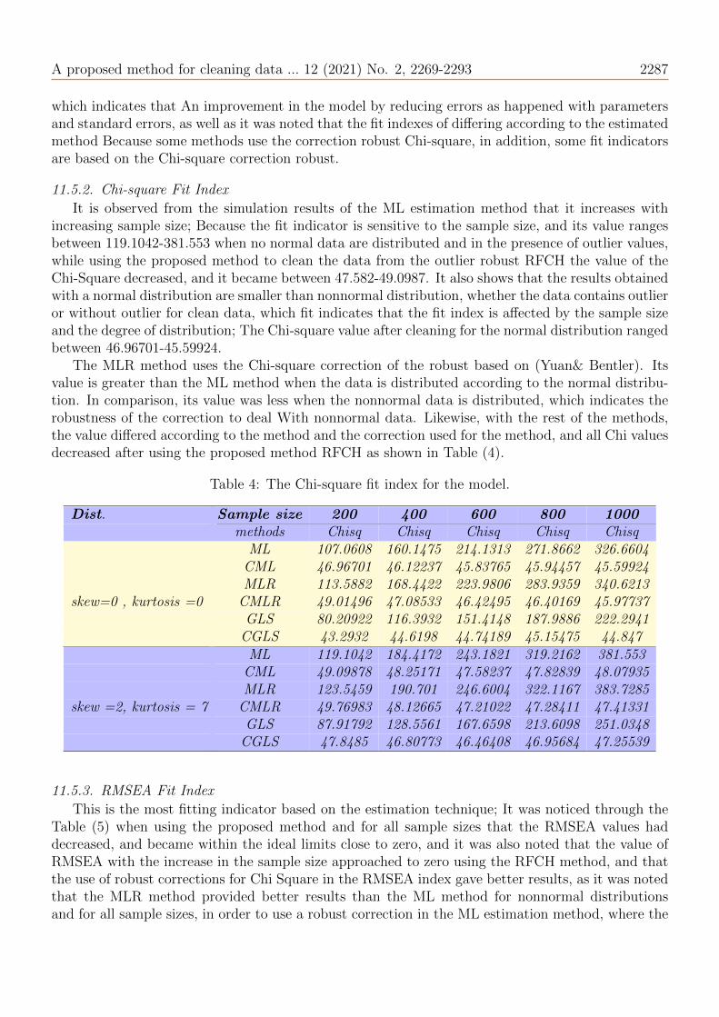
It is observed from the simulation results of the ML estimation method that it increases withincreasing sample size; Because the fit indicator is sensitive to the sample size, and its value rangesbetween 119.1042-381.553 when no normal data are distributed and in the presence of outlier values,while using the proposed method to clean the data from the outlier robust RFCH the value of theChi-Square decreased, and it became between 47.582-49.0987. It also shows that the results obtainedwith a normal distribution are smaller than nonnormal distribution, whether the data contains outlieror without outlier for clean data, which fit indicates that the fit index is affected by the sample sizeand the degree of distribution; The Chi-square value after cleaning for the normal distribution rangedbetween 46.96701-45.59924.

The MLR method uses the Chi-square correction of the robust based on (Yuan& Bentler). Itsvalue is greater than the ML method when the data is distributed according to the normal distribu-tion. In comparison, its value was less when the nonnormal data is distributed, which indicates therobustness of the correction to deal With nonnormal data. Likewise, with the rest of the methods,the value differed according to the method and the correction used for the method, and all Chi valuesdecreased after using the proposed method RFCH as shown in Table (4).

Table 4: The Chi-square fit index for the model.

Dist. ,Sample size 200 400 600 800 1000, methods Chisq Chisq Chisq Chisq Chisq, ML 107.0608 160.1475 214.1313 271.8662 326.6604, CML 46.96701 46.12237 45.83765 45.94457 45.59924, MLR 113.5882 168.4422 223.9806 283.9359 340.6213



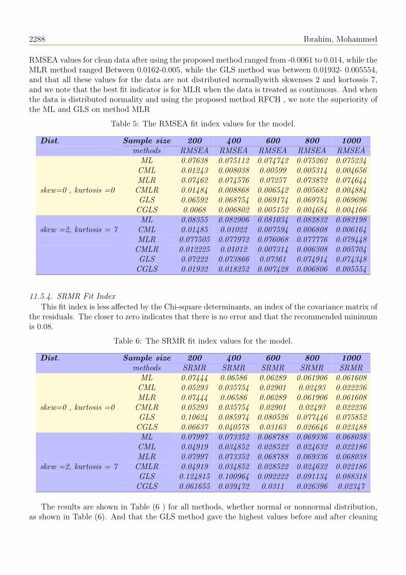
11.5.3. RMSEA Fit Index

This is the most fitting indicator based on the estimation technique; It was noticed through theTable (5) when using the proposed method and for all sample sizes that the RMSEA values haddecreased, and became within the ideal limits close to zero, and it was also noted that the value ofRMSEA with the increase in the sample size approached to zero using the RFCH method, and thatthe use of robust corrections for Chi Square in the RMSEA index gave better results, as it was notedthat the MLR method provided better results than the ML method for nonnormal distributionsand for all sample sizes, in order to use a robust correction in the ML estimation method, where the


RMSEA values for clean data after using the proposed method ranged from -0.0061 to 0.014, while theMLR method ranged Between 0.0162-0.005, while the GLS method was between 0.01932- 0.005554,and that all these values for the data are not distributed normallywith skwenses 2 and kortossis 7,and we note that the best fit indicator is for MLR when the data is treated as continuous. And whenthe data is distributed normality and using the proposed method RFCH , we note the superiority ofthe ML and GLS on method MLR

Table 5: The RMSEA fit index values for the model.

Dist. ,Sample size 200 400 600 800 1000, methods RMSEA RMSEA RMSEA RMSEA RMSEA, ML 0.07638 0.075112 0.074742 0.075262 0.075234, CML 0.01243 0.008038 0.00599 0.005314 0.004656, MLR 0.07462 0.074576 0.07257 0.073872 0.074644

skew=0 , kurtosis =0 , CMLR 0.01484 0.008868 0.006542 0.005682 0.004884, GLS 0.06592 0.068754 0.069174 0.069754 0.069696, CGLS 0.0068 0.006802 0.005152 0.004684 0.004166, ML 0.08355 0.082906 0.081034 0.082832 0.082198

skew =2, kurtosis = 7 , CML 0.01485 0.01022 0.007594 0.006808 0.006164, MLR 0.077505 0.077972 0.076068 0.077776 0.079448, CMLR 0.012225 0.01012 0.007314 0.006308 0.005704, GLS 0.07222 0.073866 0.07361 0.074914 0.074348, CGLS 0.01932 0.018252 0.007428 0.006806 0.005554

11.5.4. SRMR Fit Index

This fit index is less affected by the Chi-square determinants, an index of the covariance matrix ofthe residuals. The closer to zero indicates that there is no error and that the recommended minimumis 0.08.

Table 6: The SRMR fit index values for the model.

Dist. ,Sample size 200 400 600 800 1000, methods SRMR SRMR SRMR SRMR SRMR, ML 0.07444 0.06586 0.06289 0.061906 0.061608, CML 0.05293 0.035754 0.02901 0.02493 0.022236, MLR 0.07444 0.06586 0.06289 0.061906 0.061608



The results are shown in Table (6 ) for all methods, whether normal or nonnormal distribution,as shown in Table (6). And that the GLS method gave the highest values before and after cleaning


and for all sample sizes. In contrast, the ML and MLR method gives the same results, as it wasnoted that with the increase in the sample size and for all methods after cleaning, it approaches morethan zero and the least error for the residuals.

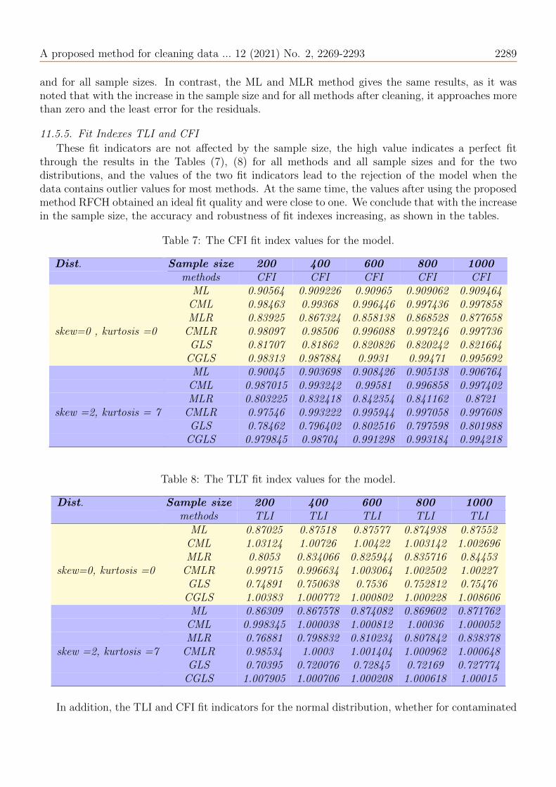
11.5.5. Fit Indexes TLI and CFI

These fit indicators are not affected by the sample size, the high value indicates a perfect fitthrough the results in the Tables (7), (8) for all methods and all sample sizes and for the twodistributions, and the values of the two fit indicators lead to the rejection of the model when thedata contains outlier values for most methods. At the same time, the values after using the proposedmethod RFCH obtained an ideal fit quality and were close to one. We conclude that with the increasein the sample size, the accuracy and robustness of fit indexes increasing, as shown in the tables.

Table 7: The CFI fit index values for the model.

Dist. ,Sample size 200 400 600 800 1000, methods CFI CFI CFI CFI CFI, ML 0.90564 0.909226 0.90965 0.909062 0.909464, CML 0.98463 0.99368 0.996446 0.997436 0.997858, MLR 0.83925 0.867324 0.858138 0.868528 0.877658



Table 8: The TLT fit index values for the model.

Dist. ,Sample size 200 400 600 800 1000, methods TLI TLI TLI TLI TLI, ML 0.87025 0.87518 0.87577 0.874938 0.87552, CML 1.03124 1.00726 1.00422 1.003142 1.002696, MLR 0.8053 0.834066 0.825944 0.835716 0.84453

skew=0, kurtosis =0 , CMLR 0.99715 0.996634 1.003064 1.002502 1.00227, GLS 0.74891 0.750638 0.7536 0.752812 0.75476, CGLS 1.00383 1.000772 1.000802 1.000228 1.008606, ML 0.86309 0.867578 0.874082 0.869602 0.871762, CML 0.998345 1.000038 1.000812 1.00036 1.000052, MLR 0.76881 0.798832 0.810234 0.807842 0.838378

skew =2, kurtosis =7 , CMLR 0.98534 1.0003 1.001404 1.000962 1.000648, GLS 0.70395 0.720076 0.72845 0.72169 0.727774, CGLS 1.007905 1.000706 1.000208 1.000618 1.00015

In addition, the TLI and CFI fit indicators for the normal distribution, whether for contaminated


data and clean data, after using the proposed method give greater results than if the data distributionis no normal.

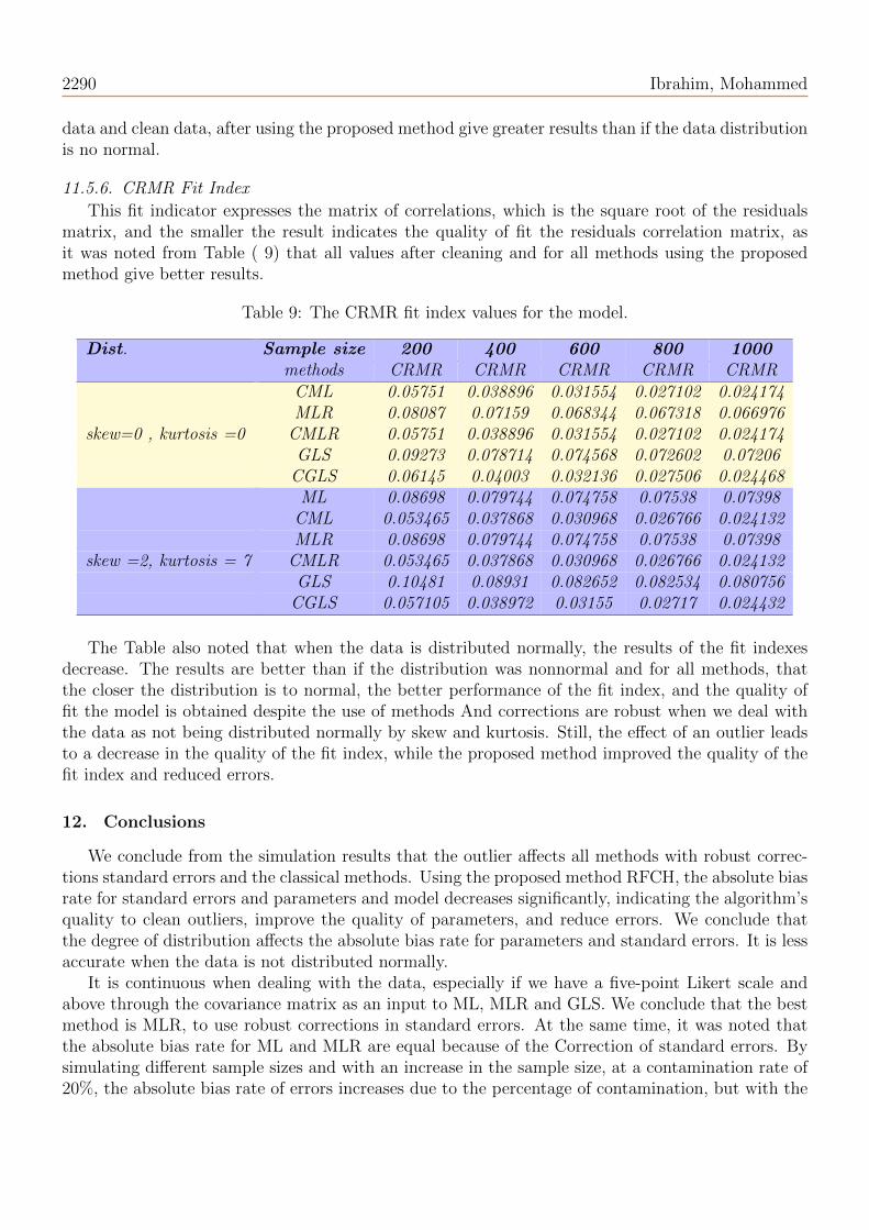
11.5.6. CRMR Fit Index

This fit indicator expresses the matrix of correlations, which is the square root of the residualsmatrix, and the smaller the result indicates the quality of fit the residuals correlation matrix, asit was noted from Table ( 9) that all values after cleaning and for all methods using the proposedmethod give better results.

Table 9: The CRMR fit index values for the model.

Dist. ,Sample size 200 400 600 800 1000, methods CRMR CRMR CRMR CRMR CRMR, CML 0.05751 0.038896 0.031554 0.027102 0.024174, MLR 0.08087 0.07159 0.068344 0.067318 0.066976



The Table also noted that when the data is distributed normally, the results of the fit indexesdecrease. The results are better than if the distribution was nonnormal and for all methods, thatthe closer the distribution is to normal, the better performance of the fit index, and the quality offit the model is obtained despite the use of methods And corrections are robust when we deal withthe data as not being distributed normally by skew and kurtosis. Still, the effect of an outlier leadsto a decrease in the quality of the fit index, while the proposed method improved the quality of thefit index and reduced errors.

12. Conclusions

We conclude from the simulation results that the outlier affects all methods with robust correc-tions standard errors and the classical methods. Using the proposed method RFCH, the absolute biasrate for standard errors and parameters and model decreases significantly, indicating the algorithm’squality to clean outliers, improve the quality of parameters, and reduce errors. We conclude thatthe degree of distribution affects the absolute bias rate for parameters and standard errors. It is lessaccurate when the data is not distributed normally.

It is continuous when dealing with the data, especially if we have a five-point Likert scale andabove through the covariance matrix as an input to ML, MLR and GLS. We conclude that the bestmethod is MLR, to use robust corrections in standard errors. At the same time, it was noted thatthe absolute bias rate for ML and MLR are equal because of the Correction of standard errors. Bysimulating different sample sizes and with an increase in the sample size, at a contamination rate of20%, the absolute bias rate of errors increases due to the percentage of contamination, but with the


use of the proposed method for cleaning from an outlier, we conclude that the standard errors aftercleaning and with the same sample size obtain stability, which indicates the quality of the method.

Through the total quality based on the fit indexes, we conclude that all fit indexes after using theproposed method are within the ideal cut-off limits after cleaning. We conclude that the Chi-squarevalue is biased by the sample size, as it rises with the increase in the sample size and the degreeof distribution, so it is not recommended to rely on it. Through the simulation results, all the fitindexes are affected by the sample size, so we notice an increase in the accuracy of the quality ofthe fit indexes after using the proposed method for clean data as the sample size increases. WhereasTLI and CFI are close to one, so modeling requires a large sample size.

Through the results, we conclude that the quality of fit indexes is affected by the degree ofdistribution. When the data are distributed in a normal distribution and free of an outlier, the fitindexes are more ideal than no normal distribution. By drawing the residual matrix for all methods,we conclude that after cleaning using the proposed method, the residuals approach zero and thenormal distribution. The simulation results were observed at some sample sizes, especially whengenerating data with a normal distribution. After the cleaning process, the quality of fit indexesof the GLS method is better than that of the MLR that uses a robust correction for YB, whilein the same sample sizes and before the cleaning process for contaminated data, the GLS methodgives a fit indexes Bad and that the MLR method gives a perfect fit index and is higher than GLS,which indicates a robust YB correction against outlier and a violation of the distribution assumption.Through the results of the CRMR and SRMR fit indexes, these two indicators do not depend on theChi-square correction but rather represent the matrix of covariance and correlations for the standardresiduals. Thus, we conclude that the best methods are the maximum likelihood methods and robustafter and before cleaning from the outlier in the proposed way.

We recommend applying the proposed method and methods to continuous and mixed data. Werecommend contaminated ama the data with other ratios and generating data for other distributionsto verify the quality of the proposed method. We recommend using RFCH as input matrix insteadof covariance matrix when data is continuous and polychoric when data is ordinal

References

[1] P.M. Bentler and D.G. Bonett, Significance tests and goodness of fit in the analysis of covariance structures,Psycho. Bull. 88 (1980) 588–606.

[2] P.M. Bentler, EQS 6 structural equations program manual, In Los Angeles: BMDP Statistic Software, 2006[3] P.M. Bentler and P. Dudgeon, Covariance structure analysis: statistical practice, theory, and directions, Annual

Rev. Psycho. 47 (1996) 563–592.[4] P.M. Bentler and K.H. Yuan, Structural equation modeling with small samples:Test statistics, Mult. Behav. Res.

34 (1999) 181–197.[5] J. Biggs, Evaluation of the effect of outliers on the GFI quality adjustment index in structural equation models

and proposal of alternative quality indices, Commun. Stat. Simul. Comput. 46 (2013) 5–9.[6] K.A. Bollen, Outliers and improper solutions: A confirmatory factor analysis example, Socio. Meth. Res. 15

(1987) 375–384.[7] K.A. Bollen, Structural Equations with Latent Variables, John Wiley & Sons, 1989.[8] P.E. Brosseau-Liard and V. Savalei, Adjusting incremental fit indices for nonnormality, Mult. Behav. Res. 49

(2014) 460–470.[9] P.E. Brosseau-Liard, V. Savalei and L. Li, An investigation of the sample performance of two nonnormality

corrections for RMSEA, Mult. Behav. Res. 47 (2012) 904–930.[10] M.W. Browne, Asymptotically distribution-free methods for the analysis of covariance structures, British J. Math.

Stat. Psycho. 37 (1984) 62–83.[11] W.M. Browne, Generalized Least Squares Estimators in the Analysis of Covariance Structures, ETS Res. Bull.

Ser. 1973 (1) 1–36.


[12] W.M. Browne and R. Cudeck, Alternative ways of assessing model fit, Socio. Meth. Res. 21 (1992) 230–258.[13] B.M. Byrne, Structural Equation Modeling with Mplus: Basic Concepts, Applications and Programming, Rout-

ledge, 2013[14] S. Cangur and I. Ercan, Comparison of model fit indices used in structural equation modeling under multivariate

normality, J. Modern Appl. Stat. Meth. 14 (2015) 152–167.[15] C. Cheng and H. Wu, Confidence Intervals of Fit Indexes by Inverting a Bootstrap Test, Struct. Equ. Mod. 24

(2017) 870–880.[16] M.A. Cirillo and L.P. Barroso, Effect of outliers on the GFI quality adjustment index in structural equation model

and proposal of alternative indices, Commun. Stat. Simul. Comput. 64 (2017) 1895–1905.[17] J.E. Collier, Applied structural equation modeling using AMOS: Basic to advanced techniques, Routledge, 2020.[18] A. Crisci, Estimation methods for the structural equation models: maximum likelihood, partial least squares and

generalized maximum entropy, J. Appl. Quant. Meth. 7 (2012) 7–10.[19] S.J. Devlin, R. Gnanadesikan and J.R. Kettenring, Robust estimation of dispersion matrices and principal com-

ponents, J. Amer. Stat. Assoc. 76 (1981) 354–362.[20] M. Harwell, A strategy for using bias and RMSE as outcomes in Monte Carlo studies in statistics, J. Modern

Appl. Stat. Meth. 17 (2018).[21] L. Hildreth, Residual Analysis for Structural Equation Modeling, Statistics, PhD., 2013.[22] L.T. Hu and P.M. Bentler, Cutoff criteria for fit indexes in covariance structure analysis: Conventional criteria

versus new alternatives, Struct. Equ. Model. 6 (1999) 1–55.[23] S.R. HutChinson and A. Olmos, Behavior of descriptive fit indexes in confirmatory factor analysis using ordered

categorical data, Struct. Equ. Model. 5 (1998) 344–364.[24] S. Jalal and P.M. Bentler, Using Monte Carlo normal distributions to evaluate structural models with nonnormal

data, Struct. Equ. Model. 25 (2018) 541–557.[25] R.B. Kline, Principles and practices of structural equation modelling, In Methodology in the social sciences, (4th

ed.). Guilford publications, 2016.[26] S.Y. Lee, Structural Equation Modeling A Bayesian Approach, John Wiley & Sons, 2007.[27] C.H. Li, The performance of MLR, USLMV, and WLSMV estimation in structural regression models with ordinal

variables, J. Chem. Inf. Model. 53 (2014) 1689–1699.[28] R. J. Magnus and H. Neudecker, Matrix Differential Calculus with Applications in Statistics and Econometrics,

John Wiley & Sons, 2019.[29] A. Maydeu-Olivares, D. Shi and Y. Rosseel, Assessing fit in structural equation models: A Monte-Carlo evaluation

of RMSEA versus SRMR confidence intervals and tests of close fit, Struc. Equ. Model. 25 (2018) 389–402.[30] H. Midi, H.T. Hendi, J. Arasan and H. Uraibi,Fast and robust diagnostic technique for the detection of high

leverage points, Pertanika J. Sci. Tech. 28 (2020) 1203–1220.[31] H. Ogasawara, Standard errors of fit indices using residuals in structural equation modeling, Psychometrika 66

(2001) 421–436.[32] D.J. Olive and D. Hawkins, Robust multivariate location and dispersion, Unpublished Manuscript Available From

(Http://Www. Math. Siu. Edu/Olive/Pphbmld.Pdf), (2010) 1–30.[33] D.J. Olive, Robust Multivariate Analysis, Springer, 2017.[34] D.J. Olive and D.M. Hawkins, High breakdown multivariate estimators, (2008) 1–29.[35] J. Palomo, D.B. Dunson and K. Bollen, Bayesian Structural Equation Modeling, In Handbook of Latent Variable

and Related Models, 2007.[36] M. Rhemtulla, P.E. Brosseau-Liard and V. Savalei, When can categorical variables be treated as continuous? A

comparison of robust continuous and categorical SEM estimation methods under suboptimal conditions, Psycho.Meth. 17 (2012) 354–373.

[37] E.E. Rigdon, CFI versus RMSEA: A comparison of two fit indexes for structural equation modeling, Struct. Equ.Model. 3 (1996) 369–379.

[38] P.J. Rousseeuw and K. VanDriessen, A fast algorithm for the minimum covariance determinant estimator, Tech-nom. 41 (1999) 212–223.

[39] V. Savalei, Expected versus observed information in SEM with incomplete normal and nonnormal data, Psycho.Meth. 15 (2010) 352–367.

[40] V. Savalei, Understanding robust corrections in structural equation modeling, Struct. Equ. Model. 21 (2014) 149–160.

[41] K. Schermelleh-Engel, H. Moosbrugger and H. Muller, Evaluating the fit of structural equation models: Tests ofsignificance and descriptive goodness-of-fit measures, MPR-Online, 8 (2003) 23–74.

[42] R.E. Schumacker and R. G. Lomax,A Beginner’s Guide to Structural Equation Modeling, New York, NY: Taylor


and Francis Group, LLC, 2010.[43] J.D. Schweig, Multilevel factor analysis and student ratings of instructional practice, UCLA. 2014.[44] D. Shi, A. Maydeu-Olivares and Y. Rosseel, Assessing Fit in Ordinal Factor Analysis Models: SRMR vs. RMSEA,

Struct. Equ. Model. 27 (2020) 1–15.[45] B.G. Tabachnick and L.S. Fidell, Using Multivariate Statistics, Pearson Boston, 2014[46] N.H. Timm, Applied Multivariate Analysis, Springer,New York Berlin Heidelberg, 2002[47] X. Tong, Evaluation of the Robustness of Modified Covariance Structure Test Statistics, University of California,

Los Angeles, 2012[48] H. S. Uraibi and H. Midi, On robust bivariate and multivariate correlation coefficient, Econ. Comput. Econ.

Cyber. Stud. Res. 53 (2019) 221–239.[49] H.S. Uraibi, H. Midi and S. Rana, Robust multivariate least angle regression, Sci. Asia 43 (2017) 56–60.[50] C.D. Vale and V.A. Maurelli, Simulating multivariate nonnormal distributions, Psychometrika 48 (1983) 465–471.[51] J. Wang and X. Wang,Structural equation modeling: Applications using Mplus, John Wiley & Sons, 2020.[52] Y. Xia and Y. Yang, RMSEA, CFI, and TLI in structural equation modeling with ordered categorical data: The

story they tell depends on the estimation methods, Behav. Res. Meth. 51 (2019) 409–428.[53] F. Yang-Wallentin, K.G. Joreskog and H. Luo, Confirmatory factor analysis of ordinal variables with misspecified

models, Struct. Equ. Model. 17 (2010) 392–423.[54] K.H. Yuan and P. Bentler, Normal theory based test statistics in structural equation modelling, British J. Math.

Stat. Psycho. 51 (1998) 289–309.[55] K. H. Yuan and P. Bentler, Effect of outliers on estimators and tests in covariance structure analysis, British J.

Math. Stat. Psycho. 54 (2001) 161–175.[56] K. H. Yuan, P. M. Bentler and W. Zhang, The effect of skewness and kurtosis on mean and covariance structure

analysis: The univariate case and its multivariate implication, Soc. Meth. Res. 34 (2005) 240–258.[57] K. H. Yuan, W. Chan and P.M. Bentler, Robust transformation with applications to structural equation modelling,

British J. Math. Stat. Psycho. 53 (2000) 31–50.[58] K. H. Yuan and K. Hayashi, Standard errors in covariance structure models: Asymptotics versus bootstrap, British

J. Math. Stat. Psycho. 59 (2006) 397–417.[59] J. Zhang, Applications of a robust dispersion estimator, Doctoral dissertation, Southern Illinois University Car-

bondale, 2011.[60] J. Zhang, D. J. Olive and P. Ye,Robust covariance matrix estimation with canonical correlation analysis, Int. J.

Stat. Prob. 1 (2012) 119–136.

a proposed method for cleaning data from outlier values

Documents