a quantum mechanical review of magnetic resonance … · a quantum mechanical review of magnetic...
TRANSCRIPT

A Quantum Mechanical Review of Magnetic
Resonance Imaging
Stephen G. Odaibo1,2
M.S.(Math), M.S.(Comp. Sci.), M.D.1Quantum Lucid Research Laboratories, Clinical Applications and Theory Group
PO Box 2173
Arlington, VA 22202
2Howard University Hospital
Washington, D.C.
Abstract
In this paper, we review the quantum mechanics of magnetic reso-nance imaging (MRI). We traverse its hierarchy of scales from the spinand orbital angular momentum of subatomic particles to the ensemblemagnetization of tissue. And we review a number of modalities used inthe assessment of acute ischemic stroke and traumatic brain injury.
Keywords: MRI, Quantum Mechanics, Magnetic Dipole, Stroke, TBI, Neuroimaging
1 Introduction
MRI plays a key role in the diagnosis and management of acute ischemic strokeand traumatic brain injury. A rigorous understanding of MRI begins with theelementary particles which give rise to the magnetic properties of tissue. El-ementary particles have two independent properties which manifest magneticmoments: (i) orbital angular momentum, and (ii) intrinsic spin. These twoproperties are independent only to first order, as it was their very interactionvia spin-orbit coupling which led to detectable energy differences in the hydro-gen spectrum, and consequently to the discovery of intrinsic spin. We discussboth properties in this paper in the context of the hydrogen atom. The hydro-gen atom 1H is the most frequently targeted nucleus in MRI due largely to itsbiological abundance and high gyromagnetic ratio. The 1H nucleus consists ofa single proton. Protons are made of quarks, specifically one down and two upquarks, each of which are of spin 1/2. The charge and spin of the proton areboth directly due to its quark composition. The down quark has a charge of -1/3while the up quarks each have charge +2/3, which all sums up to a charge of+1. The nuclear spin is 1/2 by virtue of spin cancellation from the antiparallelalignment of two of the three quarks.
1
arX
iv:1
210.
0946
v1 [
phys
ics.
med
-ph]
1 O
ct 2
012

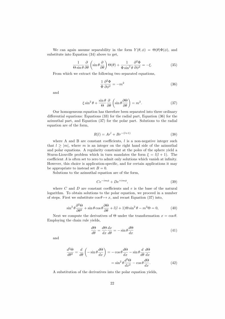
Figure 1: T2 axial fast spin echo image showing acute ischemia in the PCAdistribution. There is relative hyperintensity in the left occipital region of in-farction. Note the prominent hyperintensity of the vitreous and cerebrospinalfluid, both consistent with the hyperintensity of water on T2-weighted imaging.
Content Outline
The remainder of this paper is organized as follows: Section (2) presents anoverview of the MRI, Section (3) reviews the MRI assessment of acute ischemicstroke, Section (4) describes the hydrogen atom and reviews an analytical solu-tion to its Schrodinger equation, Section (5) reviews intrinsic spin, Section (6)reviews quantum mechanical addition of orbital angular momentum and spin,Section (7) reviews Group Theory of SU(2) and SO(3) and their relationship,and Section (8) summarizes this review.
The MRI section, Section (2), contains a number of subsections which areoutlined as follows: Subsection (2.1) discusses the hierarchy of scales in MRIphenomenology, Subsection (2.2) reviews the magnetism of electrons and nu-cleons, Subsection (2.3) reviews the magnetic potential energy and its role inthe descriptions of magnetization, torque, force, and larmor precession, Subsec-tion (2.4) reviews pulse magnetization, Subsection (2.5) describes equilibriummagnetization, Subsection (2.6) describes spin-lattice or T1 recovery, Subsec-tion (2.7) describes spin-spin or T2 decay, Subsection (2.8) reviews free induc-tance decay, Subsection (2.9) reviews the Bloch equations, Subsection (2.10)overviews intravenous contrast agents in MRI, Subsection (2.11) reviews gradient-based band-selection method for MRI space localization, and Subsection (2.12)reviews the components of the MRI machine.
The stroke section, Section (3), contains a number of subsections which are
2

outlined as follows: Subsection (3.1) reviews diffusion weighted imaging (DWI),Subsection (3.2) reviews perfusion weighted imaging (PWI), Subsection (3.3)reviews the combination of DWI and PWI and its utility in imaging the penum-bra, Subsection (3.4) reviews magnetic resonance spectroscopy, Subsection (3.5)reviews blood oxygen level dependent (BOLD) imaging, and Subsection (3.6)reviews MRA.
Appnedix (A) reviews the signals processing involved in MRI, including theFourier transforms, the canonical sampling theorem, and the convolution theo-rem.
2 Magnetic Resonance Imaging
The MRI is an optical technology whose core equation is the Maxwell-FaradayEquation. It exploits ensemble phenomena in which the composition of a samplecan be probed by sensing its magnetic properties through radio frequency waves.Here, we describe the various parts of MRI and their respective roles in thewhole.
2.1 A Hierarchy of Scales
The hierarchy of scales in the modeling of magnetic resonance imaging proceedsfrom the subnuclear scale of quarks and gluons, to the subatomic scale of discreteelectrons and nucleons, and finally to the bulk sample scale where ensembleeffects and statistical mechanics are the operative physics. In a general sense,the subnuclear scale is coupled to quantum field theory, the subatomic scale iscoupled to quantum mechanics, and the bulk sample scale is coupled to classicalelectromagnetics.
Certain phenomena in MRI are only meaningful over specific regimes. Forinstance, a magnetic moment experiences a torque when an external magneticfield is applied. However, the concept of torque is a classical concept. It isdeterministic and continuous, and is meaningful only at the level of ensemble orbulk effect. On the microscopic level, such as on the scale of single electrons andnucleons, quantum mechanics is the operative physics, and state transitions arequantized. This is encoded in the time evolution of quantum states governedby an appropriate Hamiltonian, yielding the specific Schrodinger equation thatapplies in that setting.
Although pedagogically separable, the scales are intrinsically linked physi-cally. For instance, the bulk magnetization, M, is the net sum of the atomiclevel magnetic moments, µj . Similarly the pulse magnetization frequency usedto torque the bulk magnetization vector and change its direction is a radio fre-quency wave, B1, oscillating at the larmor frequency of the individual nucleons.Furthermore, B1 takes its effect by acting directly on the individual electronsand nucleons, causing them to precess in phase.
2.2 Magnetism of Electrons and Nucleons
Electrons, protons, and neutrons are magnets. They derive their magnetismfrom intrinsic spin and orbital angular momentum. In the presence of an ex-ternally applied magnetic field, this results in bulk magnetism of sample tissue.
3

The magnetic dipole moment, µ, of a single unpaired electron or nucleon isgiven by,
µ = γS, (1)
where γ is the gyromagnetic ratio measured in Hz/T (Hertz per Tesla) andS is the spin. The gyromagnetic ratio for the electron is given by,
γe = gee
2me, (2)
where e is the elementary charge, me is the mass of the electron, and ge is theelectron gyromagnetic factor (g-factor), a dimensionless number whose experi-mental agreement with theory is near unprecedented on this scale, and therebylends strong credibility to the theory of quantum electrodynamics. Table (2)shows the electron and proton g-factors. The gyromagnetic ratio for nucleonsis given by,
γn = gpe
2mp, (3)
where mp is the mass of the proton, and gn is the g-factor of the nucleon.Estimated gyromagnetic ratios of some biologically-relevant nuclei are shown inTable (1) [13, 60].
Table 1: Gyromagnetic ratios of some biologically-relevant nuclei
Element Nuclei γn (106 rad s−1 T−1) γn/2π(MHz T−1)
Hydrogen 1H 267.513 42.576Deuterium D, 2H 41.065 6.536Helium 3He -203.789 -32.434Lithium 7Li 103.962 16.546Carbon 13C 67.262 10.705Nitrogen 14N 19.331 3.007Nitrogen 15N -27.116 -4.316Oxygen 17O -36.264 -5.772Fluorine 19F 251.662 40.053Nitrogen 14N 19.331 3.007Sodium 23Na 70.761 11.262Phosphorus 31P 108.291 17.235
The Bohr magneton, µB , and the nuclear magneton, µN , are named quan-tities related to the electron and proton gyromagnetic ratios respectively, andare given by,
µB =e~
2me, (4)
and
µN =e~
2mp. (5)
The magnetic moment of the electron is much larger than that of the nu-cleons, and as is discussed below, this corresponds to smaller precession, pulse,and signal frequency for protons than electrons. Specifically, nucleons precess,
4

absorb, and emit electromagnetic signals in the radio frequency range. Thisrange is non-ionizing radiation, and makes MRI a safer choice than ionizingimaging modalities such as plane and computed tomography X-rays.
Figure 2: T1 FLAIR. Sagittal section. Note the hyperintensity of orbital fat,and the hypointensity of vitreous and cerebrospinal fluid. Hyperintensity of fatand hypointensity of water are radiologic characteristics of T1 weighted imaging.
2.3 The Magnetic Potential Energy
The magnetic potential energy is,
U = −µ ·B. (6)
The force on a magnetic moment, the torque on a magnetic moment, andthe larmor precession frequency or resonance frequency, can all be described interms of the magnetic potential energy, U(r, t).
2.3.1 Magnetization
The magnetic moment aligns itself in either parallel or anti-parallel orientationto the external field B0. The extent of parallelism is constrained by the eigenval-ues of the S2 and Sz operators above, such that from the geometry, the paralleland anti-parallel states make angles of cos−1(1/
√3) ≈ 54.7356103172 degrees
with the positive and negative z-axes respectively (assuming B0 is oriented ex-clusively along the z-axis).
This process is called magnetization. In the case of a population sample,upon application of B0, the spin orientation distribution goes from a somewhatarbitrary array of directions to being composed of only two directions, paralleland antiparallel. The parallel orientation is the lower energy state, and therebyis the more populous state for protons in the sample. The population distri-bution is temperature dependent, such that the proportion of protons in thehigher energy state increases with temperature. The relationship is given by,
5

NhNl
= e−E/kT , (7)
where Nh is the higher energy state, Nl is the lower energy state, E is theenergy difference between the two states, k is the Boltzmann constant, and Tis the absolute temperature in Kelvin. The bulk magnetization can be modeledas,
M(t) =∑j
µj(t). (8)
with B0 = zB0, it follows that M(0) = Mz(0) and Mxy = 0. In other words,the equilibrium magnetization is entirely along the z (longitudinal) directionand there is no component in the xy (transverse) direction.
2.3.2 Torque
The torque on a magnetic moment in a magnetic field acts to align it with thefield, is a function of the magnetic potential energy, and is given by,
τ(α) = − ∂
∂α(−µ ·B), (9)
where α is the angle between B and µ, and the minus sign indicates therestoring nature of the torque.
2.3.3 Force
The force on a nucleon or electron in a magnetic field is,
F = −∇(−µ ·B). (10)
2.3.4 Precession
When an external magnetic field B0 is applied to an electron or neutron par-ticle, the particle’s magnetic moment precesses about the direction of B0at afrequency called the larmor frequency given by,
ω = γB0. (11)
In the equilibrium magnetization state with B0 = zB0 and Mxy = 0, thereis no precession of the bulk magnetization M because µ = M×B0 = 0.
Considering only the spin of a spin 1/2 object in a magnetic field, andassuming B = ez, we get the following Hamiltonian,
H = −µ ·B = −(−gxe2mx
S) ·B := ω · S, (12)
where the subscript x denotes either e for electron or p for a neutron, andwhere,
ω :=gxeB
2meez. (13)
It follows that,
6
H = ωSz. (14)
We see that remarkably, the Hamiltonian is proportional to the z-componentof spin, therefore the magnetic spin eigenstates are simultaneously energy eigen-states. Furthermore the energy eigenvalues are proportional to the magneticspin quantum numbers. Specifically,
E± = ±1
2~ω. (15)
The above relation led early researchers to the discovery of spin, by itsmanifestation as the Zeeman effect and the splitting of energy levels in thehydrogen optical spectrum.
2.4 Pulse Magnetization
Given a bulk magnetization M due to a static magnetic field B0 = B0z, apulse of a weaker magnetic field, B1, oscillating at the larmor frequency andapplied perpendicular to B0, will result in a transition of the individual nucleonsfrom dephased to in-phase oscillation. This manifests as the acquisition of atransverse phase Mxy and oscillations of M about the z-axis at the larmorfrequency ω. This “tilting” of the magnetization vector also implies a decreasein Mz. During the pulse, the net external magnetic field is the sum of B0
and B1. If the pulse duration was extended indefinitely, the result would bealignment of the bulk magnetization with the new direction, B0 +B1, and therewould be no resultant oscillation observed. The pulsed nature of B1 is thereforecritical to the technology of magnetic resonance imaging.
2.5 Equilibrium Magnetization
The net magnetization is given by,
M = (Nl −Nh)µ, (16)
while the ratio of Nl to Nh is given in Equation (7) above as, Nh
Nl= e−E/kT .
At equilibrium, the solution of the above system of two equations yields theequilibrium magnetization,
M0 =B0γ
2~2
4k-Tρp, (17)
where k- = k/2π is the reduced Boltzmann constant and ρp is the protondensity.
2.6 Spin-Lattice Relaxation (T1 Relaxation)
The spin-lattice relaxation, also known as T1 relaxation or longitudinal relax-ation, is the process of longitudinal magnetization recovery following a B1 per-turbation. Specifically, T1 is the time constant of longitudinal magnetizationrecovery, and is given by,
Mz(t) = M0(1− e−t/T1) +Mz(0)e−t/T1, (18)
7

where M0 is equilibrium magnetization and Mz(0) is the longitudinal magne-tization instantaneously after pulse excitation. In inversion recovery, the initialmagnetization is negative, and typically Mz(0) = −M0. Substituting this valueinto Equation (18) above yields,
Mz(t) = M0(1− 2e−t/T1). (19)
Fluid attenuated inversion recovery (FLAIR) is useful in the diagnosis ofcertain pathologies such as periventricular white-matter lesion in multiple scle-rosis. FLAIR can be T1 or T2 weighted. Figure (2) shows a sagittal section ofa T1 FLAIR brain image, and Figure (3) shows a T2 FLAIR brain image.
Figure 3: T2 FLAIR showing hyperintense signal in the PCA and MCA distri-butions, consistent with acute ischemic stroke. Note that the hypointensity ofcerebrospinal fluid due to fluid-attenuation allows for better contrast with theperiventricular lesion.
2.7 Spin-Spin Relaxation (T2 Relaxation)
The spin-spin relaxation, also known as T2 relaxation or transverse relaxation, isthe process of transverse magnetization relaxation following a B1 perturbation.Specifically, T2 is the time constant of transverse magnetization recovery, andis given by,
Mxy(t) = Mxy(0)e−t/T2, (20)
8

where Mxy(0) is the transverse magnetization instantaneously after pulseexcitation. Following the B1 induction of in-phase precession, the proton spinsagain begin to dephase according to T2 time constant. Of note, the relaxationof transverse magnetization is faster than the recovery of longitudinal magneti-zation. In other terms, T2 < T1. Figure (1) shows a T2 fast spin echo image ofacute ischemic stroke in the posterior circulation.
2.8 Free Inductance Decay
Upon pulse excitation and tilting, the magnetization vector oscillates about thez-axis. This oscillating magnetic moment in turn generates an electromotiveforce in accordance with Faraday-Maxwell law of electromagnetic induction,
∇×E = −∂B∂t, (21)
where ∇× is the curl operator, E(r, t) is the electric field, and B(r, t) is themagnetic field. The above equation can be rendered in integral form via Stokestheorem to yield, ∮
∂Σ
E · ds = − ∂
∂t
∫∫Σ
B · dA, (22)
where ∂Σ can represent a wire coil bounding a surface Σ, ds is an infinitesi-mal segment length along the wire, and dA is vector normal to an infinitesimalarea of Σ. Such integral transformation has certain advantages in numericalcomputation. For instance, Green’s functions approaches can be invoked andcan greatly decrease the number of unknowns, thereby decreasing the compu-tational resource demand of the problem.
The radio frequency (RF) coils within the MRI probe experience an elec-tromotive force due to the rotating magnetization. This results in an electriccurrent signal which is fed as output to a screen. The signal decays with timeaccording to the T2 time constant, hence the name Free Inductance Decay (FID)signal [101].
2.9 Bloch Equations
The Bloch equations describe the time evolution of the bulk magnetizationvector, and are therefore also referred to as the equations of motion of magne-tization. They are given by,
∂Mx(t)
∂t= γ(M(t)×B(t))x −
Mx(t)
T2, (23)
∂My(t)
∂t= γ(M(t)×B(t))y −
My(t)
T2, (24)
and∂Mz(t)
∂t= γ(M(t)×B(t))z −
Mz(t)−M0
T1, (25)
where γ is the gyromagnetic ratio of the nucleon and B(t) = B0 + B1(t)
9

2.10 Intravenous MR Contrast Agents
There are several contrast agents in current clinical use, most of which arebased either on low molecular weight chelates of gadolinium ion (Gd3+) [23, 16]such as Gadolinium-DPTA, or are based on iron oxide (FeO) such as Fe3O4,Fe2O3, and γ-Fe2O3 (or gamma phase maghemite) [17, 4, 59, 49]. Based ontheir magnetic properties, they confer contrast of vasculature from background,and by proxy of vascularization density, of organs from surround. Specifically,the Gd3+-based agents predominantly shorten T1 time, while the FeO-basedagents predominantly shorten T2 time. Nanoparticle formulations of contrastagents are in various stages of development and can be based on gadoliniumor iron-oxide, or on other agents such as cobalt, nickel, manganese, or cop-per ions [109, 56, 4]. Optimization of the efficacy of MR contrast agents is anactive area of research [21, 50, 53, 92, 72, 48, 54]. The growing array of MRcontrast applications has included efforts to target tissue or tumor-specific recep-tors [54, 61, 22, 112, 36, 76, 103]. Serious adverse reactions to intravenous MRIcontrast agents are rare. However in the mid 2000s gadolinium chelates were in-creasingly hypothesized as playing a role in nephrogenic systemic fibrosis (NSF),a disease entity unknown prior to 1997. It has since been essentially establishedthat Gadodiamide, a gadolinium-containing agent, is associated with an in-creased risk of developing NSF in susceptible individuals [12, 55, 97, 106, 68].Superparamagnetic iron oxides have been promoted by some as possible alter-natives to gadolinium-based agents in patients at risk for NSF [81].
2.11 Gradient-based 3D Spatial Localization
For 3D localization, a gradient coil generates a magnetic field gradient in thebore. Then in accordance with the larmor frequency relation ω = γB(r, t), itfollows that the resonance frequency, ω = ω(r, t) acquires space dependence,and thereby serves to effectively label the tissue in space. The process of space-specific excitation of the sample is called slice selection. The excitation pulsefrequency is simply chosen as a bandwidth frequency flanking the region-of-interest or the slice. The process of scanning is an iteration, however simpleor complex, through a sequence of slices. And slice thickness is proportional toexcitation pulse bandwidth. The slice thickness can be decreased by decreasingthe bandwidth, or alternatively by increasing the magnetic field gradient. Forinstance, given a constant magnetic field gradient, the slice thickness betweentwo points r1 and r2 is given by,
ω(r2)− ω(r1)
γ[B(r2)−B(r1)]= r2 − r1 (26)
Both the bandwidth and magnetic field gradient are Graphical User Interface(GUI)- adjustable parameters on current day MRI machines. This gradient-based localization technique was Paul Lauterbur’s contribution to the develop-ment of MRI [58].
2.12 MRI Machinery
The MRI is a simple machine in principle. It was was invented by Raymond V.Damadian by 1971 [30, 32, 31, 111]. It consists of a magnet, a radio frequency
10

coil, an empty space or bore, and a computer processor. The magnet is forapplying the static and pulsed magnetic fields. Current day machines typicallyuse superconducting electromagnets. These are wire coils cooled to low temper-atures using liquid helium and liquid nitrogen [29, 63, 14, 47, 44, 107, 71, 111],allowing for greatly decreased electrical resistance, and consequently high cur-rent loops generating strong magnetic fields. The RF coil typically serves bothas the generator of the pulsed magnetic field, and as the detector of the FIDsignal. Such duality of function is possible simply because the Maxwell-Faradayequation is true in both directions. Several machines also have a separate gra-dient coil. The gradient coil has x, y, and z components indicating the spatialdirection of the gradient field, and together conferring 3D localization. The com-puter processor runs the software instructions for pulse sequences and signalsprocessing, including image reconstruction.
2.12.1 Superconductivity
MRI requires strong magnetic fields. Though the Earth’s magnetic field isvariable with time and is asymmetric between northern and southern hemi-spheres [85], it is estimated to range between 25,000 and 65,000 nanoteslas (0.25to 0.65 Gauss) at the surface, with a commonly cited average of 46,000 nanotesla(0.46 Gauss) [113]. Current clinical use MRIs commonly range from 1.5 Teslato 7 Teslas. Therefore MRIs may require magnetic fields up to 280,000 timesthe earth’s magnetic field. This has been achieved by a shift from permanentmagnets to superconducting electromagnets, and presents another interdisci-plinary link to both theory and practice. The dominant physical theory of su-perconductivity is called BCS theory [7, 25, 8, 9] after its formulators, Bardeen,Cooper, and Schrieffer, and is based on electron pairing via phonon-exchangeto form so called Cooper pairs. Though electrons are fermions and subjectto the Fermi exclusion principle, precluding any two electrons occupying thesame state, Cooper pairs act like bosons because their pairing and spin summa-tion results in integer-spin character, a type of boson-like state. Upon cooling,these boson-like pairs can condense, analogous to Bose-Einstein condensationand representing a quantum phase transition. Quantum phase transitions havehistorically been challenging to study in a controlled way in the laboratory, buthave recently been demonstrated by H. T. Mebrahtu et. al. in tunable quantumtunnelling studies of Luttinger liquids [70]. In superconductivity, upon transi-tion into the condensed state, the coherence of the system imposes a high energypenalty on resistance, effectively resulting in a zero resistance state. This is for-mally encoded in the theory by an energy gap at low (subcritical) temperatures.In superconducting electromagnets, the coil cooling is done through liquid he-lium and liquid nitrogen and presents a connection to the chemistry of phasetransitions, condensed matter and solid state physics, as well as the engineeringaspects of attaining and maintaining such low temperatures.
3 MRI Assessment of Acute Ischemic Stroke
In this section, we review the MRI modalities used in the assessment of acuteischemic stroke.
11
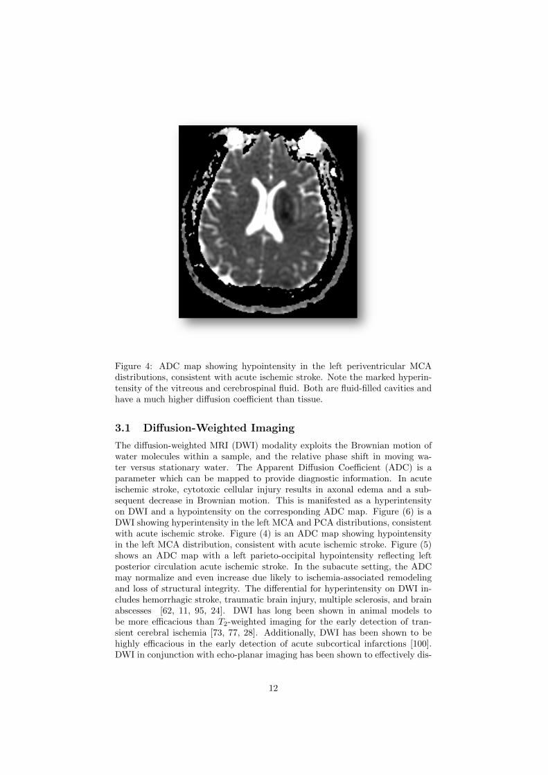
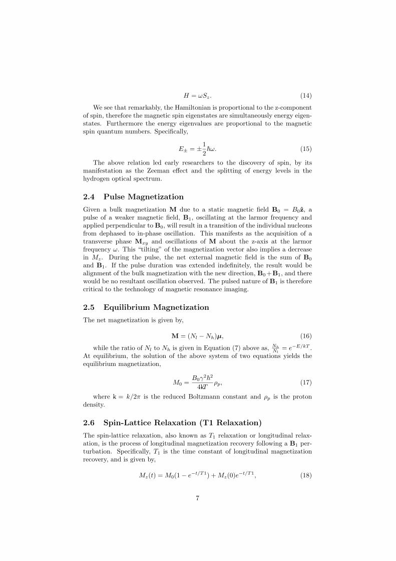
Figure 4: ADC map showing hypointensity in the left periventricular MCAdistributions, consistent with acute ischemic stroke. Note the marked hyperin-tensity of the vitreous and cerebrospinal fluid. Both are fluid-filled cavities andhave a much higher diffusion coefficient than tissue.
3.1 Diffusion-Weighted Imaging
The diffusion-weighted MRI (DWI) modality exploits the Brownian motion ofwater molecules within a sample, and the relative phase shift in moving wa-ter versus stationary water. The Apparent Diffusion Coefficient (ADC) is aparameter which can be mapped to provide diagnostic information. In acuteischemic stroke, cytotoxic cellular injury results in axonal edema and a sub-sequent decrease in Brownian motion. This is manifested as a hyperintensityon DWI and a hypointensity on the corresponding ADC map. Figure (6) is aDWI showing hyperintensity in the left MCA and PCA distributions, consistentwith acute ischemic stroke. Figure (4) is an ADC map showing hypointensityin the left MCA distribution, consistent with acute ischemic stroke. Figure (5)shows an ADC map with a left parieto-occipital hypointensity reflecting leftposterior circulation acute ischemic stroke. In the subacute setting, the ADCmay normalize and even increase due likely to ischemia-associated remodelingand loss of structural integrity. The differential for hyperintensity on DWI in-cludes hemorrhagic stroke, traumatic brain injury, multiple sclerosis, and brainabscesses [62, 11, 95, 24]. DWI has long been shown in animal models tobe more efficacious than T2-weighted imaging for the early detection of tran-sient cerebral ischemia [73, 77, 28]. Additionally, DWI has been shown to behighly efficacious in the early detection of acute subcortical infarctions [100].DWI in conjunction with echo-planar imaging has been shown to effectively dis-
12

Figure 5: ADC map showing hypointensity in the PCA distribution, consistentwith a parieto-occipital acute ischemic stroke
criminate between high grade (high cellularity) and low grade (low cellularity)gliomas [104]. Of note, in spite of the relatively high specificity and sensitivityof DWI in the early detection of acute ischemic stroke, there is a small subset ofstroke patients who evade DWI detection in spite of clinically evident stroke-likeneurological deficits [2]. DWI tractography or diffusion tensor imaging is a formof principal component analysis in which the dominant eigendirection is used todetermine the path of an axonal tract in a given voxel. This method has shownpotential for further elucidation of neuronal pathways in the brain.
3.2 Perfusion-Weighted Imaging
Perfusion-weighted imaging (PWI) is an ordinary differential equations com-partment model of blood perfusion through organs. An arterial input function(AIF) is determined as input into the particular chosen model. The AIF isan impulse, and the model is essentially described by an impulse response orGreen’s function. The computed output are perfusion parameters such as meantransit time, time to peak, cerebral blood flow rate, and cerebral blood vol-ume. There are various protocols for the perfusion conditions. For instancethe dynamic susceptibility contrast imaging method uses gadolinium contrastto gather local changes in T2∗ signal in surrounding tissue. T2∗ is a type of T2 inwhich static dephasing effects are not explicitly RF-canceled, therefore dephas-ing from magnetic field inhomogeneities and susceptibility effects contribute toa tighter FID envelope (more rapid decay; T2∗ < T2) than is seen in T2. Other
13

Figure 6: DWI showing hyperintensity in the left PCA and MCA distributions,consistent with acute ischemic stroke.
PWI protocols include arterial spin labeling and blood oxygen level dependentlabeling. Not surprisingly, PWI results vary with the choice of perfusion modeland computational method with which it is implemented [116, 105, 39, 89].
3.3 Combined Diffusion and Perfusion-Weighted Imaging
Both PWI and DWI are efficacious in the early detection of cerebral ischemiaand correlate well with various stroke quantitation scales [108, 6, 93]. Further-more, the combination of diffusion and perfusion-weighted imaging allows forassessment of the ischemic penumbra, that watershed region at the boundary ofinfarcted and non-infarcted tissue [80, 99, 115, 98]. It represents tissue which hassuffered some degree of ischemia, but remains viable and possibly salvageableby expedient intervention with thrombolytic therapy [69, 88, 18], hypothermia,blood pressure elevation, or other experimental methods under study. Outsidethe penumbra, thrombosis or autoregulation of circulation shuts down perfu-sion to infarcted tissue, resulting in a drastic decrease in perfusion. Diffusion issimultaneously decreased due to tissue ischemia, hence no PWI-DWI mismatchoccurs. Within the penumbra however, the tissue is hypoperfused, yet sincestill viable, it has yet to sustain sufficient cytotoxic axonal damage to manifesta significant decrease in diffusion. The registration of both imaging modali-ties therefore demonstrates a diffusion-perfusion mismatch at the penumbra.In set-theoretic terms, the brain territory ∆ with compromised diffusion is a
14

proper subset of the territory Ψ with compromised perfusion, and the relativecomplement of ∆ in Ψ is called the ischemic penumbra Λ,
Λ = ∆c ∩ Ψ = Ψ \∆ (27)
One caveat to PWI-DWI mismatch assessment is that when done subjec-tively by the human eye, it can be demonstrably unreliable [26]. Hence devel-opment of quantitative metrics and learning algorithms are needed in this area.For instance, generalized linear models have been used and shown promise [115].
Figure 7: 3D time-of-flight image of the carotid vasculature. Axial section ofneck shown.
3.4 Magnetic Resonance Spectroscopy
Magnetic resonance spectroscopy (MRS) is being used in attempts to reliablymeasure the magnetic resonance of metabolites whose concentrations changein the setting of acute ischemic stroke. Lactate (LAC) levels are well knownto increase in ischemia, and is therefore a candidate in development, while N-acetyl aspartate (NAA) levels have been shown to decrease in acute stroke, andare used in proton spectroscopy studies. Most studies confirming the ischemia-associated elevation in LAC and decrease in NAA have been done in the settingof hypoxic-ischemic encephalopathy in newborns [20, 10, 67]. In addition tolactate, α-Glx and glycine have also been shown to be increased in the as-phyxiated neonate [64]. Phosphorus magnetic resonance spectroscopy detects
15

Figure 8: 2D time-of-flight fast spoiled gradient echo sequence (FSPGR) imageof the carotids.
changes in the resonance spectrum of energy metabolites, and has also shownprognostic significance in hypoxic-ischemic brain injury [3, 90]. In their currentform, MRS methods are less sensitive and practical for the assessment of acuteischemic stroke than the other magnetic resonance modalities discussed here.However, MRS is rapidly finding a place in the routine clinical assessment ofhypoxic-ischemic encephalopathy in the asphyxiated neonate. Some neonatalintensive care units, for instance, now conduct MRS studies on all neonatesbelow a certain threshold weight.
3.5 Blood Oxygen Level-Dependent (BOLD) MRI
The blood oxygen level-dependent (BOLD) MRI is a magnetic resonance imag-ing method that derives contrast from the difference in magnetic propertiesof oxygenated versus deoxygenated blood. Hemoglobin is the molecule whichcarries oxygen in the blood, and is located in red blood cells. The oxygen-bound form of hemoglobin is called oxyhemoglobin, while the oxygen-free formis called deoxyhemoglobin. Deoxyhemoglobin is paramagnetic and in the pres-ence of an applied magnetic field assumes a relatively higher magnetic dipolemoment than oxyhemoglobin which is a diamagnetic molecule. Deoxygenatedblood has a higher concentration of deoxyhemoglobin than oxyhemoglobin, andthis difference is reflected in the MRI signal. T2∗-based BOLD MRI has shownpromise in localizing the penumbra in acute ischemic stroke [42, 38]. It is alsoused in functional MRI (fMRI), which is based on the principle that active brainareas have higher resource (e.g. oxygen, glucose) demands and higher waste out-put [43]. In this context, BOLD has been used to study the brain’s behaviorduring sensorimotor recovery following acute ischemic stroke. Specifically, thecoupling between BOLD and electrical neuroactivity has shed some light onthe still poorly understood process of spontaneous motor recovery following a
16

Figure 9: MRA showing axial view of the internal carotids and Circle-of-Willis
stroke [15, 19, 52, 94, 27]. BOLD MRI results can be affected by baseline cir-culatory status, and therefore in the research setting near-infrared spectroscopy(NIRS) can be used as a control, or as an alternative modality in the clinic[102, 78]. BOLD MRI has been used in assessing the brain’s response to hyper-capnia [110, 5]. Hypercapnia can cause changes in multiple variables in the brainsuch as cerebral blood flow, oxygen consumption rate, cerebral blood volume,arterial oxygen concentration, and red blood cell volume fraction. However,hypercapnia-associated cerebrovascular reactivity has been strongly correlatedwith arterial spin labeling and other PWI surrogates, suggesting that the brain’sreaction to hypercapnia is dominated by changes in cerebral blood flow [66].
3.6 Magnetic Resonance Angiography
MRA is a set of magnetic resonance-based techniques for imaging the circulatorysystem. Figures (9) and (10) show MRA images of the Circle-of-Willis. MRAtechniques can be broadly categorized into flow-dependent and flow-independentgroups. The flow-dependent methods derive contrast from the motion of bloodin vasculature relative to the static state of surrounding tissue [33]. Two cur-rently well-known and used examples of flow dependent methods are: (i) Phasecontrast MRA, (PC MRA) [34, 37, 91] and (ii) Time-of-Flight MRA (TOFMRA). The TOF MRA images can be acquired in either two dimensional (2DTOF) or three dimensional (3D TOF) formats. Figure (8) shows a 2D TOF fastspoiled gradient echo sequence (FSGR) image of the carotids, and Figure (7)shows a an axial section of a 3D TOF image of the carotids. PC MRA exploitsdifferences in spin phase of moving blood relative to static surrounding tissue,while TOF MRA exploits the difference in excitation pulse (B1) exposure of
17
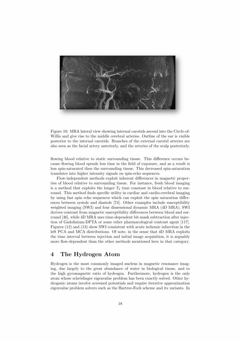
Figure 10: MRA lateral view showing internal carotids ascend into the Circle-of-Willis and give rise to the middle cerebral arteries. Outline of the ear is visibleposterior to the internal carotids. Branches of the external carotid arteries arealso seen as the facial artery anteriorly, and the arteries of the scalp posteriorly.
flowing blood relative to static surrounding tissue. This difference occurs be-cause flowing blood spends less time in the field of exposure, and as a result isless spin-saturated then the surrounding tissue. This decreased spin-saturationtranslates into higher intensity signals on spin-echo sequences.
Flow-independent methods exploit inherent differences in magnetic proper-ties of blood relative to surrounding tissue. For instance, fresh blood imagingis a method that exploits the longer T2 time constant in blood relative to sur-round. This method finds specific utility in cardiac and cardio-cerebral imagingby using fast spin echo sequences which can exploit the spin saturation differ-ences between systole and diastole [74]. Other examples include susceptibilityweighted imaging (SWI) and four dimensional dynamic MRA (4D MRA). SWIderives contrast from magnetic susceptibility differences between blood and sur-round [46], while 4D MRA uses time-dependent bit-mask subtraction after injec-tion of Gadolinium-DPTA or some other pharmacological contrast agent [117].Figures (12) and (13) show SWI consistent with acute ischemic infarction in theleft PCA and MCA distributions. Of note, in the sense that 4D MRA exploitsthe time interval between injection and initial image acquisition, it is arguablymore flow-dependent than the other methods mentioned here in that category.
4 The Hydrogen Atom
Hydrogen is the most commonly imaged nucleus in magnetic resonance imag-ing, due largely to the great abundance of water in biological tissue, and tothe high gyromagnetic ratio of hydrogen. Furthermore, hydrogen is the onlyatom whose schrodinger eigenvalue problem has been exactly solved. Other hy-drogenic atoms involve screened potentials and require iterative approximationeigenvalue problem solvers such as the Hartree-Fock scheme and its variants. In
18

Figure 11: MRA of the neck showing the carotid vasculature.
what follows we review the electronic orbital configuration of hydrogen.
4.1 Electronic Orbital Configuration
In this section we focus on the electron. Specifically that lone electron in theorbit of the hydrogen atom. We make this choice because its simplicity allowsus review the attributes of quantum orbital angular momentum and spin, in acontext which is not only real, but also highly relevant to magnetic resonanceimaging, which as noted targets the hydrogen atom. The electron in 1H has bothposition and angular momentum. The Hamiltonian commutes with the squaredorbital angular momentum operator, therefore angular momentum eigenstatesare also energy eigenstates. Of note, the position and angular momentum ob-servables do not commute. This is equivalent to Heisenberg’s uncertainty princi-ple. Hence definite energy or orbital angular momentum states, are representedin the position basis as probability density functions, which are synonymouswith electron clouds or atomic orbitals.
Orbital angular momentum is the momentum possessed by a body by virtueof circular motion, as along an orbit. In quantum mechanics, the square ofthe orbital momentum is a quantized quantity, which can take on only certaindiscrete “allowed” values. This reality and discreteness of the orbital momen-tum eigenvalues is a manifestation of the spectral theorem of normal boundedoperators; given the hermiticity and boundedness of the quantum orbital angu-lar momentum operator over a specified finite volume such as the radius of anatom; which is itself a manifestation of the negative energy of the electron inorbit yielding a so called bound state. The orbital momentum states can be indi-rectly represented by the spherical harmonic functions to be derived below. Thespherical harmonics are the eigenfunctions of the squared quantum orbital angu-lar momentum operator in spherical coordinates. Their product with the radialwave functions yield the wave function, ψ, of the hydrogen’s electron. Where
19
Figure 12: SWI showing signal in the left MCA distribution consistent withacute ischemic infarct. Note the left periventricular region of hyperintensity.Its hypointense center is consistent with the ischemic core.
in accordance with the principal postulate of quantum mechanics, ψ2(r, θ, φ) isthe probability of finding the electron at a given point (r, θ, φ).
In the time-independent case, the Hamiltonian defines the Schrodinger equa-tion as follows,
Hψ = Eψ. (28)
The orbital angular momentum states are the angular portion of the solu-tion, ψ, of the schrodinger equation in spherical coordinates. Substituting theexpression for the Hamiltonian of a single non-relativistic particle into Equa-tion (28) yields,
− ~2
2m∇2ψ(r) + V (r)ψ(r) = Eψ(r), (29)
where r ∈ <3. In spherical coordinates the above equation becomes,
− ~2r−2
2m sin θ
[sin θ
∂
∂r
(r2 ∂
∂r
)+
∂
∂θ
(sin θ
∂
∂θ
)+
1
sin θ
∂2
∂φ2
]ψ(r)
+V (r)ψ(r) = Eψ(r), (30)
where m denotes mass. Invoking the method of separation of variables, weassume existence of a solution of the form ψ(r) = R(r)Y (θ, φ). We illustrate
20

Figure 13: SWI showing signal in the left PCA and MCA distributions consis-tent with acute ischemic infarct. Note the bull’s eye pattern of hyperintensitysurrounding some central foci of hypointensity in the occipital lesion.
the method on the Laplace equation which can be interpreted as a homogeneousform of the schrodinger equation, i.e. one for which V (r) = E = 0,
Y
r2
∂
∂r
(r2 ∂
∂r
)R(r) +
R
r2 sin θ
∂
∂θ
(sin θ
∂
∂θ
)Y (θ, φ) +
R
r2 sin2 θ
∂2Y
∂φ2
= 0. (31)
Multiplying through by r2/RY yields,
1
R
∂
∂r
(r2 ∂
∂r
)R(r) +
1
Y sin θ
∂
∂θ
(sin θ
∂
∂θ
)Y (θ, φ) +
1
Y sin2 θ
∂2Y
∂φ2
= 0, (32)
which can be separated as,
1
R
∂
∂r
(r2 ∂
∂r
)R(r) = ξ (33)
and
1
Y sin θ
∂
∂θ
(sin θ
∂
∂θ
)Y (θ, φ) +
1
Y sin2 θ
∂2Y
∂φ2= −ξ. (34)
21
We can again assume separability in the form Y (θ, φ) = Θ(θ)Φ(φ), andsubstitute into Equation (34) above to get,
1
Θ sin θ
∂
∂θ
(sin θ
∂
∂θ
)Θ(θ) +
1
Φ sin2 θ
∂2Φ
∂φ2= −ξ. (35)
From which we extract the following two separated equations,
1
Φ
∂2Φ
∂φ2= −m2 (36)
and
ξ sin2 θ +sin θ
Θ
∂
∂θ
(sin θ
∂Θ
∂θ
)= m2. (37)
Our homogeneous equation has therefore been separated into three ordinarydifferential equations: Equations (33) for the radial part, Equation (36) for theazimuthal part, and Equation (37) for the polar part. Solutions to the radialequation are of the form,
R(l) = Arl +Br−(l+1) (38)
where A and B are constant coefficients, l is a non-negative integer suchthat l ≥ |m|, where m is an integer on the right hand side of the azimuthaland polar equations. A regularity constraint at the poles of the sphere yield aSturm-Liouville problem which in turn mandates the form ξ = l(l + 1). Thecoefficient A is often set to zero to admit only solutions which vanish at infinity.However, this choice is application-specific, and for certain applications it maybe appropriate to instead set B = 0.
Solutions to the azimuthal equation are of the form,
Ce−imφ +De+imφ, (39)
where C and D are constant coefficients and e is the base of the naturallogarithm. To obtain solutions to the polar equation, we proceed in a numberof steps. First we substitute cos θ 7→ x, and recast Equation (37) into,
sin2 θ∂2Θ
∂θ2+ sin θ cos θ
∂Θ
∂θ+ l(l + 1)Θ sin2 θ −m2Θ = 0, (40)
Next we compute the derivatives of Θ under the transformation x = cos θ.Employing the chain rule yields,
dΘ
dθ=dΘ
dx
dx
dθ= − sin θ
dΘ
dx(41)
and
d2Θ
dθ2=
d
dθ
(− sin θ
dΘ
dx
)= − cos θ
dΘ
dx− sin θ
d
dθ
dΘ
dx
= sin2 θd2Θ
dx2− cos θ
dΘ
dx. (42)
A substitution of the derivatives into the polar equation yields,
22

sin2 θ
(sin2 θ
d2Θ
dx2− cos θ
dΘ
dx
)+ sin θ cos θ
(− sin θ
dΘ
dx
)+l(l + 1)Θ sin2 θ −m2Θ = 0. (43)
Dividing through by sin2 θ and changing variables via cos θ 7→ x and Θ 7→ y,yields the associated (m 6= 0) Legendre differential equation,
(1− x2)∂2y
∂x2− 2x
∂y
∂x+
(l(l + 1)− m2
1− x2
)y = 0, (44)
whose solutions are given by
Pml (x) =(−1)m
2ll!(1− x2)m/2
dl+m
dxl+m(x2 − 1)l. (45)
The solution Y (φ, θ) = Φ(φ)Θ(θ) to angular portion of the Laplace equationis therefore of the form,
Yl,m(θ, φ) = NPml (cos θ)eimφ, (46)
where N is a normalization factor given by,
N =
√(2l + 1)
4π
(l − 1)!
(l + 1)!, (47)
and enabling, ∫Ω
Y ∗l,m(Ω)Yl,m(Ω) = 1, (48)
where Ω = (φ, θ) is solid angle. Yl,m are called the spherical harmonicfunctions and are discussed some more in the following subsection. Figures (14)to (23) are plots of a sampling of spherical harmonics with 1 ≤ l ≤ 5.
For the electronic configuration of the hydrogen atom, the electron experi-ences a potential V(r) due to the proton. V(r) is the coulomb potential givenby,
V (r) = − e2
4πε0r(49)
Substituting this into the generic schrodinger equation yields,
− ~2
2m∇2ψ(r)− e2
4πε0rψ(r) = Eψ(r), (50)
which in spherical coordinates is,
− ~2r−2
2m sin θ
[sin θ
∂
∂r
(r2 ∂
∂r
)+
∂
∂θ
(sin θ
∂
∂θ
)+
1
sin θ
∂2
∂φ2
]ψ(r)
− e2
4πε0rψ(r) = Eψ(r), (51)
where m is given by,
23

Figure 14: l=1,m=1
m =mpme
mp +me, (52)
and is the two-body reduced mass mp of the proton and me of the electron.Equation (51) above is an eigenvalue problem which after some rearranging,
we can solve using the same separation of variables method illustrated above.We recast as,
[∂
∂r
(r2 ∂
∂r
)+
2m
~2
(re2
4πε0+ Er2
)]R(r)Y (θ, ψ)
+
[1
sin θ
∂
∂θ
(sin θ
∂
∂θ
)+
1
sin2 θ
∂2
∂φ2
]R(r)Y (θ, ψ)
= 0 (53)
Dividing through by R(r)Y (θ, φ) and splitting the operator, we get,
1
Y (Ω)
[1
sin θ
∂
∂θ
(sin θ
∂
∂θ
)+
1
sin2 θ
∂2
∂φ2
]Y (Ω) = −l(l + 1) (54)
and
1
R(r)
∂
∂r
(r2 ∂
∂r
)R(r) +
2m
~2
[re2
4πε0+ Er2
]= l(l + 1). (55)
Equation (54) is exactly the same as Equation (35) which we solved above,and whose solutions are the spherical harmonic functions, Yl,m. Equation (55)above is isomorphic to a generalized Laguerre differential equation, whose so-lutions are related to the associated Laguerre polynomials. As mentioned inthe case of Laplace’s equation above, regularity conditions at the boundary
24

Figure 15: l=2,m=1
prescribe the separation constant l(l + 1). To transform Equation (55) into ageneralized Laguerre equation, we recast into the following form,
∂
∂r
(r2 ∂
∂r
)R(r) +
[2mre2
4πε0~2+
2mEr2
~2− l(l + 1)
]R(r) = 0. (56)
then we proceed with the following sequence of substitutions:
R(r) 7→ y(r)
r
−2mE
~27→ β2
4
r 7→ x
β. (57)
Executing the first substitution above transforms Equation (56) into,
d2y(r)
dr2+
[2me2
4πrε0~2+
2mE
~2− l(l + 1)
r2
]y(r) = 0. (58)
Next, the second substitution transforms the above into,
d2y(r)
dr2+
[2me2
4πrε0~2− β2
4− l(l + 1)
r2
]y(r) = 0. (59)
And finally, the third substitution transforms the above into,
β2 d2y(x)
dx2+
[2βme2
4πxε0~2− β2
4− β2l(l + 1)
x2
]y(x) = 0. (60)
Dividing through by β2 yields,
d2y(x)
dx2+
[−1
4+
2me2
4πβε0~2x− l(l + 1)
x2
]y(x) = 0. (61)
25

Figure 16: l=3,m=1
Next, we make the substitutions,
l(l + 1) 7→ k2 − 1
4(62)
and
2me2
4πβε0~27→ 2j + k + 1
2, (63)
which transform Equation (61) into the following generalized Laguerre equa-tion
(ykj )′′(x) +
[−1
4+
2j + k + 1
2x− k2 − 1
4x2
]ykj (x) = 0, (64)
whose solutions are readily verified to be the following associated Laguerrefunctions,
ykj (x) = e−x/2x(k+1)/2Lkj (x), (65)
where Lkj are the associated Laguerre polynomials.From Equation (62) we see that,
k = 2l + 1, (66)
which we substitute into Equation (63) to yield,
2me2
4πβε0~2=
2j + (2l + 1) + 1
2= j + l + 1 ≡ n. (67)
n is the principal (or radial) quantum number. The corresponding energyeigenvalues, En, are obtained by substituting β2 into n2 and solving for E, weget,
26

Figure 17: l=3,m=2
En = − ~2
2ma20n
2, (68)
where a0 is the Bohr radius and is given by,
a0 =4πε0~2
mee2. (69)
The value of En in the ground state (n = 1) is called the Rydberg constant.Its value is shown in Table (2) along with that of other physical constantspertinent to magnetic resonance imaging. The displayed values are from the2010 Committee for Data on Science and Technology (CODATA) recommenda-tions [75], and ur is the relative standard uncertainty.
To transform the radial equation solution, Equation (65), into a form interms of radial distance r, and principal and azimuthal quantum numbers nand l, we note the following relations:
From Equation (66) we get,
k + 1
2=
(2l + 1) + 1
2= l + 1; (70)
from Equation (67) we get,
j + l + 1⇒ j = n− l − 1; (71)
and from Equations (57) and (68) we get,
β2
4= −2mEn
~2= −2m
~2
(− ~2
2ma20n
2
)=
1
(a0n)2⇒ β =
2
a0n, (72)
Therefore,
x = βr =2r
a0n. (73)
27

Figure 18: l=3,m=3
Substituting the above derived expressions of x, j, and k into the associatedLaguerre function, Equation (65), we get,
y2l+1n−l−1(r) = e−r/a0n
(2r
a0n
)l+1
L2l+1n−l−1
(2r
a0n
). (74)
Next we make the substitution R = y(r)/r, which yields the radial solutionsof the hydrogen atom,
R(r) = Ce−r/a0n(
2r
a0n
)lL2l+1n−l−1
(2r
a0n
), (75)
where the constant C = 2a0n
. Following multiplication by the spherical har-monics and normalization, we obtain the exact solution of the time-independentSchrodinger equation of the hydrogen atom,
〈r, θ, φ|n, l,m〉 = Ψ(r, θ, φ) =√(2
na0
)3(n− l − 1)!
2n[(n+ 1)!]3e−r/na0
(2r
na0
)lL2l+1n−l−1
(2r
na0
)Yl,m(θ, φ), (76)
where the principal, azimuthal, and magnetic quantum numbers (n, l, m)take the following values,
28

Figure 19: l=4,m=1
n = 1, 2, 3...
l = 0, 1, 2, ...n− 1
m = −l,−l + 1, ...0, ...l − 1, l
4.2 Spherical Harmonics and Radial Wave Functions
In this section, we review the spherical harmonics and the radial wave functions.As noted above, the spherical harmonics, Y ml
l , are characterized by an azimuthaland a magnetic quantum number, l and ml respectively. Table (3) shows thespherical harmonics with l = 0,1,2, and 3. Formalism of state representation bythe spherical harmonics is as follows,
|l,m〉 = Yl,m (77)
〈θ, φ|l,m〉 = Yl,m(θ, φ) (78)
where, 0 ≤ θ ≤ π is the polar angle and 0 ≤ φ ≤ 2π is the azimuthalangle. The Spherical harmonic representing rotation quantum numbers |l,m〉at position state |θ, φ〉, is given by
Yl,m(θ, φ) =
√(2l + 1)
4π
(l − 1)!
(l + 1)!Pml (cos θ)eimφ. (79)
4.2.1 Operator Representation
The spherical harmonics are a complete set of orthonormal functions over theunit sphere. In particular, they are eigenfunctions of the square of the or-bital angular momentum operator, L2. And are thereby representations of the
29

Figure 20: l=4,m=2
allowed discrete states of angular momentum. L2 can be arrived at by rep-resenting Laplace’s equation in spherical coordinates and considering only itsangular portion. Classically, angular momentum is:
L = r× p, (80)
where r is the position vector and p is the momentum vector.By analogy, the quantum orbital angular momentum operator is given by,
L = −i~ (r×∇), (81)
where ∇ is the gradient operator, and we have used the momentum operatorof quantum mechanics,
p = −i~∇. (82)
In spherical coordinates, L2 is then represented by,
L2 = −~2
(1
sin θ
∂
∂θ
(sin θ
∂
∂θ
)+
1
sin2 θ
∂2
∂φ2
), (83)
and similarly, Lx, Ly, and Lz are represented as follows,
Lx = i~(
sinφ∂
∂θ+ cot θ cosφ
∂
∂φ
), (84)
Ly = i~(− cosφ
∂
∂θ+ cot θ sinφ
∂
∂φ
), (85)
Lz = −i~ ∂
∂φ. (86)
Given the expressions above for Yl,m(θ, φ), L2, and Lz, it is readily shownthat,
30

Figure 21: l=4,m=3
L2|l,m〉 = ~2l(l + 1)|l,m〉, (87)
and
Lz|l,m〉 = ~m|l,m〉. (88)
The square of the radial wave functions is the probability the electron islocated a distance r from the nucleus. Table (4) shows the radial wave functionsfor n = 1,2, and 3.
4.2.2 Commutation Relations and Ladder Operators
[Li, Lj ] = i~εijkLk, (89)
where εijk is the Levi-Civita symbol given by,
εijk =
+1 if (i,j,k) is an even permutation of (1,2,3),
−1 if (i,j,k) is an odd permutation of (1,2,3),
0 if any index is repeated,
(90)
and i,j, k can have values of x, y, or z.
[L2, Lj ] = 0 for j = x, y, z (91)
The ladder operators act to increase or decrease the m quantum number ofa state and are given by,
31

Figure 22: l=4,m=4
L± = Lx ± iLy (92)
It is readily verified that,
L±|l,m〉 = ~√
(l ∓m)(l + 1±m)|l,m± 1〉, (93)
[Lz, L±] = ±~L±, (94)
and
[L+, L−] = 2~Lz. (95)
5 Intrinsic Spin
Spin is an intrinsic quantum property of elementary particles such as the elec-tron and the quark. Composite particles such as the neutron, proton, and evenatoms and molecules also possess spin by virtue of their composition from theirelementary particle constituents. The term spin is itself a misnomer, as a phys-ically spinning object about an axis is not sufficient to account for the observedmagnetic moments. The mathematics of spin was worked out by Wolfgang Pauli,who either astutely or serendipitously neglected to name it. This was wise, aslater insight elucidated spin as an intrinsic quantum mechanical property withno classical correlate.
32

Figure 23: l=5,m=2
Spin follows essentially the same mathematics as outlined above for orbitalangular momentum. This is by virtue of the isomorphism of the respective LieAlgebras of SO(3) and SU(2) groups. And is elaborated further in section (7)below. One notable difference is that half-integer eigenvalues are allowed forspin, while orbital angular momentum admits only integer values. The spinalgebra is encapsulated in the commutation relations as follows,
[Si, Sj ] = i~εijkSk, (96)
[S2, Sj ] = 0 for j = x, y, z, (97)
S± = Sx ± iSy, (98)
S±|s,m〉 = ~√
(s∓m)(s+ 1±m)|s,m± 1〉, (99)
[Sz, S±] = ±~S±, (100)
and
[S+, S−] = 2~Sz. (101)
6 Addition and the Clebsch-Gordan Coefficients
The addition of spin and or of orbital angular momentum refers to the processof determining the net spin and or orbital angular momentum of a system ofparticles. For example, the spin of a hydrogen atom in its ground state, i.e. thel = 0 state with zero orbital angular momentum, constitutes the composite spinof the electron and the proton. Similarly, the nuclear spin, I, is the compositionof the spins of protons and neutrons in the nucleus of an atom.
33
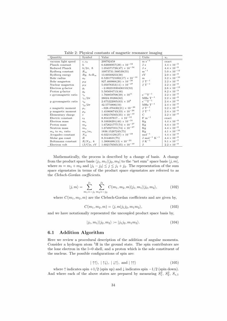
Table 2: Physical constants of magnetic resonance imagingQuantity Symbol Value Units ur
vacuum light speed c, c0 299792458 m s−1 exact
Planck constant h 6.62606957(29)× 10−34 J s 4.4× 10⁻⁸
Reduced Planck h/2π, ~ 1.054571726(47)× 10−34 J s 4.4× 10⁻⁸
Rydberg constant R∞ 10973731.568539(55) m−1 5.0× 10⁻¹²
Rydberg energy Ry, hcR∞ 13.60569253(30) eV 2.0× 10⁻⁸
Bohr radius a0 0.52917721092(17)× 10−10 m 3.2× 10⁻¹⁰
Bohr magneton µB 927.400968(20)× 10−26 J T−1 2.2× 10⁻⁸
Nuclear magneton µN 5.05078353(11)× 10−27 J T−1 2.2× 10⁻⁸
Electron g-factor ge −2.00231930436153(53) 2.6× 10⁻¹³
Proton g-factor gp 5.585694713(46) 8.2× 10⁻⁹
e gyromagnetic ratio γe 1.760859708(39)× 1011 s−1T−1 2.2× 10⁻⁸
γe/2π 28024.95266(62) MHz T−1 2.2× 10⁻⁸
p gyromagnetic ratio γp 2.675222005(63)× 108 s−1T−1 2.4× 10⁻⁸
γp/2π 42.5774806(10) MHz T−1 2.4× 10⁻⁸
e magnetic moment µe −928.476430(21)× 10−26 J T−1 2.2× 10⁻⁸
p magnetic moment µp 1.410606743(33)× 10−26 J T−1 2.4× 10⁻⁸
Elementary charge e 1.602176565(35)× 10−19 C 2.2× 10⁻⁸
Electric constant ε0 8.854187817...× 10−12 F m−1 exact
Electron mass me 9.10938291(40)× 10−31 Kg 4.4× 10⁻⁸
Proton mass mp 1.672621777(74)× 10−27 Kg 4.4× 10⁻⁸
Neutron mass mn 1.674927351(74)× 10−27 Kg 4.4× 10⁻⁸
mp to me ratio mp/me 1836.15267245(75) Kg 4.1× 10⁻¹⁰
Avogadro constant NA 6.02214129(27)× 10−23 mol−1 4.4× 10⁻⁸
Molar gas const R 8.3144621(75) J mol−1 K−1 4.4× 10⁻⁸
Boltzmann constant R/NA, k 1.3806488(13)× 10−23 J K−1 9.1× 10⁻⁷
Electron volt (J/C)e, eV 1.602176565(35)× 10−19 J 2.2× 10⁻⁸
Mathematically, the process is described by a change of basis. A changefrom the product space basis 〈j1,m1|〈j2,m2| to the “net sum” space basis 〈j,m|,where m = m1 +m2 and |j1 − j2| ≤ j ≤ j1 + j2. The representation of the sumspace eigenstates in terms of the product space eigenstates are referred to asthe Clebsch-Gordan coefficients.
|j,m〉 =
j1∑m1=−j1
j2∑m2=−j2
C(m1,m2,m)|j1,m1〉|j2,m2〉, (102)
where C(m1,m2,m) are the Clebsch-Gordan coefficients and are given by,
C(m1,m2,m) = 〈j,m|j1j2,m1m2〉, (103)
and we have notationally represented the uncoupled product space basis by,
|j1,m1〉|j2,m2〉 := |j1j2,m1m2〉. (104)
6.1 Addition Algorithm
Here we review a procedural description of the addition of angular momenta.Consider a hydrogen atom 1H in the ground state. The spin contributors arethe lone electron in the l=0 shell, and a proton which is the sole constituent ofthe nucleus. The possible configurations of spin are:
| ↑↑〉, | ↑↓〉, | ↓↑〉, and | ↑↑〉 (105)
where ↑ indicates spin +1/2 (spin up) and ↓ indicates spin −1/2 (spin down).And where each of the above states are prepared by measuring S2
1 , S22 , Sz,1
34

Table 3: Spherical Harmonics for l = 0, 1, 2, and 3.
l ml Ymll
0 0 Y 00 (θ, φ) = 1
2
√1π
1 -1 Y −11 (θ, φ) = 1
2
√32π
sin θe−iφ
1 0 Y 01 (θ, φ) = 1
2
√3π
cos θ
1 1 Y 11 (θ, φ) = − 1
2
√32π
sin θeiφ
2 -2 Y −22 (θ, φ) = 1
4
√152π
sin2 θe−2iφ
2 -1 Y −12 (θ, φ) = 1
2
√152π
sin θ cos θe−iφ
2 0 Y 02 (θ, φ) = 1
4
√5π
(3 cos2 θ − 1)
2 1 Y 12 (θ, φ) = − 1
2
√152π
sin θ cos θeiφ
2 2 Y 22 (θ, φ) = 1
4
√152π
sin2 θe2iφ
3 -3 Y −33 (θ, φ) = 1
8
√35π
sin3 θe−3iφ
3 -2 Y −23 (θ, φ) = 1
4
√1052π
sin2 θ cos θe−2iφ
3 -1 Y −13 (θ, φ) = 1
8
√21π
(5 cos2 θ − 1) sin θe−iφ
3 0 Y 03 (θ, φ) = 1
4
√7π
(5 cos3 θ − 3 cos θ)
3 1 Y 13 (θ, φ) = − 1
8
√21π
(5 cos2 θ − 1) sin θeiφ
3 2 Y 23 (θ, φ) = 1
4
√1052π
sin2 θ cos θe2iφ
3 3 Y 33 (θ, φ) = − 1
8
√35π
sin3 θe3iφ
and Sz,2 for each state. We are interested in the combined state of the twoparticle system, and this requires the quantum mechanical addition of angularmomenta, or in this example, spin. The net result is a state |s,m〉 whose spincan be determined by measuring S2 and whose z-component of spin can bedetermined by measuring Sz, where S = S1 + S2 and Sz = Sz,1 + Sz,2. Itfollows that m = m1 +m2, and therefore the possible values of m are 1, 0, 0, -1.This suggests a triplet state (s=1) and a singlet state (s=0). The triplet statecorresponds to m=1,0,-1, and is given by,
|1, 1〉 7→ | ↑↑〉|1, 0〉 7→ 1√
2(| ↑↓〉+ | ↓↑〉)
|1,−1〉 7→ | ↓↓〉(106)
and the singlet state corresponds to,
|0, 0〉 7→ 1√2
(| ↑↓〉 − | ↓↑〉), (107)
where upon designation of the top assignment |1, 1〉, each of the other statesare obtained by application of the ladder operators defined in Equation (99).For example,
S−|1, 1〉 = ~√
2|1, 0〉 (108)
To change to a representation in the uncoupled basis, we write,
35

Table 4: Radial Wave Functions for n = 0, 1, 2, and 3.
n l Rln
1 0 R01(r) = 2
(1a0
)3/2e−r/a0
2 0 R02(r) =
(1
2a0
)3/2(2 − r/a0)e−r/2a0
2 1 R12(r) =
(1
2a0
)3/2r
a0√3e−r/2a0
3 0 R03(r) = 2
(1
3a0
)3/2 (1 − 2r
3a0+ 2
27(r/a0)2
)e−r/3a0
3 1 R13(r) =
(1
3a0
)3/24√2
3
(1 − r
6a0
)e−r/3a0
3 2 R23(r) =
(1
3a0
)3/22√2
27√5
(ra0
)2e−r/3a0
|1, 0〉 =1
~√
2S−|1, 1〉 =
1
~√
2(S1,− + S2,−)| ↑↑〉, (109)
and therefore,
|1, 0〉 =1
~√
2(S1,−| ↑↑〉+ S2,−| ↑↑〉), (110)
which yields,
|1, 0〉 =1
~√
2(| ↓↑〉+ | ↑↓〉), (111)
Finally to obtain the singlet state, we simply orthogonalize the above, yield-ing,
|0, 0〉 =1
~√
2(| ↓↑〉 − | ↑↓〉) (112)
The above procedure is easily carried out by a computer for any combinationof particle spins. For many particle systems, for instance in the computation ofnuclear spins or non-ground state 1H configurations, the associativity propertyis used and the above description applies. In the above example, the factors 1
~√
2
are the Clebsch-Gordan coefficients. There are several openly available imple-mentations of Clebsch-Gordan coefficient calculators, in addition to tabulationsin handbooks of physics formulae [114, 1].
7 Group Theory: SO(3), SU(2), and SU(3)
Orbital angular momentum and spin are the source of magnetic resonance. Theirabstract mathematical description is group theoretic, and extends naturally intoother fundamental physics such as the strong interaction of quarks in nucle-ons and nucleons in nuclei. The Frenchman Henri Poincare commented that“mathematicians do not study objects, but the relationships between objects”.Relationships between symmetry groups have indeed been the essential devicefor probing the unseen in the realm of high energy particle physics.
For spin 1/2 particles such as the electron and the quark, the spin observablecan be represented by the SU(2) group. SU(N) is the group of N ×N unitary
36

matrices with unit determinant, in which the group operation is matrix-matrixmultiplication. Similarly SO(N) is the group of N ×N orthogonal matrices ofunit determinant, with matrix multiplication as group operator. Analogous tothe SU(2) representation of spin, quantum orbital angular momentum can berepresented by the SO(3) group. Both groups share a Lie Algebra, encoded inthe commutation relations shown above, because they are isomorphic to eachother. In particular, SU(2) is a double cover of SO(3). The SU(3) group modelsthe interactors of the strong force in Quantum Chromodynamics (QCD).
7.1 SO(3)
A counterclockwise rotation by an angle φ about the x, y, or z-axes, can respec-tively be represented by
Rx(φ) =
1 0 00 cosφ − sinφ0 sinφ cosφ
,
Ry(φ) =
cosφ 0 sinφ0 1 0
− sinφ 0 cosφ
,
Rz(φ) =
cosφ − sinφ 0sinφ cosφ 0
0 0 1
.
(113)
The corresponding infinitesimal generators, Gx, Gy, Gz respectively are:
0 0 00 0 −10 1 0
,
0 0 10 0 0−1 0 0
,
0 −1 01 0 00 0 0
. (114)
The corresponding Lie Algebra can then be readily shown to be:
[Gi, Gj ] = i~εijkGk (115)
7.2 SU(2)
SU(2) =
(a −b∗b a∗
): a, b ∈ C, a2 + b2 = 1
(116)
It follows that the generators of SU(2) are the Pauli Matrices given by,
σ1 =
(0 11 0
), σ2 =
(0 −ii 0
), σ3 =
(1 00 −1
), (117)
The SU(2) Lie Algebra is then prescribed by the following commutation andanti-commutation relations,
[σa, σb] = 2iεabcσc, (118)
37

and
σa, σb = 2δab · I + iεabcσc, (119)
which combine to give:
σaσb = δab · I + iεabcσc, (120)
where δab is the Kronecker delta and x, y := xy+yx is the anti-commutator.
7.2.1 SU(2) is Isomorphic to the 3-Sphere
Given U ∈ SU(2), such that,
U =
(a −b∗b a∗
),
We define an assignment, ζ, such that
ζ :
a 7→ x0 + ix3
b 7→ −x2 + ix1
, (121)
where x0, x1, x2, x3 ∈ <. It follows that,
U = x0I + ixpσp, (122)
where I is the 2× 2 identity matrix, σp are the Pauli matrices, and we haveused the Einstein summation notation over p.
det(U) = 1⇒ a2 + b2 = 1⇒ x20 + xpxp = 1⇒ x ∈ S3 (123)
ζ is a bijective homomorphism between SU(2) and S3. And this showsSU(2) is isomorphic to S3.
7.3 SU(3)
The generators of the SU(3) group are given by the Gell-Mann matrices:
λ1 =
0 1 01 0 00 0 0
, λ2 =
0 −i 0i 0 00 0 0
,
λ3 =
1 0 00 −1 00 0 0
, λ4 =
0 0 10 0 01 0 0
,
λ5 =
0 0 −i0 0 0i 0 0
, λ6 =
0 0 00 0 10 1 0
,
λ7 =
0 0 00 0 −i0 i 0
, λ8 = 1√3
1 0 00 1 00 0 −2
,
(124)
38

Then defining Tj =λj
2 , the commutation relations are,
[Ta, Tb] = i
8∑c=1
fabcTc, (125)
and
Ta, Tb =4
3δab + 2
8∑c=1
dabcTc, (126)
where fabc and dabc are the antisymmetric and symmetric structure constantsof SU(3) respectively.
8 Summary
Magnetic resonance imaging is an application of quantum mechanics which hasrevolutionized the practice of medicine. Electrons, protons, and neutrons aremagnets by virtue of their spin and orbital angular momentum. Tissue is madeof ensembles of such subatomic particles, and can be imaged by sensing theirresponses to applied magnetic fields. As discussed in this paper, a wide array ofMRI modalities exist, each of which derives contrast by specific perturbationsof the magnetization vector. The potential of MRI in the diagnosis and eventhe treatment of various diseases is far from fully realized. A quantum level un-derstanding of magnetic resonance technology is essential for further innovationin this field.
39

Acknowledgement
The author thanks his friends Henok T. Mebrahtu and Peter Q. Blair for read-ing this manuscript and providing helpful feedback. And he thanks them formany enjoyable physics conversations over coffee. He thanks Daniel Ennis formaking available his MATLAB code for plotting spherical harmonics. He thankshis lovely wife Lisa M. Odaibo for a helpful conversation on the clinical use ofmagnetic resonance spectroscopy in hypoxic-ischemic injury assessment in theneonate. And he especially thanks her for her love and support. The authorthanks his entire family, and celebrates his father, Dr. Stephen K. Odaibo, onhis birthday today. He thanks him for being a kind wonderful father and ex-ample. He thanks those who contributed and are contributing to his education,including: Dr. Robert A. Copeland Jr., Dr. Leslie Jones, Dr. Janine Smith-Marshall, Dr. Bilal Khan, Dr. David Katz, Dr. Earl Kidwell, Dr. WilliamDeegan, Dr. Brian Brooks, Dr. Natalie Afshari, Dr. Isaac O. Karikari, Dr.Xiaobai Sun, Dr. Mark Dewhirst, Dr. Carlo Tomasi, Dr. John Kirkpatrick, Dr.Nicole Larrier, Dr. Brenda Armstrong, Dr. Phil Goodman, Dr. Joanne Wilsonand Dr. Ken Wilson, Dr. Srinivasan Mukunduan Jr., Dr. David Simel, Dr.Danny O. Jacobs, Dr. Timothy Elston, Drs. Akwari, Drs. Haynes, Dr. JohnMayer, Dr. Lex Oversteegen, Dr. Peter V. O’Neil, Dr. Anne Cusic, Dr. Henryvan den Bedem, Dr. James R. Ward, Dr. Marius Nkashama, Dr. Michael W.Quick, Dr. Robert J. Lefkowitz, Dr. Arlie Petters, and several other excellenteducators and role models not mentioned here.
40

Appendix A
Signals processing plays an important role in magnetic resonance imaging, andis briefly reviewed in this appendix. The free inductance decay signal is oftencollected in the frequency domain and Fourier transformed into the time do-main [35]. Also with a gradual shift towards MRI scanners of higher magneticfield, the signal-to-noise ratio requires increasingly more effective noise filter-ing algorithms. As signal generation and collection methods become increas-ingly more sophisticated e.g via spirals and other geometric sequences, non-uniform sampling, and exotic B1 pulse sequence configurations, signals process-ing methods need to advance in tandem to address problems arising. Computingspeed also takes on new significance with such developments. Indeed imagingand graphics applications have significantly driven the interest and funding forfast algorithms and computing. Notable advancements include the fast Fouriertransform, the fast-multipole method of Greengard and Rokhlin [40, 41], andparallel computing hardware such as the Compute Unified Device Architecture(CUDA) multi-core processors by Nvidia for graphics processing [86]. Further-more, a new field is taking form at the interface of high performance softwarealgorithms and multi-core hardware processors [83, 65, 82, 45, 87, 51].
We take a brief look at some of the basics of signals processing below,
A.1 Continuous and Discrete Fourier Transforms
The Fourier transform converts a time domain signal to its corresponding fre-quency domain signal, and is given by,
F [f(t)] = f(ω) =
∫ ∞−∞
f(t)e−iωtdt, (127)
while the inverse Fourier transform converts a frequency domain signal toits corresponding time domain signal, and is given by,
F−1[f(ω)] = f(t) =
∫ ∞−∞
f(ω)eiωtdω. (128)
In practice, the discrete versions of the above equations are used instead,and give good results provided that signal data is sampled at an appropriatefrequency, the Nyquist frequency. Given an MRI signal of N sample points,f [n], where n = 0, .., N −1, the frequency domain representation is given by thediscrete Fourier transform,
f [ωk] =
N−1∑n=0
f [n]e−i2πkN n, (129)
and the discrete inverse Fourier transform is given by,
f [n] =1
N
N−1∑k=0
f [ωk]ei2πkN n. (130)
The above Fourier formulas readily allow extension to two and three dimen-sions as well as various other customizations, tailored to suite the particularMRI application and data format.
41

A.2 MRI Sampling and the Aliasing Problem
Figure 24: 3D sinc function
The Whittaker- Kotelnikov- Shannon- Raabe- Someya- Nyquist theorem pre-scribes a lower bound on the sampling frequency necessary for perfect recon-struction of a band-limited signal. It states that given a band limited signalg(t) whose frequency domain representation is such that |g(f)| < B for all fand some B, then by sampling at a rate fs = 2B, the image can be perfectlyreconstructed. The sampling interval is T = 1/fs, and the discrete time signalis expressed as g[nT ] where n is an integer. fs = ωs/2π and is in units of hertz,hence T is in seconds. The perfect reconstruction is given by the Whittaker-Shannon interpolation formula,
g(t) =
∞∑n=−∞
g[nT ] · sinc
(t− nTT
), (131)
where sinc is the normalized sampling function given by,
sinc(x) =
1 if x = 0,sin(πx)
πxotherwise.
(132)
In practice, low-pass filtering methods can be used to decrease the amplitudeof frequency components which exceed the effective bandlimit.
The aliasing problem arises when the sampling rate fs is less than twice thebandlimit B. The effect of this is that the reconstructed image is an alias ofthe actual image. The Discrete Time Fourier Transform (DTFT) of a signal isgiven by,
42

X(ω) =
∞∑n=−∞
x[n]e−iωn, (133)
and in the case of an under-sampled MRI signal, the DTFT matches thatof the alias. Therefore the reconstructed image is merely an alias. This phe-nomenon can be described more formally by invoking the poisson summationformula,
Xs(f) :=
∞∑−∞
X(f − kfs) =
∞∑−∞
T · x(nT )e−i2πfnT , (134)
where the middle term above is the periodic summation. For a bandlim-ited under-sampled signal, increasing the sampling rate to satisfy the Nyquistcriterion will restore perfect reconstruction.
A.3 The Convolution Theorem
The convolution theorem facilitates application-specific image processing beforeor after reconstruction in either k-space or time domain. The theorem is givenby,
F(f ∗ g)(t) = f(ω) · g(ω), (135)
and states that the Fourier transform of the convolution of two functionsequals the product of the Fourier transforms of both functions. Where theconvolution is defined as,
(f ∗ g)(t) :=
∫ ∞−∞
f(τ)g(t− τ)dτ. (136)
43

References
[1] M. Abramowitz and I. A. Stegun, Handbook of mathematical functions:with formulas, graphs, and mathematical tables, vol. 55, Courier DoverPublications, 1964.
[2] H. Ay, F. S. Buonanno, G. Rordorf, P. W. Schaefer, L. H. Schwamm,O. Wu, R. G. Gonzalez, K. Yamada, G. A. Sorensen, and W. J. Koroshetz,Normal diffusion-weighted MRI during stroke-like deficits, Neurology 52(1999), no. 9, 1784–1784.
[3] D. Azzopardi, J. S. Wyatt, E. B. Cady, D. T. Delpy, J. Baudin, A. L.Stewart, P. L. Hope, P. A. Hamilton, and E. O. R. Reynolds, Prognosis ofnewborn infants with hypoxic-ischemic brain injury assessed by phosphorusmagnetic resonance spectroscopy, Pediatric Research 25 (1989), no. 5,445–451.
[4] M. Babic, D. Horak, P. Jendelova, V. Herynek, V. Proks, V. Vanecek,P. Lesny, and E. Sykova, The use of dopamine-hyaluronate associate-coated maghemite nanoparticles to label cells, International Journal ofNanomedicine 7 (2012), 1461.
[5] P. A. Bandettini and E. C. Wong, A hypercapnia-based normalizationmethod for improved spatial localization of human brain activation withfMRI, NMR in Biomedicine 10 (1997), no. 4-5, 197–203.
[6] P. A. Barber, D. G. Darby, P. M. Desmond, Q. Yang, R. P. Gerraty, D. Jol-ley, G. A. Donnan, B. M. Tress, and S. M. Davis, Prediction of stroke out-come with echoplanar perfusion-and diffusion-weighted MRI, Neurology51 (1998), no. 2, 418–426.
[7] J. Bardeen, Theory of the meissner effect in superconductors, PhysicalReview 97 (1955), no. 6, 1724.
[8] J. Bardeen, L. N. Cooper, and J. R. Schrieffer, Microscopic theory ofsuperconductivity, Physical Review 106 (1957), no. 1, 162–164.
[9] , Theory of superconductivity, Physical Review 108 (1957), no. 5,1175.
[10] A. J. Barkovich, K. D. Westmark, H. S. Bedi, J. C. Partridge, D. M. Fer-riero, and D. B. Vigneron, Proton spectroscopy and diffusion imaging onthe first day of life after perinatal asphyxia: preliminary report, AmericanJournal of Neuroradiology 22 (2001), no. 9, 1786–1794.
[11] P. Barzo, A. Marmarou, P. Fatouros, K. Hayasaki, and F. Corwin, Con-tribution of vasogenic and cellular edema to traumatic brain swelling mea-sured by diffusion-weighted imaging, Journal of Neurosurgery 87 (1997),no. 6, 900–907.
[12] C. L. Bennett, Z. P. Qureshi, A. O. Sartor, L. A. B. Norris, A. Murday,S. Xirasagar, and H.S . Thomsen, Gadolinium-induced nephrogenic sys-temic fibrosis: the rise and fall of an iatrogenic disease, Clinical KidneyJournal 5 (2012), no. 1, 82–88.
44

[13] M. A. Bernstein, K. F. King, and X. J. Zhou, Handbook of MRI pulsesequences, Academic Press, 2004.
[14] M. N. Biltcliffe, P. E. Hanley, J. B. McKinnon, and P. Roubeau, The oper-ation of superconducting magnets at temperatures below 4.2 k, Cryogenics12 (1972), no. 1, 44–47.
[15] F. Binkofski and R. J. Seitz, Modulation of the BOLD-response in earlyrecovery from sensorimotor stroke, Neurology 63 (2004), no. 7, 1223–1229.
[16] E. Brucher, Kinetic stabilities of gadolinium (III) chelates used as MRIcontrast agents, Contrast Agents I (2002), 103–122.
[17] J. W. M. Bulte and D. L. Kraitchman, Iron oxide MR contrast agents formolecular and cellular imaging, NMR in Biomedicine 17 (2004), no. 7,484–499.
[18] K. Butcher, M. Parsons, T. Baird, A. Barber, G. Donnan, P. Desmond,B. Tress, and S. Davis, Perfusion thresholds in acute stroke thrombolysis,Stroke 34 (2003), no. 9, 2159–2164.
[19] C. Calautti and J. C. Baron, Functional neuroimaging studies of motorrecovery after stroke in adults, Stroke 34 (2003), no. 6, 1553–1566.
[20] M. Cappellini, G. Rapisardi, M. L. Cioni, and C. Fonda, Acute hypoxic en-cephalopathy in the full-term newborn: correlation between magnetic res-onance spectroscopy and neurological evaluation at short and long term.,La Radiologia medica 104 (2002), no. 4, 332.
[21] P. Caravan, Strategies for increasing the sensitivity of gadolinium basedMRI contrast agents, Chem. Soc. Rev. 35 (2006), no. 6, 512–523.
[22] , Protein-targeted gadolinium-based magnetic resonance imaging(MRI) contrast agents: design and mechanism of action, Accounts ofchemical research 42 (2009), no. 7, 851–862.
[23] P. Caravan, J. J. Ellison, T. J. McMurry, and R. B. Lauffer, Gadolinium(III) chelates as MRI contrast agents: structure, dynamics, and applica-tions, Chemical Reviews 99 (1999), no. 9, 2293–2352.
[24] S. C. Chang, P. H. Lai, W. L. Chen, H. H. Weng, J. T. Ho, J. S. Wang,C. Y. Chang, H. B. Pan, and C. F. Yang, Diffusion-weighted MRI featuresof brain abscess and cystic or necrotic brain tumors: comparison withconventional MRI, Clinical imaging 26 (2002), no. 4, 227–236.
[25] L. N. Cooper, Bound electron pairs in a degenerate Fermi gas, PhysicalReview 104 (1956), no. 4, 1189.
[26] S. B. Coutts, J. E. Simon, A. I. Tomanek, P. A. Barber, J. Chan, M. E.Hudon, J. R. Mitchell, R. Frayne, M. Eliasziw, A. M. Buchan, and A. M.Demchuk, Reliability of assessing percentage of diffusion-perfusion mis-match, Stroke 34 (2003), no. 7, 1681–1683.
45

[27] S. C. Cramer, R. Shah, J. Juranek, K. R. Crafton, and V. Le, Activity inthe peri-infarct rim in relation to recovery from stroke, Stroke 37 (2006),no. 1, 111–115.
[28] R. A. Crisostomo, M. M. Garcia, and D. C. Tong, Detection of diffusion-weighted MRI abnormalities in patients with transient ischemic attack,Stroke 34 (2003), no. 4, 932–937.
[29] E. J. Cukauskas, D. A. Vincent, and B. S. Deaver, Magnetic susceptibilitymeasurements using a superconducting magnetometer, Review of ScientificInstruments 45 (1974), no. 1, 1–6.
[30] R. Damadian, Tumor detection by nuclear magnetic resonance, Science171 (1971), no. 3976, 1151–1153.
[31] R. Damadian, K. Zaner, D. Hor, T. DiMaio, L. Minkoff, and M. Gold-smith, Nuclear magnetic resonance as a new tool in cancer research: hu-man tumors by nmr, Annals of the New York Academy of Sciences 222(1973), no. 1, 1048–1076.
[32] R. V. Damadian, Apparatus and method for detecting cancer in tissue,1974, US Patent 3,789,832.
[33] C. L. Dumoulin and H. R. Hart Jr, Magnetic resonance angiography.,Radiology 161 (1986), no. 3, 717–720.
[34] C. L. Dumoulin, S. P. Souza, M. F. Walker, and W. Wagle, Three-dimensional phase contrast angiography, Magnetic Resonance in Medicine9 (1989), no. 1, 139–149.
[35] R. R. Ernst and W. A. Anderson, Application of fourier transform spec-troscopy to magnetic resonance, Review of Scientific Instruments 37(1966), no. 1, 93–102.
[36] J. Faiz Kayyem, R. M. Kumar, S. E. Fraser, and T. J. Meade, Receptor-targeted co-transport of DNA and magnetic resonance contrast agents,Chemistry & biology 2 (1995), no. 9, 615–620.
[37] D. N. Firmin, G. L. Nayler, P. J. Kilner, and D. B. Longmore, The appli-cation of phase shifts in NMR for flow measurement, Magnetic Resonancein Medicine 14 (1990), no. 2, 230–241.
[38] B. S. Geisler, F. Brandhoff, J. Fiehler, C. Saager, O. Speck, J. Rother,H. Zeumer, and T. Kucinski, Blood oxygen level–dependent MRI allowsmetabolic description of tissue at risk in acute stroke patients, Stroke 37(2006), no. 7, 1778–1784.
[39] C. B. Grandin, T. P. Duprez, A. M. Smith, C. Oppenheim, A. Peeters,A. R. Robert, and G. Cosnard, Which MR-derived perfusion parametersare the best predictors of infarct growth in hyperacute stroke? compara-tive study between relative and quantitative measurements, Radiology 223(2002), no. 2, 361–370.
[40] L. Greengard and V. Rokhlin, A fast algorithm for particle simulations,Journal of Computational Physics 73 (1987), no. 2, 325–348.
46
[41] , A new version of the fast multipole method for the laplace equationin three dimensions, Acta Numerica 6 (1997), no. 1, 229–269.
[42] O. H. J. Grohn and R. A. Kauppinen, Assessment of brain tissue viabilityin acute ischemic stroke by BOLD MRI, NMR in Biomedicine 14 (2001),no. 7-8, 432–440.
[43] F. Hamzei, R. Knab, C. Weiller, and J. Rother, The influence of extra-andintracranial artery disease on the BOLD signal in FMRI, Neuroimage 20(2003), no. 2, 1393–1399.
[44] P. Hanover and B. Eilhardt, Conductor system for superconducting cables,January 1 1972, US Patent 3,634,597.
[45] P. Harish and P. Narayanan, Accelerating large graph algorithms on theGPU using CUDA, High Performance Computing–HiPC 2007 (2007),197–208.
[46] M. Hermier and N. Nighoghossian, Contribution of susceptibility-weightedimaging to acute stroke assessment, Stroke 35 (2004), no. 8, 1989–1994.
[47] M. L. Hugh, Low temperature electric transmission systems, 1971, USPatent 3,562,401.
[48] G. E. Jackson, S. Wynchank, and M. Woudenberg, Gadolinium (III) com-plex equilibria: the implications for Gd (III) MRI contrast agents, Mag-netic resonance in medicine 16 (1990), no. 1, 57–66.
[49] C. W. Jung and P. Jacobs, Physical and chemical properties of super-paramagnetic iron oxide MR contrast agents: ferumoxides, ferumoxtran,ferumoxsil, Magnetic resonance imaging 13 (1995), no. 5, 661–674.
[50] G. W. Kabalka, E. Buonocore, K. Hubner, M. Davis, andL. Huang, Gadolinium-labeled liposomes containing paramagnetic amphi-pathic agents: Targeted MRI contrast agents for the liver, Magnetic reso-nance in medicine 8 (1988), no. 1, 89–95.
[51] S. Kestur, K. Irick, S. Park, A. Al Maashri, V. Narayanan, andC. Chakrabarti, An algorithm-architecture co-design framework for grid-ding reconstruction using FPGAs, Design Automation Conference (DAC),2011 48th ACM/EDAC/IEEE, IEEE, 2011, pp. 585–590.
[52] Y. R. Kim, I. J. Huang, S. R. Lee, E. Tejima, J. B. Mandeville, M. P. A.van Meer, G. Dai, Y. W. Choi, R. M. Dijkhuizen, E. H. Lo, and B. R.Rosen, Measurements of BOLD/CBV ratio show altered fMRI hemody-namics during stroke recovery in rats, Journal of Cerebral Blood Flow &Metabolism 25 (2005), no. 7, 820–829.
[53] H. Kobayashi, M. W. Brechbiel, et al., Dendrimer-based macromolecularMRI contrast agents: characteristics and application., Molecular imaging2 (2003), no. 1, 1.
47

[54] S. D. Konda, M. Aref, S. Wang, M. Brechbiel, and E. C. Wiener, Specifictargeting of folate–dendrimer MRI contrast agents to the high affinity fo-late receptor expressed in ovarian tumor xenografts, Magnetic ResonanceMaterials in Physics, Biology and Medicine 12 (2001), no. 2, 104–113.
[55] P. H. Kuo, E. Kanal, A. K. Abu-Alfa, and S. E. Cowper, Gadolinium-based MR contrast agents and nephrogenic systemic fibrosis, Radiology242 (2007), no. 3, 647–649.
[56] S. M. Lai, T. Y. Tsai, C. Y. Hsu, J. L. Tsai, M. Y. Liao, and P. S.Lai, Bifunctional silica-coated superparamagnetic FePt nanoparticles forfluorescence/MR dual imaging, Journal of Nanomaterials 2012 (2012), 5.
[57] J. A. Langlois, W. Rutland-Brown, and M. M. Wald, The epidemiologyand impact of traumatic brain injury: a brief overview, The Journal ofHead Trauma Rehabilitation 21 (2006), no. 5, 375–378.
[58] P. C. Lauterbur et al., Image formation by induced local interactions:examples employing nuclear magnetic resonance, Nature 242 (1973),no. 5394, 190–191.
[59] N. Lee, Y. Choi, Y. Lee, M. Park, W. K. Moon, S. H. Choi, and T. Hyeon,Water-dispersible ferrimagnetic iron oxide nanocubes with extremely highr 2 relaxivity for highly sensitive in vivo MRI of tumors, Nano letters 12(2012), no. 6, 3127–3131.
[60] D. R. Lide, CRC handbook of chemistry and physics, CRC press, 2012.
[61] M. J. Lipinski, V. Amirbekian, J. C. Frias, J. G. S. Aguinaldo, V. Mani,K. C. Briley-Saebo, V. Fuster, J. T. Fallon, E. A. Fisher, and Z. A.Fayad, MRI to detect atherosclerosis with gadolinium-containing immu-nomicelles targeting the macrophage scavenger receptor, Magnetic reso-nance in medicine 56 (2006), no. 3, 601–610.
[62] A. Y. Liu, J. A. Maldjian, L. J. Bagley, G. P. Sinson, and R. I. Grossman,Traumatic brain injury: diffusion-weighted MR imaging findings, Ameri-can Journal of Neuroradiology 20 (1999), no. 9, 1636–1641.
[63] D. H. Live and S. I. Chan, Bulk susceptibility corrections in nuclear mag-netic resonance experiments using superconducting solenoids, AnalyticalChemistry 42 (1970), no. 7, 791–792.
[64] G. K. Malik, M. Pandey, R. Kumar, S. Chawla, B. Rathi, and R. K. Gupta,MR imaging and in vivo proton spectroscopy of the brain in neonateswith hypoxic ischemic encephalopathy, European Journal of Radiology 43(2002), no. 1, 6–13.
[65] S.A. Manavski, CUDA compatible GPU as an efficient hardware accelera-tor for AES cryptography, Signal Processing and Communications, 2007.ICSPC 2007. IEEE International Conference on, IEEE, 2007, pp. 65–68.
[66] D. M. Mandell, J. S. Han, J. Poublanc, A. P. Crawley, J. A. Stainsby,J. A. Fisher, and D. J. Mikulis, Mapping cerebrovascular reactivity usingblood oxygen level-dependent MRI in patients with arterial steno-occlusivedisease, Stroke 39 (2008), no. 7, 2021–2028.
48

[67] C. Maneru, C. Junque, N. Bargallo, M. Olondo, F. Botet, M. Tallada,J. Guardia, and J. M. Mercader, 1H-MR spectroscopy is sensitive to subtleeffects of perinatal asphyxia, Neurology 57 (2001), no. 6, 1115–1118.
[68] P. Marckmann, L. Skov, K. Rossen, A. Dupont, M. B. Damholt, J. G.Heaf, and H. S. Thomsen, Nephrogenic systemic fibrosis: suspectedcausative role of gadodiamide used for contrast-enhanced magnetic reso-nance imaging, Journal of the American Society of Nephrology 17 (2006),no. 9, 2359–2362.
[69] M. P. Marks, D. C. Tong, C. Beaulieu, G. W. Albers, A. De Crespigny,and M. E. Moseley, Evaluation of early reperfusion and IV tPA therapyusing diffusion-and perfusion-weighted MRI, Neurology 52 (1999), no. 9,1792–1792.
[70] H. T. Mebrahtu, I. V. Borzenets, D. E. Liu, H. Zheng, Y. V. Bomze, A. I.Smirnov, H. U. Baranger, and G. Finkelstein, Quantum phase transition ina resonant level coupled to interacting leads, Nature 488 (2012), no. 7409,61–64.
[71] R. W. Meyerhoff, Superconducting power transmission, Cryogenics 11(1971), no. 2, 91–101.
[72] M. Mikawa, H. Kato, M. Okumura, M. Narazaki, Y. Kanazawa, N. Miwa,and H. Shinohara, Paramagnetic water-soluble metallofullerenes havingthe highest relaxivity for MRI contrast agents, Bioconjugate chemistry 12(2001), no. 4, 510–514.
[73] J. Mintorovitch, M. E. Moseley, L. Chileuitt, H. Shimizu, Y. Cohen, andP. R. Weinstein, Comparison of diffusion-and T2-weighted MRI for theearly detection of cerebral ischemia and reperfusion in rats, Magnetic res-onance in medicine 18 (1991), no. 1, 39–50.
[74] M. Miyazaki, S. Sugiura, F. Tateishi, H. Wada, Y. Kassai, and H. Abe,Non-contrast-enhanced MR angiography using 3D ECG-synchronized half-fourier fast spin echo, Journal of Magnetic Resonance Imaging 12 (2000),no. 5, 776–783.
[75] P. J. Mohr, B. N. Taylor, and D. B. Newell, Codata recommended val-ues of the fundamental physical constants: 2010. 2012, E-print: arXiv.org/abs/1203.5425.
[76] B. Morgan, A. L. Thomas, J. Drevs, J. Hennig, M. Buchert, A. Jivan,M. A. Horsfield, K. Mross, H. A. Ball, L. Lee, et al., Dynamic contrast-enhanced magnetic resonance imaging as a biomarker for the pharmaco-logical response of PTK787/ZK 222584, an inhibitor of the vascular en-dothelial growth factor receptor tyrosine kinases, in patients with advancedcolorectal cancer and liver metastases: results from two phase I studies,Journal of clinical oncology 21 (2003), no. 21, 3955–3964.
[77] M. E. Moseley, Y. Cohen, J. Mintorovitch, L. Chileuitt, H. Shimizu,J. Kucharczyk, M. F. Wendland, and P. R. Weinstein, Early detec-tion of regional cerebral ischemia in cats: comparison of diffusion-and
49

T2-weighted MRI and spectroscopy, Magnetic resonance in medicine 14(1990), no. 2, 330–346.
[78] Y. Murata, K. Sakatani, T. Hoshino, N. Fujiwara, T. Kano, S. Naka-mura, and Y. Katayama, Effects of cerebral ischemia on evoked cerebralblood oxygenation responses and BOLD contrast functional MRI in strokepatients, Stroke 37 (2006), no. 10, 2514–2520.
[79] C. J. L. Murray, A. D. Lopez, et al., Global mortality, disability, and thecontribution of risk factors: Global Burden of Disease Study, Lancet 349(1997), no. 9063, 1436–1442.
[80] T. Neumann-Haefelin, H. J. Wittsack, F. Wenserski, M. Siebler, R. J.Seitz, U. Modder, and H. J. Freund, Diffusion-and perfusion-weightedMRI: the DWI/PWI mismatch region in acute stroke, Stroke 30 (1999),no. 8, 1591–1597.
[81] E. A. Neuwelt, B. E. Hamilton, C. G. Varallyay, W. R. Rooney, R. D. Edel-man, P. M. Jacobs, and S. G. Watnick, Ultrasmall superparamagnetic ironoxides (USPIOs): a future alternative magnetic resonance (MR) contrastagent for patients at risk for nephrogenic systemic fibrosis (NSF) &quest,Kidney international 75 (2008), no. 5, 465–474.
[82] J. Nickolls, I. Buck, M. Garland, and K. Skadron, Scalable parallel pro-gramming with CUDA, Queue 6 (2008), no. 2, 40–53.
[83] A. Nukada, Y. Ogata, T. Endo, and S. Matsuoka, Bandwidth intensive3-D FFT kernel for GPUs using CUDA, High Performance Computing,Networking, Storage and Analysis, 2008. SC 2008. International Confer-ence for, IEEE, 2008, pp. 1–11.
[84] National Academies (US). Committee on Facilitating Interdisciplinary Re-search, Committee on Science, Engineering, Public Policy (US), Instituteof Medicine (US), and National Academy of Engineering, Facilitating in-terdisciplinary research, National Academy Press, 2005.
[85] N.D. Opdyke and V. Mejia, Earth’s magnetic field, Geophysical Mono-graph Series 145 (2004), 315–320.
[86] L. Pan, L. Gu, and J. Xu, Implementation of medical image segmentationin CUDA, Information Technology and Applications in Biomedicine, 2008.ITAB 2008. International Conference on, IEEE, 2008, pp. 82–85.
[87] G. Papamakarios, G. Rizos, N .P. Pitsianis, and X. Sun, Fast computationof local correlation coefficients on graphics processing units, Proc. of SPIEVol, vol. 7444, 2009, pp. 744412–1.
[88] M. W. Parsons, P. A. Barber, J. Chalk, D. G. Darby, S. Rose, P. M.Desmond, R. P. Gerraty, B. M. Tress, P. M. Wright, G. A. Donnan, andS. M. Davis, Diffusion-and perfusion-weighted MRI response to thrombol-ysis in stroke, Annals of Neurology 51 (2002), no. 1, 28–37.
[89] J. E. Perthen, F. Calamante, D. G. Gadian, and A. Connelly, Is quan-tification of bolus tracking MRI reliable without deconvolution?, Magneticresonance in medicine 47 (2002), no. 1, 61–67.
50
[90] O. A. C. Petroff, J. W. Prichard, K. L. Behar, J. R. Alger, J. A. denHollander, and R. G. Shulman, Cerebral intracellular pH by 31P nuclearmagnetic resonance spectroscopy, Neurology 35 (1985), no. 6, 781–781.
[91] J. M. Provenzale, R. D. Tien, G. J. Felsberg, and L. Hacein-Bey, Spinaldural arteriovenous fistula: demonstration using phase contrast MRA.,Journal of Computer Assisted Tomography 18 (1994), no. 5, 811.
[92] K. N. Raymond, V. C. Pierre, et al., Next generation, high relaxivitygadolinium MRI agents, Bioconjugate chemistry 16 (2005), no. 1, 3–8.
[93] G. Rordorf, W. J. Koroshetz, W. A. Copen, S. C. Cramer, P. W. Schaefer,R. F. Budzik, L. H. Schwamm, F. Buonanno, A. G. Sorensen, and G. Gon-zalez, Regional ischemia and ischemic injury in patients with acute middlecerebral artery stroke as defined by early diffusion-weighted and perfusion-weighted MRI, Stroke 29 (1998), no. 5, 939–943.
[94] H. J. Rosen, S. E. Petersen, M. R. Linenweber, A. Z. Snyder, D. A. White,L. Chapman, A. W. Dromerick, J. A. Fiez, and M. Corbetta, Neuralcorrelates of recovery from aphasia after damage to left inferior frontalcortex, Neurology 55 (2000), no. 12, 1883–1894.
[95] M. Rovaris, A. Gass, R. Bammer, S. J. Hickman, O. Ciccarelli, D. H.Miller, and M. Filippi, Diffusion MRI in multiple sclerosis, Neurology 65(2005), no. 10, 1526–1532.
[96] W. Rutland-Brown, J. A. Langlois, K. E. Thomas, and Y. L. Xi, Incidenceof traumatic brain injury in the United States, 2003, The Journal of HeadTrauma Rehabilitation 21 (2006), no. 6, 544.
[97] C. Rydahl, H. S. Thomsen, and P. Marckmann, High prevalence of nephro-genic systemic fibrosis in chronic renal failure patients exposed to gado-diamide, a gadolinium-containing magnetic resonance contrast agent, In-vestigative radiology 43 (2008), no. 2, 141.
[98] G. Schlaug, A. Benfield, A. E. Baird, B. Siewert, K. O. Lovblad, R. A.Parker, R. R. Edelman, and S. Warach, The ischemic penumbra, Neurol-ogy 53 (1999), no. 7, 1528–1528.
[99] L. C. Shih, J. L. Saver, J. R. Alger, S. Starkman, M. C. Leary, F. Vin-uela, G. Duckwiler, Y. P. Gobin, R. Jahan, J. P. Villablanca, P. M. Vespa,and C. S. Kidwell, Perfusion-weighted magnetic resonance imaging thresh-olds identifying core, irreversibly infarcted tissue, Stroke 34 (2003), no. 6,1425–1430.
[100] M. B. Singer, J. Chong, D. Lu, W. J. Schonewille, S. Tuhrim, and S. W.Atlas, Diffusion-weighted MRI in acute subcortical infarction, Stroke 29(1998), no. 1, 133–136.
[101] M. B. Stearns, Spin-echo and free-induction-decay measurements in pureFe and Fe-rich ferromagnetic alloys: Domain-wall dynamics, Physical Re-view 162 (1967), no. 2, 496.
51

[102] G. Strangman, J. P. Culver, J. H. Thompson, and D. A. Boas, A quantita-tive comparison of simultaneous BOLD fMRI and NIRS recordings duringfunctional brain activation, Neuroimage 17 (2002), no. 2, 719–731.
[103] A. Sturzu, S. Sheikh, U. Klose, M. Deeg, H. Echner, T. Nagele, U. Erne-mann, and S. Heckl, Novel gastrin receptor-directed contrast agents-potential in brain tumor magnetic resonance imaging, Medicinal Chem-istry 8 (2012), no. 2, 133–137.
[104] T. Sugahara, Y. Korogi, M. Kochi, I. Ikushima, Y. Shigematu, T. Hirai,T. Okuda, L. Liang, Y. Ge, Y. Komohara, et al., Usefulness of diffusion-weighted MRI with echo-planar technique in the evaluation of cellularityin gliomas, Journal of magnetic resonance imaging 9 (1999), no. 1, 53–60.
[105] V. N. Thijs, D. M. Somford, R. Bammer, W. Robberecht, M. E. Mose-ley, and G. W. Albers, Influence of arterial input function on hypoperfu-sion volumes measured with perfusion-weighted imaging, Stroke 35 (2004),no. 1, 94–98.
[106] H. S. Thomsen, Nephrogenic systemic fibrosis: a serious late adverse re-action to gadodiamide, European radiology 16 (2006), no. 12, 2619–2621.
[107] P. Thullen, J. C. Dudley, D. L. Greene, J. L. Smith, and H. H. Woodson,An experimental alternator with a superconducting rotating field winding,Power Apparatus and Systems, IEEE Transactions on (1971), no. 2, 611–619.
[108] D. C. Tong, M. A. Yenari, G. W. Albers, M. O’brien, M. P. Marks, andM. E. Moseley, Correlation of perfusion-and diffusion-weighted MRI withNIHSS score in acute (< 6.5 hour) ischemic stroke, Neurology 50 (1998),no. 4, 864–869.
[109] C. Tu and A. Y. Louie, Nanoformulations for molecular MRI, Wiley In-terdisciplinary Reviews: Nanomedicine and Nanobiotechnology (2012).
[110] F. H. R van der Zande, P. A. M Hofman, and W. H. Backes, Mappinghypercapnia-induced cerebrovascular reactivity using BOLD MRI, Neuro-radiology 47 (2005), no. 2, 114–120.
[111] Z. Wang, J. M. van Oort, and M. X. Zou, Development of superconductingmagnet for high-field MR systems in China, Physica C: Superconductivity(2012).
[112] E. C. Wiener, S. Konda, A. Shadron, M. Brechbiel, and O. Gansow, Tar-geting dendrimer-chelates to tumors and tumor cells expressing the high-affinity folate receptor, Investigative Radiology 32 (1997), no. 12, 748.
[113] W. Wiltschko and R. Wiltschko, Magnetic compass of european robins,Science 176 (1972), no. 4030, 62–64.
[114] G. Woan, The cambridge handbook of physics formulas, Cambridge UnivPr, 2000.
52

[115] O. Wu, W. J. Koroshetz, L. Ustergaard, F. S. Buonanno, W. A. Copen,R. G. Gonzalez, G. Rordorf, B. R. Rosen, L. H. Schwamm, R. M. Weis-skoff, and A. G. Sorensen, Predicting tissue outcome in acute human cere-bral ischemia using combined diffusion-and perfusion-weighted MR imag-ing, Stroke 32 (2001), no. 4, 933–942.
[116] K. Yamada, O. Wu, R. G. Gonzalez, D. Bakker, L. Østergaard, W. A.Copen, R. M. Weisskoff, B. R. Rosen, K. Yagi, T. Nishimura, and A. G.Sorensen, Magnetic resonance perfusion-weighted imaging of acute cere-bral infarction, Stroke 33 (2002), no. 1, 87–94.
[117] H. Zhu, D. G. Buck, Z. Zhang, H. Zhang, P. Wang, V. A. Stenger, M. R.Prince, and Y. Wang, High temporal and spatial resolution 4D MRA usingspiral data sampling and sliding window reconstruction, Magnetic Reso-nance in Medicine 52 (2004), no. 1, 14–18.
53

Author Biography
Dr. Stephen G. Odaibo is Chief Executive Officer and Founder of Quantum Lucid
Research Laboratories. He is a Mathematician, Computer scientist, Physicist, Bio-
chemist, and Physician. Dr. Odaibo obtained a B.S. in Mathematics (UAB, 2001),
M.S. in Mathematics (UAB, 2002), M.S. in Computer Science (Duke, 2009), and
Doctor of Medicine (Duke, 2010). He completed a two year pre-doctoral research
fellowship in Biochemistry in affiliation with the Howard Hughes Medical Institute
between 2004 and 2006, during which he studied cell signaling. Dr. Odaibo completed
a housemanship in Internal Medicine at Duke University Hospital and is currently an
Ophthalmology resident at Howard University Hospital in Washington DC. His awards
and recognitions include: he invented the Trajectron method and provided the first
quantitative demonstration of non-paraxial light bending within the human cornea;
his first paper was selected by MIT Technology Review as one of the best papers from
Physics or Computer science submitted to the arXiv the first week of Oct 2011; he
was an Invited Discussant to the exclusive launching of the U.S. National Academy
of Sciences Committee Report, Optics and Photonics: Essential Technologies for Our
Nation; he won the Barrie Hurwitz Award for Excellence in Clinical Neurology (Duke,
2005); he won the International Scholar Award for Academic Excellence (UAB, 2001);
and in 2012 he was selected as a Featured Alumnus of the Mathematics Department
at UAB. Dr. Odaibo’s research interests are at the fusion of Mathematics, Computer
Science, Physics, and the Biomedical Sciences, with a special focus on the interaction
of light with biological systems. His interests also include exploring approaches to-
wards pedagogical unification of the Natural Sciences and Biotechnology disciplines.
He is happily married to Dr. Lisa Odaibo who is completing a Residency in Pediatrics.
54