a reconstruction of equilibrium line altitudes of the
TRANSCRIPT
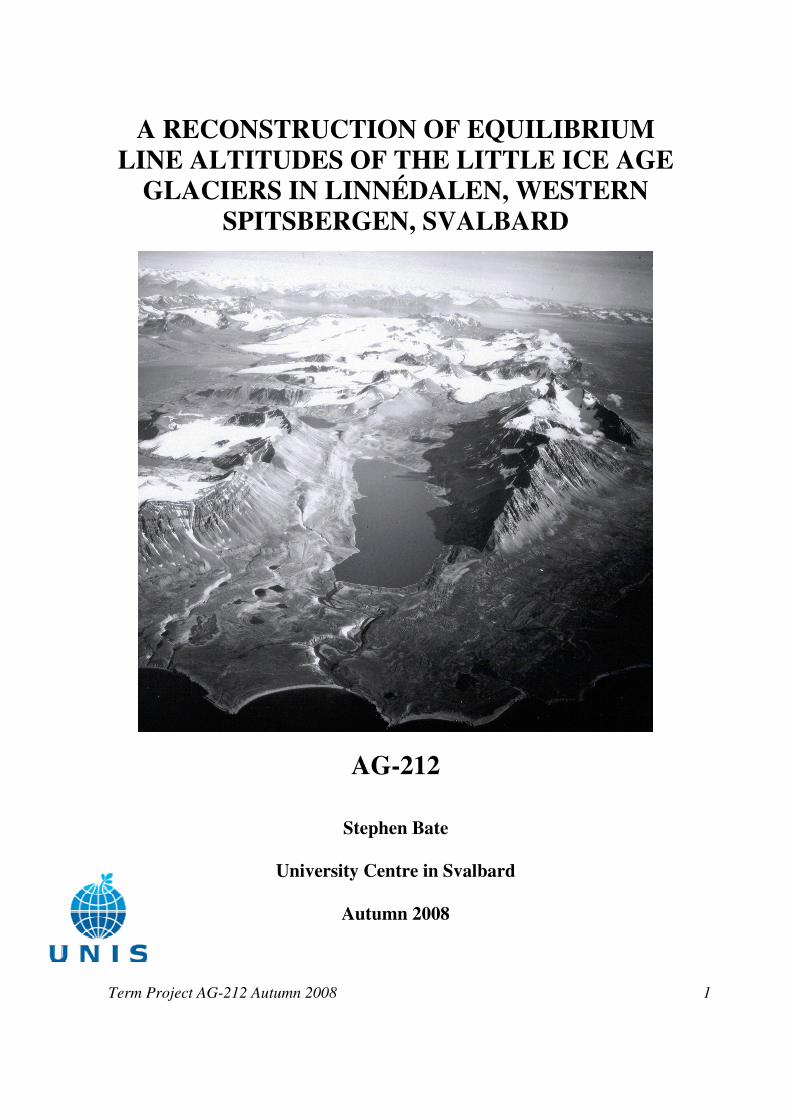
Term Project AG-212 Autumn 2008 1
A RECONSTRUCTION OF EQUILIBRIUM LINE ALTITUDES OF THE LITTLE ICE AGE
GLACIERS IN LINNÉDALEN, WESTERN SPITSBERGEN, SVALBARD
AG-212
Stephen Bate
University Centre in Svalbard
Autumn 2008

Term Project AG-212 Autumn 2008 2
A Reconstruction of Equilibrium Line Altitudes of the Little Ice Age Glaciers in Linnédalen, Western
Spitsbergen, Svalbard
Stephen Bate University Centre in Svalbard
Autumn 2008
ABSTRACT
Field altimetry and map based reconstruction techniques are used to hesitantly provide
Little Ice Age (LIA) equilibrium line altitudes (ELAs) in eight investigated cirques in
Linnédalen, western Spitsbergen, Svalbard. A LIA ELA of circa 200 metres (m) above
sea level (a.s.l.) to 300 m a.s.l. was found for the valley region. Lower ELAs were found
to the north of the study area, suggesting snowdrift ablation and accumulation had a
significant impact on the cirques. Furthermore, from comparison with field altimetry
measurements and from their small scale, it is advised that serious care has to be taken in
using Norsk Polarinstitutt (2008) 1:100,000 maps for ELA reconstruction.
1 INTRODUCTION
1.1 The LIA
The LIA was a widespread climatic cooling event that lasted from approximately the 14th
Century to the 19th
Century (Grove, 1988; Ogilvie and Jónsson, 2001). In the Northern
Hemisphere, a temperature decline from modern normals of between 0.6°C and 2oC was
experienced (Mann et al., 1999; Grove, 2004).
The Svalbard archipelago is situated in the High-Arctic between the latitudes of 76o and
81o north. On western Spitsbergen, the main island of the Svalbard archipelago, it has
been inferred that glaciers generally reached their LIA maximum around 1900 A.D.
(Hagen and Liestøl, 1990; Lefauconnier and Hagen, 1990) to 1936 (Mangerud and
Landvik, 2007), significantly later than regions at a lower latitude. It is a widespread
belief that the LIA represents the most extensive period of Holocene glacial advance on
Svalbard, as there are few Holocene ice marginal features that exist beyond LIA moraine
sequences (Kristiansen and Sollid, 1987; Mangerud et al., 1992; Werner, 1993; Svendsen
and Mangerud, 1997; Snyder et al., 2000).
Fleming et al. (1997) remark that whereas the potential importance of glaciers to
greenhouse-induced warming has been discussed by several authors (Meier, 1984; Meier,
Term Project AG-212 Autumn 2008 3
1990; Oerlemans and Fortuin, 1992), the reconstruction of High-Arctic glaciers has
seldom been performed, particularly on Svalbard (Fleming et al., 1997). This study will
therefore attempt to provide reconstructions of the size of LIA glaciers by establishing the
palaeo ELA of eight cirque glaciers in and around Linnédalen, western Spitsbergen.
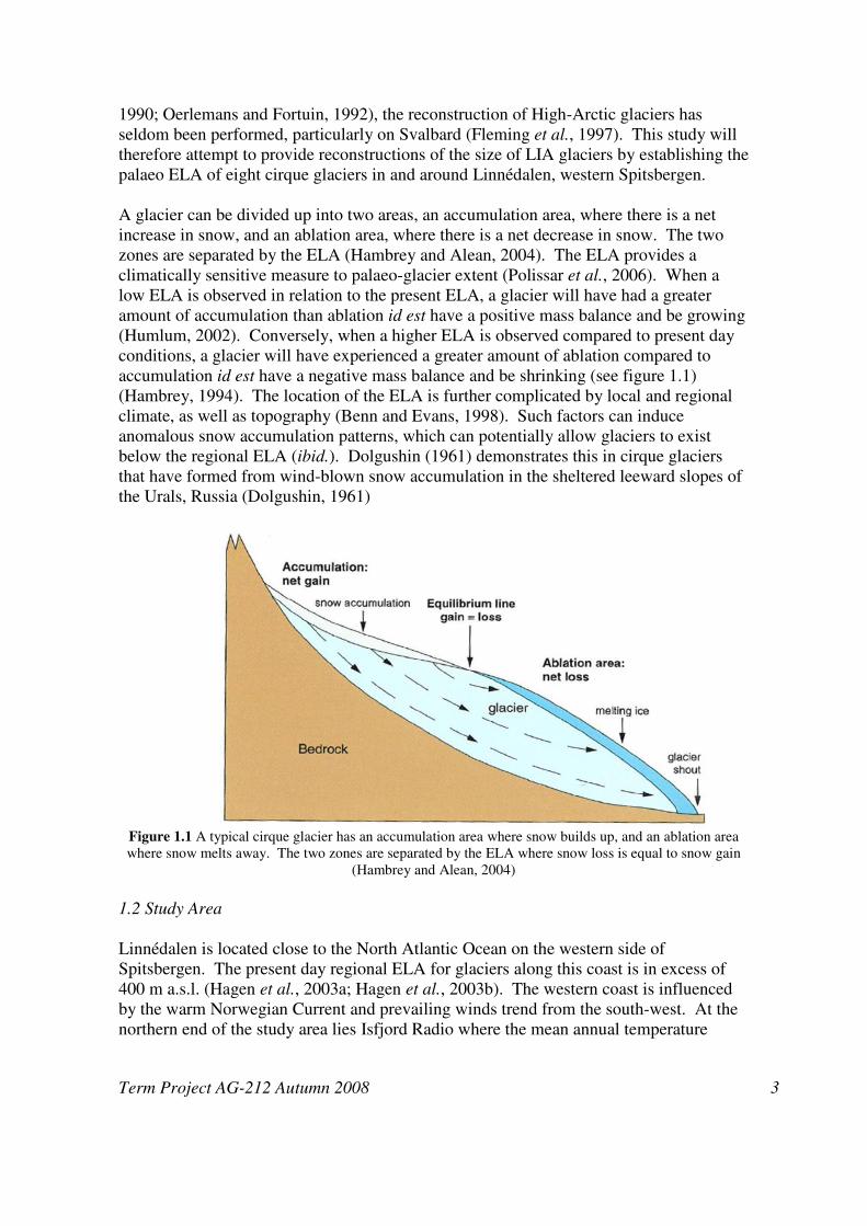
A glacier can be divided up into two areas, an accumulation area, where there is a net
increase in snow, and an ablation area, where there is a net decrease in snow. The two
zones are separated by the ELA (Hambrey and Alean, 2004). The ELA provides a
climatically sensitive measure to palaeo-glacier extent (Polissar et al., 2006). When a
low ELA is observed in relation to the present ELA, a glacier will have had a greater
amount of accumulation than ablation id est have a positive mass balance and be growing
(Humlum, 2002). Conversely, when a higher ELA is observed compared to present day
conditions, a glacier will have experienced a greater amount of ablation compared to
accumulation id est have a negative mass balance and be shrinking (see figure 1.1)
(Hambrey, 1994). The location of the ELA is further complicated by local and regional
climate, as well as topography (Benn and Evans, 1998). Such factors can induce
anomalous snow accumulation patterns, which can potentially allow glaciers to exist
below the regional ELA (ibid.). Dolgushin (1961) demonstrates this in cirque glaciers
that have formed from wind-blown snow accumulation in the sheltered leeward slopes of
the Urals, Russia (Dolgushin, 1961)
Figure 1.1 A typical cirque glacier has an accumulation area where snow builds up, and an ablation area
where snow melts away. The two zones are separated by the ELA where snow loss is equal to snow gain
(Hambrey and Alean, 2004)
1.2 Study Area
Linnédalen is located close to the North Atlantic Ocean on the western side of
Spitsbergen. The present day regional ELA for glaciers along this coast is in excess of
400 m a.s.l. (Hagen et al., 2003a; Hagen et al., 2003b). The western coast is influenced
by the warm Norwegian Current and prevailing winds trend from the south-west. At the
northern end of the study area lies Isfjord Radio where the mean annual temperature

Term Project AG-212 Autumn 2008 4
(1961-1990) is -5.1oC (Førland et al., 1997). The average temperatures in the coldest and
warmest months of the year are -12.4oC and +4.8
oC respectively (Mangerud and Landvik,
2007). Figure 1.2 illustrates the location of Linnédalen in the context of Svalbard and
further depicts the cirques that will make up the study sites of this paper. These sites
were largely chosen for their accessibility and from the presence of moraine sequences
illustrated on topographical maps.

Term Project AG-212 Autumn 2008 5
Figure 1.2 a) Map depicting the location of Linnédalen on the West coast of Spitsbergen, Svalbard
(modified from Norsk Polarinstitutt, 2000). b) Topographical map of Linnédalen depicting the eight areas
studied, labelled a-h: a) Grieg Cirque; b) Aagaard Cirque; c) Solryggen North Cirque; d) Solryggen South
Cirque; e) Solfonna Cirque; f) Linnébreen; g) Hermod Petersen Cirque; h) Kongress Cirque (modified from
Norsk Polarinstiutt, 2008a; Norsk Polarinstiutt, 2008b)
b)
Linnédalen
a)

Term Project AG-212 Autumn 2008 6
2. METHODOLOGY
2.1 ELA Reconstruction Using Geomorphological and Map Based Techniques
Several different methods have commonly been employed to determine estimated palaeo-
ELAs. The methods vary in their approach and all have some limitation or potential for
error (Porter, 2001). Nevertheless, the techniques are still utilised as they can provide a
very good proxy for past glacier size. Four different ELA reconstruction methods will be
used in this investigation.
2.2 Maximum Elevation of Lateral Moraines (MELM)
The MELM technique works on the premise that glacier flow results in a net transport of
debris from a glacier’s accumulation area to its ablation area (Benn and Evans, 1998). In
the ablation zone this debris is deposited as moraine sequences. As lateral moraines are
only deposited below the ELA, the method works on the idea that the uppermost altitude
of an abandoned lateral moraine marks the palaeo-ELA (Andrews, 1975; Nesje and Dahl,
2000).
Figure 2.1 The MELM ELA reconstruction technique works on the principle that the palaeo-ELA can be
estimated by measuring the altitude of the highest part of a glacier’s lateral moraine, as lateral moraines are
only deposited below the ELA (Porter, 2001)
There are some shortcomings with the MELM method however. The assumption has to
be made that deposition started at exactly the ELA but this may not always be the case,
which would lead to a lower observed ELA than was the case (Nesje and Dahl, 2000). In
addition, on steep slopes lateral moraines are often removed via mass movement and
erosional processes after ice retreat (Meierding, 1982). In such a situation the MELM
approach is likely to underestimate the ELA (Refsnider et al., 2007). What is more, ice
cored lateral moraines will likely experience a down-wasting effect after glacier retreat,
whilst lateral moraines in general will degrade post glaciation (Benn and Evans, 1998).
Such an occurrence would cause a speciously low ELA estimation. Conversely, if glacier
retreat is slow, then continued deposition from the glacier will result in a higher ELA
measurement (ibid.). Furthermore, continued deposition may occur on top of the lateral
moraines from steep valley sides, again leading to an overestimation in the height of the
ELA.
In this investigation lateral moraine height will be measured using an altimeter to the
nearest 0.5 m on both sides of the cirque. The highest lateral moraine will then be taken
as the ELA. The altimeter will be set to a fixed point at the start of each measurement
sequence and a final reading will be taken at the end of a day’s recordings from the same

Term Project AG-212 Autumn 2008 7
fixed point. Linnévatnet will provide the fixed point for measurements on Grieg cirque,
Aagaard cirque, Solryggen North cirque, Solryggen South cirque, Linnébreen and
Hermod Petersen cirque. Isfjorden will provide the fixed altitude for measurements taken
on Solfonna, whilst Kongressvatnet will provide the fixed altitude for measurements on
Kongress cirque. Wherever an altimeter reading is taken, the time and the temperature
will be recorded. After data collection, corrections will be made for temperature and
pressure throughout the sequence of readings. Pressure data for these corrections will be
taken from an automatic weather station deployed in the centre of Linnédalen,
approximately 750 m south of Linnévatnet.
2.3 Toe-to-Headwall Altitude Ratio (THAR)
The THAR works by setting the ELA at a fixed ratio between the toe of the former
glacier, construed from end moraine sequences, and the top of the valley headwall
(Leonard and Fountain, 2003). Figure 2.2 depicts the ELA on an exemplar cirque glacier
and demonstrates the equation used to calculate the ELA. Cirque and valley glaciers
often have a THAR of 0.35 to 0.40 and accordingly this investigation will calculate
THAR palaeo-ELAs using ratios of 0.35 and 0.4 (Meierding, 1982; Murray and Locke,
1989).
a) b)
ELA = At + THAR (Ah – At)
Figure 2.2 a) Diagram of the THAR ELA reconstruction method where Ah represents the headwall altitude
and At represents the glacier-toe altitude (Porter, 2001). b) Equation used to calculate the palaeo-ELA
A major problem exists in where to define the headwall limit of a former glacier and this
is a very subjective part of the assessment (Nesje and Dahl, 2000; Porter, 2001). Porter
(2001) comments how a high, steep headwall can provide a range of ELA estimates that
differ by 10s metres (m) to 100s m (Porter, 2001). The THAR method is widely regarded
as the crudest of the four methods that will be employed in this survey, as it takes no
account of glacier hypsometry or climatic considerations (Benn and Evans, 1998).
Nevertheless, it provides a simple and relatively rapid means of past ELA assessment.
In this study, glacier toe heights will be measured in the field using the same altimetry
methods outlined in the MELM section above. Again these altimetry values will be
corrected for temperature and pressure. Headwall values will be taken from Norsk
Polarinstitutt (2008a; 2008b) 1:100,000 topographical maps (Norsk Polarinstiutt, 2008a;
Norsk Polarinstiutt, 2008b). Ideal topographic maps would provide contours at 30 m or
less (Porter, 2001). The maps available for Svalbard provide contours only at 50 m
intervals, and as such, a certain amount of interpolation will be required.

Term Project AG-212 Autumn 2008 8
2.4 Accumulation Area Ratio (AAR)
The AAR method is based on the assumption that the accumulation area of a glacier
occupies a fixed proportion of the total glacier area (Benn and Gemmell, 1997).
Empirical studies of modern glaciers have shown that under steady-state conditions, an
AAR of 0.6 can be assumed to characterise cirque glaciers (Meier and Post, 1962; Porter,
1975; Porter, 1977; Kuhn, 1989; Benn and Evans, 1998; Benn and Lehmkuhl, 2000;
Nesje and Dahl, 2000; Porter, 2001; Rea and Evans, 2007). The methodology starts with
the mapping of a glacier’s extent on a topographical map using glacial and
geomorphological observations, for instance lateral and end moraines, erratics and
trimlines (Porter, 1981). An estimated initial ELA is applied to this palaeo-glacier outline
from which contours of the glacier surface are applied in accordance with the
topographical map. Below the estimated ELA, glacier contours are convex and above the
ELA the contours are concave consistent with glacier flow patterns. The degree of
concavity and convexity should increase with distance from the ELA (figure 2.3) (Porter,
2001). The area between each contour can then be used to produce a graphical
representation of the glacier’s area/altitude distribution, which can then be used to satisfy
an AAR of 0.6 (ibid.).
a)
b)
Figure 2.3 a) Method of reconstructing an ELA using the AAR approach, where Sc represents the
accumulation area and Sa represents the ablation area (Porter, 2001). b) Equation that has to be satisfied
for a cirque glacier with an assumed AAR of 0.6
The largest source of error associated with this method is the reconstruction of glacier
surface contours. Nevertheless, this source of inaccuracy is considered to be randomly
distributed and is not considered to introduce major deviations (Nesje and Dahl, 2000).
Additionally, the palaeo-glacier extent is a somewhat subjective operation. Another
shortcoming of the AAR reconstruction technique is that little account of glacier area
over its altitudinal range is considered (Furbish and Andrews, 1984). Further, Benn and
Evans (1998) comment how former glacier ELAs based on a uniformly assumed AAR
value may be subject to significant errors if there is a wide range of glacier shapes in the
study area (Benn and Evans, 1998).
In this study the ELA estimation will come from map based calculations with palaeo-
glacier extent configured from field observations, aerial photography and topographic
maps of Linnédalen. Norsk Polarinstitutt (2008a; 2008b) 1:100,000 topographical maps
will be computer enhanced to a larger scale and then printed onto 2 millimetre (mm)
square paper (Norsk Polarinstiutt, 2008a; Norsk Polarinstiutt, 2008b). From this, the

Term Project AG-212 Autumn 2008 9
procedure outlined above will then be carried out until an ELA estimation is calculated.
Surface debris in the ablation zone can modify the AAR, however field observations and
oblique aerial photographs from 1936 would suggest that this was not the case
(Mackintosh et al., 2006).
2.5 Balance Ratio (BR)
The BR method takes account of the deficiencies of the AAR approach in that it
considers glacier hypsometry. It works on the principle that, for a glacier in state of
equilibrium, the total annual accumulation above the ELA must balance that of the total
ablation below the ELA (Furbish and Andrews, 1984; Benn and Evans, 1998; Nesje and
Dahl, 2000; Rea and Evans, 2007). It further differs from the AAR approach in that it
considers glacial area within each altitudinal contour band (Mark and Helmens, 2005).
For this particular investigation, a BR computerised spreadsheet will be used to
reconstruct the palaeo-ELAs for Linnédalen. The spreadsheet is a modified version of
that produced by Benn and Gemmell (1997). Contour intervals will be set at 50 m and,
for ease and consistency, the same palaeo-glacier reconstructions used in the AAR
assessment will be used and thus the same areas calculated using the technique described
in section 2.4 will be applied.
2.6 Aerial Photography
Aerial photographs exist of Linnédalen from 1936, 1961, 1969, 1990 and 1995. The plan
view photographs from 1961, 1969, 1990 and 1995 were taken in mid-August of their
respective year, which can be assumed to be at or very close to the end of the ablation
season for Svalbard. The pictorial representation of Linnédalen from these four years
will provide additional help in the establishment of the location of the MELM before
field observations take place. Moreover, they will provide guidance for the AAR and BR
palaeo-ELA reconstruction approaches. The 1936 photographs are oblique and are of
less use than the plan view photographs.
2.7 Chronology
Evidence for LIA cirque glacier advances in Linnédalen comes largely from unweathered
moraines. Due to the nature of the bedrock geology in the valley, other glacial landforms
are sparse. The moraines have been correlated to the LIA from the use of aerial
photographs from 1936 taken by the Norsk Polarinstitutt.

Term Project AG-212 Autumn 2008 10
3. RESULTS
Field altimetry data were collected from the eight study sites. This was then corrected for
temperature and pressure, and any repeat measurements were averaged together. The
highest MELM for each study site was then compiled together to form the MELM
estimated ELA. The map-based reconstructions were further assembled together and a
mean result of all five estimations was produced for each site. No weighting was made in
favour of any one method. All the results are presented in table 3.1.
Reconstructed Equilibrium Line Altitude (m a.s.l.)
Cirque Name MELM THAR (0.4) THAR (0.35) AAR (0.6) BR Mean Grieg Cirque 121 245 225 195 221 197
Aagaard Cirque 214 200 185 245 248 200
Solryggen North Cirque 262 285 275 280 310 274
Solryggen South Cirque 250 305 290 315 331 282
Solfonna Cirque 214 380 350 285 341 315
Linnébreen 270 285 260 290 305 272
Hermod Petersen Cirque 219 300 285 320 332 268
Kongress Cirque 228 215 210 230 242 218
Table 3.1 The reconstructed ELAs of the eight investigated cirques in the Linnédalen area using the
MELM, THAR (0.4), THAR (0.35), AAR (0.6) and BR approaches
Using the data from table 3.1, the author hesitantly suggests a mean LIA ELA between
200 m a.s.l. and 300 m a.s.l. in Linnédalen, with the average mean ELA in the study
region equalling 253 m a.s.l.. In addition, there appears to be a lowering of ELAs in the
north compared with the south of the region. Data show that the BR method generally
produces the highest ELAs. On the whole, the MELM method produces the lowest ELA
estimates, closely followed by the THAR (0.35) technique. Places that consistenantly
produced low ELAs include Grieg cirque, Aagaard cirque and Kongress cirque. These
cirques trend around 50 m lower than the remaining five studied cirques. Furthermore, in
looking at the three closest cirques, Solryggen North, Solryggen South and Solfonna, the
estimates depict a higher palaeo-ELA on the west of Linnéfjella. Nevertheless in making
these comparisons, it may be that one or two exceptionally high reconstructions may be
skewing the mean ELA away from that recorded in the field. Indeed, the MELM
approach for Solfonna produces a 100 m lower ELA estimation than the mean ELA
would suggest and a difference between the highest estimate and lowest estimate of 166
m. In addition, Grieg and Hermod Petersen produce results that have a range of over 100
m. The most comparable data series are found at Kongress (35 m difference in results),
Linnébreen (45 m difference in results) and Solryggen North (48 m difference in results).

Term Project AG-212 Autumn 2008 11
4. DISCUSSION
4.1 Interpretation of LIA ELAs
The results collected in this investigation indicate a LIA ELA lower than at present,
indicating colder conditions and therefore an increase in snow accumulation, from
increased precipitation and/or reduced ablation during the LIA. The potential for higher
ELAs at Solfonna, Solryggen South and Solryggen North may be the result of the
prevailing south-westerly winds that blew through Tjørnskaret. In the field, it was
observed to be one of the windiest places in the study area, and the author speculates that
the pass may have had a tunnelling effect. This would have exacerbated the effects of
snowdrift at these study sites, increasing ablation. Further, it would explain why
Linnébreen and Hermod Petersen cirque were impacted less, due to being further away
from the Tjørnskaret wind tunnelling effect and from the shelter that they would have
received from their own local topographical features. Despite being potentially more
exposed to the prevailing wind on the west of Linnéfjella, which might explain the higher
ELA here, the author proposes that ice was still able to accumulate in Solfonna due to a
north westerly trending valley (figure 4.1).
Figure 4.1 The importance of topography for either raising or lowering ELAs is demonstrated here. The
abbreviation TPW-ELA stands for temperature, precipitation and wind equilibrium line altitude. The
abbreviation TP-ELA stands for temperature and precipitation equilibrium line altitude. Prevailing wind on
western Spitsbergen is from the south-west. In the study area it is hypothesised that Tjørnskaret would
have acted as a wind tunnel that would have effectively raised ELAs of Solfonna cirque, Solryggen South
and Solryggen North. Further north in the Grieg cirque and Aagaard cirque, it is conjectured that
Linnéfjella provided enough shelter to lower ELAs through the positive accumulation of snowdrift
(modified from Dahl et al., 2003)
Approximately 1.5 kilometres (km) north of Grieg cirque, another potential LIA cirque
was identified and investigated with the idea of establishing a LIA ELA. It was decided

Term Project AG-212 Autumn 2008 12
that the investigated hollow was not a cirque glacier however, and was more likely a
glacieret, a thin ice patch where accumulation may not have quite reached high enough
levels to flow out of the cirque. It is possible that glacier motion may have once been
initiated as the snow patch extended over 30 m from the base of its back wall. At such a
distance forces imposed by weight and surface gradient overcome internal resistance and
the ice can move (Ballantyne and Benn, 1994). Nevertheless, no discernable moraine
features were found and the glacieret was likely formed by snow drift and avalanches,
assisted by topographic shelter from Linnéfjella.
The LIA ELA of the Grieg cirque can be compared to that of Snyder et al. (2000) whom
used the AAR methodology. Using a value of 0.6 they produced an ELA of between 230
and 280 m a.s.l. (Snyder et al., 2000). This value provides a higher LIA ELA than the
same AAR reconstruction in this paper, and further a higher LIA ELA than the mean
altitude. The author attributes this difference to the subjective nature in the AAR
technique, something which is not assisted by the small scale topographic maps available
for reconstruction exercises on Svalbard. Mangerud and Svendsen (1990) produced an
ELA estimate of between 250 m and 300 m for Linnébreen (Mangerud and Svendsen,
1990). From the assumption that their established heights, as well as the palaeo-ELAs
presented in this study, are accurate, it would suggest a rise of some 10s m has occurred
in the ELA during the past eighty years. This statement is supported by Snyder et al.
(2000). In contrast, in north-west Spitsbergen around Kongsfjorden, a 100 m lowering of
ELAs during the LIA has been reported compared to today (Liestøl, 1988). This would
indicate that greater warming and/or a decrease in the accumulation of snowfall has been
experienced since the end of the LIA in Kongsfjorden.
4.2. Methodology Review
As was suggested in the methodology there are inherent problems with all of the ELA
reconstruction techniques. Firstly, map based reconstruction techniques, namely THAR,
AAR and BR are a subjective assessment. For the THAR method, both the headwall and
toe altitudes have to be estimated, whilst with the AAR and BR reconstructions the entire
area of the palaeo-glacier has to be predicted. This is further complicated by the small
scale maps available for Svalbard where contours are set at 50 m. This requires a certain
level of interpolation and as such values will vary for each individual’s reconstruction
depending on their own interpretation of the topographic maps. The small scale maps
will thus generate greater variation in ELA estimates for small differences in either
chosen toe and headwall values or in palaeo-glacier area. The author proposes these
factors in the difference between the results presented for Grieg cirque in this paper and
in Snyder et al. (2000).
The MELM approach is also potentially flawed. Problems were experienced in the field
in the determination of the exact upper limit of the lateral moraine. Aerial photography
assisted greatly with this problem, nevertheless, it is high plausible that someone
repeating this study may produce ELA estimates 10s m different to results printed here.
Furthermore, the predominant underlying geology of Linnéfjella is highly erodible
phyllite, and being so highly erodible, it was often difficult to distinguish between the

Term Project AG-212 Autumn 2008 13
upper limit of a lateral moraine and skree or weathered bedrock (Snyder et al., 2000).
Lateral moraines had also to contend with steep valley sides in several of the cirques,
which may have led to an underestimation in the ELA. Additionally, some of the lateral
moraines had been eroded and it is almost certain that all of the lateral moraines will have
experienced some amount of downwasting since the end of the LIA. This in part would
help to explain the much lower ELA values produced using this method. If MELM ELA
figures were used on their own, it would suggest that the LIA ELAs in the investigated
area were between 30 m and 80 m lower than late 20th
Century ELAs in the region.
It should be noted that altimetry values were produced by the use of a handheld altimeter.
This was because a Global Positioning System (GPS) could not pick up enough satellites
at such a high latitude in order to provide accurate altitude readings. The human error in
the use of a handheld altimeter is considered to have only a negligible impact upon
results. It is for this reason, combined with the small scale maps available for the
Linnédalen region, that toe readings were taken using the altimeter. By combining map
and field data there is a greater potential for error, yet end moraine sequences tend to be
deposited on relatively flat topography, reducing the significance somewhat. Indeed,
altimeter heights were chosen for use because they could potentially provide a more
detailed ELA reconstruction than map based reconstruction alone. Further, it was
considered much easier to establish where the glacier toe was in the field than on a map.
Despite the flaws in all of the ELA reconstruction approaches, the author largely
considers the MELM procedure to be the most effective for use on Svalbard because of
the small scale of topographic maps available. Additionally, despite producing lower
ELA estimates from the down wasting of ice cored moraines, the MELM approach
provides the most precise palaeo-ELA estimate compared with the THAR, AAR and BR
techniques for Linnédalen. So long as one of the two lateral moraines can be found for
assessment that has not been: deposited on a steep slope; has had material added to it by
debris after deposition; had a palaeo-glacier that experienced periods of re-advance in a
time of generalised retreat; or been extensively eroded, then a slightly lowered, but
nonetheless reliable, past ELA can be established.
4.3 The Value of Field and Aerial Photography in the MELM Approach
MELM ELA estimates were considerably assisted by field photography and aerial
photography. Having a plan view of a study area provided by aerial photography was a
real help in this investigation. Seeing things on the ground when a scientist is right in the
middle of what they are looking at is often very difficult, so having an initial idea of
conditions in a cirque considerably abetted this investigation. In addition, when in the
field, there were occasions whereby taking a photograph of a cirque and using the zoom
function, features, for instance the continuation of a lateral moraine over 100s m, became
more prominent and easier to interpret. An example of this is shown in figure 4.2.

Term Project AG-212 Autumn 2008 14
Figure 4.2 Photography can greatly assist in field observations. Here, what is interpreted as a LIA lateral
moraine in the Solfonna cirque is highlighted, something that was not discernable from initial field
observations.
4.4. Norsk Polarinstitutt 1:100,000 Topographic Maps – A Comment
During the reproduction of LIA ELAs from the use of map based techniques, a marked
difference between certain field observations and the Norsk Polarinstitutt 1:100,000
topographic maps were noted. Several altimetry readings for toe and lateral moraines
were recorded at a sufficiently lower elevation than they appear on the maps. Examples
of this can be found at Kongress cirque where from the topographic maps, a toe estimate
would be approximately 25 m to 50 m higher than what was recorded in the field. In
addition, in Hermod Petersen cirque, moraine sequences stretch from below 200 m to
above 300 m, whereas from field altimetry the toe was recorded at 185m with the highest
discernable LIA moraine being located at 219m. This illustrates another problem when
using small scale topographic maps to reproduce LIA ELAs. It may be possible that what
has been inferred as moraine is in fact the product of mass movement processes. Further,
the Norsk Polarinstitutt provide no age constraint to any moraine formations, and so
scientists who wish to produce LIA ELA estimates have to assume that all moraine from
previous glacial advances has been overridden by LIA glaciers. Nevertheless, there is the
possibility that, due to Svalbard’s inaccessible nature, mapping errors have occurred.
This is a serious consideration, in that the Norsk Polarinstitutt (2008) maps have been
produced predominantly using aerial photographs from 1990 and 1995, as well as glacier
fronts at sea level being produced by Landsat images from 1998. The issue of glacier
retreat was recorded in the field at Solfonna cirque, for example, where an anticipated 2.5
km glacier had retreated beyond recognition from the map (figure 4.3). The fact that
many of these cirques are now, or are virtually, ice free, supports Snyder et al. (2000)
statement that there exists a sensitive threshold on ice accumulation in the cirques of

Term Project AG-212 Autumn 2008 15
Linnédalen. What impact such climatic sensitivity may have on the larger glaciers of
western Spitsbergen is not the premise of this paper, however.
Figure 4.3 A photograph of Solfonna cirque trending up cirque (south-east). A rapid decline in the glacier
can be seen compared to the level of ice expected from the Norsk Polarinstitutt (2008b) 1:100,000
topographic map (for an indication of expected ice see figure 1.2 b).
4.5 Future Work
This project lends itself to several potential avenues of future work. In terms of field
observations and the MELM technique, it would be of interest to compare to the cirques
of Linnédalen with other cirques along the west coast, form both lower and higher
latitudes. Present day western coast ELAs differ quite considerably, being higher in
north-west coastal localities than in south-west coastal regions (Hagen et al., 2003a;
Hagen et al., 2003b). Moreover, within the vicinity of Linnédalen, the west Grønfjorden
region appears to hold several cirque glaciers that would seem to have LIA moraine
sequences. What is more, it would be interesting to model the LIA ELAs from west
Spitsbergen to east Spitsbergen to measure any potential rise in localised ELA. This rise
would be anticipated due to a decrease in distance from the main direct precipitation
source (the North Atlantic) and hence the author would anticipate a fall in precipitation,
parallel with that experienced on Svalbard today (Humlum, 2002).
In terms of future work on topographic map based LIA ELA reconstructions, a
refinement of previous glacier extent in Linnédalen region could be readily achieved.
Furthermore, constraints on the Benn and Gemmell (1997) spreadsheet used to calculate
the BR ELA estimate would potentially combat ELA overestimation for the western
Svalbard region.

Term Project AG-212 Autumn 2008 16
5. CONCLUSSION
• Averaged reconstructions in Linnédalen region suggest a LIA ELA of between 200 m
a.s.l. and 300 m a.s.l.. This is approximately 100 m to 200 m or more lower than the
western coast of Spitsbergen at present (Hagen et al., 2003a; Hagen et al., 2003b).
There appears to be a lowering in the ELA in the north of the valley compared to the
south, which may be the result of Tjørnskaret acting as a wind tunnel and
exacerbating the impact of snowdrift ablation around Solfonna, Solryggen North and
Solryggen South. Glaciers further north would receive greater protection from
Linnéfjella against snowdrift ablation and may in fact benefit from the positive
accumulation of snowdrift.
• Care has to be taken in using reconstruction techniques that rely on topographic maps
in places, such as Svalbard, where only small scale maps are available. Potential
problems can also arise from using the MELM technique because of down-wasting of
ice cored moraines and from the difficulty in discerning where ELAs reach their
maximum, either from slow glacier retreat or from the product of erosional and mass
movement activity in steep sided cirques.
• Despite producing a lower ELA estimate for LIA glaciers, it is the opinion of the
author that the MELM approach to ELA reconstruction engenders the most accurate
estimations in Svalbard. This is due to the small scale, as well as possible
inaccuracies contained within, the Norsk Polarinstitutt (2008) maps that have largely
been produced on the basis of aerial photographs from 1990 and 1995, with glacier
fronts mapped using Landsat images from 1998.
ACKNOWLEDGEMENTS
The original field data presented in this written work was collected between 22nd
July
2008 and 10th
August 2008 as part of an International Polar Year (IPY) joint
collaboration between the United States National Science Foundation (US NSF) Research
Experience for Undergraduates (REU) programme and the University Centre in Svalbard
(UNIS) Arctic Geology 212 course, ‘Holocene and Modern Climate Change in the High
Arctic, Svalbard’.
The author of this paper wishes to foremost thank Mike Retelle for the inspiration to
undertake this project and for the invaluable advice he bestowed both in and out of the
field. Further, to all the REU/UNIS students and associates, in particular Maya Wei-
Haas, Leo Sold and Anthony Novak, for their helpful work, advice and companionship in
the field. Logistical support was provided by UNIS, US NSF REU programme and
Isfjord Radio. A final thanks should go to everyone at Isfjord Radio, who were so
understanding to our needs and made this field season so much more pleasant.
REFERENCES
Andrews, J.T. (1975) Glacial Systems: An Approach to Glaciers and their Environments.
North Scituate, Massachusetts: Duxbury Press

Term Project AG-212 Autumn 2008 17
Ballantyne, C.K., Benn, D.I. (1994) ‘Glaciological Constraints on Protalus Rampart
Development’. Permafrost and Periglacial Processes 5, 145-153
Benn, D.I., Gemmell, A.M.D. (1997) ‘Calculating Equilibrium Line Altitudes of Former
Glaciers by the Balance Ratio Method: A New Computer Spreadsheet’. Glacial Geology
and Geomorphology (http://ggg.qub.ac.uk/papers/full/1997/tn011997/tn01.html)
Benn, D.I., Evans D.J.A. (1998) Glaciers and Glaciations. London: Arnold
Benn, D.I., Lehmkuhl, F. (2000) ‘Mass Balance and Equilibrium-Line Altitudes of
Glaciers in High-Mountain Environments’. Quaternary International 65/66, 15–29
Dahl S.O., Bakke J., Lie O., Nesje A. (2003) ‘Reconstruction of Former Glacier
Equilibrium-Line Altitudes Based on Proglacial Sites: An Evaluation of Approaches and
Selection of Sites’. Quaternary Science Reviews 22(2), 275-287
Dolgushin, L.D. (1961) ‘Main Features of the Modern Glaciation of the Urals’. IASH 54,
335-347
Fleming, K.M., Dowdeswell, J.A., Oerlemans, J. (1997) ‘Modelling the Mass Balance of
Northwest Spitsbergen Glaciers and Responses to Climate Change’. Annals of
Glaciology 24, 203-210
Førland, E., Hanssen-Bauer, I., Nordli, P. (1997) ‘Climate Statistics and Longterm Series
of Temperatures and Precipitation at Svalbard and Jan Mayen’. Norwegian
Meteorological Institute, Report 21/97, 1-72
Furbish, D.J., Andrews, J.T. (1984) ‘The Use of Hypsometry to Indicate Long-term
Stability and Response of Valley Glaciers to Changes in Mass Transfer’. Journal of
Glaciology 30, 199–211
Grove, J.M. (1988) The Little Ice Age. London: Methuen
Grove, J.M. (2004) Little Ice Ages: Ancient and Modern. London: Routledge
Hagen, J., Liestøl, O. (1990) ‘Long-Term Glacier Mass-Balance Investigations in
Svalbard’. Annals of Glaciology 14, 102-106
Hagen, J.O., Kohler, J., Melvold, K., Winther, J.G. (2003a) ‘Glaciers in Svalbard: Mass
Balance, Runoff and Freshwater Flux’. Polar Research 22, 145-159
Hagen, J., Melvold, K., Pinglot, F., Dowdeswell, J. (2003b) ‘On the Net Mass Balance of
the Glaciers and Ice Caps in Svalbard, Norwegian Arctic’. Arctic Antarctic and Alpine
Research 35, 264-270
Hambrey, M. (1994) Glacial Environments. London: CRC Press
Hambrey, M., Alean, J. (2004) Glaciers. Cambridge: Cambridge University Press
Kristiansen, K.J., Sollid, J.L. (1987) ‘Svalbard, Jordartskart 1:1,000,000. Nasjonalatlas
for Norge’. Geografisk Institutt, Univeritet i Oslo
Humlum, O. (2002) ‘Modelling Late 20th
-Century Precipitation in Nordenskiöld Land,
Svalbard, by Geomorphic Means’. Norsk Geografisk Tidsskrift 56, 96-103
Kuhn, M. (1989) ‘The Response of the Equilibrium Line to Climate Fluctuations: Theory
and Observations’. In Glacier Fluctuations and Climate Change Oerlemans, J. (ed.),
407–417. Dordrecht: Kluwer
Lefauconnier, B., Hagen, J. (1990) ‘Glaciers and Climate in Svalbard: Statistical Analysis
and Reconstruction of the Brøggerbreen Mass Balance for the Last 77 Years’. Annals of
Glaciology 14, 148-152
Leonard, K.C., Fountain, A.G. (2003) ‘Map-Based Methods for Estimating Glacier
Equilibrium-Line Altitudes’. Journal of Glaciology 49(166), 329-336

Term Project AG-212 Autumn 2008 18
Liestøl, O. (1988) ‘The Glaciers of the Kongsfjorden Area, Spitsbergen’. Norsk
Geografisk Tidsskrift 42, 231–38
Mackintosh, A.N., Barrows, T.T., Colhoun, E.A., Fifield, L.K. (2006) ‘Exposure Dating
and Glacial Reconstruction at Mt. Field, Tasmania, Australia, Identifies MIS 3 and MIS 2
Glacial Advances and Climatic Variability’. Journal of Quaternary Science 21(4), 363–
376
Mangerud, J., Svendsen, J.I. (1990) ‘Deglaciation Chronology Inferred from Marine
Sediments in a Proglacial Lake Basin, Western Spitsbergen, Svalbard’. Boreas 19, 249–
72
Mangerud, J., Bolstad, M., Elgersma, A., Helliksen, D., Landvik, J.Y., Lønne, I., Lycke,
A.K., Salvigsen, O., Sandahl, T., Svendsen, J.I. (1992) ‘The Last Glacial Maximum on
Western Svalbard’. Quaternary Research 38, 1-31
Mangerud, J., Landvik, J.Y. (2007) ‘Younger Dryas Cirque Glaciers in Western
Spitsbergen: Smaller than During the Little Ice Age’. Boreas 36, 278-285
Mann, M. E., Bradley, R. S., Hughes, M. K. (1999) ‘Northern Hemisphere Temperatures
During the Past Millennium: Inferences, Uncertainties, and Limitations’. Geophysical
Research Letters 26, 759–762
Mark, B.G., Helmens, K.F. (2005) ‘Reconstruction of Glacier Equilibrium-Line Altitudes
for the Last Glacial Maximum on the High Plain of Bogotá, Eastern Cordillera,
Colombia: Climatic and Topographic Implications’. Journal of Quaternary Science
20(7–8), 789–800
Meier, M.F., Post, A.S. (1962) Recent Variations in Mass Net Budgets of Glaciers in
Western North America. International Association of Scientific Hydrology 58, 63-77
Meier, M.F. (1984) ‘Contribution of Small Glaciers to Global Sea Level’. Science
226(4681), 1418-1421
Meier, M.F. (1990) ‘Reduced Rise in Sea Level’. Nature 343(6254), 115-116
Meierding, T. C. (1982) ‘Late Pleistocene Glacial Equilibrium-Line Altitudes in the
Colorado Front Range: A Comparison of Methods’. Quaternary Research 18, 289–310
Murray, D.R., Locke, W.W.III (1989) ‘Dynamics of the Late Pleistocene Big Timber
Glacier, Crazy Mountains, Montana, U.S.A.’. Journal of Glaciology 35, 183–190
Nesje, A., Dahl, S.O. (2000) Glaciers and Environmental Change. New York: Oxford
University Press
Norsk Polarinstitutt (2000) Norsk Polarinstitutt website. Available at:
http://miljo.npolar.no/temakart/images/maps/GeneralMapOfSvalbardAndKeymap.gif
[Access date: 01 August 2008]
Norsk Polarinstitutt (2008a) Svalbard 1:100,000 series: B9 – Isfjorden. Tromsø: Norsk
Polarinstitutt
Norsk Polarinstitutt (2008a) Svalbard 1:100,000 series: B10 – Van Mijenfjorden.
Tromsø: Norsk Polarinstitutt
Oerlemans, J., Fortuin, J.P.F. (1992) ‘Sensitivity of Glaciers and Small Ice Caps to
Greenhouse Warming’. Science 258(5079), 115-117
Ogilvie, A.E.J., Jónsson, T. (2001) ‘“Little Ice Age” Research: A Perspective from
Iceland’. Climatic Change 48, 9-52
Polissar, P.J., Abbott, M.B., Wolfe, A.P., Bezada, M., Rull, V., Bradley, R.S (2006)
‘Solar Modulation of Little Ice Age Climate in the Tropical Andes’. Proceedings of the
National Academy of Sciences 103(24), 8937-8942

Term Project AG-212 Autumn 2008 19
Porter, S.C. (1975) ‘Equilibrium Line Altitudes of Quaternary Glaciers in the Southern
Alps, New Zealand’. Quaternary Research 5, 27–47
Porter, S.C. (1977) ‘Present and Past Glaciation Threshold in the Cascade Range,
Washington State, USE: Constraints Provided by Palaeoenvironmental Reconstructions’.
The Holocene 11, 607–611
Porter, S.C. (1981) ‘Glaciological Evidence of Holocene Climatic Change’. In Climate
and History Wigley, T.M.L., Ingram, M.J., Farmer, G. (eds.), 82-110. Cambridge:
Cambridge University Press
Porter, S.C. (2001) ‘Snowline Depression in the Tropics During the Last Glaciation’.
Quaternary Science Reviews 20, 1067-1091
Rea, B.R., Evans D.J.A. (2007) ‘Quantifying Climate and Glacier Mass Balance in North
Norway During the Younger Dryas’. Palaeogeography, Palaeoclimatology,
Palaeoecology 246, 307–330
Refsnider, K.A., Laabs, B.J.C., Mickelson, D.M. (2007) ‘Glacial Geology and
Equilibrium Line Altitude Reconstructions for the Provo River Drainage, Uinta
Mountains, Utah, U.S.A.’. Arctic, Antarctic and Alpine Research 39(4), 529–536
Snyder, J.A., Werner, A., Miller, G.H. (2000) ‘Holocene Cirque Glacier Activity in
Western Spitsbergen, Svalbard: Sediment Records from Proglacial Linnévatnet’. The
Holocene 10(5), 555-563
Svendsen, J.I., Mangerud, J. (1997) ‘Holocene Glacial and Climatic Variations on
Spitsbergen, Svalbard’. The Holocene 7(1), 45-57
Werner, A. (1993) Holocene Moraine Chronology, Spitsbergen, Svalbard: Lichenometric
Evidence for Multiple Neoglacial Advances in the Arctic. The Holocene 3, 128–37