a remote sensing application for image classification

A remote sensing application for image classification

using unsupervised methods

A Class Project

By

Mayuri Bhattacharyya

Advisor

Dr. Xin Maio

Department of Geography, Geology, and Planning

Missouri State University

Location:

The region is in the central east part of the state of Chihuahua in Mexico. This is a watershed

region bounded by two highlands of Mexico namely Sierra Bonce in the north and Sierra la

Gloria in the south. The name of the river is Sierra del Soldado which is one of the major streams

in Mexico.

This river is important in respect to the water distribution system with in Chihuahua in Mexico.

This river is the perennial, and meandering in its course. The above three maps are of Mexico,

Chihuahua State, and the study area, respectively. My current research is on this region’s images

which include a remote sensing application for image classification of the study area using

unsupervised methods.

The above images are the satellite imagery of the study area using TM (Thematic Map) bands.

The first image is a combination of three part of the same image. The first bigger part (Image

window) shows the main study area. The left side image with the black boundary (Scroll

window) shows the surrounding area in a broad way, and the right side small image (Zoom

window) shows the particular part of the image in a zooming layer. These images are the product

of the remote sensing software ESRI ENVI 4.2. The left side broad image is from the Google

earth software.

Hypothesis:

I have attempted to make a remote sensing application for image classification for the study area.

Why this effort is required because this region is neglected for the study of scientific research

due to its inaccessibility for the steep surface with the existence of

some dense forest. Therefore remote sensing applications should

be applied to study this region, to extract the thematic information

from the images, and to recognize the pattern of the bands in the

images. My research is going to prove if we follow the remote

sensing techniques we must be careful about the selection of the

classification methods because there might be some

misinterpretations, too. I am going to show use of unsupervised

approaches to classify the images of the study area. I have used TM images with three bands,

namely: Red (R) band 4, Green (G) band 3, and Blue (B) band 2.

Methods:

Classification of the images-

Now a day people generally rely on the multispectral classifications, algorithms based on

parametric and nonparametric statistics using either supervised or unsupervised logic. Parametric

methods such as maximum likelihood classification and unsupervised clustering assume

normally distributed remoter sensor data and knowledge about the forms of the underlying class

density functions. I have used here unsupervised classification methods to explore the spectral

characteristics.

Unsupervised Classification-

In an unsupervised classification, the identities of land-cover types to be specified as classes

within a scene are not generally known a priori because ground reference information is lacking

or surface features within the scene are not well defined. The computer is required to group

pixels with similar spectral characteristics into unique clusters according to some statistically

determined criteria. The analyst then re-labels and combines the spectral clusters into

information classes. This method is commonly referred to as clustering. This is an effective

method of partitioning remote sensor image data in multispectral feature space and extracting

land-cover information. Compared to supervised classification normally requires only a minimal

amount of initial input from the analyst. This is because clustering does not normally require

training data. This is the process where numerical operations are performed that search for

natural groupings of the spectral properties of pixels, as examined in multispectral feature space.

The clustering process results in a classification map consisting of m spectral classes. The analyst

then attempts a posteriori (after the fact) to assign or transform the spectral classes into thematic

information classes of interest like forest, agriculture, etc. This may be difficult. Some spectral

clusters may be meaningless because they represent mixed classes of Earth surface materials.

The analyst must understand the spectral characteristics of the terrain well enough to be able to

label certain clusters as specific information classes. Unsupervised classification can be used to

cluster pixels in a data set based on statistics only, generally two techniques are in common use:

K- Means and

ISODATA

Applications:

Examining Spectral Plots of Spectrum (Z profile):

The remote sensing software ENVI has integrated spectral profiling capability to examine the

spectral characteristics of the data which is very important for

analyzing the association of the cluster of the pixels in the

image. For this understanding I have used the Z profile tool

(Spectrum) to extract the spectral profile of the image. The

graph is known as Spectral Plot which shows the spectral

profile (Z profile) of the image.

Different areas have been selected in respect to understand

the spectrum of the image.

Among the following images the first one is highlighting the

areas of Sierra Bonce, the nearby highland form the north

where association of blue color is more prominent. The

profile shows the relation of wavelength and the data value on the graph.

The second one is showing the spectrum of the Luis L. Leon Lake where the association of blue

color is darkest and maximum, and the other bands are almost absent.

The third plot is on the river meander of Sierra del Soldado where maximum red band is

accumulated.

The fourth plot is near the region of lake where maximum white color is viewed this is because

the mixture of RGB forms white. So in that part of the region shows a combination of all three

bands. Following are the images and the Spectral plots-

(a) Sierra Bonce – The Highland:

(b) Luis L. Leon (El Granero) – The Lake:

(c) Sierra del Soldado – The River Meander:

(d) The region near the lake

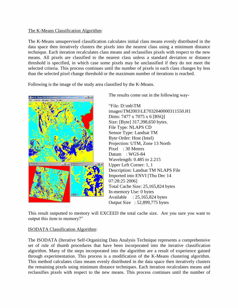
The K-Means Classification Algorithm:

The K-Means unsupervised classification calculates initial class means evenly distributed in the

data space then iteratively clusters the pixels into the nearest class using a minimum distance

technique. Each iteration recalculates class means and reclassifies pixels with respect to the new

means. All pixels are classified to the nearest class unless a standard deviation or distance

threshold is specified, in which case some pixels may be unclassified if they do not meet the

selected criteria. This process continues until the number of pixels in each class changes by less

than the selected pixel change threshold or the maximum number of iterations is reached.

Following is the image of the study area classified by the K-Means.

The results come out in the following way-

“File: D:\mb\TM

images\TM2003\LE7032040000311550.H1

Dims: 7477 x 7075 x 6 [BSQ]

Size: [Byte] 317,398,650 bytes.

File Type: NLAPS CD

Sensor Type: Landsat TM

Byte Order: Host (Intel)

Projection: UTM, Zone 13 North

Pixel : 30 Meters

Datum : WGS-84

Wavelength: 0.485 to 2.215

Upper Left Corner: 1, 1

Description: Landsat TM NLAPS File

Imported into ENVI [Thu Dec 14

07:28:25 2006]

Total Cache Size: 25,165,824 bytes

In-memory Use: 0 bytes

Available : 25,165,824 bytes

Output Size : 52,899,775 bytes

This result outputted to memory will EXCEED the total cache size. Are you sure you want to

output this item to memory?”

ISODATA Classification Algorithm:

The ISODATA (Iterative Self-Organizing Data Analysis Technique represents a comprehensive

set of rule of thumb procedures that have been incorporated into the iterative classification

algorithm. Many of the steps incorporated into the algorithm are a result of experience gained

through experimentation. This process is a modification of the K-Means clustering algorithm.

This method calculates class means evenly distributed in the data space then iteratively clusters

the remaining pixels using minimum distance techniques. Each iteration recalculates means and

reclassifies pixels with respect to the new means. This process continues until the number of

pixels in each class changes by less than the selected pixel change threshold or the maximum

number of iterations is reached.

Following is the image of the study area classified by the ISODATA Technique.

The results come out in the following way-

File: D:\mb\TM images

TM2003\

LE7032040000311550.H1

Dims: 7477 x 7075 x 6 [BSQ]

Size: [Byte] 317,398,650 bytes

File Type: NLAPS CD

Sensor Type: Landsat TM

Byte Order: Host (Intel)


Pixel: 30 Meters

Datum: WGS-84

Wavelength: 0.485 to 2.215

Upper Left Corner: 1, 1

Description: Landsat TM NLAPS File

Imported into ENVI [Thu Dec 14

07:28:25 2006]

Analysis:

The original image-

Location Display ID

Original Image

Screen Data

R G B R G B

28°53'8.03"N,

105°18'13.40"W 59,493,466 122 136 137 86 150 20

28°52'24.91"N,

105°25'35.15"W 55,503,509 114 0 0 84 57 66

28°56'27.64"N,

105°25'36.14"W 55,503,260 61 88 90 70 124 102

28°50'4.54"N,

105°25'34.58"W 55,503,653 95 121 126 79 142 116

28°50'4.76"N,

105°18'12.86"W 59,493,654 80 118 116 75 140 112

28°56'33.71"N,

105°18'15.10"W 59,483,255 26 56 69 61 106 94

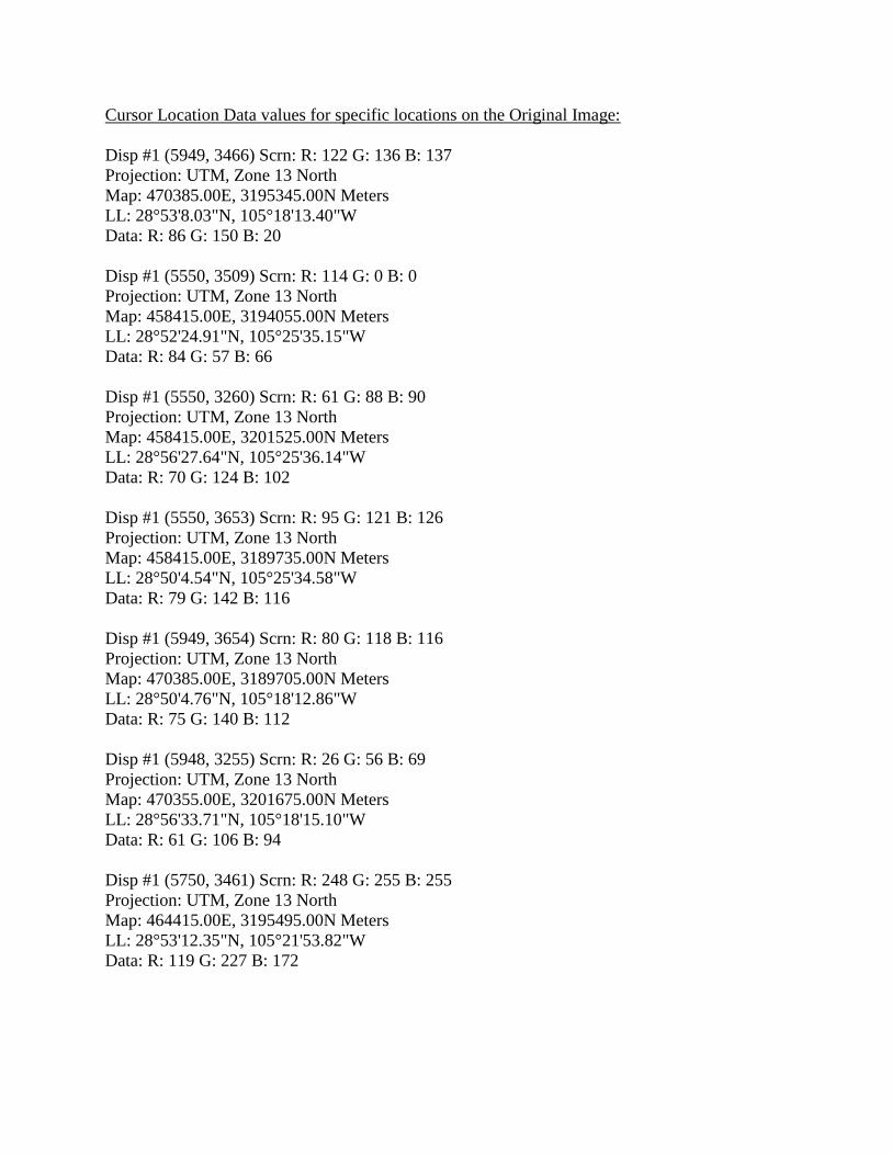
Cursor Location Data values for specific locations on the Original Image:

Disp #1 (5949, 3466) Scrn: R: 122 G: 136 B: 137


Map: 470385.00E, 3195345.00N Meters

LL: 28°53'8.03"N, 105°18'13.40"W

Data: R: 86 G: 150 B: 20

Disp #1 (5550, 3509) Scrn: R: 114 G: 0 B: 0


Map: 458415.00E, 3194055.00N Meters

LL: 28°52'24.91"N, 105°25'35.15"W

Data: R: 84 G: 57 B: 66

Disp #1 (5550, 3260) Scrn: R: 61 G: 88 B: 90


Map: 458415.00E, 3201525.00N Meters

LL: 28°56'27.64"N, 105°25'36.14"W

Data: R: 70 G: 124 B: 102

Disp #1 (5550, 3653) Scrn: R: 95 G: 121 B: 126


Map: 458415.00E, 3189735.00N Meters

LL: 28°50'4.54"N, 105°25'34.58"W

Data: R: 79 G: 142 B: 116

Disp #1 (5949, 3654) Scrn: R: 80 G: 118 B: 116


Map: 470385.00E, 3189705.00N Meters

LL: 28°50'4.76"N, 105°18'12.86"W

Data: R: 75 G: 140 B: 112

Disp #1 (5948, 3255) Scrn: R: 26 G: 56 B: 69


Map: 470355.00E, 3201675.00N Meters

LL: 28°56'33.71"N, 105°18'15.10"W

Data: R: 61 G: 106 B: 94

Disp #1 (5750, 3461) Scrn: R: 248 G: 255 B: 255


Map: 464415.00E, 3195495.00N Meters

LL: 28°53'12.35"N, 105°21'53.82"W

Data: R: 119 G: 227 B: 172

Location Display ID

K-Means

Screen Data

R G B R G B

28°53'8.03"N,

105°18'13.40"W 59,493,466 255 255 0 86 150 120

28°52'24.91"N,

105°25'35.15"W 55,503,509 255 255 0 81 128 105

28°56'27.64"N,

105°25'36.14"W 55,503,260 255 255 0 70 129 107

28°50'4.54"N,

105°25'34.58"W 55,503,653 255 255 0 79 142 116

28°50'4.76"N,

105°18'12.86"W 59,493,654 255 255 0 75 140 112

28°56'33.71"N,

105°18'15.10"W 59,483,255 255 0 0 13 45 63

Cursor Location Data values for specific locations on the Image after K-Means Classification:

Disp #2 (5949, 3466) Scrn: R: 255 G: 255 B: 0


Map: 470385.00E, 3195345.00N Meters

LL: 28°53'8.03"N, 105°18'13.40"W

Disp #1 Data: R: 86 G: 150 B: 120

Disp #2 Data: 4 {Class 4}

Disp #2 (5550, 3505) Scrn: R: 255 G: 255 B: 0


Map: 458415.00E, 3194175.00N Meters

LL: 28°52'28.81"N, 105°25'35.17"W

Disp #1 Data: R: 81 G: 128 B: 105


Disp #2 (5550, 3285) Scrn: R: 255 G: 255 B: 0


Map: 458415.00E, 3200775.00N Meters

LL: 28°56'3.27"N, 105°25'36.04"W

Disp #1 Data: R: 70 G: 129 B: 107


Disp #2 (5550, 3653) Scrn: R: 255 G: 255 B: 0


Map: 458415.00E, 3189735.00N Meters

LL: 28°50'4.54"N, 105°25'34.58"W

Disp #1 Data: R: 79 G: 142 B: 116


Disp #2 (5949, 3654) Scrn: R: 255 G: 255 B: 0


Map: 470385.00E, 3189705.00N Meters

LL: 28°50'4.76"N, 105°18'12.86"W

Disp #1 Data: R: 75 G: 140 B: 112


Disp #2 (5947, 3285) Scrn: R: 255 G: 0 B: 0


Map: 470325.00E, 3200775.00N Meters

LL: 28°56'4.46"N, 105°18'16.13"W

Disp #1 Data: R: 13 G: 45 B: 63


Location Display ID

ISODATA

Screen Data

R G B R G B

28°53'8.03"N,

105°18'13.40"W 59,493,466 0 255 255 - - -

28°52'24.91"N,

105°25'35.15"W 55,503,509 0 0 255 - - -

28°56'27.64"N,

105°25'36.14"W 55,503,260 0 255 255 - - -

28°50'4.54"N,

105°25'34.58"W 55,503,653 255 0 255 - - -

28°50'4.76"N,

105°18'12.86"W 59,493,654 255 0 255 - - -

28°56'33.71"N,

105°18'15.10"W 59,483,255 255 0 0 - - -

Cursor Location Data values for specific locations on the Image after ISODATA Classification:

Disp #2 (5949,3466) Scrn: R:0 G:255 B:255


Map: 470385.00E,3195345.00N Meters

LL : 28°53'8.03"N, 105°18'13.40"W

Data: 5 {Class 5}

Disp #2 (5553,3508) Scrn: R:0 G:0 B:255


Map: 458505.00E,3194085.00N Meters

LL : 28°52'25.90"N, 105°25'31.83"W

Data: 3 {Class 3}

Disp #2 (5550,3286) Scrn: R:0 G:255 B:255


Map: 458415.00E,3200745.00N Meters

LL : 28°56'2.29"N, 105°25'36.04"W

Data: 5 {Class 5}

Disp #2 (5550,3652) Scrn: R:255 G:0 B:255


Map: 458415.00E,3189765.00N Meters

LL : 28°50'5.52"N, 105°25'34.58"W

Data: 6 {Class 6}

Disp #2 (5949,3648) Scrn: R:255 G:0 B:255


Map: 470385.00E,3189885.00N Meters

LL : 28°50'10.61"N, 105°18'12.88"W

Data: 6 {Class 6}

Disp #2 (5949,3289) Scrn: R:255 G:0 B:0


Map: 470385.00E,3200655.00N Meters

LL : 28°56'0.57"N, 105°18'13.90"W

Data: 1 {Class 1}

a remote sensing application for image classification

Documents