remote sensing techniques for forest parameter … · 443 vohland, stoffels, hau and schüler...

441

www.metla.fi/silvafennica · ISSN 0037-5330The Finnish Society of Forest Science · The Finnish Forest Research Institute

Remote Sensing Techniques for Forest Parameter Assessment: Multispectral Classification and Linear Spectral Mixture Analysis

Michael Vohland, Johannes Stoffels, Christina Hau and Gebhard Schüler

Vohland, M., Stoffels, J., Hau, C. & Schüler, G. 2007. Remote sensing techniques for forest parameter assessment: multispectral classification and linear spectral mixture analysis. Silva Fennica 41(3): 441–456.

One of the most common applications of remote sensing in forestry is the production of thematic maps, depicting e.g. tree species or stand age, by means of image classification. Nevertheless, the absolute quantification of stand variables is even more essential for forest inventories. For both issues, satellite data are attractive for their large-area and up-to-date mapping capacities. This study followed two steps, and at first a supervised parametric clas-sification was performed for a German test site based on a radiometrically corrected Landsat-5 TM scene. There, eight forest classes were identified with an overall accuracy of 87.5%. In the following, the study focused on the estimation of one key stand variable, the stem number per hectare (SN), which was carried out for a number of Norway spruce stands that had been clearly identified in the multispectral classification. For the estimation of SN, the approach of Linear Spectral Mixture Analysis (LSMA) was found to be clearly more effective than spectral indices. LSMA is based on the premise that measured reflectances can be linearly modelled from a set of so-called endmember spectra. In this study, the endmember sets were held variable to decompose pixel values to abundances of a vegetation, a background (soil, litter, bark) and a shade fraction. Forest structure determines the visible portions of these fractions, and therefore, a multiple regression using them as predictor variables provided the best SN estimates. LSMA allows a pixel-by-pixel quantification of SN for complete satellite images. This opens the view to exploit these data for an improved calibration of large-scale multi-parameter assessment strategies (e.g. statistical modelling or the kNN method for satellite data interpretation).

Keywords Picea abies, stand variables, stem number, remote sensing, multispectral classifica-tion, Linear Spectral Mixture AnalysisAddresses Vohland, Stoffels, Hau: University of Trier, Faculty of Geography and Geosciences, Remote Sensing Department, Trier, Germany; Schüler: Research Institution for Forest Ecology and Forestry (FAWF), Department of Forest Growth and Silviculture, Trippstadt, GermanyE-mail [email protected] 28 February 2007 Revised 2 July 2007 Accepted 13 July 2007Available at http://www.metla.fi/silvafennica/full/sf41/sf413441.pdf

Silva Fennica 41(3) research articles

442

Silva Fennica 41(3), 2007 research articles

1 Introduction

Management of forest stands needs periodic sur-veys of structural stand parameters. As the tra-ditional inventory strategies (field observations, analysis of aerial photographs) are cost-intensive and time-consuming, multispectral remote sen-sing data seem to be attractive to complement and optimise forest inventories. Based on the sensor specific ground resolution (e.g. Landsat-5 TM with 30 m pixels in the reflective domain) and the scene coverage (scan width of 185 km for Landsat TM), multiscale approaches covering both single stands and complete forest regions are feasible by the integration of satellite data.

In Germany, the forest inventory practice has undergone certain modifications in the last years. For stand age definition, the classical nomen-clature (e.g. pole stage, timber tree) refers to the dominant breast height diameter; this system has been extended by a more multifunctional nomenclature – similar to the definition of forest ecotopes – which is based on certain develop-ment stages (foundation and establishment of seedles – stand qualification – dimensioning (crop tree definition and treatment for target stocking) – maturing). Nonetheless, the classes of both nomenclature systems can be assigned to total stand ages specifically for each tree species.

Thus, providing tree species and age classes is one of the main objectives of a number of remote sensing studies. Franklin (1994), Vohland (1997) or Salajanu and Olson (2001), for example, have used multispectral satellite data for forest clas-sification. To be operational, acceptable accuracy levels should be provided by remote sensing clas-sification approaches to obtain both useful and regularly updated inventory data (see Czaplewski and Patterson 2003 for further discussion). How-ever, accuracy actually depends on the properties of the forest stands (e.g. heterogeneity of tree species and age class composition or the vertical structure) as well as the remote sensor and its spe-cific spectral and spatial resolution. Furthermore, an appropriate radiometric image processing is also crucial to obtain image products of consist-ent quality (Woodcock et al. 2001, Peddle et al. 2003). In practice, radiometric preprocessing strategies vary from completely ignoring effects

of atmosphere and illumination to empirical and eventually physically-based correction methods (see Peddle et al. 2003). For a reliable and consist-ent thematic analysis of one selected Landsat-5 TM dataset, this study realises a model based preprocessing approach for the correction of both atmospheric and topographic distortions. After preprocessing, a portion of the Landsat scene (covering a German test site) is subjected to forest classification for tree species and age class defini-tion; afterwards, results are briefly discussed and an error matrix is prepared.

The stand age has been shown by e.g. Siipilehto (2006) to be a key parameter for the statistical assessment of additional stand parameters (e.g. mean and dominant diameter or height, diameter and height of the basal area-median tree, total basal area, total stem number). In that study, predictions were made for 227 Norway spruce (Picea abies) stands of the Finnish national forest inventory and based on multiple linear regressions using total age and site characteristics (e.g. degree days, stoniness or paludification). Nevertheless, predictions were only moderate (RMSE 34–41%) for the sum variables of basal area and stem number, but increased significantly when calibrat-ing the model with known stand variables; in fact, using only one additional sum and one additional mean variable for model calibration was most effective to obtain high prediction accuracies for all unknown variables. This calls attention to the potentials for efficient variable retrieval from multispectral satellite data to contribute to a precise prediction of all structural stand char-acteristics. For the forest site investigated in this study, we concentrated on stands of Picea abies to go beyond the pure classification approach. We applied the relatively simple physical approach of Linear Spectral Mixture Analysis (LSMA) that tries to decompose the heterogeneous mixing of different components (e.g. soil, vegetation) spectrally for each image pixel. Fractional cover estimates derived from LSMA have proven useful in some studies of temperate and boreal forests to characterise structural canopy variables (e.g. leaf area index or canopy closure, see overview by Asner et al. 2003). In this study, LSMA is applied to retrieve the standwise stem number from the selected Landsat TM data. If known, this variable may be helpful to improve the assessment of other

443

Vohland, Stoffels, Hau and Schüler Remote Sensing Techniques for Forest Parameter Assessment: Multispectral Classification and …

stand parameters and to predict the stand struc-ture (e.g. tree diameter distribution) by means of statistical models (Siipilehto 1999, 2006). In addition, it can be used as stand-alone variable to provide information about backlogs of thinning, and to indicate the structural diversity of forest stands in terms of an ecological assessment.

2 Materials and Methods

2.1 Study Area

The test site Idarwald forest (Lat. 49.85°N, Lon. 7.15°E) is located on the north-western slopes of the Hunsrück low mountain range (Rhineland-Palatinate, Germany) (Fig. 1). Near the ridge, poor sandy and shallow soils developed on Devo-nian quartzite bedrock are typical. On the lower parts of the slopes, the solifluction of loamy weathering products from the Tertiary have led to compacted and partly impermeable strata with stands of Betula pubescens. In the other parts of the study region with permeable soils, the Luzulo-Fagetum typicum and the Luzulo-Fage-tum milietosum were the original natural forest communities; nevertheless, Picea abies became dominant by silviculture since the late 18th cen-

tury. Thus, the proportion of Picea abies in all tree species of the Idarwald region is actually still the highest, although a gradual conversion to mixed forests has begun in the late eighties.

The total area of the Idarwald is about 7500 ha in size. For our analysis, two forestry districts (Hinzerath, Bischofsdhron) with an area of about 1773 ha were selected. In these districts, homo-geneous stands of one species and age class can be found as well as heterogeneous mixed stands with underplanting or natural regeneration.

2.2 Forest Inventory Data and Aerial Photographs

Forest inventory data were integrated in the clas-sification approach as they allow the extraction of training data and also the validation of the classification results. For this purpose, official inventory data were made available by the forest management of Rhineland-Palatinate (end of col-lection period: October 1994). These data were originally included in some hierarchically ordered data files providing information about the forest region, the single forest stands and the respec-tive tree species. After some editing for a stand-wise data aggregation, they were integrated in a digital forest GIS (FIS) and related to the vector

Fig. 1. The study site Idarwald forest (Rhineland Palatinate, Germany).

444


data (stand polygons) digitised from the official forest map. Additionally, color infrared (CIR) aerial photopraphs from an overflight carried out on August 4, 1990 were available through the Research Institution for Forest Ecology and Forestry (FAWF) of Rhineland-Palatinate. The photographs were scanned and orthorectified, and as their scale (1:11 000) allows the separation of single trees, the crowns were counted standwise to validate the LSMA based estimates from Landsat-5 TM data (see 2.3.3).

2.3 Satellite Imagery

2.3.1 Availabe Landsat TM Data and Steps of Preprocessing

In this study, one Landsat-5 TM scene cover-ing the Hunsrück area (Landsat path: 196; row: 25) around the time the CIR data were acquired was selected for analysis (15.07.1990). Landsat-5 TM provides multispectral reflective data in the spectral domains of the visible, the near infrared and the shortwave infrared (Table 1), and there-fore is appropriate for the study of vegetation characteristics.

The data set was calibrated by converting the original digital numbers to absolute reflectance values for each pixel. As the terrain of the study area is very rugged, the removal of topographic effects is important prior to the analysis of the forest structure. The key factor in the topographic correction is the correct pixel-by-pixel estimation of the total illumination (direct and diffuse terms), which is not feasible by typical “stand-alone” cor-rection approaches (Lambertian cosine or Min-naert correction) that do not integrate atmospheric processes (Conese et al. 1993, Hill et al. 1995). Thus, we decided to pursue an integrated approach of a combined atmospheric and topographic cor-rection by means of the software package AtCPro (Atmospheric Correction Processing of Multi- & Hyperspectral Data; Hill et al. 1995). In AtCPro, a

modified version of the 5S-radiative transfer code of Tanré et al. (1990) is implemented to account for both atmospheric scattering and atmospheric absorption by H2O, O3, CO2 and O2. On the basis of this model, terms describing illumination can be approximated and finally compensated for each raster cell by the integration of a digital elevation model (DEM) (Fig. 2). In addition to the radio-metric correction, data preprocessing comprised a precise georectification, which allows a multi-layer analysis combining e.g. Landsat TM image data and vector data of the FIS.

2.3.2 Multispectral Classification Approach

In general, classification approaches aim at the production of a thematic map from multispectral satellite imagery. They are based on the principle that different objects or land cover types show typical reflectance properties which are at best clearly distinguishable in the multispectral feature space. Thus, the actual level of detail of the con-structed thematic map depends on the particular separability of the relevant categories which, in this study, are forest types or forest classes.

Thematic classification involves several steps of data analysis. After an optional preprocessing to convert the original data to absolute reflectance values (data calibration, 2.3.1), training samples representing different forest types are extracted from the image data and tested for separability by signature analysis. For the Idarwald classifi-cation, this selection was based on the FIS data, and only homogeneous stands (i.e. stands made up by more than 90% of one species) were used for the supervised (based on a priori-knowledge) definition of training samples. Thereafter, repre-sentative and also statistically differing samples are used to train the classifier. For multispectral remote sensing data, the maximum likelihood approach is a widely used classification method. In this approach, Gaussian probability distribu-tion is assumed for each class, and the mean

Table 1. Reflective channels of the Landsat-5 TM sensor (Kramer 2002).

Band TM 1 TM 2 TM 3 TM 4 TM 5 TM 7

Band edges [µm] 0.45–0.52 0.52–0.60 0.63–0.69 0.76–0.90 1.55–1.75 2.08–2.35

445


vectors and covariance matrices are calculated from the selected training data to describe the individual class properties. After this, each pixel can be labelled whereas the class assignment depends on the highest probability of membership (Schowengerdt 2006). This standard parametric approach was applied to the TM data of 1990, and a detailed confusion matrix was computed for validation.

2.3.3 Quantitative Analysis by LSMA

In case of forest cover, an image pixel of Landsat TM can be assumed to comprise a mixture of vegetation, soil or litter components, which can be both sunlit or shaded. Thus, pixel analysis should be based on an adequate unmixing approach.

LSMA considers reflectance values of each pixel (R) as an additive mixture of reflectances of pure materials or cover types (endmembers, E); the contribution of each endmember is deter-mined by its abundance (fractional coverage F) according to Eq. 1:

Ri Fj REij Fji

j

n

j

n

= ⋅ + == =

∑ ∑ε and1 1

1 (1)

withRi = reflectance value in spectral band iREij = spectral signature of endmember j in band iFj = abundance of endmember jεi = residual in spectral band in = number of endmembers

Inverting this mixture model, one retrieves the pixelwise abundances of the considered endmem-bers from the measured pixel values. To produce physically realistic results, one constraint was implemented that forces the retrieved fraction abundances to sum to 1.0. Nevertheless, negative values are possible and may indicate the use of endmembers that are not part of the given mixture (Rogge et al. 2006). The root mean squared error (RMSE) is retrieved for each pixel when compar-ing the measured spectra with those reconstructed from the endmembers and their abundances; it represents the spectral information that cannot be explained by the selected mixture model. How-

Fig. 2. The radiometric preprocesssing chain for the Landsat-5 TM data.

446


ever, the number of endmembers to be included in the model is restricted by the intrinsic dimen-sion of the spectral data. For Landsat TM with highly correlated spectral bands, the number of endmembers should not exceed four (Drake and Settle 1989).

Spectral mixtures including green vegetation tend to be nonlinear due to near infrared trans-mission and scattering; the degree of nonlinear-ity varies depending on soil reflectance and leaf transmittance. However, with coniferous forest the degree of nonlinearity is low so that the premise of LSMA (light interacts with only one material) seems to be sufficiently valid (Roberts et al. 1991, Roberts et al. 1993). Another shortcom-ing of traditional LSMA using fixed endmember sets is its failure to account for variability in the endmember reflectance within images (Asner et al. 2003). The latter can partly be overcome by introducing multiple endmember sets.

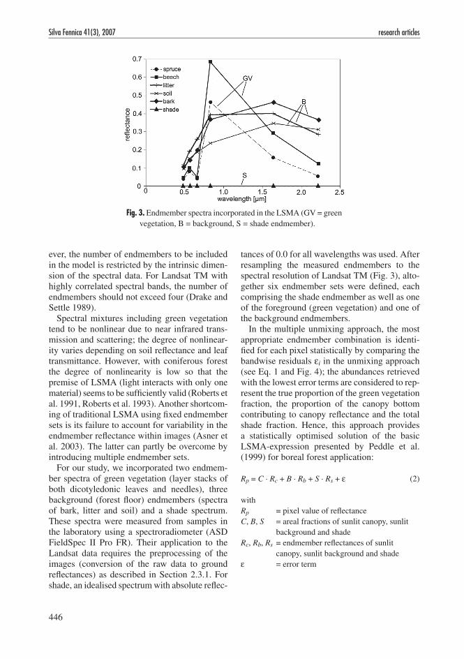
For our study, we incorporated two endmem-ber spectra of green vegetation (layer stacks of both dicotyledonic leaves and needles), three background (forest floor) endmembers (spectra of bark, litter and soil) and a shade spectrum. These spectra were measured from samples in the laboratory using a spectroradiometer (ASD FieldSpec II Pro FR). Their application to the Landsat data requires the preprocessing of the images (conversion of the raw data to ground reflectances) as described in Section 2.3.1. For shade, an idealised spectrum with absolute reflec-

tances of 0.0 for all wavelengths was used. After resampling the measured endmembers to the spectral resolution of Landsat TM (Fig. 3), alto-gether six endmember sets were defined, each comprising the shade endmember as well as one of the foreground (green vegetation) and one of the background endmembers.

In the multiple unmixing approach, the most appropriate endmember combination is identi-fied for each pixel statistically by comparing the bandwise residuals εi in the unmixing approach (see Eq. 1 and Fig. 4); the abundances retrieved with the lowest error terms are considered to rep-resent the true proportion of the green vegetation fraction, the proportion of the canopy bottom contributing to canopy reflectance and the total shade fraction. Hence, this approach provides a statistically optimised solution of the basic LSMA-expression presented by Peddle et al. (1999) for boreal forest application:

Rp = C · Rc + B · Rb + S · Rs + ε (2)

withRp = pixel value of reflectanceC, B, S = areal fractions of sunlit canopy, sunlit

background and shadeRc, Rb, Rs = endmember reflectances of sunlit

canopy, sunlit background and shadeε = error term

Fig. 3. Endmember spectra incorporated in the LSMA (GV = green vegetation, B = background, S = shade endmember).

447


Unlike vegetation indices that are computed from some spectral combination of remote sen-sing data (e.g. by differencing or rationing the measurements in the near infrared and the visible red), the fractional cover estimates of the LSMA are derived by a simple additive model of the radi-ative transfer inside canopies and can therefore be interpreted as physical stand properties. This might allow a close and physically reasonable link to canopy structural properties most relevant for ecological issues or routinely recorded by forest inventory. Local variations can be accounted for by the multiple endmember approach, which is desirable in terms of a generalised application to a wide range of situations (Baret et al. 2000, Asner et al. 2003).

In this study, the unmixing approach was applied to the TM data and afterwards validated by the counts from the aerial photographs. For a detailed analysis and validation, a total of 42 Picea abies stands of the timber tree class with an area of 0.9 to 2.5 hectares were selected from the Idarwald districts. With reference to the FIS data, their absolute age in 1990 varied from 42 to 130 years. For young timber tree stands, canopy closures and stem numbers usually vary greatly due to dif-ferences in management and thinning activities. In the middle and older timber tree stands, stem number keeps constant whereas canopy closures gradually increase. After maturity, felling activi-ties cause the reduction of both canopy closure and stem number. In consequence of this managerial differentiation, and as some of the selected stands were clearly affected by storm damages, the stem

number per hectare varied greatly between 0 and 979 trees per hectare, according to the counts from the aerial photographs. Due to this variation, not only the fraction of green vegetation, but also the sunlit background or the total shade fraction may probably provide efficient diagnostics of the canopy structure.

In this context, some existing studies (Hall et al. 1995, Peddle et al. 1999, Sabol et al. 2002) have demonstrated the power of the shade fraction for assessing biophysical structural information (biomass, leaf area index, net primary productiv-ity, canopy closure). For example, in the study of Sabol et al. (2002) a combination of the LSMA fractions of vegetation and shade proved to be more efficient for identifying increasing crown closure associated with forest regrowth than the classical NDVI (Normalized Difference Vegeta-tion Index; Rouse et al. 1974, see Eq. 3). Never-theless, the stem number – selected in this study as structural forest attribute – is more typically recorded in forest management systems than the crown closure. In the following, the power of the LSMA as predictor for the stem number of the selected Picea abies stands is investigated and also compared to the concept of spectral vegeta-tion indices.

NDVIR R

R R

nIR red

nIR red=

−+

(3)

withRnIR = reflectance in the near infaredRred = reflectance in the visible red

Fig. 4. LSMA approach with multiple endmember sets.

448


3 Results

In the spectral signature analysis some of the training classes turned out to be not separable due to their spectral similarity; thus, altogether eight forest classes potentially separable were defined by training samples (Table 2) and afterwards used for assigning all forest pixels in the classification process for the TM data (Fig. 5).

To assess the accuracy of the classification results, we selected possible reference points (pixels) randomly in the area of the classified forest districts. From this sample, those points were finally chosen which could be assigned to one stand unambiguously (no mixed pixels at stand borders), which allowed a clear stand characterisation from the available FIS data, and

which had not been used as training data. For the latter, the quantity of data was sufficient for five of the eight classes to avoid an overlap between training and validation data (669 reference points); however, for three forest classes (deciduous forest both pole and timber stage, pole stage of doug-las fir and larch) no independent validation data could be extracted, and a total of 220 points that had been used in the training were now applied for validation (Table 3). In the following, the extracted validation points were compared to the multispectral classification results in terms of a confusion matrix (Table 3), which is the standard error matrix for reporting the accuracy of remote sensing classification results (Congalton 1991, Foody 2002). For the Idarwald classification, the overall accuracy was 87.5% (778 from 889 pixels were classified correctly), and the accu-

Table 2. Forest classes as defined by FIS selection and signature analysis from Landsat TM data (15.07.1990).

Age class Development stage Species

Clearcuts, windfalls – –Seedles Establishment Fagus sylvatica, Quercus robur, Quercus petraea, Alnus glutinosa, Picea abiesThickets Stand qualification Picea abies, Pseudotsuga menziesii, Abies alba1

Pole stage Dimensioning Picea abiesPole stage Dimensioning Pseudotsuga menziesii, Larix decidua, Larix kaempferiPole stage Dimensioning Fagus sylvatica, Quercus robur, Quercus petraea, partly mixed with Betula pendula, Alnus glutinosaTimber and matured Maturing Fagus sylvatica, Quercus robur, Quercus petraea, timber stage Betula pubescensTimber and matured Maturing Picea abies2

timber stage

1 no occurrence of homogeneous thickets of deciduous species2 no occurrence of timber tree stands of other coniferous species

Table 3. Confusion matrix of the TM data classification resulting from randomly sampled pixels.

Reference data from FIS A B C D E F G H J

A Clearcuts, windfalls 6 1 1 0 0 0 0 0 8B Seedles 2 9 5 1 0 0 0 0 17C Thickets 0 1 167 8 4 8 4 3 195D Norway Spruce pole stage 2 0 7 90 4 9 0 0 112E Douglas Fir, Larch pole stage1 0 0 0 3 34 4 0 0 41F Norway Spruce timber stage 0 2 4 11 7 313 0 0 337G Deciduous Forest pole stage1 0 4 7 0 0 0 133 2 146H Deciduous Forest timber stage1 0 0 0 0 0 0 7 26 33

J Sum 10 17 191 113 49 334 144 31 889

1 reference points were also used as training data

Dat

a fr

om m

ulti

spec

tral

clas

sific

atio

n

449


racies retrieved for the individual classes were generally in excess of 75%. Solely the class of seedles showed poorer results, but significance is limited here and also for the class of clearcuts and windfalls due to a very small number of reference points.

Another widespread estimate of accuracy is provided by Cohen’s kappa coefficient (κ) (Cohen 1960, Hudson and Ramm 1987), an omnibus index comparing the actual agreement of categori-

cal data against that which might be expected by chance. In reality, the kappa coefficient, that is computed from the confusion matrix as shown in Eq. 4, usually ranges between 0 (no agreement above that expected by chance) and 1 (perfect agreement) (Lillesand and Kiefer 2003). For the Idarwald classification, a relatively high kappa coefficient of 0.836 was calculated which again suggests reliable classification results. Neverthe-less, the analytical value of the kappa coefficient

Fig. 5. Distribution of the forest classes for the Idarwald districts (1990).

450


may be questionable as discussed in detail by Stehmann (1997).

κ =−

−

×

×

==

=

∑∑

∑

n x x x

n x x

ii i i

i

r

i

r

i i

i

r

( )

( )

. .

. .

11

1

(4)

withr = number of rows in the error matrixxii = the number of observations in row i and

column i (major diagonal)xi. = total of observations in row ix.i = total of observations in column in = total number of observations (pixels)

In the classification map (Fig. 5), the high rate of clearings (4.8% of the classified area) is striking. This is due to extreme damages in early spring 1990 by severe windstorms (Vivian and Wiebke) which primarily attacked stands of the shallow root Picea abies. Nevertheless, Picea abies is the most widespread tree species in 1990, and its pole and timber tree stands amount to 42.5% of the classified area.

All pixels of the TM data that had been clas-sified multispectrally were also subjected to the linear spectral unmixing, and the total six pre-defined spectral endmember sets were allowed for unmixing. Finally, 45.3% of all pixels were unmixed with the spectrum of green spruce nee-dles, whereas in 54.7% of all cases the beech leaves endmember provided better model fits. In terms of the background endmember, the bark spectrum was used for the clear majority of pixels (66.4%, soil spectrum: 18.8%, litter spectrum: 14.8%). In view of the forest classes, unmixing

results were consistent (Table 4). For nearly all pixels falling into the class of deciduous forest (> 99%), the spectrum of beech leaves was identi-fied as the most appropriate, and the vast majority of the spruce stands were unmixed with the spruce needle spectrum as foreground endmember. For all classified pixels, a small RMSE in terms of absolute reflectance was obtained (0.0074), which reveals a nearly accurate reconstruction of the pixel spectra by the multiple mixing models.

For each of the 42 selected stands, a spec-tral sensitivity analysis was performed; spectral indices were calculated from the spectral stand signatures and the pixel-based unmixing results were aggregated for each stand.

The sensitivity analysis (Fig. 6) reveals clear changes in the spectra connected with an increas-ing number of stems per hectare. Evidently, the signatures are highly variable in the channels TM 3 (visible red), TM 4 (nIR) and TM 5 and TM 7 (shortwave infrared/swIR). Nevertheless, the prediction power of one channel-reflectances is limited by saturation tendencies for canopies exceeding a number of 400 stems per hectare and by ambiguities (e.g. the reflectances in the nIR can be high for both windfalls with low stem numbers and also dense canopies). The latter is partly compensated by the normalised difference concept used for the NDVI. However, the spec-tral sensitivity analysis showed the swIR to be promising for predicition; thus, another normal-ised difference index known as broadband NDWI (Normalised Difference Water Index (Gao 1996, Jackson et al. 2004), see Eq. 5) was applied.

Table 4. Results of the multiple LSMA for the classified forest pixels (foreground and background endmembers as used for unmixing (in %); mean RMSE (in absolute reflectance) of mixture analysis).

Foreground (leaves) Background RMSE spruce beech barch soil litter

Clearcuts, windfalls 40.1 59.9 94.9 3.1 2.0 0.013Seedles 24.1 75.9 97.1 2.4 0.5 0.015Thickets 31.8 68.2 68.1 22.7 9.2 0.008Douglas fir (pole stage) 67.3 32.7 50.7 37.5 11.8 0.005Norway spruce (pole stage) 70.2 29.8 64.5 14.2 21.3 0.005Norway spruce (timber stage) 87.1 12.9 47.5 15.5 37.0 0.004Deciduous forest (pole stage) 0.3 99.7 40.5 56.4 3.1 0.011Deciduous forest (timber stage) 0.6 99.4 78.1 18.8 3.1 0.009

451


NDWIR R

R R

nIR swIR

nIR swIR=

−+

(5)

Although NDVI and NDWI are highly correlated (r = 0.97), saturation tendency is less distinct for the NDWI which leads to more accurate estimates of the stem number (Table 5, Fig. 7).

In terms of spectral unmixing, the results for each endmember fraction were plotted against SN to get an idea of the individual response to SN variation (Fig. 8). Obviously, the green vegeta-tion (GV) abundances form the most appropriate stand-alone SN predictor. Quite different from the vegetation indices, the GV fraction is linearly

Fig. 6. Sensitivity analysis: Stands of Picea abies (timber tree class) with different stem numbers per hectare (SN).

Fig. 7. Spectral indices: NDVI vs. NDWI (left) and NDWI-based estimates of SN (right).

Table 5. Statistics for estimates of stem number per hectare by vegetation indices (n = 42).

Index Estimation model r² a RMSE r²cv a,b RMSEcv

b

Rred SN = –390.17 × ln(Rred) – 978.6 0.55 172.8 0.52 179.3RnIR SN = 4387 × RnIR – 290.96 0.13 240.5 0.04 258.4RswIR SN = –459.85 × ln(RswIR) – 682.3 0.58 166.6 0.55 173.3NDVI SN = exp(8.5456 × NDVI – 0.3268) 0.67 168.2 0.65 175.3NDWI SN = exp(5.6225 × NDWI + 4.006) 0.76 152.1 0.74 158.1

a all correlations statistically significant with α < 0.05b results after internal validation performing a leave-one-out crossvalidation (cv)

452


related to SN and not affected by saturation. Thus, by (SN = 2612.5 × FGV – 100.6) one retrieves quite accurate estimates with a low RMSE term (r2

cv = 0.76, RMSEcv = 126, Fig. 9), which is a clear improvement compared to the results of the best-predicting index NDWI (RMSEcv = 158).

Evidently, the quantified endmember abun-dances are strongly related to each other, which plausibly follows from the constrained sum-to-one unmixing approach. The question is whether a significant multiple (linear) regression model can be identified to explain any more variation of SN, beyond the variation explained by the simple GV regression model. Compared to GV, the contribution of the background fraction is opposite in trend; it consistently diminishes with increasing SN, and becomes insensitive for all plots with SN > 400. The interrelation between FB and SN can simply be linearized by taking the logarithm of FB.

The quantified shade fraction abundances clearly reveal the overall high contribution of shade to the spruce canopy reflectances. They steadily increase with SN reaching the maxi-mum within values of 300 to 400 stems per hectare. Here, still moderate densities induce a rough texture and the shadows dropped by the approximately conic crowns are largely visible for the nadir viewing remote sensor. Nevertheless, further SN increase reduces roughness, and the shaded fractions decrease, while the visible sunlit crown fraction grows proportionally to SN.

From the scatterplot it follows that the shade fraction abundances cannot provide satisfactory SN estimates when used solely due to the non-uniqueness of the FS–SN relation. Nevertheless, this does not exclude a gain in estimation power by FS in a multiple analysis. The most appropriate linearizable model to partly represent the interre-lation between the shade fraction abundances and SN is formed by a second order polynomial regres-sion (SN = –10 551 × FS

2 + 12 294 × FS – 2989.7). Based on that, a stepwise linear multiple regres-sion with SN as dependent and FGV, ln(FB), FS

2 and FS as predictor variables was established. In this approach, FGV was selected as first vari-able as it provides the most significant univariate regression. After this, all other variables were selected successively (the second was FS

2, then ln(FB) and FS), as they all turned out to explain residual variation of SN significantly (Table 6, all partial correlation coefficients with α < 0.05). In this process, the coefficient of determination (r²) gradually increased from 0.78 to 0.85, and r²cv also increased from 0.76 to 0.82 (Fig. 9). Compared to the simple regression with FGV, the multiple approach yields a notedly lower RMSEcv (110 instead of 126). Results particularly improve for stands with 600 to 900 stems per hectare with a now clearly reduced scattering around the 1:1-line in the plot of measured versus estimated values (Fig. 9).

Fig. 8. Fractions of green vegetation (GV), background (B) and shade (S) as function of SN (n = 42).

453


4 Discussion and Conclusions

Many papers have dealt with the question of accu-racy assessment strategies for land cover clas-sification from remote sensing data (e.g. Trodd 1995, Thomlinson et al. 1999, Foody 2002). As one outcome, an overall accuracy (percentage of cases correctly classified) of 85% with no class less than 70% has been claimed (Thomlinson et al. 1999). Referring to that, the accuracies obtained for the multispectral classification of the 1990 data are more than adequate, and they agree with or are superior to results achieved by other multispectral forest classifications (Franklin 1994, Vohland 1997, Salajanu and Olson 2001, Schlerf 2006) Nevertheless, the actually reach-able accuracies depend on the complexity of the classification issues and thus seem to be restricted in terms of a direct comparison. In our study, the integration of a broad deciduous forest timber stage-class and a high proportion of spectrally well-defined Norway spruce stands (timber stage)

have certainly contributed to an overall high clas-sification accuracy.

Classification results may be linked to an appro-priate radiometric image preprocessing. This issue was not examined explicitly in this study, but it seems to be highly recommendable to pay close attention to the radiometric consistency of remote sensing data and image products, as the users interested in forest applications will rely on standardised (certified) high-quality data (Peddle et al. 2003).

Furthermore, an adequate preprocessing is mandatory for quantitative approaches combining spectroradiometer and image data. Here, labora-tory measured endmember spectra were integrated for the LSMA approach with multiple endmember sets. By unmixing the pixels of Norway spruce stands, the provided fractions of green vegetation were more powerful for stem number estimation than classical spectral vegetation indices, and the RMSE of prediction clearly improved. For the indices, the NDWI was superior to the NDVI, and

Fig. 9. Estimates of SN based on simple and multiple linear regression using endmember fractions.

Table 6. Coefficients of the final linear multiple regression model for predicting SN.

Constant FGV FS2 ln(FB) FS

Coefficient –883.9 1278.3 –3582.8 –127.2 3507.9Partial correlation – 0.36 –0.38 –0.38 0.33Significance (α) – 0.024 0.017 0.017 0.041

454


it continued to reflect changes of SN by increasing moderately, whereas the NDVI already saturated. This coincides with the findings of Jackson et al. (2004) who tested both indices for retrieving the total vegetation water content that is intrinsically tied to the mass of green vegetation.

The GV fractions provided by LSMA did not saturate and provided reliable SN estimates. Nevertheless, the prediction power again was enlarged significantly by integrating the shade and background fractions in a multivariate regression analysis. This again proves the LSMA to provide a realistic mapping of both sunlit and shaded frac-tions, which is diagnostic for the forest structure and also depends on the actual sun-sensor geo-metry. To normalise the effects of variable solar zenith angels during the Landsat overflight, the vegetation fraction is commonly divided by (1 – shade) to obtain an estimate for the vegetation ground cover (Adams et al. 1995, Asner et al. 2003). Nonetheless, valuable structural informa-tion is eliminated by this normalisation, and for the SN variable studied here, normalised vegeta-tion abundances tended to saturate for high SN values and lost much of their predictive power (in fact, the r2

cv dropped to 0.51 and the RMSEcv clearly increased to 181).

For an operational use, the LSMA approach described in this study may be applied to forest strata identified within multispectral and large area mapping satellite images (of ideally medium to high spatial resolution; e.g. Landsat TM, ASTER, IRS, SPOT). After a careful calibra-tion with some representative reference plots, the prediction model may be used on a pixel-by-pixel basis to provide continuous fields of SN estimates. These data will possibly assist statistical models for forest parameter retrieval or be integrated as a reference for multi-source forest invento-ries based on the k-Nearest Neighbour algorithm (kNN). This aproach, originally developed for the Finnish national forest survey by Tomppo (1990, 1991), is a non parametric classification strategy based on reference pixels with known ground truth forest data. For each pixel with unknown parameter values, k spectrally nearest neighbours are selected and used for forest parameter retrieval by a respective weighting of their terrestrial refer-ence data. Thus, the spectral information is used to carry forest data from reference points to the

whole of forest plots (Holmström et al. 2002).Nevertheless, the accuracy of this approach

simply depends on having enough up-to-date reference data or ground samples “to cover all variations in tree size and stand density for each cover type” (Franco-Lopez et al. 2001).

One way to retrieve reference data is to update the aged information of past inventories by the application of forest growth models, which is limited to the reconstruction of a regular tree and stand development; disturbed plots (due to thinnings, windfalls or calamities) have to be excluded as no input data are available for the growth modelling (Holmström et al. 2002). As alternative, the described pixel-by-pixel approach applied to currently available and full area map-ping satellite data may contribute to close the gap of up-to-date reference data by providing spatially distributed SN estimates.

Acknowledgements

This study was partly funded by the Research Institution for Forest Ecology and Forestry (FAWF) in Rhineland-Palatinate (Germany). The authors like to thank Friedrich Engels (FAWF), Franz Ronellenfitsch and Patrick Lienin for their contribution in the analysis of the aerial photo-graphs. Many thanks to Gerd Womelsdorf, the head of the forestry office Idarwald (formerly head of the forestry office Morbach), for his substantial support concerning field trips and field surveys. We thank Joachim Hill (Remote Sensing Department, University of Trier) for providing helpful software tools.

References

Adams, J.B., Sabol, D.E., Kapos, V., Almeida, R., Rob-erts, D.A., Smith, M.O. & Gillespie, A.R. 1995. Classification of multispectral images based on fractions of endmembers – Application to land-cover change in the Brazilian Amazon. Remote Sensing of Environment 52: 137–154.

Asner, G.P., Hicke, J.A. & Lobell, D.B. 2003. Per-pixel analysis of forest structure. In: Wulder, M.A. &

455


Franklin, S.E. (eds.). Remote sensing of forest environments – Concepts and case studies. Kluwer Academic Publishers. p. 209–254.

Baret, F., Weiss, M., Troufleau, D., Prévot, L. & Combal, B. 2000. Maximum information exploita-tion for canopy characterisation by remote sensing. Aspects of Applied Biology 60: 71–82.

Cohen, J. 1960. A coefficient of agreement for nominal scales. Educational and Psychological Measure-ment 20: 37–64.

Conese, C., Gilabert, M.A., Maselli, F. & Bottai, L. 1993. Topographic normalization of TM scenes through the use of an atmospheric correction method and digital terrain models. Photogram-metric Engineering and Remote Sensing 59: 1745–1753.

Congalton, R.G. 1991. A review of assessing the accu-racy of classifications of remotely sensed data. Remote Sensing of Environment 37: 35–46.

Czaplewski, R.L. & Patterson, P.L. 2003. Classification accuracy for stratification with remotely sensed data. Forest Science 49: 402–408.

Drake, N.A. & Settle, J.J. 1989. Linear mixture mod-elling of Thematic Mapper data of the Peruvian Andes. In: Proc. 9th EARSeL Symp., Helsinki, Finland, 27 June–1 July 1989. p. 490–495.

Foody, G.M. 2002. Status of land cover classification accuracy assessment. Remote Sensing of Environ-ment 80: 185–201.

Franco-Lopez, H., Ek, A.R. & Bauer, M.E. 2001. Estimation and mapping of forest stand density, volume and cover type using the k-nearest neigh-bors method. Remote Sensing of Environment 77: 251–274.

Franklin, S.E. 1994. Discrimination of subalpine forest species and canopy density using digital CASI, SPOT PLA, and Landsat TM data. Photo-grammetric Engineering and Remote Sensing 60: 1233–1241.

Gao, B.C. 1996. A normalized difference water index for remote sensing of vegetation liquid water from space. Remote Sensing of Environment 58: 257–266.

Hall, F.G., Shimabukuro, Y.E. & Huemmrich, K.F. 1995. Remote sensing of forest biophysical struc-ture using mixture decomposition and geometric reflectance models. Ecological Applications 5: 993–1013.

Hay, J.E. & McKay, D.C. 1985. Estimating solar irradi-ance on inclined surfaces: a review and assessment

of methodologies. International Journal of Solar Energy 3: 203–240.

Hill, J., Mehl, W. & Radeloff, V. 1995. Improved forest mapping by combining corrections of atmospheric and topographic effects in Landsat TM imagery. In: Askne, J. (ed.). Sensors and environmental applications of remote sensing. Proc. 14th EARSeL Symp., Göteborg 6–8 June. p. 143–151.

Holmström, H., Nilsson, M. & Ståhl, G. 2002. Fore-casted reference sample plot data in estimation of stem volume using satellite spectral data and the kNN method. International Journal of Remote Sensing 23: 1757–1774.

Hudson, W.D. & Ramm, C.W. 1987. Correct formula-tion of the kappa coefficient of agreement. Pho-togrammetric Engineering and Remote Sensing 53: 421–422.

Jackson, T.J., Chen, D., Cosh, M., Li, F., Anderson, M., Walthall, C., Doriaswamy, P. & Hunt, E.R. 2004. Vegetation water content mapping using Landsat data derived normalized difference water index for corn and soybeans. Remote Sensing of Environ-ment 92: 475–482.

Kramer, H.J. 2002. Observation of the earth and its environment – survey of missions and sensors. Springer. 1510 p.

Lillesand, T.M. & Kiefer, R.W. 2003. Remote sen-sing and image interpretation. John Wiley & Sons. 736 p.

Peddle, D.R., Hall, F.G. & Le Drew, E.F. 1999. Spectral mixture analysis and geometric-optical reflectance modeling of boreal forest biophysical structure. Remote Sensing of Environment 67: 288–297.

— , Teillet, P.M. & Wulder, M.A. 2003. Radiometric image processing. In: Wulder, M.A. & Franklin, S.E. (eds.). Remote sensing of forest environments – concepts and case studies. Kluwer Academic Publishers. p. 181–208.

Roberts, D.A., Smith, M.O., Adams, J.B. & Gillespie, A.R. 1991. Leaf spectral types, residuals and canopy shade in an AVIRIS image. In: Green, R.O. (ed.). Proc. 3rd airborne visible / infrared imaging spectrometer (AVIRIS) workshop, Pasadena, CA, 20–21 May. p. 43–50.

— , Smith, M.O. & Adams, J.B. 1993. Green vege-tation, nonphotosynthetic vegetation and soils in AVIRIS data. Remote Sensing of Environment 44: 255–269.

Rogge, D.M., Rivard, B., Zhang, J. & Feng, J. 2006. Iterative spectral unmixing for optimizing per-pixel

456


endmember sets. IEEE Transactions on Geoscience and Remote Sensing 44: 3725–3736.

Rouse, J.W., Haas, R.H., Schell, J.A., Deering, D.W. & Harlan, J.C. 1974. Monitoring the vernal advance-ment of retrogradation of natural vegetation. NASA/GFC, Type III, Final Report, Greenbelt, MD.

Sabol Jr., D.E., Gillespie, A.R., Adams, J.B., Smith, M.O. & Tucker, C.J. 2002. Structural stage in Pacific Northwest forests estimated using simple mixing models of multispectral images. Remote Sensing of Environment 80: 1–16.

Salajanu, D. & Olson, C.E. 2001. The significance of spatial resolution – Identifying forest cover from satellite data. Journal of Forestry 99: 32–38.

Schlerf, M. 2006. Determination of structural and chemical forest attributes using hyperspectral remote sensing data – Case studies in Norway spruce forests. PhD Thesis, University of Trier. Available at http://ubt.opus.hbz-nrw.de/volltexte/ 2006/369/.

Schowengerdt, R.A. 2006. Remote sensing – models and methods for image processing. Academic Press, Burlington, San Diego, London. 515 p.

Siipilehto, J. 1999. Improving the accuracy of predicted basal-area diameter distribution in advanced stands by determining stem number. Silva Fennica 33: 281–301.

— 2006. Linear prediction application for modelling the relationships between a large number of stand characteristics of Norway spruce stands. Silva Fen-nica 40: 517–530.

Stehmann, S.V. 1997. Selecting and interpreting meas-ures of thematic classification accuracy. Remote Sensing of Environment 62: 77–89.

Tanré, D., Deroo, C., Duhaut, P., Herman, M., Mocrette, J.J., Perbos, J. & Deschamps, P.Y. 1990. Descrip-tion of a computer code to simulate the satellite signal in the solar spectrum – the 5S code. Interna-tional Journal of Remote Sensing 11: 659–668.

Thomlinson, J.R., Bolstad, P.V. & Cohen, W.B. 1999. Coordinating methodologies for scaling landcover classifications from site-specific to global: steps toward validating global map products. Remote Sensing of Environment 70: 16–28.

Tomppo, E. 1990. Designing a satellite image-aided national forest survey in Finland. In: The usability of remote sensing for forest inventory and plan-ning. SNS/IUFRO Workshop, 26–28 February 1990, Report 4. p. 43–47.

— 1991. Satellite imagery-based national inventory of Finland. International Archives of Photogrammetry and Remote Sensing 28: 419–424.

Trodd, N.M. 1995. Uncertainty in land cover mapping for modelling land cover change. In: Remote Sen-sing Society (ed.). Proc. of RSS95 remote sensing in action. p. 1138–1145.

Vohland, M. 1997. Einsatz von Satellitenbilddaten (Landsat TM) zur Ableitung forstlicher Bestands-parameter und Waldschadensindikatoren. Diploma thesis, University of Trier, unpublished. 156 p. (In German).

Woodcock, C.E., Macomber, S.A., Pax-Lenney, M. & Cohen, W.B. 2001. Monitoring large areas for forest change using Landsat: generalization across space, time and Landsat sensors. Remote Sensing of Environment 78: 194–203.

Total of 40 references

remote sensing techniques for forest parameter … · 443 vohland, stoffels, hau and schüler...

Documents