1

A Review of the Basics

2

Learning Objectives

1. Understand the concept of the National Income Identities

2. Understand the definition of Unemployment3. Understand the definition of a price index4. Understand the concept of Economic

equilibrium and how it is influenced by expectations

3

1. NIE Identities

• Review GDP defn in Mankiw 2.1• Before we get into models of economic

behaviour we need to look some definitions and some issues in measurement

• Measurement economic quantities may seem boring…– But it can give crucial insight even without a

model of behaviour– Example: the current crisis

4

NIE Identity

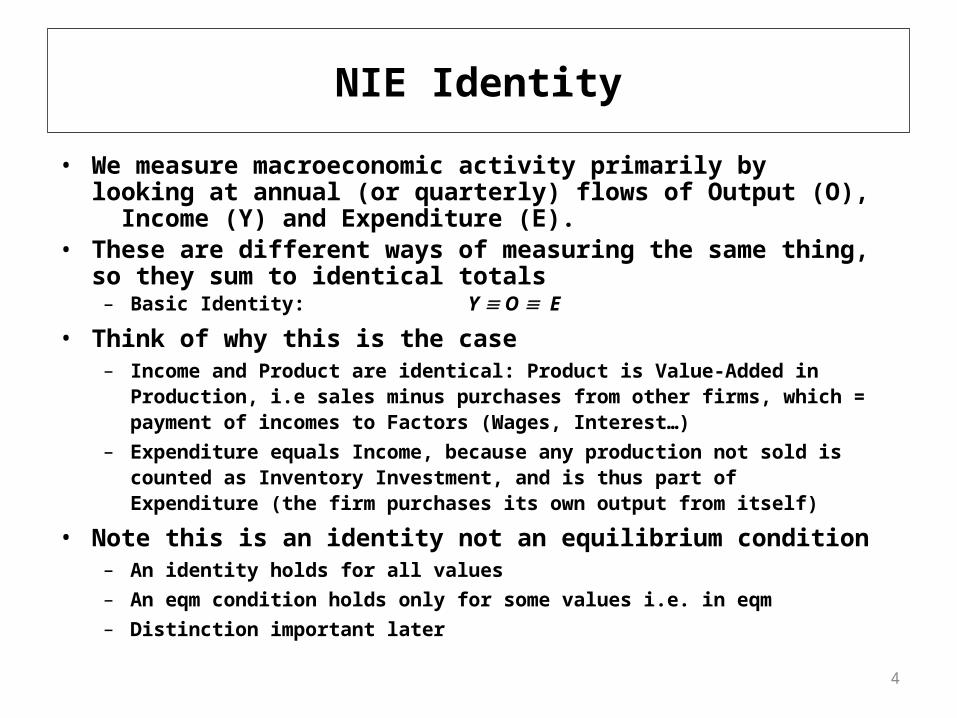
• We measure macroeconomic activity primarily by looking at annual (or quarterly) flows of Output (O), Income (Y) and Expenditure (E).

• These are different ways of measuring the same thing, so they sum to identical totals– Basic Identity: Y O E

• Think of why this is the case– Income and Product are identical: Product is Value-Added in Production, i.e sales

minus purchases from other firms, which = payment of incomes to Factors (Wages, Interest…)

– Expenditure equals Income, because any production not sold is counted as Inventory Investment, and is thus part of Expenditure (the firm purchases its own output from itself)

• Note this is an identity not an equilibrium condition– An identity holds for all values– An eqm condition holds only for some values i.e. in eqm– Distinction important later

5

NIE: GDP vs GNP

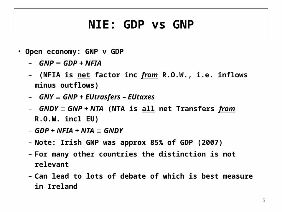
• Open economy: GNP v GDP

– GNP GDP + NFIA

– (NFIA is net factor inc from R.O.W., i.e. inflows minus outflows)

– GNY GNP + EUtrasfers – EUtaxes

– GNDY GNP + NTA (NTA is all net Transfers from R.O.W. incl EU)

– GDP + NFIA + NTA GNDY

– Note: Irish GNP was approx 85% of GDP (2007)

– For many other countries the distinction is not relevant

– Can lead to lots of debate of which is best measure in Ireland

6

NIE: SAVINGS & INVESTMENT IDENTITY

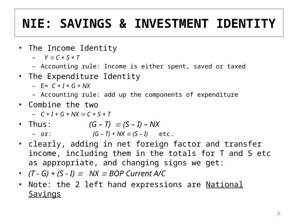
• The Income Identity– Y C + S + T– Accounting rule: Income is either spent, saved or taxed

• The Expenditure Identity– E= C + I + G + NX– Accounting rule: add up the components of expenditure

• Combine the two– C + I + G + NX C + S + T

• Thus: (G – T) (S – I) – NX– or: (G – T) + NX (S – I) etc.

• clearly, adding in net foreign factor and transfer income, including them in the totals for T and S etc as appropriate, and changing signs we get:

• (T - G) + (S - I) NX BOP Current A/C • Note: the 2 left hand expressions are National Savings

7

NIE: SAVINGS & INVESTMENT IDENTITY

• This is often known as the twin deficits identity• Even though it doesn’t involve any model or description of economic

behaviour it can be informative• Implication: a current account surplus can only occur if there is an excess

of national savings• Application 1: The US

– The US has trade deficit (esp with China)– This is inescapable given it has insufficient savings– China surplus equates to surplus Chinese savings

• Application 2: Ireland’s Bubble– We had a bubble (high investment)– Insufficient savings– So high current account deficit

8

Savings

-10.00%

-5.00%

0.00%

5.00%

10.00%

15.00%

20.00%

25.00%

30.00%

35.00%

1995 1996 1997 1998 1999 2000 2001 2002 2003 2004 2005 2006 2007

Personal

Corporate

Gov

Inv

CA

9

• See Mankiw 2.3• The labour force (L) = employed (E) + unemployed (U)• The unemployment rate u% = U/L or U/(E + U)• Letting the population of Labour-force Age = P, we also have:• The Labour force participation rate: LFPR% = L/P• Measuring Employment and Unemployment

– Surveys: household QNHS in Ireland, quarterly household survey (CPS in USA); business surveys for employment.

– Administrative: “Live Register” (Ireland); related to benefit claimants

2. Unemployment

10

Unemployment

• The precise details of how surveys and other measures are constructed will differ from country to country. Survey methods are generally more comparable.

• Key Issue: have to “want” to work to be unemployed as distinct from not working

• Surveys try to capture this: “active search”– Issue of how active– Discouraged worker effects

• There is a difference between what economists’ defn of U and rest of society

• Claimant counts do not – may include people NILF

11

• Mankiw 2.2• Some components of GDP have well-known measures of

inflation: the CPI for household consumption• For a more comprehensive measure the implicit price deflator

for GDP is used: this relates to all items in the GDP• A price index is a weighted average measure of price changes• Two questions arise: (i) what is included (ii) what kind of

weighting system to use– For Consumption the Irish CPI includes a measure of housing costs, the

Eurozone HIPC does not (why?)

• Generally if an index uses base-year weights (Laspeyre), the resulting inflation is higher than if current year weights are used (Paasche)– CPI is Laspeyre

3. Prices

12

• A Laspeyre index of prices uses the quantities prevailing in some base (e.g. survey) year to weight prices. The index takes the form:

• (p1q0 / p0q0)x100

• Note: base-year quantities (q0) are used to compare prices in the two years (p1 and p0 )

• A Paasche index of prices uses the quantities prevailing in the terminal year to weight prices. The index takes the form:

• (p1q1/ p0q1)x100

• Note: current-year quantities (q1) are used to compare prices in the two years (p1 and p0)

• As relatively cheaper are substituted for dearer goods, the Laspeyre index of prices has an upward substitution bias.

• So CPI inflation is biased upwards

Laspeyre vs Pasche

13

4. Equilibrium• Key concept in economics

– illustrate with the simplest possible macro model– Mankiw 11

• Equilibrium is a point of balance or stability– Specifically in economics it is a point where economic agents’ plans are

mutually consistent and therefore are realised• Disequilibrium

– plans are inconsistent – then someone’s plans are not realised– Somebody is disappointed– Behaviour will change– The economy will change– so not stable or balanced

14

MACROECONOMIC EQUILIBRIUM

• First, Output (which equals Income) is a function of inputs: for simplicity, Capital (K) and Labour (L)

Y = f(K, L)– This is the amount firms plan to spend

• There will also be Aggregate Demand or Planned Expenditure (PE)– the amount of Expenditure which agents plan to make – Agents: Households, firms, the Government and foreigners

• In equilibrium plans are consistent Y = PE

• Later we will see that sometimes Output or Income do not equal planned expenditure: this corresponds to a disequilibrium

• The general idea is that in equilibrium the forces acting on some variable (Y) are balanced and hence Y will not change.

15

• Conventionally we look at separate components of aggregate (planned) expenditure: C, I, G, NX. This is because they behave differently.

• Crucially C (Consumption) depends partly on Income: so part of Expenditure depends on Income: hence the term Induced (Consumption) Expenditure

• Other components of Expenditure are Autonomous: this should be understood as depending on something other than Income.

• We have– an Autonomous component of Consumption (Ca)– Investment (I)– Government purchases (G) – Foreign demand (NX)

Planned Expenditure

16

• An equation that describes consumption plans• Very Generally, Consumption depends on Disposable Income (Y minus net

taxes, T). • More specifically: C = Ca + c(Y – T)

– the “Autonomous” and “Induced” elements are on the right-hand side.– For simplicity Mankiw leaves out Ca

• The coefficient c (The Marginal Propensity to Consume) is > 0 and < 1, implying that for any given increase or decrease in disposable income C will change in the same direction, but by a lesser amount.

• i.e. 0 < dC/d(Y – T) = c < 1• This is a model of consumption insofar as it is a simplified representation

of how people make their consumption plans– It doesn’t say that plans will be successful– It is very simple (even simplistic): no interest rates, future income, life cycle

Consumption Function

17

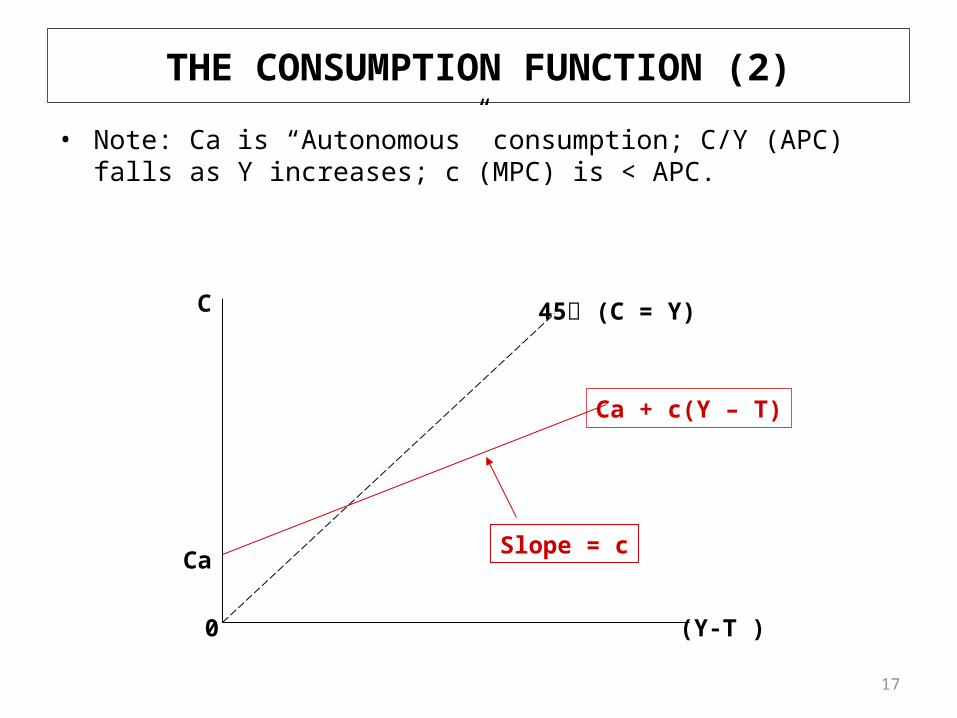
THE CONSUMPTION FUNCTION (2)

• Note: Ca is “Autonomous” consumption; C/Y (APC) falls as Y increases; c (MPC) is < APC.

0 (Y-T )

C

Ca

Ca + c(Y – T)

45 (C = Y)

Slope = c

18

• As always equilibrium is where plans are consistent• Specifically in this case planned production is equal to planed demand

Y = PE,• Sub in equation for planned expenditure (“Aggregate Demand”)

PE = C + I + G + NX• To get Y = C + I + G + NX• Sub in consumption function• To get: Y = Ca + cY – cT + Ip + G + NX• Note

– cY is the one part of Expenditure which depends on Income– The other components (Ca –cT + I + G + NX) may be termed autonomous planned

spending, in that they do not depend in Income (at least for now…)• Alternatively we might term them the Endogenous and Exogenous

components of planned spending.

Equilibrium

19

• We have an accounting identity: Y = C + I + G + NX

• This different from the equilibrium condition• The equilibrium condition describes planned magnitudes

– These plans may or may not be realised• The identity describes what actually happens

– This may or may not have been what was planned• Thus the equilibrium condition is true only for certain values of the

variables• The identity is true always

– Best thought of as an account rule

Eqm. Vs Idenitity

20

DISEQUILIBRIUM• To illustrate the concept of equilibrium consider a numerical example

– Suppose we have Ca = 50, c = 0.8, T = 150, I = 40, G = 150, NX = 60

• Suppose we have Y = 600• Is Income at equilibrium?• Calculate Planned expenditure (Aggregate Demand)

– PE = Ca + c(Y – T) + I + G + NX– = 50 + 0.8(450) + 40 + 150 + 60– 300 + 360 = 660

• So Planned Production (Y) < Planned Expenditure (PE)– Somebody’s plans will not be realised– Production is not sufficient to meet demand

21

Disequilibrium• Plans must be updated

– How?– We will assume that production will be increased to meet demand– Note we assume prices don’t change– Will provide empirical evidence later

• Note this is a key assumption– We will spend much of the course looking at how plans are

updated– This will depend on expectations and timeframe (LO 3)– In this simple model we assumes that plans cannot be

updated by changing prices– This turns out to be valid in the short term but not in the

long term

22

EQUILIBRIUM

• What is Equilibrium Y in this case?• We could try by trial and error• Or we could solve the equations• By definition equilibrium is where planned production equals planned

expenditure:Y = PEY = Ca + c(Y – T) + I + G + NX

Y – cY = Ca – cT + I + G + NX Y(1-c) = Ca – cT + I + G + NX Y(1 – c) = PA

• Where PA = Autonomous planned spending = Ca – cT + I + G + NX • Plug in numbers

– Y = PA/(1 –c) = (50-120+40+150+60)/(0.2) = 180/0.2 = 900

• One can re-check by plugging in all the components of PE when Y = 900 and getting PE = 900, i.e. equilibrium

23

EQUILIBRIUM

• This can all be illustrated graphically• When PE > Y, Y < Ye hence Y rises: similarly when PE < Y…..

0 Y

Ep

Ap

PE = PA + c(Y – T)

45 (PE = Y)

Ye

24

Comment

• The process is self sustaining– If we are not at equilibrium there is an automatic adjustment process that will bring us

into equilibrium– If this were not the case no point in studying eqm

• If not at eqm we are heading there• We assume for the moment that the adjustment process works by

producers changing out put to meet demand• We also assume that prices don't change

– Seems counter intuitive – This model effectively assumes that prices are fixed

• We will – provide empirical evidence alter that this is approximately true in the short run – and spend much of the rest of the course discussing when and how it isnt true

25

A CHANGE IN AGGREGATE SPENDING (1)

• Suppose Ip and therefore PA fall by 40, Ye1 falls to Ye2 by a multiple of 40 (Ye > PA)

0 Y

Ep

PA1

PE1 = PA1 + c(Y – T)

45 (PE = Y)

Ye1

PE2 = PA2 + c(Y – T)

PA2

Ye2

26

A CHANGE IN AGGREGATE SPENDING (2)

• Initial Equilibrium is: Y1 = PA1 + c(Y1 – T)

• Following Shock to PA: Y2 = PA2 + c(Y2 – T)

• Subtracting: Y2 – Y1 = PA2 – PA1 + c(Y2 – Y1)• i.e. Y = PA + c Y • so Y(1 – c) = PA • And thus: Y/PA = 1/(1 – c) or 1/s • So if c = 0.8, s = 0.2, multiplier = 5: etc….• Intuitively: an increase in PA (say G) is spent: it becomes income to someone

who re-spends c times the increase, etc…• Y = G(1 + c + c2 + c3 + ….. + cn)• cY = G(c c2 c3 + ….. + cn+1) then adding• And Y(1 c) =G(1) (the other terms cancel)• So Y/G = 1/(1-c)• You should have seen this before . If note review it in your fits year book or in

Mankiw

27

CHANGES IN SAVINGS, TAXES

• In the previous example, an increase in G of 100 produced an increase of 500 in Y.

• As T is given this means that (Y – T) increased by 500, and C increased by c.Y so savings increased by s.Y = 100

• Financing the increased G by selling Bonds to Savers?? • Now what happens if T were reduced by 100 instead of increasing G?• Initial Equilibrium is: Y1 = PA + c(Y1 – T1)• Following cut in T: Y2 = PA + c(Y2 – T2)• i.e. Y = c.Y – c.T• So Y(1 – c) = – c.T• Y/ T = – c/(1 – c) • Thus if c = 0.2, –c/(1 – c) = – 0.8/0.2 = – 4. • Note sign, magnitude (intuition of this)

28

Conclusions

1. Understand the concept of the National Income Identities– Accounting rule so true by definition for all values

2. Understand the definition of Unemployment– NILF vs U

3. Understand the definition of a price index– CPI inflation biased upwards

4. Understand the concept of Economic equilibrium and how it is influenced by expectations– Plans are consistent– What adjusts when plans are not consistent?

29

What’s Next?

• We will spend the rest of the course expanding on L.O. 4– We will add more detailed accounts of how plans are

formed– Progressively more complicated models– We will also carefully consider what adjusts when

plans are inconsistent• Next topic provides more detail on how

consumption and investment plans are made specifically we take into account interest rates.