a short summary of sequences and seriespersonal.kent.edu/~jalexopo/miscellaneous topics/summary...
TRANSCRIPT

A SHORT SUMMARY OF SEQUENCES AND SERIES
by John Alexopoulos
Last updated on October 21st, 2005

Contents
1 Sequences 3
1.1 Definitions, notation and examples . . . . . . . . . . . . . . . . . . . . . . . . . . . . . . . . . . . . . . 3
1.2 More definitions and terms . . . . . . . . . . . . . . . . . . . . . . . . . . . . . . . . . . . . . . . . . . 3
1.3 Some important theorems and facts . . . . . . . . . . . . . . . . . . . . . . . . . . . . . . . . . . . . . 5
2 Series 6
2.1 Definitions, terminology and basic examples . . . . . . . . . . . . . . . . . . . . . . . . . . . . . . . . . 6
2.2 Computing sums of infinite series . . . . . . . . . . . . . . . . . . . . . . . . . . . . . . . . . . . . . . . 6
2.2.1 Computing sums of geometric series. Some examples. . . . . . . . . . . . . . . . . . . . . . . . 7
2.3 Convergence and divergence of three important classes of series . . . . . . . . . . . . . . . . . . . . . . 9
2.4 Tests for the convergence or divergence of series. What the theorems say and what they don’t . . . . . 10
2.4.1 The test for divergence . . . . . . . . . . . . . . . . . . . . . . . . . . . . . . . . . . . . . . . . . 10
2.4.2 The Integral Test . . . . . . . . . . . . . . . . . . . . . . . . . . . . . . . . . . . . . . . . . . . . 11
2.4.3 Cauchy’s Condensation Test . . . . . . . . . . . . . . . . . . . . . . . . . . . . . . . . . . . . . . 11
2.4.4 The Comparison Test . . . . . . . . . . . . . . . . . . . . . . . . . . . . . . . . . . . . . . . . . 12
2.4.5 The limit comparison test . . . . . . . . . . . . . . . . . . . . . . . . . . . . . . . . . . . . . . . 13
2.4.6 The alternating series test . . . . . . . . . . . . . . . . . . . . . . . . . . . . . . . . . . . . . . . 14
2.4.7 Absolute and conditional convergence of series . . . . . . . . . . . . . . . . . . . . . . . . . . . 14
2.4.8 The ratio test . . . . . . . . . . . . . . . . . . . . . . . . . . . . . . . . . . . . . . . . . . . . . . 15
2.4.9 The root test . . . . . . . . . . . . . . . . . . . . . . . . . . . . . . . . . . . . . . . . . . . . . . 16
1

3 Power series 17
3.1 Definitions and basic concepts . . . . . . . . . . . . . . . . . . . . . . . . . . . . . . . . . . . . . . . . . 17
3.2 Some important facts . . . . . . . . . . . . . . . . . . . . . . . . . . . . . . . . . . . . . . . . . . . . . 18
3.3 Taylor and Maclaurin series . . . . . . . . . . . . . . . . . . . . . . . . . . . . . . . . . . . . . . . . . . 19
3.4 Computing sums of series using power series techniques . . . . . . . . . . . . . . . . . . . . . . . . . . 22
2

Chapter 1
Sequences
1.1 Definitions, notation and examples
A sequence is a function whose domain is the set of positive (or the non–negative) integers. If a denotes such an
object, and n is a positive integer, we write a(n) = an and we denote the sequence a itself by a = {an} .
Examples:{
1n
},{(
23
)n},{
12 , 2
3 , 34 , 4
5 , . . . , nn+1 , . . .
}, {0, 2, 0, 2, . . .} are all examples of sequences.
We can talk about limits of sequences as n tends to infinity. If {an} is a sequence, we denote its limit by limn→∞ an
or simply lim an. If lim an exists (in a finite sense) we say that the sequence {an} is a convergent sequence. Otherwise
we say that the sequence {an} is divergent. In the special case of lim an = 0, we say that the (convergent) sequence
{an} is null.
Examples:
1.{
12 , 2
3 , 34 , 4
5 , . . . , nn+1 , . . .
}is an example of a convergent sequence since lim n
n+1 = 1.
2.{
1n
},{(
23
)n} are examples of null sequences since lim 1n = 0 and lim
(23
)n = 0.
3. {0, 2, 0, 2, . . .} , {(−1)n} , {en} are all examples of divergent sequences since their limits do not exist.
1.2 More definitions and terms
1. We now give the definition of the limit of a sequence:
3

lim an = L if and olny if for every ε > 0 there is a positive integer N such that |an − L| < ε whenever n ≥ N .
2. We say that a sequence {an} satisfies a given property eventually if there is a positive integer N such that
the given property is satisfied for all terms an for which n ≥ N. That is, the given property is satisfied for all
but finitely many terms of the sequence. As an example of the usage of the word “eventually”, refer to the
definition of the limit which can be reformulated as follows:
lim an = L if and olny if for every ε > 0, |an − L| < ε eventually.
3. We say that a sequence {an} is increasing if an ≤ an+1 for all n.
We say that a sequence {an} is decreasing if an ≥ an+1 for all n.
In any of these cases we say that {an} is monotonic.
4. We say that a sequence {an} is bounded if there is a positive number M such that |an| ≤ M for all n.
Examples:
1. We will use the definition of the limit to establish the following:
(a) lim(
3n+12n+5
)= 3
2 : Let ε > 0 and choose a positive integer N such that N > 134ε . Then
n ≥ N =⇒ n >134ε
=⇒ 134n
< ε =⇒ 134n + 10
<134n
< ε =⇒∣∣∣∣ −134n + 10
∣∣∣∣ < ε
=⇒∣∣∣∣6n− 6n + 2− 15
4n + 10
∣∣∣∣ < ε =⇒∣∣∣∣2 (3n + 1)− 3 (2n + 5)
2 (2n + 5)
∣∣∣∣ < ε
=⇒∣∣∣∣3n + 12n + 5
− 32
∣∣∣∣ < ε
and so lim(
3n+12n+5
)= 3
2 by definition.
(b) lim(
n2−12n2+3
)= 1
2 : Let ε > 0 and choose a positive integer N such that N > 2√5ε
. Then
n ≥ N =⇒ n >
√5
2√
ε=⇒
√5
n< 2
√ε =⇒ 5
n2< 4ε =⇒ 5
4n2< ε
=⇒ 54n2 + 6
<5
4n2< ε =⇒
∣∣∣∣ −52 (2n2 + 3)
∣∣∣∣ < ε =⇒∣∣∣∣2n2 − 2− 2n2 − 3
2 (2n2 + 3)
∣∣∣∣ < ε
=⇒
∣∣∣∣∣2(n2 − 1
)−(2n2 + 3
)2 (2n2 + 3)
∣∣∣∣∣ < ε =⇒∣∣∣∣ n2 − 12n2 + 3
− 12
∣∣∣∣ < ε
and so lim(
n2−12n2+3
)= 1
2 by definition.
4
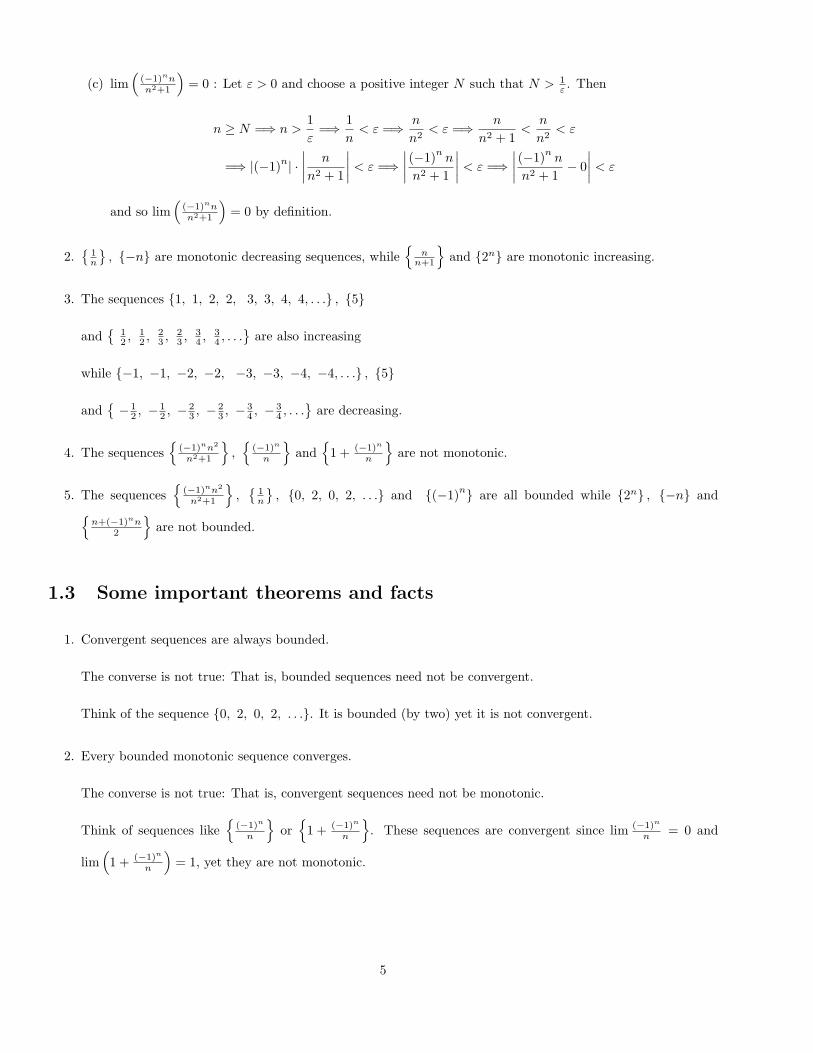
(c) lim(
(−1)nnn2+1
)= 0 : Let ε > 0 and choose a positive integer N such that N > 1
ε . Then
n ≥ N =⇒ n >1ε
=⇒ 1n
< ε =⇒ n
n2< ε =⇒ n
n2 + 1<
n
n2< ε
=⇒ |(−1)n| ·∣∣∣∣ n
n2 + 1
∣∣∣∣ < ε =⇒∣∣∣∣ (−1)n
n
n2 + 1
∣∣∣∣ < ε =⇒∣∣∣∣ (−1)n
n
n2 + 1− 0∣∣∣∣ < ε
and so lim(
(−1)nnn2+1
)= 0 by definition.
2.{
1n
}, {−n} are monotonic decreasing sequences, while
{n
n+1
}and {2n} are monotonic increasing.
3. The sequences {1, 1, 2, 2, 3, 3, 4, 4, . . .} , {5}
and{
12 , 1
2 , 23 , 2
3 , 34 , 3
4 , . . .}
are also increasing
while {−1, −1, −2, −2, −3, −3, −4, −4, . . .} , {5}
and{− 1
2 , − 12 , − 2
3 , − 23 , − 3
4 , − 34 , . . .
}are decreasing.
4. The sequences{
(−1)nn2
n2+1
},{
(−1)n
n
}and
{1 + (−1)n
n
}are not monotonic.
5. The sequences{
(−1)nn2
n2+1
},{
1n
}, {0, 2, 0, 2, . . .} and {(−1)n} are all bounded while {2n} , {−n} and{
n+(−1)nn2
}are not bounded.
1.3 Some important theorems and facts
1. Convergent sequences are always bounded.
The converse is not true: That is, bounded sequences need not be convergent.
Think of the sequence {0, 2, 0, 2, . . .}. It is bounded (by two) yet it is not convergent.
2. Every bounded monotonic sequence converges.
The converse is not true: That is, convergent sequences need not be monotonic.
Think of sequences like{
(−1)n
n
}or{
1 + (−1)n
n
}. These sequences are convergent since lim (−1)n
n = 0 and
lim(1 + (−1)n
n
)= 1, yet they are not monotonic.
5

Chapter 2
Series
2.1 Definitions, terminology and basic examples
Let {an} be a sequence. For each positive integer n define sn = a1 + a2 + · · · + an or more concisely written
sn =∑n
k=1 ak. The sequence of partial sums {sn} is called an infinite series and it is denoted by∑∞
n=1 an or simply∑an. The sequence {an} is called the sequence of terms of the series
∑an.
Example:∑
1n =
{1, 1 + 1
2 , 1 + 12 + 1
3 , . . . ,∑n
k=11k , . . .
}is an infinite series. The sequence
{1n
}={1, 1
2 , 13 , 1
4 , . . . , 1n , . . .
}is the sequence of terms of this series.
∑1n is a special series called the harmonic series.
Convergent and Divergent series: Since after all series are sequences, it makes sense to ask whether or not they
converge or diverge. That is, if lim sn = limn→∞∑n
k=1 ak exists (in the finite sense) then we say that∑
an is
convergent. Otherwise we say that∑
an diverges. If a series converges then the value s = lim sn = limn→∞∑n
k=1 ak
is called the sum of the series and it is denoted (watch out!) by s =∑∞
n=1 an . In most instances, the context
determines whether the meaning of the symbol∑∞
n=1 an refers to the series itself or its sum.
2.2 Computing sums of infinite series
Computing the sum of a (convergent) series is in general a hard task. Nevertheless it is reasonably easy for the
following two cases:
6
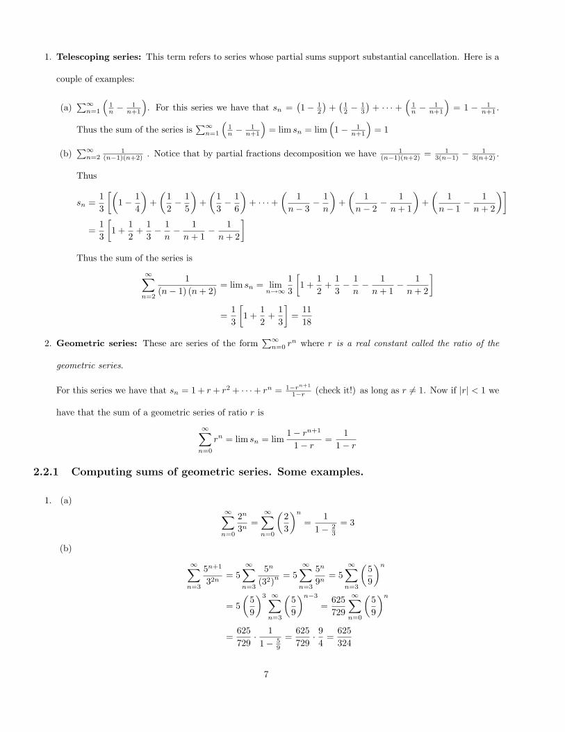
1. Telescoping series: This term refers to series whose partial sums support substantial cancellation. Here is a
couple of examples:
(a)∑∞
n=1
(1n −
1n+1
). For this series we have that sn =
(1− 1
2
)+(
12 −
13
)+ · · · +
(1n −
1n+1
)= 1 − 1
n+1 .
Thus the sum of the series is∑∞
n=1
(1n −
1n+1
)= lim sn = lim
(1− 1
n+1
)= 1
(b)∑∞
n=21
(n−1)(n+2) . Notice that by partial fractions decomposition we have 1(n−1)(n+2) = 1
3(n−1) −1
3(n+2) .
Thus
sn =13
[(1− 1
4
)+(
12− 1
5
)+(
13− 1
6
)+ · · ·+
(1
n− 3− 1
n
)+(
1n− 2
− 1n + 1
)+(
1n− 1
− 1n + 2
)]=
13
[1 +
12
+13− 1
n− 1
n + 1− 1
n + 2
]Thus the sum of the series is
∞∑n=2
1(n− 1) (n + 2)
= lim sn = limn→∞
13
[1 +
12
+13− 1
n− 1
n + 1− 1
n + 2
]
=13
[1 +
12
+13
]=
1118
2. Geometric series: These are series of the form∑∞
n=0 rn where r is a real constant called the ratio of the
geometric series.
For this series we have that sn = 1 + r + r2 + · · ·+ rn = 1−rn+1
1−r (check it!) as long as r 6= 1. Now if |r| < 1 we
have that the sum of a geometric series of ratio r is
∞∑n=0
rn = lim sn = lim1− rn+1
1− r=
11− r
2.2.1 Computing sums of geometric series. Some examples.
1. (a)∞∑
n=0
2n
3n=
∞∑n=0
(23
)n
=1
1− 23
= 3
(b)
∞∑n=3
5n+1
32n= 5
∞∑n=3
5n
(32)n = 5∞∑
n=3
5n
9n= 5
∞∑n=3
(59
)n
= 5(
59
)3 ∞∑n=3
(59
)n−3
=625729
∞∑n=0
(59
)n
=625729
· 11− 5
9
=625729
· 94
=625324
7

(c) The following technique is called summation by parts. It is similar to the “cyclic” integration by parts:
i.
∞∑n=1
n
2n=
12
+222
+323
+ · · ·
=(
12
+122
+123
+ · · ·)
+(
122
+223
+324
+ · · ·)
=∞∑
n=1
12n
+∞∑
n=1
n
2n+1=
12
∞∑n=1
12n−1
+12
∞∑n=1
n
2n
=12
∞∑n=0
12n
+12
∞∑n=1
n
2n=
12· 11− 1
2
+12
∞∑n=1
n
2n
= 1 +12
∞∑n=1
n
2n
Thus if x =∑∞
n=1n2n we have that x = 1 + 1
2x and so x =∑∞
n=1n2n = 2.
ii. Compute the sum of the series∑∞
n=1n23n
5n+1 :
First notice that∞∑
n=1
n23n
5n+1=
12 · 352
+∞∑
n=2
n23n
5n+1=
325
+∞∑
n=2
n23n
5n+1
Furthermore
∞∑n=2
n23n
5n+1=
∞∑n=1
(n + 1)2 3n+1
5n+2=
35
∞∑n=1
(n2 + 2n + 1
)3n
5n+1
=35
[ ∞∑n=1
n23n
5n+1+ 2
∞∑n=1
n3n
5n+1+
∞∑n=1
3n
5n+1
]
=35
[ ∞∑n=1
n23n
5n+1+ 2
∞∑n=1
n3n
5n+1+
325
∞∑n=1
3n−1
5n−1
]
=35
[ ∞∑n=1
n23n
5n+1+ 2
∞∑n=1
n3n
5n+1+
325
∞∑n=0
3n
5n
]
=35
[ ∞∑n=1
n23n
5n+1+ 2
∞∑n=1
n3n
5n+1+
325· 11− 3
5
]
=35
[ ∞∑n=1
n23n
5n+1+ 2
∞∑n=1
n3n
5n+1+
310
]
8
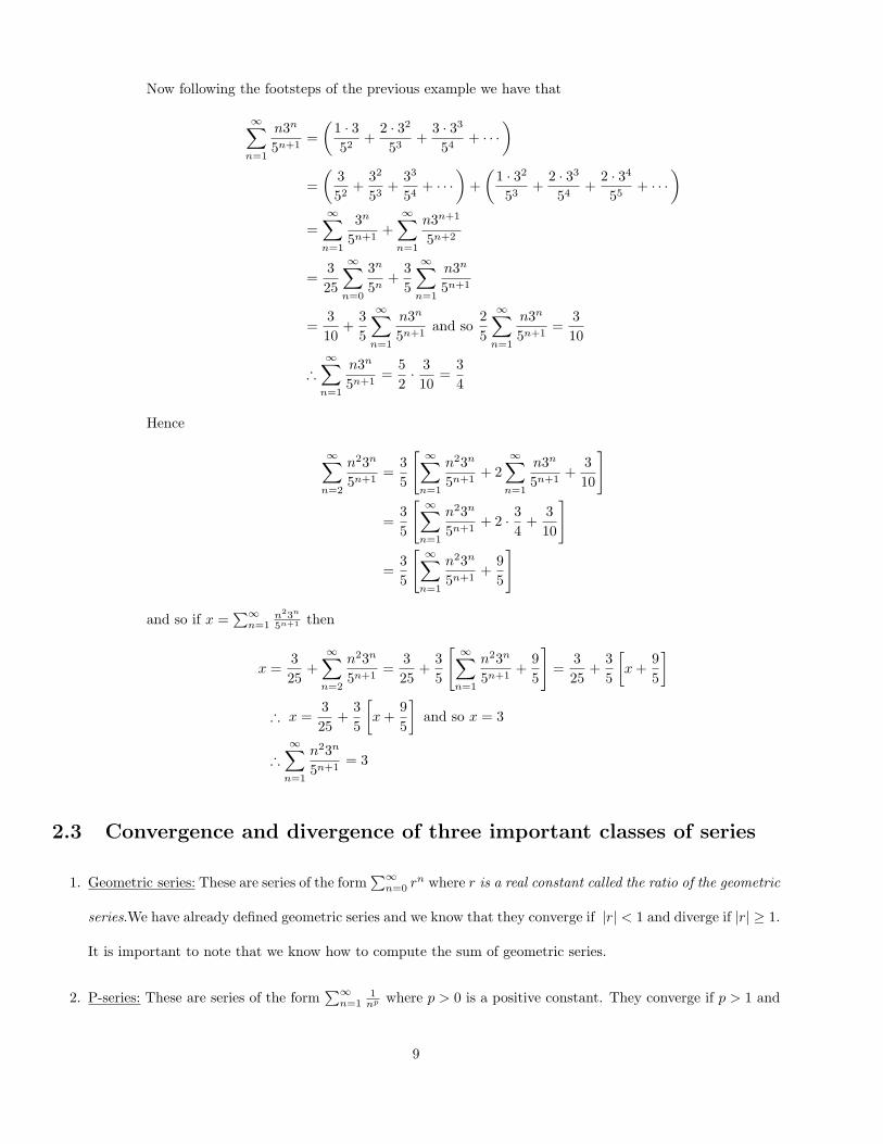
Now following the footsteps of the previous example we have that
∞∑n=1
n3n
5n+1=(
1 · 352
+2 · 32
53+
3 · 33
54+ · · ·
)
=(
352
+32
53+
33
54+ · · ·
)+(
1 · 32
53+
2 · 33
54+
2 · 34
55+ · · ·
)=
∞∑n=1
3n
5n+1+
∞∑n=1
n3n+1
5n+2
=325
∞∑n=0
3n
5n+
35
∞∑n=1
n3n
5n+1
=310
+35
∞∑n=1
n3n
5n+1and so
25
∞∑n=1
n3n
5n+1=
310
∴∞∑
n=1
n3n
5n+1=
52· 310
=34
Hence
∞∑n=2
n23n
5n+1=
35
[ ∞∑n=1
n23n
5n+1+ 2
∞∑n=1
n3n
5n+1+
310
]
=35
[ ∞∑n=1
n23n
5n+1+ 2 · 3
4+
310
]
=35
[ ∞∑n=1
n23n
5n+1+
95
]
and so if x =∑∞
n=1n23n
5n+1 then
x =325
+∞∑
n=2
n23n
5n+1=
325
+35
[ ∞∑n=1
n23n
5n+1+
95
]=
325
+35
[x +
95
]
∴ x =325
+35
[x +
95
]and so x = 3
∴∞∑
n=1
n23n
5n+1= 3
2.3 Convergence and divergence of three important classes of series
1. Geometric series: These are series of the form∑∞
n=0 rn where r is a real constant called the ratio of the geometric
series.We have already defined geometric series and we know that they converge if |r| < 1 and diverge if |r| ≥ 1.
It is important to note that we know how to compute the sum of geometric series.
2. P-series: These are series of the form∑∞
n=11
np where p > 0 is a positive constant. They converge if p > 1 and
9

they diverge if p ≤ 1. In order to see this apply the integral test or Cauchy’s Condensation Test (see below).
It is worth noting that the harmonic series is a p-series with p = 1.
3. Log-p-series: These are series of the form∑∞
n=11
n(ln n)p where p > 0 is a positive constant. They converge if
p > 1 and they diverge if p ≤ 1. In order to see this apply the integral test or Cauchy’s Condensation Test
(see below).
2.4 Tests for the convergence or divergence of series. What the theo-
rems say and what they don’t
2.4.1 The test for divergence
What does the theorem say:
All three of the following statements are true and logically equivalent to each other:
1. If∑
an converges then lim an = 0
2. If∑
an converges then {an} , the sequence of terms of the series, is null.
3. If {an} is not a null sequence (i.e. lim an 6= 0) then∑
an diverges.
Examples:
1. Suppose that the series∑
2nwn is convergent. What can you say about the sequence of terms {2nwn}?
Well... {2nwn} is a null sequence. That is lim 2nwn = 0.
2. Suppose that lim 2nwn = 0. What can you say about the convergence or divergence of∑
2nwn ?
Absolutely NOTHING. We simply don’t have enough information to decide.
3. Does the series∑
(−1)n n2n+1 converge or diverge?
Well... it diverges because lim n2n+1 = 1
2 and thus lim (−1)n n2n+1 does not exist. In particular the sequence{
(−1)n n2n+1
}is not a null sequence.
10

Common abuses: The theorem NEVER claimed the convergence of∑
an whenever lim an = 0. Such a statement
is plainly false.
Just consider the harmonic series∑
1n : We know that this series diverges YET lim 1
n = 0
2.4.2 The Integral Test
What does the theorem say:
Suppose that f is (eventually) decreasing continuous and positive. Then∫∞
mf(x)dx converges if and only if∑∞
n=m f(n) converges.
In other words∫∞
mf(x)dx and
∑∞n=m f(n) either both converge or both diverge.
Example: The integral test is utilized to determine the convergence or divergence of p-series and log-p-series. Once
these facts are established the Integral Test has a limited use one reason being that integration is not always easy
(or even possible).
Common abuses:
People often times forget to check the hypotheses of the theorem. In particular make sure that you check that f is
decreasing. In non–obvious cases a sign–chart for the derivative of f is just what the doctor ordered.
2.4.3 Cauchy’s Condensation Test
What does the theorem say:
Let {an} be an (eventually) decreasing positive sequence. Then∑
an converges if and only if∑
2na2n converges.
In other words∑
an and∑
2na2n either both converge or both diverge.
Examples: Cauchy’s condensation test provides in many instances a cleaner alternative to the Integral Test. For
example lets see how this test treats p-series and log-p-series:
1. Consider the p-series∑
1np and use the condensation test to obtain the series
∑2n · 1
(2n)p =∑
2n
(2p)n =∑(
22p
)n.
If 0 < p ≤ 1 then 2p ≤ 2 and thus 22p ≥ 1 and so the geometric series
∑(22p
)n diverges. On the other hand if
p > 1 then 2p > 2 and so 22p < 1 making the geometric series
∑(22p
)n convergent.
2. Consider the log-p-series∑
1n(ln n)p and use the condensation test to obtain the series
∑2n · 1
2n(n ln 2)p =∑1
np(ln 2)p = 1(ln 2)p
∑1
np . This series is a non–zero constant multiple of a p-series and thus it converges if
11

p > 1 and it diverges for 0 < p ≤ 1.
Common abuses: Just like in the integral test make sure that the hypotheses are satisfied. In particular ensure
that the sequence {an} is (eventually) decreasing.
2.4.4 The Comparison Test
What does the theorem say:
Let {an} and {bn} be two sequences of non–negative terms and suppose that (eventually) an ≤ bn. The following
statements are true:
1. If∑
bn is convergent then so is∑
an
2. If∑
an is divergent then so is∑
bn
The comparison test is the “work–horse” of all tests. Its use depends on prior knowledge of the behavior of certain
series.
Examples:
1. Determine whether or not∑
n−1n3+n+1 converges or diverges.
Notice that n−1n3+n+1 < n
n3+n+1 < nn3 = 1
n2 .
We know that∑
1n2 converges (p-series p = 2 > 1). Hence so does
∑n−1
n3+n+1 thanks to the comparison test.
2. Determine whether or not∑∞
n=2n
n2−n−1 converges or diverges.
Notice that nn2−n−1 > n
n2 = 1n .
We know that∑
1n diverges (harmonic series). Hence so does
∑∞n=2
nn2−n−1 thanks to the comparison test.
3. Determine whether or not∑∞
n=2n
n3−n2−1 converges or diverges.
Here the inequalities do not work in our favor. But we know that the sequence{
nn3−n2−1
}behaves essentially
like{
1n2
}. Based on this observation we can try the following argument:
nn3−n2−1 < n
n3− 12 n3 = n
12 n3 = 2n
n3 = 2n2 (eventually)
Now∑
1n2 converges (p-series p = 2 > 1). Hence
∑2
n2 = 2∑
1n2 converges and thus so does
∑∞n=2
nn3−n2−1
by the comparison test.
12

Common abuses: Careful: the inequalities must be just right and they should be going the “right way”. For
instance, one could be tempted to do the following on example (3):
nn3−n2−1 > n
n3 = 1n2 . Even though
∑1
n2 converges we can conclude NOTHING about the behavior of∑∞
n=2n
n3−n2−1 .
2.4.5 The limit comparison test
What does the theorem say:
Let {an} and {bn} be two sequences of positive terms and let lim an
bn= L.
1. If L 6= 0 and L < ∞ then∑
an and∑
bn either both converge or both diverge.
That is,∑
an if and only if∑
bn converges.
2. If L = 0 and∑
bn converges then so does∑
an.
3. If L = 0 and∑
an diverges then so does∑
bn.
4. If L = ∞ and∑
an converges then so does∑
bn.
5. If L = ∞ and∑
bn diverges then so does∑
an.
The most commonly used part is part (1). I suggest that you don’t memorize parts (2)–(5) but if you have to,
rather think that if lim an
bn= 0 then eventually an < bn and if lim an
bn= ∞ then eventually an > bn. Then use the
comparison test.
The limit comparison test is especially useful in situations like in example (3) of the previous section.
Examples:
1. Determine whether or not∑∞
n=2n
n3−n2−1 converges or diverges.
Lets use the limit comparison test with∑
1n2 :
limn
n3−n2−11
n2= lim n
n3−n2−1 ·n2
1 = lim n3
n3−n2−1 = lim 11− 1
n−1
n2= 1
Since∑
1n2 converges (p-series p = 2 > 1) then so does
∑∞n=2
nn3−n2−1 thanks to the limit comparison test.
2. Determine whether or not∑
1
n1+ 1n
converges or diverges.
Use the limit comparison test with the harmonic series∑
1n :
13

lim1
n1+ 1
n1n
= lim n
n1+ 1n
= lim 1
n1n
= 1
We know that∑
1n diverges (harmonic series). Hence so does
∑1
n1+ 1n
thanks to the limit comparison test.
2.4.6 The alternating series test
So far all are tests for convergence of series dealt with series of non–negative terms. In this section we take a look at
a special kind of series whose sequence of terms “alternates” from positive to negative or vice–versa:
Definition: Let {an} be a sequence of positive terms (i.e. an > 0). The series∑
(−1)nan is called an alternating
series.
What does the theorem say:
Let {an} be a decreasing, null sequence of positive terms (i.e. {an} decreases, an > 0 and lim an = 0). Then the
alternating series∑
(−1)nan converges.
Examples:∑(−1)n 1
n ,∑
(−1)n 1ln n ,
∑(−1)n ( 1
n!
)are all convergent series thanks to the alternating series test.
Common abuses: Just like in the integral test and Cauchy’s condensation test make sure that the hypotheses are
satisfied. In particular ensure that the sequence {an} is (eventually) decreasing.
2.4.7 Absolute and conditional convergence of series
Definition: If the series∑|an| converges then the series
∑an is called absolutely convergent.
If the series∑|an| diverges and the series
∑an converges then the series
∑an is called conditionally convergent.
Some facts:
1. Absolutely convergent series are always convergent.
2. It follows from the statement above that if∑
an diverges then so does∑|an|.
Examples:
1.∑
(−1)n 1n is a conditionally convergent series because
∑(−1)n 1
n converges (alternating series test)
yet∑∣∣(−1)n 1
n
∣∣ =∑ 1n diverges (harmonic series).
14

2.∑ (−1)n
n3 is an absolutely convergent series because∑∣∣∣ (−1)n
n3
∣∣∣ =∑ 1n3 converges (p-series p = 2 > 1).
2.4.8 The ratio test
What does the theorem say:
Let {an} be a sequence of (eventually) non–zero terms (i.e. eventually an 6= 0) and let lim∣∣∣an+1
an
∣∣∣ = L. Then
1. If L < 1 then∑
an is absolutely convergent.
2. If L > 1 then∑
an is divergent.
3. If L = 1 then no conclusions can be drawn from this test.
Examples:
1.∑
1n! is (absolutely) convergent:
lim1
(n+1)!1n!
= lim n!(n+1)! = lim 1
n = 0 < 1
So∑
1n! is (absolutely) convergent by the ratio test
2.∑
2nn!nn is (absolutely) convergent:
lim2n+1(n+1)!
(n+1)n+1
2nn!nn
= lim2n+1 (n + 1)!(n + 1)n+1 · nn
2nn!= lim 2 · nn
(n + 1)n
= 2 lim(
n
n + 1
)n
= 2 lim1(
n+1n
)n= 2 lim
1(1 + 1
n
)n =2e
< 1
So∑
2nn!nn is (absolutely) convergent by the ratio test.
3.∑
n!10n diverges:
lim(n+1)!10n+1
n!10n
= lim (n+1)!10n+1
10n
n! = lim n+110 = ∞ > 1
So∑
n!10n diverges by the ratio test.
15

2.4.9 The root test
What does the theorem say:
Let {an} be a sequence of terms and let lim n√|an| = lim |an|
1n = L. Then
1. If L < 1 then∑
an is absolutely convergent.
2. If L > 1 then∑
an is divergent.
3. If L = 1 then no conclusions can be drawn from this test.
Examples:
1.∑
rn
nn is (absolutely) convergent for any constant r:
lim n
√∣∣ rn
nn
∣∣ = lim |r|n = 0 < 1
∴∑
rn
nn is (absolutely) convergent for any constant r, by the root test.
2.∑
nprn is (absolutely) convergent for any constants r with |r| < 1 and p > 0:
lim n√|nprn| = lim |r| ( n
√n)p = |r| < 1
∴∑
nprn is (absolutely) convergent for any constants r with |r| < 1 and p > 0 thanks to the root test.
Comments about the ratio and root tests: Even though the ratio and root tests appear to be very powerful they
are nothing more but fancy comparison tests to geometric series. Consequently these tests will yield no information
when they are used to determine the behavior of p-series or log-p-series (try it!). Their utility becomes more apparent
in the study of power–series.
16
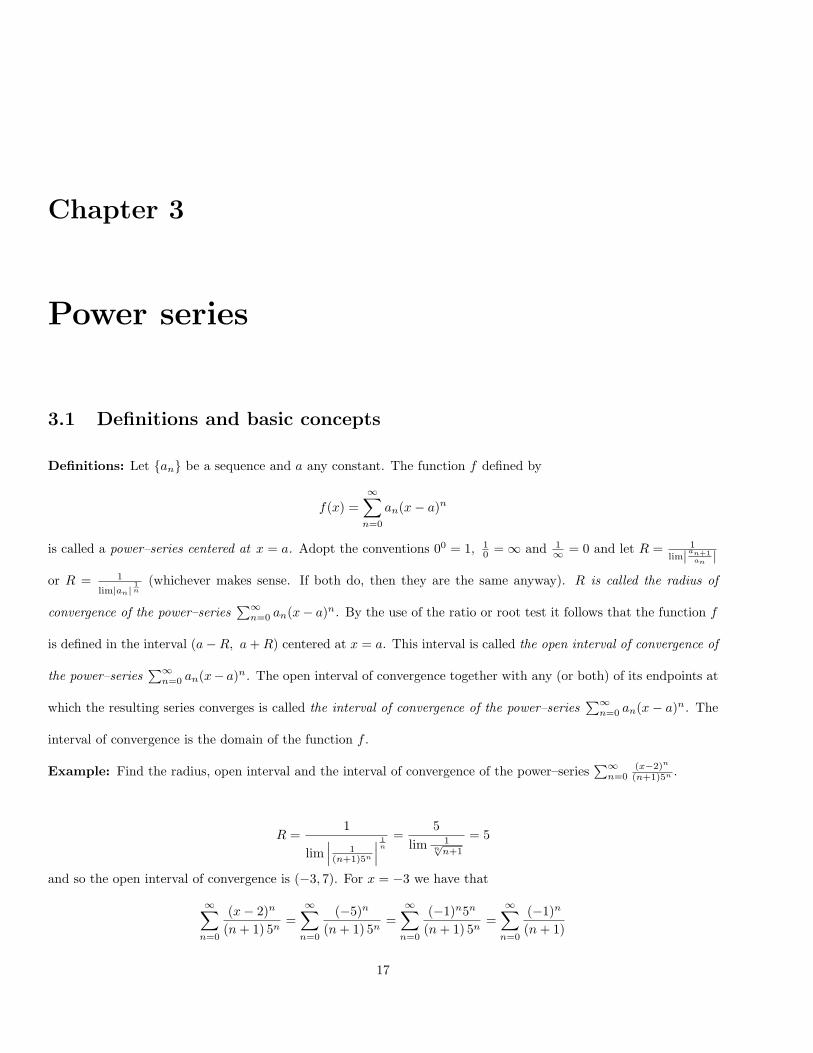
Chapter 3
Power series
3.1 Definitions and basic concepts
Definitions: Let {an} be a sequence and a any constant. The function f defined by
f(x) =∞∑
n=0
an(x− a)n
is called a power–series centered at x = a. Adopt the conventions 00 = 1, 10 = ∞ and 1
∞ = 0 and let R = 1
lim| an+1an
|
or R = 1
lim|an|1n
(whichever makes sense. If both do, then they are the same anyway). R is called the radius of
convergence of the power–series∑∞
n=0 an(x− a)n. By the use of the ratio or root test it follows that the function f
is defined in the interval (a−R, a + R) centered at x = a. This interval is called the open interval of convergence of
the power–series∑∞
n=0 an(x− a)n. The open interval of convergence together with any (or both) of its endpoints at
which the resulting series converges is called the interval of convergence of the power–series∑∞
n=0 an(x− a)n. The
interval of convergence is the domain of the function f .
Example: Find the radius, open interval and the interval of convergence of the power–series∑∞
n=0(x−2)n
(n+1)5n .
R =1
lim∣∣∣ 1(n+1)5n
∣∣∣ 1n
=5
lim 1n√
n+1
= 5
and so the open interval of convergence is (−3, 7). For x = −3 we have that
∞∑n=0
(x− 2)n
(n + 1) 5n=
∞∑n=0
(−5)n
(n + 1) 5n=
∞∑n=0
(−1)n5n
(n + 1) 5n=
∞∑n=0
(−1)n
(n + 1)
17

which converges (by the alternating series test). For x = 7 we have that
∞∑n=0
(x− 2)n
(n + 1) 5n=
∞∑n=0
5n
(n + 1) 5n=
∞∑n=0
1n + 1
which diverges (limit compare with the harmonic series∑
1n ). Thus the interval of convergence of the power–series∑∞
n=0(x−2)n
(n+1)5n is [−3, 7).
3.2 Some important facts
1. It turns out that power–series are infinitely differentiable functions within their open interval of convergence.
Moreover their derivatives have the same open interval of convergence.
2. Power–series are differentiated and integrated term–by–term. That is
d
dx
∞∑n=0
an(x− a)n =∞∑
n=1
nan(x− a)n−1 =∞∑
n=0
(n + 1) an+1(x− a)n
and ∫ ( ∞∑n=0
an(x− a)n
)dx = C +
∞∑n=0
an
n + 1(x− a)n+1 = C +
∞∑n=1
an−1
n(x− a)n
3. If f(x) =∑∞
n=0 an(x−a)n then f (n) (a) = an · n! and thus an = f(n)(a)n! . This means that if an infinite differ-
entiable function can be expressed as a power series centered at x = a then such a power series representation
is unique. That is, for x in the open interval of convergence f(x) =∑∞
n=0f(n)(a)
n! (x− a)n.
Examples:
(a) If f(x) = ex then for each n we know that f (n) (x) = ex and so f (n) (0) = 1. Hence if f can be expressed
as a power–series centered at x = 0 this series has no choice but be∑∞
n=0xn
n! . In fact, we will see later
that ex =∑∞
n=0xn
n! for all x.
(b) If f(x) = 11−x then we know that for each x in (−1, 1), f(x) =
∑∞n=0 xn. Thus f (n) (0) = n!
One may ask what is f (n) (3) ? Well...here is some magic:
f(x) =1
1− x=
11− x + 3− 3
=1
−2− (x− 3)=
−12 + (x− 3)
=−12
1 + (x−3)2
= −12· 11 + 1
2 (x− 3)
= −12
∞∑n=0
(−1
2(x− 3)
)n
= −12
∞∑n=0
(−1)n
2n(x− 3)n =
∞∑n=0
(−1)n+1
2n+1(x− 3)n
18

By the uniqueness of such representation we conclude that f (n) (3) = (−1)n+1
2n+1 · n!
(c) Let f(x) =∑∞
n=0n+12n (x− 1)3n+1. Then notice that
i. f(1) = 0
ii. f (1)(1) = 1 ( 3n + 1 = 1 when n = 0, and the coefficient n+12n
∣∣n=0
= 1)
iii. f (2)(1) = 0 (3n + 1 6= 2 and so the coefficient of (x− 1)2 MUST be 0.)
iv. f (3)(1) = 0 (3n + 1 6= 3 and so the coefficient of (x− 1)3 MUST be 0.)
v. f (4)(1) = 4! = 24 (3n + 1 = 4 only when n = 1 and so the coefficient of (x− 1)3 is n+12n
∣∣n=1
= 1
vi. In general
f (n)(1) =
k+12k k! = (k+1)!
2k if n = 3k + 1 for some k
0 otherwise
3.3 Taylor and Maclaurin series
Definitions:
1. Let f be infinitely differentiable at x = a. As we have seen, the only possible power–series representation of f
centered at x = a is given by∑∞
n=0f(n)(a)
n! (x − a)n. This power–series is called the Taylor series of f about
x = a.
2. If a = 0 then the power–series∑∞
n=0f(n)(0)
n! xn is called the Maclaurin series of f .
3. If f(x) =∑∞
n=0f(n)(a)
n! (x − a)n for all x in some interval centered at x = a then we say that f is analytic at
x = a
In tandem to what we mentioned in the previous section, if a function f happens to equal the power–series∑∞n=0 an(x − a)n on some interval centered at x = a then this series IS THE TAYLOR SERIES OF f ABOUT
x = a (i.e. an = f(n)(a)n! for all n).
Examples: The examples that follow are very important. You can obtain these series by direct computation of the
coefficients an = f(n)(a)n! .
19

1. We have already seen the Maclaurin series of f(x) = ex and we have already mentioned that it is actually
equal to ex for all x:
ex =∞∑
n=0
xn
n!
2. The Maclaurin series of f(x) = sin x. It too equals sinx for all x:
sinx =∞∑
n=0
(−1)n
(2n + 1)!x2n+1
3. The Maclaurin series of f(x) = cos x. It too equals cos x for all x:
cos x =∞∑
n=0
(−1)n
(2n)!x2n
There are examples of infinitely differentiable functions that DO NOT equal their Maclaurin series on any interval
containing 0. Here is one of the most commonly presented examples:
Example: The function f defined by
f(x) =
e−
1x2 if x 6= 0
0 if x = 0
is infinitely differentiable at x = 0 with f (n) (0) = 0. Hence the Maclaurin series of f is identically zero YET f(x) = 0
ONLY WHEN x = 0. In other words f is an example of an infinitely differentiable function at x = 0 that is not
analytic at x = 0.
How does one decides whether or not the Taylor series of a function actually equals the function on some interval
containing the center?
There are many possible approaches into answering this question. We are going to mention two of them.
1. Take advantage of the uniqueness of the representation. If we somehow know that f(x) =∑∞
n=0 an(x − a)n
in some open interval containing a then∑∞
n=0 an(x − a)n HAS NO CHOICE BUT TO BE THE TAYLOR
SERIES OF f ABOUT x = a (i.e. an = f(n)(a)n! for all n). Here are couple of examples:
Examples:
(a) We know that f(x) = 11−x =
∑∞n=0 xn for all x in (−1, 1). Hence
∑∞n=0 xn IS the Maclaurin series of f .
20

(b) How can we find the Maclaurin series of f(x) = arctanx and at the same time KNOW that it is equal to
f on some interval containing 0? Here is some more magic:
Notice that f ′(x) = 11+x2 . The strategy is to find the Maclaurin series and integrate term-by-term.
Well...f ′(x) = 11+x2 =
∑∞n=0
(−x2
)n =∑∞
n=0 (−1)nx2n and so
f(x) =∫ ( ∞∑
n=0
(−1)nx2n
)dx =
∞∑n=0
(−1)n
(∫x2ndx
)= C +
∞∑n=0
(−1)n x2n+1
2n + 1
Since f(0) = arctan 0 = 0 we conclude that C = 0 and thus f(x) = arctanx =∑∞
n=0 (−1)n x2n+1
2n+1 for all
x in (−1, 1). Hence IS the∑∞
n=0 (−1)n x2n+1
2n+1 Maclaurin series of f .
(c) Find the Taylor series of f(x) = lnx about x = 3 and show that it is equal to f on some interval
containing 3.
Again, the strategy is to find the Taylor series of f ′ and integrate term-by-term:
f ′(x) =1x
=1
x− 3 + 3=
13 + (x− 3)
=13· 1
1 + (x−3)3
=13
∞∑n=0
(−x− 3
3
)n
=13
∞∑n=0
(−1)n
3n(x− 3)n =
∞∑n=0
(−1)n
3n+1(x− 3)n
So
f(x) = lnx =∫ ( ∞∑
n=0
(−1)n
3n+1(x− 3)n
)dx =
∞∑n=0
(−1)n
3n+1
∫(x− 3)n
dx = C +∞∑
n=0
(−1)n
(n + 1) 3n+1(x− 3)n+1
Since f(3) = ln 3 we conclude that C = ln 3. Hence the Taylor series of f about x = 3 is ln 3 +∑∞n=0
(−1)n
(n+1)3n+1 (x− 3)n+1 and in fact f(x) = lnx = ln 3 +∑∞
n=0(−1)n
(n+1)3n+1 (x− 3)n+1 for all x in (0, 6)
(find the open interval of convergence of the resulting series!).
2. You can always directly compute the coefficients an = f(n)(a)n! , find the Taylor series and subsequently use the
Lagrange form of the remainder theorem given below, to examine whether or not the Taylor series converges
in some interval containing a:
Lagrange form of the remainder theorem: Suppose that f is infinitely differentiable at x = a. Then for
each n and x there is a c between a and x so that
f(x)−n∑
k=0
f (k) (a)k!
(x− a)k =f (n+1) (c)(n + 1)!
(x− a)n+1
21

In particular it follows that f(x) =∑∞
n=0f(n)(a)
n! (x − a)n if and only if limn→∞
∣∣∣ f(n+1)(c)(n+1)! (x− a)n+1
∣∣∣ = 0
independently of the value of c between a and x.
For our examples we need the following (independently interesting) fact:
For each real number x, limn→∞|x|n+1
(n+1)! = 0.
In order to see that consider the series∑∞
n=0|x|n+1
(n+1)! : Use the ratio test
limn→∞
|x|n+2
(n+2)!
|x|n+1
(n+1)!
= limn→∞
|x|n+2
(n + 2)!(n + 1)!|x|n+1 = lim
n→∞
|x|n + 2
= 0
∴∑∞
n=0|x|n+1
(n+1)! converges and thus limn→∞|x|n+1
(n+1)! = 0.
Examples:
(a) Show that f(x) = sin x =∑∞
n=0(−1)n
(2n+1)!x2n+1 and f(x) = cos x =
∑∞n=0
(−1)n
(2n)! x2n for all x.
First notice that in either case f (n+1) (x) =
± sinx
± cos x
and so∣∣f (n+1) (x)
∣∣ ≤ 1 for all x. Hence
∣∣∣∣f (n+1) (c)(n + 1)!
xn+1
∣∣∣∣ ≤ |x|n+1
(n + 1)!
Since limn→∞|x|n+1
(n+1)! = 0 we conclude that limn→∞
∣∣∣ f(n+1)(c)(n+1)! xn+1
∣∣∣ = 0 by the squeeze theorem.
∴ sinx =∑∞
n=0(−1)n
(2n+1)!x2n+1 and cos x =
∑∞n=0
(−1)n
(2n)! x2n for all x by Lagrange’s remainder theorem.
(b) Show that f(x) = ex =∑∞
n=0xn
n! for all x.
Notice that f (n+1) (x) = ex and so if c is between 0 and x we have:
∣∣∣∣f (n+1) (c)(n + 1)!
xn+1
∣∣∣∣ = ec
(n + 1)!|x|n+1 ≤ e|x|
(n + 1)!|x|n+1 = e|x|
|x|n+1
(n + 1)!
Since limn→∞ e|x| |x|n+1
(n+1)! = 0 we conclude that limn→∞
∣∣∣ f(n+1)(c)(n+1)! xn+1
∣∣∣ = 0 by the squeeze theorem.
∴ f(x) = ex =∑∞
n=0xn
n! for all x, thanks to the remainder theorem.
3.4 Computing sums of series using power series techniques
Lets review the tools that we have at our disposal for computing sums of series so far:
22

1. Use the definition and directly compute the limit of the partial sums. Telescoping behavior is what we hope
for in this case (maybe with the aid of partial fractions).
2. If we are lucky, our series could be geometric in nature (recall that∑∞
n=0 rn = 11−r whenever |r| < 1).
3. Maybe we can use the technique of summation by parts. Yet, as we have seen this could be quite difficult
The theory of power–series and Taylor series provide us with more tools. I will present a few examples illustrating
these techniques:
Examples:
1. Find the sum of the series∑∞
n=02n
n! .
Recall that ex =∑∞
n=0xn
n! for all values of x. So
∞∑n=0
2n
n!= e2
and thats all she wrote.
2. Find the sum of the series∑∞
n=0(−1)nπ2n
36n(2n)! .
This series looks suspiciously like the cosine of something. Indeed, recall that for all x, cos x =∑∞
n=0(−1)n
(2n)! x2n.
Now lets take a closer look at our series:
∞∑n=0
(−1)nπ2n
36n (2n)!=
∞∑n=0
(−1)nπ2n
62n (2n)!=
∞∑n=0
(−1)n
(2n)!
(π
6
)2n
= cosπ
6=√
32
3. Find the sum of the series∑∞
n=1n5n .
The first observation here is to notice that multiplication of an expression by n is often times the result of
differentiation (after all ddxxn = nxn−1). So the series
∑∞n=0 xn = 1
1−x is the perfect candidate.
Differentiating both sides we obtain∑∞
n=1 nxn−1 = 1(x−1)2
which is valid for all x in (−1, 1).
Hence for x = 15 we have that
∑∞n=1
n5n−1 = 1
( 15−1)2 = 25
16 .
Thus∞∑
n=1
n
5n=
15
∞∑n=1
n
5n−1=
15· 2516
=516
23

4. Find the sum of the series∑∞
n=12n
n3n .
The first observation here is to notice that division of an expression by n is often times the result of integration
(after all∫
xn−1dx = xn
n + C). So again the series∑∞
n=0 xn =∑∞
n=1 xn−1 = 11−x is the perfect candidate.
Integrating both sides we obtain∑∞
n=1xn
n = − ln (1− x) + C
Since ln 1 = 0 we conclude that C = 0 and thus∑∞
n=1xn
n = − ln (1− x) being true for all x in (−1, 1). Hence
for x = 23 we have that
∞∑n=1
2n
n3n=
∞∑n=1
(23
)nn
= − ln(
1− 23
)= − ln
(13
)= ln 3
24