a simulator for digital microfluidic biochipspaupo/publications/lukas2010aa-a simulator f… · a...
TRANSCRIPT

A simulator for digital microfluidicbiochips
Maciej Lukas
Supervised by: Paul Pop
Kongens Lyngby 2010

Technical University of DenmarkInformatics and Mathematical ModellingBuilding 321, DK-2800 Kongens Lyngby, DenmarkPhone +45 45253351, Fax +45 [email protected]

Abstract
A lab on chip is a concept that in recent years became a very popular alternativeto traditional laboratories. A digital microfluidic biochip is one of the devicesthat are strictly connected to the lab on chip concept.
Digital microfluidic biochips are very small devices capable of replacing conven-tional laboratories by performing all the necessary biochemical functions usingdroplets with volumes as low as picolitres.
A digital biochip is composed of a two-dimensional array of identical cells, to-gether with reservoirs for storing the substances. Each cell consists of severalcontrol electrodes, used for moving the droplets on the array. This is done byapplying voltages to required electrodes.
Any biochemical application can be decomposed into a series of basic microflu-idic operations (e.g., creating a droplet with a precise volume, mixing twodroplets, diluting a droplet with a buffer solution). Performing such opera-tions requires transporting droplets on the array according to a certain pattern,therefore a sequence of electrodes activation is required.
Given a biochemical application in the form of a set of microfluidic operations,together with the activated electrodes at each moment, a simulator providesa graphical representation of the droplets movement on the array, either as arealistic model showing the exact droplet movement or as a simplified model,

ii
with modules representing the operations. The simulator also captures specificsituations that may appear during the execution of the application, like an in-correct execution of operations.
The simulator can provide useful information on the efficiency of the currentdesign, before an actual chip goes into production.
This thesis provides brief theoretical information about the microfluidics fieldand the biochips. Furthermore, a simulator concept is provided, followed bythe detailed information on its design and implementation, including two afore-mentioned models (simplified and realistic) and faults simulation. Finally, atechnical documentation on the tool itself is provided, followed by a list of pos-sible future extensions.

iii

iv Contents

Contents
Abstract i
1 Digital microfluidic biochips 11.1 Microfluidics . . . . . . . . . . . . . . . . . . . . . . . . . . . . . 11.2 Digital Microfluidic Biochip . . . . . . . . . . . . . . . . . . . . . 5
2 Simulator 132.1 Overview . . . . . . . . . . . . . . . . . . . . . . . . . . . . . . . 132.2 Simplified model (modules) . . . . . . . . . . . . . . . . . . . . . 142.3 Realistic model (droplets) . . . . . . . . . . . . . . . . . . . . . . 152.4 Errors . . . . . . . . . . . . . . . . . . . . . . . . . . . . . . . . . 15
3 Design and implementation - overview 173.1 Overview . . . . . . . . . . . . . . . . . . . . . . . . . . . . . . . 183.2 Choice of tools . . . . . . . . . . . . . . . . . . . . . . . . . . . . 223.3 Data structures . . . . . . . . . . . . . . . . . . . . . . . . . . . . 243.4 Application windows . . . . . . . . . . . . . . . . . . . . . . . . . 263.5 Simulation view . . . . . . . . . . . . . . . . . . . . . . . . . . . . 303.6 Timers . . . . . . . . . . . . . . . . . . . . . . . . . . . . . . . . . 31
4 Simplified model (modules) 334.1 Input files . . . . . . . . . . . . . . . . . . . . . . . . . . . . . . . 334.2 Variables . . . . . . . . . . . . . . . . . . . . . . . . . . . . . . . 354.3 Module class . . . . . . . . . . . . . . . . . . . . . . . . . . . . . . 384.4 Loading the schedule . . . . . . . . . . . . . . . . . . . . . . . . . 404.5 Loading the graph . . . . . . . . . . . . . . . . . . . . . . . . . . 414.6 Simulation generation . . . . . . . . . . . . . . . . . . . . . . . . 434.7 Timer event . . . . . . . . . . . . . . . . . . . . . . . . . . . . . . 474.8 User interaction . . . . . . . . . . . . . . . . . . . . . . . . . . . . 48

vi CONTENTS
5 Realistic model (droplets) 495.1 Input files . . . . . . . . . . . . . . . . . . . . . . . . . . . . . . . 495.2 Variables . . . . . . . . . . . . . . . . . . . . . . . . . . . . . . . 505.3 Droplet class . . . . . . . . . . . . . . . . . . . . . . . . . . . . . 525.4 Loading the operation schedule . . . . . . . . . . . . . . . . . . . 535.5 Loading the graph . . . . . . . . . . . . . . . . . . . . . . . . . . 555.6 Simulation generation . . . . . . . . . . . . . . . . . . . . . . . . 555.7 Moving the droplets . . . . . . . . . . . . . . . . . . . . . . . . . 595.8 Timer event . . . . . . . . . . . . . . . . . . . . . . . . . . . . . . 605.9 User interaction . . . . . . . . . . . . . . . . . . . . . . . . . . . . 61
6 Faults simulation 636.1 Erroneous state of the operation . . . . . . . . . . . . . . . . . . 636.2 Input files . . . . . . . . . . . . . . . . . . . . . . . . . . . . . . . 646.3 Simulators’ extensions . . . . . . . . . . . . . . . . . . . . . . . . 656.4 Error class . . . . . . . . . . . . . . . . . . . . . . . . . . . . . . 666.5 Opening the file . . . . . . . . . . . . . . . . . . . . . . . . . . . . 676.6 Generating the errors . . . . . . . . . . . . . . . . . . . . . . . . . 686.7 Random errors . . . . . . . . . . . . . . . . . . . . . . . . . . . . 686.8 User specified single operation errors . . . . . . . . . . . . . . . . 696.9 User specified intrinsic errors . . . . . . . . . . . . . . . . . . . . 696.10 Visual error information . . . . . . . . . . . . . . . . . . . . . . . 706.11 Error log . . . . . . . . . . . . . . . . . . . . . . . . . . . . . . . . 73
7 Program features 75
8 Instructions of Use 798.1 Requirements . . . . . . . . . . . . . . . . . . . . . . . . . . . . . 798.2 Incompatibility issues . . . . . . . . . . . . . . . . . . . . . . . . 818.3 Files . . . . . . . . . . . . . . . . . . . . . . . . . . . . . . . . . . 828.4 Instructions of use . . . . . . . . . . . . . . . . . . . . . . . . . . 838.5 Additional tools . . . . . . . . . . . . . . . . . . . . . . . . . . . . 85
9 Conclusions 899.1 Summary . . . . . . . . . . . . . . . . . . . . . . . . . . . . . . . 899.2 Future Work . . . . . . . . . . . . . . . . . . . . . . . . . . . . . 90
A Example of a schedule input file - simplified simulator 93
B Example of a schedule input file - realistic simulator 95
C Example of a graph input file 97
D Example of an error input file 99

List of Figures
1.1 An example of a continuous-flow device. . . . . . . . . . . . . . . 3
1.2 An example of a digital microfluidic biochip. . . . . . . . . . . . . 4
1.3 Biochip cell. . . . . . . . . . . . . . . . . . . . . . . . . . . . . . . 5
1.4 An example of a sequencing graph. . . . . . . . . . . . . . . . . . 7
1.5 Operation schedule. . . . . . . . . . . . . . . . . . . . . . . . . . 8
3.1 General process flow for loading the simulation files. . . . . . . . 20
3.2 Simplification of generation process. . . . . . . . . . . . . . . . . 21
3.3 Main application window . . . . . . . . . . . . . . . . . . . . . . 27
3.4 Graph window . . . . . . . . . . . . . . . . . . . . . . . . . . . . 28
3.5 Error window example - invalid input file . . . . . . . . . . . . . 29
3.6 Error window example - droplet volume error . . . . . . . . . . . 29
4.1 XSD schema - schedule for simplified simulator . . . . . . . . . . 34
4.2 XSD schema - graph file (same for both simulators) . . . . . . . 35
4.3 Module - simplified class diagram. . . . . . . . . . . . . . . . . . . 39
4.4 Flow diagram for simulation generation function. . . . . . . . . . 44
4.5 Simulation drawing steps - simplified simulator. . . . . . . . . . . 45
4.6 A finishing operation. . . . . . . . . . . . . . . . . . . . . . . . . 46
4.7 graphNode - simplified class diagram. . . . . . . . . . . . . . . . . 47
4.8 Main application window - simplified simulator. . . . . . . . . . . 48
5.1 XSD schema - schedule for realistic simulator . . . . . . . . . . . 50
5.2 Droplet - simplified class diagram. . . . . . . . . . . . . . . . . . 54
5.3 Simulation drawing steps - realistic simulator. . . . . . . . . . . . 58
5.4 Moving droplets. . . . . . . . . . . . . . . . . . . . . . . . . . . . 60
5.5 Main application window - realistic simulator. . . . . . . . . . . . 62

viii LIST OF FIGURES
6.1 XSD schema - error input file . . . . . . . . . . . . . . . . . . . . 656.2 Error information. . . . . . . . . . . . . . . . . . . . . . . . . . . 666.3 Error - simplified class diagram. . . . . . . . . . . . . . . . . . . 676.4 Errors in the realistic simulator. . . . . . . . . . . . . . . . . . . . 716.5 Errors in the simplified simulator. . . . . . . . . . . . . . . . . . . 726.6 Error log . . . . . . . . . . . . . . . . . . . . . . . . . . . . . . . . 73
7.1 File loading buttons. . . . . . . . . . . . . . . . . . . . . . . . . . 757.2 Appearance settings. . . . . . . . . . . . . . . . . . . . . . . . . . 767.3 Error (faults) settings. . . . . . . . . . . . . . . . . . . . . . . . . 767.4 Misc. settings. . . . . . . . . . . . . . . . . . . . . . . . . . . . . 777.5 Playback settings. . . . . . . . . . . . . . . . . . . . . . . . . . . 77
8.1 Schedule for simplified simulator . . . . . . . . . . . . . . . . . . 868.2 Schedule for realistic simulator . . . . . . . . . . . . . . . . . . . 878.3 Graph file . . . . . . . . . . . . . . . . . . . . . . . . . . . . . . . 87

Chapter 1
Digital microfluidic biochips
This chapter presents an introduction to the theory behind the digital microflu-idic biochips. It includes basic information about the whole microfluidics field,explains the difference between main types of microfluidic biochips and finally -some in-depth information about how does a digital microfluidic biochip exactlywork. At the end there is a small section devoted only to the on-chip errors.
1.1 Microfluidics
As the name suggests, microfluidics is an area dealing with the behavior ofthe low-volume liquids, where low-volume usually indicates less than 1nl.The major difference between macro- and microfluidics is what propertiesare the most important ones. An example of such a property can be thegravity, which plays a big role in case of macrofluidics, but is not sucha significant factor in microfluidics. In contrast, surface tension which isnot the most important property to follow while studying macrofluidicsplays a very important role when microscopic amounts of fluids are takeninto account. Obviously there are much more factors that may favour themicro- over macrofluidics, but they are irrelevant for the purpose of this project.

2 Digital microfluidic biochips
Some key application areas of microfluidics are:
� engineering (micro-scale pneumatics, mechanics, etc.),
� physics,
� chemistry (bio-smoke alarm1),
� biotechnology (cell separation, protein analysis),
� crime scene investigation,
� technology (inkjet printhead)
1.1.1 Lab on a chip
In some of these areas a concept of lab on chip is used. This means thatmicrofluidics can be used to produce a single chip that would be able tointegrate one or more duties usually performed in a full size laboratory. Suchchips are small in size (usually no more than several square centimeters) andcan be used for several purposes, from a simple mixing operation in chemistryto DNA extraction from the blood samples or bacteria, virus, etc. detection.
This technology provides the researchers with some significant advantages.First of all - effectiveness. This includes automatization (no men involved),significant reduction in costs (smaller amounts of reagents needed), efficiency“per sample” (e.g. there is only a small blood sample available - much moretests can be carried out if it is split into micro volumes), integration (chipscan be used by different applications) as well as space savings (miniaturizationlab-on-chip devices are much smaller than any laboratory equipment).These devices also provide their users with enhanced safety. Unstable, exother-mic or radioactive mixtures are safer to work with, because throughout almostthe whole process they are contained within a strictly limited space and anyenergies that they may store are also strictly limited.Finally, these devices are usually fast, it takes much less time to perform thesame operation on a chip than on a regular laboratory equipment. They canalso be - to some extent - precisely controlled, for example it is much easier touniformly heat a small droplet than a large volume of liquid.
1http://nanopatentsandinnovations.blogspot.com/2010/06/
carbon-nanotube-wearable-bio-smoke.html

1.1 Microfluidics 3
Lab on chip is not a perfect solution though, mainly because it is a relativelynew technology, which means that it is still in a development stage. Manyof the design or manufacturing challenges stem from the very nature of themicrofluidics, as some of the effects may become extraordinarily important whenthey are applied to small volumes. An example of such situation may be surfacesmoothness. On a micro scale it may be so coarse that friction forces simplymake small fluid amounts stop there.Another problem is that scalability of this technology is not linear - examinigtools for biochips are not as accurate as their “normal size” counterparts. AlsoSNR (signal-to-noise ratio) in such an environment is usually much lower thanon a macro scale, which also must be taken into account.[2]
1.1.2 Continuous flow vs. digital microfluidics
Figure 1.1: An example of a continuous-flow device.
There are two main types of microfluidic chips - continuous flow and digitalones. The former consist of a number of channels through which the fluidscirculate (see figure 1.1 taken from Wikipedia - zoomed fragments show asingle channel and the imperfections in its structure). Flow of the liquid isenforced via a set of microscopic pumps, various pressure sources, devices

4 Digital microfluidic biochips
utilizing some basic physical properties, etc. Such a design may be useful forsome of the simplier applications, but due to its nature it possesses a numberof vital disadvantages. The main source of problems is that all the channelsare firmly etched into the chip’s structure. This means that the chip has itsspecific purpose and no reconfiguration is possible, which also results in a muchlower fault tolerance level. Continuous flow biochips are also hardly scalablewhich disqualifies them from many applications.
Figure 1.2: An example of a digital microfluidic biochip.
The second main type of the biochips are digital biochips. Contrary to thecontinuous flow biochips, these structures operate in a discrete universe. Thediscrete state applies both to liquid volume (droplets of a specific size areused) and droplets position on the biochip (a droplet cannot stop at anyarbitrary place on the chip, it can only stay on the centre of a “cell” - seebelow). The most literal explanation of this discretization (or digitalization)is that the whole process can be considered as a set of operations, and anoperation includes moving a single volume of liquid (droplet) over a specified,unit distance.A digital microfluidic biochip consists of a number of identical (to enablereconfigurability) cells which are used to move the droplets around usingelectrowetting (for details, please refer to section 1.2.1). In short - such aconstruction eliminates all the flows of a continuous-flow biochip. If it is welldesigned, it can be easily reconfigurable, which leads to a much higher fault

1.2 Digital Microfluidic Biochip 5
tolerance level. It also allows much finer control over the whole system - bycontrolling the cells independently it is possible to control each of the dropletsseperately, while in a continuous-flow biochip the system is controlled as a whole.
Next section will describe in more details the working principles of the digitalmicrofluidic biochips. It will also present the exact biochip features that arecovered by this project. Finally, it will describe what errors can be encounteredin such a system and how the system behaves under erroneous conditions.
1.2 Digital Microfluidic Biochip
1.2.1 Working Principle
As pictured in figure 1.2 [4], a digital microfluidic biochip consists of a numberof identical cells, represented by squares, and a few reservoirs on the edges tostore the needed substances. A single cell is shown in details in figure 1.3 [1]. Itis formed of 2 glass plates, a top and bottom one, that form a “sandwich” witha droplet between them. Top plate has a ground electrode and the bottom oneconsists of an array of electrodes used to move the droplet in a specific direction.
Figure 1.3: Biochip cell.
The droplets move - generally speaking - to an active electrode. This meansthat if droplet needs to be moved right, the electrode on the right to thedroplet needs to be activated (control voltage applied to the electrode changesthe hydrophobicity of its coating) and soon after that the one that the dropletstayed on needs to be switched off. All the operations are based on this principle.

6 Digital microfluidic biochips
The biochip uses the electrowetting as a way of moving the droplets. Elec-trowetting is - by definition - changing the wetting properties of a surface byan application of an electric field. Moving deeper, wetting describes - simplyspeaking - ability of the liquid to maintain contact with solid surface. In thiscase turning the control electrode on makes the contact between the dropletand the electrode much firmer. This is why a droplet is attracted to an activeelectrode and the principle behind the droplets’ movement on the chip. In otherwords - the electrode is hydrophobic (literally “afraid” of liquid) when inactiveand hydrophilic (attracting the droplet) when it is switched on.2
There are several alternatives to electrowetting, e.g. ultrasonic wetting or opti-cal wetting, but these are not under consideration here.
1.2.2 Operations
The whole process taking place on the biochip can be split into single operations.There are several distinct types of operations that can be distinguished:
� dispensing - droplet is created and moved from a reservoir onto the chip.
� mixing - two droplets are merged into one.
� dilution - a droplet is diluted in a solvent droplet.
� splitting - division of one droplet into two smaller droplets.
� transportation - simply moving the droplet around the chip.
� detection - during this operation droplet stays on the cell that has a detec-tor installed. It can be an optical device or any other device that measurescertain characteristics of the droplet.
1.2.3 Synthesis
Before a biochip can serve its purpose, i.e. it can be manufactured and abiochemical application can be run on it, a number of processes need to beperformed (design, testing, etc.). The typical chain of actions include a be-havioral model (for example a sequencing graph) which serves as an input for
2Digital microfluidics by electrowetting, Duke University http://microfluidics.ee.duke.
edu/

1.2 Digital Microfluidic Biochip 7
the architectural-level synthesis (producing a general macroscopic biochip struc-ture). After the architectural-level synthesis a geometry-level synthesis is per-formed, which results in a full model of the biochip, ready for manufacturing.The aim of the synthesis is to optimize the biochip cost-wise, i.e. by ensuringthe most efficient use of biochip’s resources.[1]Four main steps of the synthesis process can be distinguished:
� Resource binding
� Scheduling
� Module placement
� Droplet routing
To start a synthesis process, a sequencing graph is needed. Such a graph showsthe order in which operations are performed and dependencies between them.Once it is known what operations need to be carried out, resources can be boundto them. This process simply allocates necessary biochip area for a specifiedamount of time, for example a 4x5 (cells) area is allocated for mixing operationthat takes 10 seconds to finish. Each operation is allocated both area and time.Both of them are evaluated on experimental results. An example of a sequencinggraph is presented in figure 1.4 (taken from [1]).
Figure 1.4: An example of a sequencing graph.
Once the execution times are known, the operations can be scheduled, basedon the sequencing graph and the times obtained after resource binding. As a

8 Digital microfluidic biochips
result, a schedule is obtained, showing when exactly can the operations start(see fig. 1.5, taken from [1]).
Figure 1.5: Operation schedule.
The next part is module placement, which is probably the most important partin obtaining an efficient biochip application. At this stage resources allocated inthe binding process - now considered “modules” - need to be placed on a biochip.A module covers the execution operation from start to end. This means that - ifone wants to visualize the process - modules will be appearing and disappearingfrom the biochip along the timeline.There are two main problems that make this issue a challenge:
� Modules cannot overlap with each other, as this can potentially lead todroplet collisions.

1.2 Digital Microfluidic Biochip 9
� Modules’ placement must be optimal, to minimize the overall executiontime and maximize the usage of biochip’s space.
Modules can be reconfigurable or not. The former include for example mixingor splitting modules, which simply consist of a number of cells. The latterare fixed and need to be placed on the biochip beforehand. An example of anon-reconfigurable device can be a detector or a waste disposal reservoir.The main challenge is to place the modules in such a way, that a maximumpossible number of operations can be performed parallelly and distancesbetween modules of subsequent operations is as small as possible. Details onalgorithms used in module placement optimization are extensively covered in [1].
Finally, once modules are placed, routing needs to be done. This process estab-lishes the sequence of droplet movements from the starting point to the endingpoint during the operation. When routing, a number of things needs to be takeninto account:
� Initial position of the droplet,
� Ending position, which will be the initial position for the subsequent op-eration,
� Optimal route within the module, taking into account - for example - themost efficient step sequences for a given operation.
To check whether these four stages were performed optimally, a simulator canbe used. Instead of a costly series of experiments on actual devices, a tool maybe used to visualize the module placement and/or the actual routes taken by thedroplets. One could easily see if the modules optimally utilize available spaceor if droplets are moving in a desired way. More information on such a tool ispresented in chapter 2.
1.2.4 Faults
As in any system, there is no guarantee that all the operations will be performedwithout any errors. There are certain errors that can happen on the biochip anthey can be divided into sudden “spontaneous” errors and intrinsic errors.
The first group - spontaneous errors - can include basically any undesiredbehaviour that occured. This may be an accidental merge, when two droplets

10 Digital microfluidic biochips
are brought too close to each other, a situation when a droplet is permanentlystuck on an active electrode or a sudden electrode breakdown. Apart fromthese, there can also be droplet volume errors, e.g. when a split is not a perfect50:50 split. As far as the spontaneous errors are concerned, only volume errorsare considered further. This project does not deal with structural errors of thebiochip - it considers only droplet volume errors.
The other group are intrinsic errors. An intrinsic error limit can be specified forany operation type and simply describes the bounding values of the resultingdroplet, e.g. if an 0.2 intrinsic error limit for a dispensing operation indicatesthat the droplet that is dispensed from a reservoir can have its volume anywherebetween 80 and 120% of the default volume. For the value distribution a Gaus-sian distribution can be used, with the mean being the default droplet volumeand the intrinsic error limit as a variance.The most important feature of the intrinsic errors is that they propagate throughthe schedule. This means that - if we consider the schedule of operations as atree - an error value at the output of the first operation in the branch is takenas an input by all its successor operations. The situation is repeated until thelast operation in the branch is finished. In practice - if the intrinsic error limitvalues are high and the schedule is very complicated - the resulting droplets canhave volumes significantly different from desired.Formulae are specified for five operation types [3]:
� Dispensing (EDs) is an intrinsic error limit value for dispensing operation).The error limit value at the end of dispensing operation is therefore:
1± EDs
� Mixing (EMix). Mixing operation is a successor of two operations. Thus,if the error limits at their outputs were I1 and I2, the error limit value atthe output of the mixing operation is equal to:√
(0.5I1)2 + (0.5I2)2 + EMix2
� Splitting (ESlt). For split operation we have only one predecessor, buttwo successor operations. Thus, for input error value I the output (foreach of the droplets) is equal to:√
I2 + (2ESlt)2
� Dilution (EDlt). Dilution is similar to mixing, with two inputs with theirvalues equal to I1 and I2. The error limit value at the end of a dilutionoperation is therefore equal to:√
(0.5I1)2 + (0.5I2)2 + (2EDlt)2

1.2 Digital Microfluidic Biochip 11
� Transportation (ETran). This is an operation with a single predecessor(with its error limit value I ) and a single successor. The output value forthe transportation operation equals:√
I2 + ETran2
Please note that at the current stage intrinsic errors for transportation andsplitting operations are not considered, since the operations themselves are notimplemented. However - as it will be explained further in this paper - it is veryeasy to include those two as well.

12 Digital microfluidic biochips

Chapter 2
Simulator
The simulator is designed to visualize a set of scheduled operations performed onthe biochip, which greatly helps in understanding what is happening when theseoperations are executed and detect possible mistakes in the synthesis process.It may help detect possible errors in the scheduling, but most importantly -in module placement and droplet routing. Use of such a tool may generatesignificant cost reductions, as there is no need to manufacture a biochip overand over again just to see that the design is still not optimal.
2.1 Overview
There are several principles behind the design - or idea - behind this tool. Firstof all, this simulator is not an “intelligent” tool, which means that - generally -no randomising algorithms are incorporated into the code. As a result, givenset of input files will always produce the same simulation output. The onlyexception to this is when a presence of random errors is desired, but it issomewhat self-explanatory.
Second goal is to give user a full insight into what happens on the biochip.This means that it must be possible to go over the simulation again and again

14 Simulator
if needed, pause at a given moment to investigate the current situation, savethe current status information for future reference or comparison with othersimulations, etc.
Finally, the goal is to provide different abstraction levels. This is to cater to thevariety of scenarios that need to be covered. Thus, three (or four, depending onhow one wants to count them) different abstraction levels are provided:
1. A simplified model,
2. A realistic model,
3. A model with errors introduced (this apply to both models, so we obtaina simplified model with errors and a realistic model with errors)
For information on exact design of the simulator please refer to the design andimplementation section.
2.2 Simplified model (modules)
A simplified model - as the name suggests - does not provide full informationabout the situation on the biochip. What it does is to represent each of theoperations as a module - a shape (in this case a rectangle) covering a numberof biochip cells. This module covers an area used by a given operation, i.e. theboundaries within which a droplet moves during that operation.Such a simplification proves useful in several situations:
� No detailed information is needed. Sometimes it is sufficient to see onlythat a given operation is running, not an exact route taken by the droplet.
� Detection of overlapping modules. When operation are represented asmodules it can be clearly seen if any of them overlap during the executionof the operations. On a real biochip such a situation may result in acontact between two droplets and subsequently - an accidental merge ora straight collision.
� Efficient use of biochip surface. It can be easily seen when there is a largeunused space on the biochip. This is not always a bad thing, however mayindicate that the operations could have been scheduled more efficiently(timewise).

2.3 Realistic model (droplets) 15
As it was mentioned before, this model can also include errors (spontaneous orintrinsic) that may happen during operation execution.
2.3 Realistic model (droplets)
Usually the simplified model is too general for the desired use. Instead, usermay want to see what does exactly happen on the biochip. For this purposea realistic model is provided. Like the name suggests, it provides at least allthe information about actions taking place on the biochip (it may also providesome additional information about previous biochip state like previous positionsof the droplets). This model may be preferred over the simplified one for thefollowing reasons:
� Provides a detailed insight into the situation on chip. At any given momentall the droplets currently present on the chip can be seen.
� Helps with collision detection. The fact that two modules overlap doesnot necessarily imply a collision. When a realistic model is applied, onemay precisely see if a collision occurs during the experiment.
� Visualizes the routing algorithms. One may precisely see if the routingalgorithms that were used ensure that the droplets do not move to closeto each other. In other words, it is clearly seen on this model if twodroplets may accidentally merge.
� Can also help with an efficiency assessment. Again, large empty spaces be-tween the droplets may indicate that their paths could have been designedmore efficiently.
2.4 Errors
The most detailed model is one that incorporates errors (see section 1.2.4).The situation in which each operation is executed perfectly is rather seldom.Therefore it is essential to provide the user with a possibility to check how thewhole system behaves in the presence of errors.Simulation when the errors are introduced provides the following:
� Shows how exactly is the volume of the droplet affected by a given error,

16 Simulator
� In case of the intrinsic errors - shows how the error propagates from op-eration to operation,
� May help in designing an improved schedule.

Chapter 3
Design and implementation -overview
When designing my solution and implementing it, I established a set of principlesthat I wanted my program to meet. These can be summed up as:
� Simplicity - all the solutions are designed in the most efficient, logical andeasy to comprehend way.
� Extensibility - any fragments where the code can be updated in orderto accomodate new features are as simple as possible. Most of simple im-provements would not require any changes to any functions, only variables,such as lists or dictionaries.
� User Friendliness, which includes two things. Firstly, a simple interfacewith clearly described buttons. Secondly, clear communication with theuser, which means that any undesired acting will be stopped and the userwill be alerted by a short, but informative message.
� Flexibility - by applying common and widely available formats and tech-niques, it is possible to use the simulator for a wider range of applicationsonly by small alterations to the code.
� Easy customization - user is able to alter the way the simulation looks,either by using controls provided in the main application window or by

18 Design and implementation - overview
altering simple, single variables within the source code, and those variablesare clearly marked. None of these changes require massive changes to thecode.
3.1 Overview
The simulator has been divided into two applications - a simplified simulator,operating on a module level and a realistic one, based on droplets. Such adesign is justified by the fact that each of those simulators have a slightlydifferent purpose. Moreover, one or two features are added for the realisticsimulator, thus also the window looks different.
The overall mechanism for the simulators, both the simplified and the realisticone, can be put in three separate steps: Loading the data, generating thesimulation and simulation itself. An overview of the design is presented below,and it applies to both the simplified and the realistic simulator, thus no detailsare specified here. This section’s purpose is to give an impression of a generalbehaviour of the simulator.
Loading the data - where all the data is read in, file by file. My idea was tomake this step as user-friendly as possible, so originally it was just three ’load’buttons (one for schedule, one for graph, optionally one for error input file)and the program tried to generate the simulation instantly, based only on theinput given. However such a solution was acceptable only and only if followingprecautions have been observed:
� Input files were properly prepared, which included careful construction ofthe XML file and putting all the necessary information in the file,
� Input file for the graph matched the input file for the schedule,
� (Optional) input file with errors matched the graph and the schedule.
If such a solution is applied, the procedure becomes a much simpler one includingonly two steps: Loading combined with automatic simulation generation andthe simulation itself. However this would be working correctly only and only ifthe precautions mentioned above are observed - there is no safety mechanismapplied. Thus, when the work progressed I changed the principles to following:

3.1 Overview 19
� The order in which files are to be loaded is strictly specified: schedule,then graph and if those two are loaded - error file (if needed). This is per-fectly justified, as the input schedule includes all the information neededto generate a visual simulation, whereas graph includes only informationabout the dependencies between the operations, and those are irrelevantto the simulation itself. Errors are naturally useless if there is no scheduleto apply them to, so there is no point in allowing the user to load the errorfile when there is no schedule loaded.
� Once a graph is loaded, it is matched against the schedule to ensure thatthe two files belong together (details on the matching mechanisms willfollow in subsequent chapters). In the same way the error file is matchedagainst the schedule and the graph.
� All the input files are verified against their respective XSD schemas toensure that they are properly formatted and include all the necessaryinformation.
If any of these requirements is not met, an error is produced and simulationcannot be generated. In other words, at this stage it is determined whether allthe files are correct from the technical point of view and whether they match,i.e. the graph is representing the operations in the schedule file and the errorscan be applied to the given schedule. If these conditions are met, simulationcan be generated. The flow chart for this process is presented on figure 3.1.Please note that it is only a generalization of the whole process. More detaileddescriptions of each step will be presented later in this paper.
Generation, at which point the program uses information from the input filesto determine the following:From the schedule file:
� Size of the biochip, so it can render the biochip in a size that fits thesimulation window,
� Locations of all the operation modules (for simplified model),
� Locations of the reservoirs from which the droplets are dispensed (forrealistic model),
� Routes taken by the droplets (for realistic model),
� Times at which droplets (or modules) appear and disappear from the view,
� Identification information like operation number and type, needed tosomehow label the modules or droplets,

20 Design and implementation - overview
Figure 3.1: General process flow for loading the simulation files.

3.1 Overview 21
� Locations of ’special’ cells, for example optical sensors,
From the graph file:
� Dependencies between the operations
From the error file:
� Information about errors happening to particular operations,
� Error limit values for intrinsic errors
The overall process of simulation generation is presented on figure 3.2. Pleasenote that this is again a simplified model, the details of generation are presentedin further sections.At this stage the biochip and the graph are rendered, and (optionally) errorsare scheduled. Therefore, user is able to execute the simulation and possesses anumber of control possibilities over its playback.
Figure 3.2: Simplification of generation process.
Simulation - a visual representation of the data collected and produced dur-ing two previous steps. Simulation is designed to provide user with numerousfeatures:
� Full information display - operations currently being executed, errors hap-pening, etc.,

22 Design and implementation - overview
� Playback control, with possibility of pausing the playback, jumping to anarbitrary timestamp and changing the speed of the simulation,
� Changing the appearance of the simulation view,
� Saving the screenshot of an arbitrary frame to an external file,
� Saving the error log file,
Obviously user is also allowed to restart the simulation, re-generate it, loadnew files or change error settings without restarting the application.
3.2 Choice of tools
Suitable choice of a programming language was probably the first importantchoice to make. My initial range of languages was: C++, Java and Python,because I had previous experience with all of them and initially they seemedequally suitable for this task.
After some consideration it turned out that the first thing when choosing aprogramming language is not how comfortable it is to use it, but rather howgood GUI libraries it provides. Since basically whole program operates ona graphical level, it is particularly important to use libraries that are mostflexible when it comes to GUI programming.
With almost no hesitation I decided not to use Java, as its most popular Swinglibrary is anything but user friendly. Instead, Qt came to my mind. It is arelatively new framework currently developed by Nokia, providing an extremelyuseful and flexible platform for GUI based applications. It’s main advantagesare:
� clear syntax, which is its main advantage over Swing.
� great support, both from developer’s side and from the community. I hadno trouble finding a solution to any problem that arose during the project.
� it’s a cross-platform framework, thus the program is not platform-limited.

3.2 Choice of tools 23
Among big names that use Qt one can find Google (Google Earth), KDE,Opera or Skype, so it is by no means a niche technology.
The Qt itself uses standard C++, but there are numerous language bindingsthat provide full Qt support for many languages. There are bindings for bothJava (Qt Jambi) and Python (PyQt). After some consideration I opted forPython, mainly for the following reasons:
� Coding in C++ is really time-consuming and the possibilities of makinga mistake are vast.
� Qt wrapper for Java still uses (mostly) C++ code, which leads directly tothe previous points.
� PyQt completely integrates Qt with Python, which means that Python’sprinciples can be used while coding.
Apart from these, the Python itself has numerous advantages due to its verynature:Python is an interpreted, object-oriented, high-level programming language withdynamic semantics. Its high-level built in data structures, combined with dy-namic typing and dynamic binding, make it very attractive for Rapid ApplicationDevelopment (...). Python’s simple, easy to learn syntax emphasizes readabilityand therefore reduces the cost of program maintenance. Python supports mod-ules and packages, which encourages program modularity and code reuse. ThePython interpreter and the extensive standard library are available in source orbinary form without charge for all major platforms, and can be freely distributed.
Often, programmers fall in love with Python because of the increased pro-ductivity it provides. Since there is no compilation step, the edit-test-debugcycle is incredibly fast. Debugging Python programs is easy: a bug or badinput will never cause a segmentation fault. Instead, when the interpreterdiscovers an error, it raises an exception. When the program doesn’t catch theexception, the interpreter prints a stack trace. A source level debugger allowsinspection of local and global variables, evaluation of arbitrary expressions,setting breakpoints, stepping through the code a line at a time, and so on. Thedebugger is written in Python itself, testifying to Python’s introspective power.On the other hand, often the quickest way to debug a program is to add a fewprint statements to the source: the fast edit-test-debug cycle makes this simpleapproach very effective.1
1What is Python? Executive Summary - http://www.python.org/doc/essays/blurb/

24 Design and implementation - overview
As for the input files, the most logical solution (and the first that came to mymind) was to use XML. First of all, it’s a standard format that is easy to readand understand. Moreover, simple XML files - like those used in this project -are quick to parse, and the number of parsers available is huge (same goes forXML libraries themselves). Finally, it is extremely easy to check if the files arecorrect, for example by validating them against a correct XSD Schema.Qt provides great XML libraries that can perform all the needed actions, be itparsing or validation. As most of the Qt libraries, these are extremely pleasantto use and result in a clear, neat and readable code.
3.3 Data structures
In every program an optimal choice of data structures is required, especially inone like this, dealing with real-time calculations which are additionally requiredto finish within a given timeframe. By real-time calculations I mean for examplefunctions redrawing the simulation view every n miliseconds. If the code usedthere is written inefficiently (for example by using unoptimal data structures),the simulation will be simply unable to keep up with the timeline. This sec-tion provides information on principles behind choosing specific data structures.
3.3.1 Simple types
Python does not require to specify a type when declaring the variable. Thus,in most cases type casting is performed when the variable is to be used, just forthe sake of simplicity. The only place where the value types are strictly specifiedis the XSD schema, but it does not influence the program itself.
3.3.2 Collections
Three different structures are used in the program: list, set, and dict (dic-tionary). General principle is:
� For simple collections, set has been used, as it provides much betterperformance than any other structure and the program performs a greatnumber of lookups.In case of sets of custom classes it was required to provide them with

3.3 Data structures 25
hash() attribute in order to allow them to be stored in a set - elementsof the set must be hashable.
� For any collection that needed a key:value assignment, dict has been used,which is Python’s version of a hash table. Look up by key provides theoptimal performance and ensures that there is no waste of performance atthis stage.
� If - for any reasons - it is impossible to store the desired data in any of thetwo above, lists are used. There is only one list used in the code - a (sorted)list of relevant timestamps, as their chronological order is essential.
3.3.3 Qt classes
Since most of the coding is done using PyQt libraries, it is obvious that its classesare used throughout the project. To minimize the incompatibility-related risks,number of these classes has been minimized. Simple types, like QString, wereleft out in favour of their native Python counterparts. Any class that is usedcan be classified in one of the following groups:
� Main Window and additional windows. See section 3.4.
� Window elements. These include buttons (QPushButton andQCommandLinkButton), sliders and scroll bars (QScrollBar, QSlider),Switches, choice boxes, etc. (QCheckBox, QComboBox) and display, lay-out or informational elements (QLCDNumber, QLabel, QGroupBox, QFrame)
� Simulation view classes. QGraphicsView and QGraphicsScene. De-tailed information on simulation view and rendering of the simulation isincluded in section 3.5.
� XML related classes. Two of them were used - QXmlSchema andQXmlSchemaValidator and they greatly simplified the process of XMLvalidation. Also QFile has been used instead of native Python file objectin order to simplify the code where the validation is performed.
3.3.4 Custom classes
A number of custom classes had to be generated in order to accomodate someof the simulator features. Such classes combine a number of features that wouldnormally be handled by two or more different objects into one, more complex

26 Design and implementation - overview
object. Examples of such classes are Module, Error or Droplet, and they willbe explained in details in the subsequent chapters.
3.4 Application windows
This section includes information about the window structure of the application,including the main window, the graph window and any other possible windowsthat may appear during execution.
3.4.1 Main window
The main window of the application is slightly different from a typical appli-cation window with menu bar, status bar etc. Therefore there was no need toimplement it as such an object (QMainWindow). There are two most reasonablechoices to implement an application window that is not a typical main window- QDialog or QWidget. Widget is a base class for all application window, thusit may seem reasonable. However use of a dialog is slightly more suitable. Dia-log - after Qt reference guide available at http://doc.qt.nokia.com/4.6/ - isa top-level window mostly used for short-term tasks and brief communicationswith the user.An initial thought is that it is not that well suited for a main application win-dow, however it is a really powerful class that is extremely easy to manipulateand customize. This means that all the elements needed can be easily added tothis window, as well as it is easy to maintain its layout. The main window forthe simulator (in this case the realistic one) is presented in figure 3.3. Whiteframe on its right side is the simulation view, and its contents are described insection 3.5.
3.4.2 Graph window
Graph window - as the name suggests - is used to display the graph, and it isits only function. A dialog has been used in this case for the same purposesas in case of main window. The only content of this window is a view framein which QGraphicsView is placed (see section 3.5). Please note that graphwindow depicted in fig. 3.4 is an early stage and will be subjected to majorchanges in the nearest future.

3.4 Application windows 27
Figure 3.3: Main application window
3.4.3 Error message windows
Two types of error messages can be specified: settings errors (see fig. 3.5) andsimulation errors (fig. 3.6). The former indicate that something has been donewrong with the loading of the files, e.g. schedule file failed verification againstthe schema. The latter are informational ones, as they provide information thatan error - that was either randomly generated or loaded from a file - actuallyappeared during simulation.Both types of these error messages utilize QMessageBox class. Windows of thisclass are usually seen as classic Abort/Retry/Cancel windows. Their main ad-vantage is great configurability. Buttons can be added to them, certain functions(like the button closing the window) can be disabled, etc. Moreover, buttonscan have their roles set, for example to Abort, which means that this buttonwill inherit all the actions usually assigned (in case of a generic message box)to the Abort button.Taking this into account the errors in loading have a simple window includingonly one possibility - closing it.
On the other hand, windows displaying information about actual simulationerrors have some more features enabled. In short (as they will be described

28 Design and implementation - overview
Figure 3.4: Graph window

3.4 Application windows 29
Figure 3.5: Error window example - invalid input file
thoroughly in section 6) - they have some choice buttons and a classic “Showdetails” button to display the error information. Moreover, for purposes de-scribed in section 6 button closing the window has been disabled.
Figure 3.6: Error window example - droplet volume error
3.4.4 Additional windows
There is one more window type utilized by the simulator and it is a file dialog,which is used for loading and saving the files. It is a regular, non-customizedfile dialog native to the operating system used, well known to the user.

30 Design and implementation - overview
3.5 Simulation view
The main challenge in the design of the visual part was to choose the best wayof rendering the data. Qt is quite a powerful environment and has a lot of waysto render graphics, therefore it is quite difficult at first to choose the right one.On the other hand, the variety of options makes it almost certain that one willfind a solution that is suitable for a given application.
In case of the biochip simulator I decided to implement it using item-basedgraphics. The main concept here is a graphics scene, provided by classQGraphicsScene, which provides a surface for managing a large number of2D graphical items2. In other words, it can be considered a canvas on whichvarious items are drawn. If one wants to view the graphics scene it is needed toassociate the scene with a graphics view (provided by QGraphicsView class),which allows to view the scene, either as a whole or only a part of it. In thesimulator graphics view is placed in the white frame on the right side of themain simulator window and in the graph window (almost whole window).
Graphics scene is populated with items. These can be eitherbase QGraphicsItem class items, or one of the specific types, e.g.QGraphicsLineItem. The main advantage is that once an item is addedto the scene, it can be manipulated in a variety of ways - rotated, moved,colored, resized, set invisible and many others. This is a great advantage overother drawing techniques, since it does not require a construction of a freshscene every time a new frame in the simulation is needed.
The application of this technique in case of the biochip simulator can be sum-marized in following points:
� Biochip is drawn as a set of rectangles (one for each electrode), which arestatic and placed on the backmost plane,
� (In realistic simulator) reservoirs are drawn as similar rectangles (just likethe biochip electrodes), but are drawn with a different color,
� If a detector is placed over a specific electrode, a graphic effect is appliedto its rectangle in order to emphasize the fact that this particular cell
2PyQt class reference - http://www.riverbankcomputing.co.uk/static/Docs/PyQt4/
html/qgraphicsscene.html

3.6 Timers 31
is a detector. Applying a graphic effect to an item is another way ofmanipulating the items placed in the scene,
� (In simplified simulator) modules representing operations are added to thescene and turned visible when the operation is in progress. Turning theitems visible or invisible is another example of action applied to a graphicsitem,
� (In realistic simulator) droplets are used in a similar way as modules, butin addition they are moved around the biochip surface. The ability tomove an item was the most important feature that decided on choosingitem-based graphics for this program,
Details on the graphics scene use are included in sections 4.6 and 5.6 for sim-plified and realistic model respectively.
3.6 Timers
There is one last thing to outline before going into details of the simulator, andthis are timed events. Simulator must obviously be able to play the simulationautomatically, i.e. without the necessity of user changing the frames manually.Again, there are numerous ways to implement this solution, but the best one isto use a timer.
Timer is basically a feature that triggers a specific function every n miliseconds.This function is called timerEvent and can include basically any code. In thiscase the timer event is responsible basically for updating the current sceneto a correct one (by moving the items, setting them visible or invisible, etc.)together with checking all the conditions on which does the current situationdepend.
Timer based events are an easy way to implement a simulation playback, how-ever two things need to be taken into account:
� Timer interval needs to be large enough so the code inside the timer eventcan be executed within the given time frame,
� Timer interval needs to be larger than system’s ability to resolve the time.According to [5] currently its safe value for most systems is 20ms. The

32 Design and implementation - overview
values in the simulator have been adjusted accordingly, i.e. the slider re-sponsible for the simulation speed cannot be set for timesteps smaller than20ms. For details on implementation of timer events please see sections4.7 (simplified simulator), 5.8 (realistic simulator) and 6.10 (errors).

Chapter 4
Simplified model (modules)
This section presents a description of the simplified simulator. This include anextended description of a general design presented in the previous section as wellas purely technical details of how it was implemented in Python code. Also -since a big part of the code is common for the simplified and realistic simulator -this section will use flow diagrams where possible, since detailed information willbe included in the realistic simulator section as well and I do not want to repeatit twice. Moreover, the simplified simulator is literarily simpler, therefore it iseasier to describe its structure using diagrams - the most detailed description ofwhat happens in parts common to both simulators is included in the descriptionof the realistic simulator.
4.1 Input files
For a full regular, error-free simplified simulation, a set of two input files has tobe read in - a schedule of the operations and a graph. The latter - although notrequired for the simulation generation - provides some useful information, thusit is considered essential. However - once again - it is theoretically not neededto generate a valid simulation. A schedule of the operations include - above all- the information about biochip size, i.e. its x and y dimensions and a list of

34 Simplified model (modules)
operation elements. Each operation element includes following attributes:
� operation number
� operation super type
� operation start time
� operation end time
� module location on the biochip (its lower-left corner)
� module x size
� module y size
A schema for a schedule for a simplified, module-level simulator is presentedin figure 8.3 and an example of a valid schedule for a simplified simulator ispresented in appendix A.
<xsd : schema attributeFormDefault=”unqualified ” elementFormDefault=”←↩qualified ” ve r s i on =”1.0” xmlns : xsd=”http : // www . w3 . org /2001/←↩XMLSchema”>
<xsd : element name=”schedule ” type=”scheduleType ” /><xsd : complexType name=”scheduleType”>
<xsd : sequence><xsd : element maxOccurs=”unbounded ” name=”operation ” type=”←↩
operationType ” /></xsd : sequence><xsd : attribute name=”xsize ” type=”xsd : string ” /><xsd : attribute name=”ysize ” type=”xsd : string ” />
</xsd : complexType><xsd : complexType name=”operationType”>
<xsd : attribute name=”deviceLength ” type=”xsd : string ” /><xsd : attribute name=”deviceWidth ” type=”xsd : string ” /><xsd : attribute name=”endTime ” type=”xsd : string ” /><xsd : attribute name=”leftBottomCorner ” type=”xsd : string ” /><xsd : attribute name=”opNumber ” type=”xsd : string ” /><xsd : attribute name=”opSuperType ” type=”xsd : string ” /><xsd : attribute name=”startTime ” type=”xsd : string ” />
</xsd : complexType></xsd : schema>
Figure 4.1: XSD schema - schedule for simplified simulator
Apart from the schedule, user can also read in a graph, consisting simply ofinformation on the operations and dependencies between them. The XML fileconsists of a list of nodes, and each node includes the following:

4.2 Variables 35
� node (operation) number
� operation super type
� operation type
� “in” nodes, i.e. parent nodes (or empty if none)
� “out” nodes, i.e. child nodes (or empty if none).
Schema for a graph is presented in figure 4.2 and an example of a valid graphinput file can be found in appendix C.
<xsd : schema attributeFormDefault=”unqualified ” elementFormDefault=”←↩qualified ” ve r s i on =”1.0” xmlns : xsd=”http : // www . w3 . org /2001/←↩XMLSchema”>
<xsd : element name=”graph ” type=”graphType ” /><xsd : complexType name=”graphType”>
<xsd : sequence><xsd : element maxOccurs=”unbounded ” name=”node ” type=”nodeType ” ←↩
/></xsd : sequence>
</xsd : complexType><xsd : complexType name=”nodeType”>
<xsd : attribute name=”in” type=”xsd : string ” /><xsd : attribute name=”nodeNum ” type=”xsd : string ” /><xsd : attribute name=”opSuperType ” type=”xsd : string ” /><xsd : attribute name=”opType ” type=”xsd : string ” /><xsd : attribute name=”out ” type=”xsd : string ” />
</xsd : complexType></xsd : schema>
Figure 4.2: XSD schema - graph file (same for both simulators)
Schedule is absolutely required before any simulation can take place. Graph -as it has been previously mentioned - is optional. Moreover, it is not possible toload the graph before loading the schedule, and the reasons for such a solutionwill be described in the design and implementation subsections.
4.2 Variables
One thing needs to be clarified at this point - Python does not require explicitvariable declarations. Most of the variables below can be declared when needed,not at the beginning. However to make things more clear - especially for those

36 Simplified model (modules)
who are used to more “conventional” languages - I decided to declare all thevital variables at the beginning. This also excludes the possibility of referringto a variable that has not yet been used.
There are many variables that are critical for the simulation. They are responsi-ble for setting certain simulation parameters like sizes, timings, collections, etc.Below
Sizing variables, i.e. ones that directly influence the biochip’s appearance in thesimulation window:
� SCALE - One of the especially crucial variables, it determines the size ofthe “slot” that can be assigned for a single cell. It is adjusted later in thecode after obtaining the numbers of rows and columns in the biochip. Thisensures that biochip will occupy maximum possible space in the view.
� BIOXSIZE - horizontal “spread” of the biochip, i.e. number of cells in eachrow.
� BIOYSIZE - same, but for the vertical “spread”.
� SCENEXSIZE - horizontal size of the scene containing the simulation, hard-coded to match the simulation view area.
� SCENEYSIZE - same, but for scene’s vertical size.
Variables which affect the appearance of the simulation:
� ELBORDER - spacing between the biochip cells.
� MODULEBORDER - spacing between modules.
� cellBrush, errBrush and dictionary brushes - colors used for differentbiochip elements (cells, etc.). The aforementioned dictionary is especiallyimportant as it is a place where “allowed” operations are specified. When-ever a new, previously not defined operation is used in the schedule it isnecessary to add it here as well (with its color), so the simulator can pickup a correct color for it.
Time-related variables and boolean flags:
� INTERVAL - determines the simulation’s time step, i.e. the duration of onetime unit in the schedule.

4.2 Variables 37
� counter - indicates the current simulation timestamp. Used to determinethe correct scene contents at that timestamp.
� startingTime - an initial timestamp of the simulation, determined fromthe schedule (please note that it does not have to be zero).
� finishingTime - a timestamp at which the simulation finishes, also de-termined from the schedule file.
� running - a boolean flag indicating whether the simulation is runningautomatically or is controlled by the user.
Boolean flags indicating certain properties of the simulation:
� schedIsOpen - True if a correct schedule file is loaded, False if it is notloaded or is by any means incorrect.
� graphIsOpen - same, but for the graph file.
� showGraph - determines if the graph window is shown or not.
Boolean flags indicating certain properties of the simulation:
� schedule - this set contains all the Module objects. Each of them containsinformation on the operation and its graphical representation (module).For details on this object please refer to section 4.3.
� nodeList - a set of all graph nodes.
� rlvTimes - a chronologically sorted list containg all the relevant times-tamps (i.e. starting and ending times of operations). A list is used hereas its essential to preserve a chronological order of the timestamps.
� nodes - a dictionary used to establish references to the graphic items thatare representing the graph nodes. An operation number is the key for eachentry, and the value assigned is the graphNode graphic item (see sec. ??),which is a graphical representation of a particular node.
� allModules - similar, but stores [operation number]:[Module object] pairs.This ensures that a graphics item representing a particular operation canbe explicitly referred to by its number.

38 Simplified model (modules)
4.3 Module class
As it has been mentioned earlier, Python classes can be (to some extent)dynamically extended, thus it is not always possible to generate a correct classdiagram. Therefore a brief description of the Module class is provided below.
Module class is extending a QGraphicsItem class. This is because as a graphicsitem it can be added without any modifications straight to the graphics scene.It combines three basic features:
� Information about an operation.
� Graphic representation of this operation.
� Information on the operation error status (see sec. 6)
When a new Module object is constructed, all the information about the oper-ation (from the schedule file) must be included. This is set in the init() ,which specifices how many and what arguments are required when constructinga new Module object. Each freshly created object must be passed the followingvalues:
� operation number,
� operation super type,
� operation type,
� operation start time,
� operation end time,
� length of the operation module,
� width of the operation module,
� loceation of the operation module
Another useful method that is common for most classes is hash() , whichspecifies an integer hash value for the operation. In this case hash value isreturned as the operation number, since it is simple and provides uniqueness.

4.3 Module class 39
As far as the graphic representation is concerned, there are three methods thatare by default assigned to a QGraphicsItem class:
� boundingRect - specifies the rectangle within which the item is located(in this case it is equal to the module’s rectangle)
� shape - specifies the shape of the item (in this case - a rectangle)
� paint - specifies the style - pen, fill, effects, etc. - in which the item isdrawn.
Five variables are needed to determine the graphical representation: dimensionsof the module (x and y), size of the module (x and y) and color of the module.Again, these can be dynamically added to the class when needed, but for theclarity they have been added to the class.
One additional method - status has been added in order to display main in-formation about the operation as a tooltip activated when mouse cursor is overthe module. For operation error features, please refer to chapter 6. A simplified(without generic methods) class diagram for this class is presented below.
Figure 4.3: Module - simplified class diagram.

40 Simplified model (modules)
4.4 Loading the schedule
When the user pushes the “Load schedule...” button, function fileOpen con-nected to clicked signal of this button is executed (signals are simply an inter-face between actions applied to a given item, e.g. a button, and functions thatcan be trigerred by this actions). This function is responsible for the followingthings:
1. Reading in the name of the schedule file. This is done byQFileDialog.getOpenFileName, which opens a native file dialog of theoperating system, be it Windows, Linux, MacOS, or any other systemwith such a dialog defined in its graphical user interface. File name isread as a string, which can also be empty (if user closed the file dialog orclicked cancel button).
2. File validation against XSD schema. The schema file for a simplifiedsimulation schedule is schedModule.xsd and it is read in as a Qt nativeQXmlSchema object. There is a safety check if schema.isValid, just incase someone corrupted or deleted the schema. It may be omitted, but forsafety’s sake some other solution must be implemented, e.g. making theschema read-only or protected.Once the schema is loaded, a validator needs to be constructed. The dis-advantage of Python itself is that its native xml libraries do not includeany methods for validating the xml files against XSD schemas. There areseveral third party libraries that can do it (most common one is libxml),but I really wanted to avoid using any additional packages. FortunatelyQt XML modules are much more capable than Python’s and as a resultI managed to handle everything using Qt XML modules only. Thus, val-idator is just another native object, QXmlSchemaValidator. It provides aboolean method validate, so the whole process is as straightforward aspossible. Please note that if the file loading has been aborted, the programwill show an error here, because no file is passed to the validator.
3. Calling the parsing function. If QXmlSchemaValidator.validate re-turned true, i.e. the input file is correct, two things are done then. Firstly,flag schedIsOpen (which indicates if the correct schedule is loaded) is setto true and text on the informational label next to the “Load schedule...”button is changed to the file path and name. Then, parseFile functionis called (see below).
4. Providing error messages. If QXmlSchemaValidator.validate re-turns false, indicating wrong input file, an error message should be dis-played to the user. Like in all other cases, it is implemented as a

4.5 Loading the graph 41
QMessageBox, with proper information displayed as its content. More-over, flag indicating that the correct schedule is loaded is set to False andthe text on the label showing the loaded file name is changed to “None”.Similar error message window should appear if - by any chance - schemaitself could not be validated.
A file that has been positively validated against the schema is now parsed. Codeof the function responsible for that can be summarized in following steps:
1. Reset the necessary variables to 0, empty or False. This step is necessarywhen a schedule has been reloaded, as it clears all the collections from oldoperations, etc.
2. Parse the input XML file into a simple tree using Python’s built in minidom
module.
3. Determine the biochip size from the file and adjust the scale accordingly(in other words, set the BIOXSIZE, BIOYSIZE and SCALE variables).
4. Populate the set of operations - schedule. All the operation elementsin the input file are converted into objects of custom Module class (seesection 4.3). Each module incorporates information from XML, thereforeconsists of an operation super type, start time, end time, module location,etc.
5. Set the flag indicating that the schedule has been loaded(scheduleIsLoaded) to True and display the schedule file path andname on the text label next to the “Load schedule” button.
Loading the schedule file ends here. As it has been mentioned before, theprogram is designed in such a way that at this point it is possible to generatethe simulation (without any graph or error data) or load a graph file (and -optionally - error file).
4.5 Loading the graph
The process of loading the graph is very similar to the one of loading the sched-ule, but a few additional features have to be added, as the graph depends on theschedule loaded. Again, there is a function graphOpen, which is responsible forinitial check of the graph file. Analogically to the schedule load, it is connectedvia Qt signal clicked to the “Load graph...” button. A step-by-step workingprinciple of this function can be described as follows:

42 Simplified model (modules)
1. Check if schedule is loaded. Since some of the features of the graph relyon information included in the schedule file, it is important that the graphis loaded after the schedule. Such a solution excludes some possibilitiesof making a mistake and despite causing some difficulties, I consider it anoptimal way to deal with this issue.If the schedule is loaded, the function proceeds further, otherwise an errorwindow is shown to the user (QMessageBox, as outlined in section 3.4.3)and the function finishes its execution,
2. Load the graph file. This is done in an exact same way as loading theschedule, i.e. by using QFileDialog.getOpenFileName method, whichpops up a default “Open file” window.
3. Validate the file against the schema. This is done with use ofQXmlSchemaValidator, just like in case of schedule validation (the onlychange is obviously the schema name - graph.xsd in this case). Again,if the validation proves unsuccessful, an error message is displayed viaQMessageBox and the function stops its execution (this will yield the sameresult if there was an error during loading the file or the load was can-celled). Otherwise, the program proceeds with loading the graph.
4. Once it is checked that the schedule is loaded and that the graph file iscorrect, it is possible to parse the file (see below), but one more thingmust be checked before parsed information can be used. It is essential todetermine, whether the graph loaded actually matches the loaded schedule(algorithm for this is described after parsing). If yes, simulation withgraph is ready to be generated (as long as no errors are to be included) -flag indicating that the graph is loaded (graphIsOpen) is set to True andthe informative text label is set to display the graph file path and name.Otherwise, the program displays an error dialog indicating a mismatchand stops the execution of this function.
Similarily to parsing the schedule file, graph parsing function uses Python’sdefault functions from DOM module. It gets the node elements one by one andtransforms them into custom Node object (for class description see figure ??).Node object contains information about operation number, type and supertype, as well as children and parent node numbers (if any) in a set form.Moreover, it also includes information about starting time of the operation,which is used to set node’s position on the graph. This information is takenfrom the schedule set, as no such data is present in the graph file. This is themain reason for a setup that does not allow loading the graph before schedule.All the Node objects are stored in a temporary set of nodes, which is lateron used to check if the graph file matches the node. Moreover, a dictionaryis created with operation number as a key and Node object as a value. This

4.6 Simulation generation 43
dictionary is later used by the function responsible for calculating the intrinsicerror propagation, as it makes the process of traversing the graph reasonablyeasier.
The check for match between the graph file and the schedule file is reallysimple. It is designed in a way that it takes the aforementioned temporary setof nodes and the set of operations from the parsed schedule file. Then, nodeby node, it checks the operation set for the operation with the same number.If found, it compares two values - operation type and operation super type. Iffor any node-operation pair the super types do not match, flag indicating thecorrectness of matching is set to False. A simulation cannot be generated if thegraph file does not match the loaded schedule.
4.6 Simulation generation
The input files are already loaded and checked, therefore it is possible to generatethe simulation now (no input file with errors considered). Function responsiblefor generating the simulation is generateSimulation and its flow diagram ispresented in figure 4.4.
One can conclude from the flow diagram that the simulation generation is atwo-step procedure (in fact three-step, but at this stage we do not include er-rors). Firstly, the program checks if a schedule is loaded, and if so - draws thesimulation (if not - an error message is displayed). Then, it checks if a graph isloaded. If yes - it is drawn, if not - simulator completes the generation. At thisstage errors are produced if the schedule is not loaded, or if the graph does notmatch the schedule file.The latter may seem confusing, however is perfectly justified. It came out dur-ing testing that if a simulation is generated correctly, and another schedule isloaded, it still uses the old graph. Therefore a solution was urgently needed.One way was to unload a graph when a new schedule is loaded, but this couldcause some unnecessary trouble (it can be a common situation that the userwants to load a slightly changed schedule that would still match the previousgraph). Another solution was to check the matching once again, and this is theway it works now.
First, and the only mandatory part is to generate an error-free simulation with-out a graph. This part is enough to see how the droplets behave if the inputschedule is applied, however user is neither provided with any graph, nor is he

44 Simplified model (modules)
Figure 4.4: Flow diagram for simulation generation function.
able to simulate any erroneous behaviour. The core function responsible for thisis drawSim, whose execution can by summarized in the following steps (you canalso refer to figure 4.5 for detailed steps of drawing the chip):
1. Set default initial values. In the beginning all the necessary values likecounters, sliders’ positions, etc. should be set to 0, the scene should beerased empty and any sets of objects should be emptied as well. This isnecessary when it is a second, third, etc. generated simulation and theremains of an old one must be erased.
2. Finding relevant timestamps. All the starting and finishing times of

4.6 Simulation generation 45
the operations are collected (these may be considered as “checkpoints” inthe simulation). Also a timespread of the simulation is set at this point,i.e. starting time of the first operation and finishing time of the last one.
3. Draw the biochip. Draw the rectangles representing the biochip cells.
4. Add the modules to the view. Each module created while parsingthe file now needs to be added to the scene. Firstly, all the modules arecreated as a graphical representations of the operations. Then, all of themare added to the scene. Finally, their visibility statuses are set to False,i.e. all of them are placed at once in the scene, but they are invisible untilthey are needed.The last action is to set the references to the graphic items representingthe modules for good. This process is rather straightforward as the infor-mation about module location and size is already included there, thus theonly thing to do is to add a rectangular QGraphicsItem of the right sizein a specific position.
Figure 4.5: Simulation drawing steps - simplified simulator.
The control over modules’ visibility is given either to the timer event (section4.7) or to the user (section 4.8). But in any case it can be simplified to comparingthe current timeframe with starting and ending times for each operation. If theframe number is smaller than operation’s starting time or larger than its endingtime, the module is turned invisible, otherwise it is made visible. An exampleof two subsequent frames depicting a finishing operation (in this case operation30 - an optical detection) is presented in figure 4.6.
Drawing the graph. Drawing the graph is - generally - a simplified version ofdrawing the operation modules. Likewise, it is done node by node (operation by

46 Simplified model (modules)
Figure 4.6: A finishing operation.
operation). First of all, a graphic object is created. For this purpose I createdan object graphNode (simplified class diagram is presented in fig. 4.7), whichextends standard QGraphicsItem. This graphNode is then put into a dictionary,so a fixed reference to it can be made, with key being again the node (operation)number. Then the node can be added to the scene of the graph.It has been a reasonable challenge to find the best way to display the graph.The main problem is that - like the simulation - it needs to be animated, in thiscase by highlighting the nodes of currently active operations. Therefore it wasimpossible to use a graph generating program. Finally I decided on a simplesolution, which - although leaves space for a lot of improvements - prevails areasonable level of clarity. Vertical position of each is based on the operationstarting time, so the top-down scrolling is preserved. Horizontal position - onthe other hand - can be best described as “first come, first served”, which meansthat the node that is currently to be drawn is placed at x = 0 if this position isnot occupied. If it would collide with other node, it simply moves by a bit morethan node’s width to the right.This means that a lot of crossing arrows may occur on the graph that couldhave been avoided. This has been left as it is for the following reasons:
� Solving this problem would require some major research in the graph de-sign algorithms which would take a lot of time,
� Python does not provide any native modules addressing this issue, neitheram I aware of 3rd party modules serving this purpose,

4.7 Timer event 47
� Displaying the graph is just a visual help to the simulation itself, themost important thing from the graph file are the dependencies betweenthe operations.
It is also worth noting that solving the problem of a good graph layout may bea good idea for a small project.
Figure 4.7: graphNode - simplified class diagram.
As the graph is designed to be presented in a separate window, I reckoned itwould be a good solution to enable the possibility of turning this window onand off.
4.7 Timer event
The timer event (as described in section 3.6) is executed every n seconds and isresponsible for the following things (of course if the simulation is running):
� Updating the currently displayed scene by adjusting the visibility of themodules. This is done by iterating over all the modules, and comparingcurrent time with the module’s “lifespan”. If the time is lower than thestarting time of an operation or higher than its finishing time, the moduleis set to invisible. It cannot be removed from the scene because the explicitreferences to this particular module would be lost.
� Stopping the simulation if the counter goes over the finishing time. It isunnecessary to trigger any actions if the simulation has ended, thus oncethe counter goes over the finishing time, the simulation is paused.
� Adjusting the window elements, i.e. setting the slider’s position to thecurrent timestamp and update the display with the current time.

48 Simplified model (modules)
� Displaying an appropriate message box if an error occurs (see sectionsec:errors),
4.8 User interaction
Updating the scene can also be performed by the user. A number of buttonsand controls provided enable user to jump to an arbitrary frame, proceed to thenext relevant timestamp (or go back to the previous one). It is also possible topause/unpause the simulation or export the current frame to a PNG file. Forfull feature list please refer to chapter 7.A screenshot of the main window of a simplified simulator is presented below(fig. 4.8).
Figure 4.8: Main application window - simplified simulator.

Chapter 5
Realistic model (droplets)
Realistic simulator coveres a more detailed abstraction level. It basically showswhat is exactly happening on the chip, i.e. how the droplets move, where theyare created, where the detectors are placed, etc. The only thing that is notcovered at this stage are errors. Due to more details, this simulator is alsoslightly more complicated than the simplified one. This section explains indetails its design and the implementation of this design.
5.1 Input files
Schedule file to be loaded is basically similar to the one for the simplified simu-lator, however it includes some new attributes. The main element includes theinformation about biochip size, i.e. its x and y dimensions (exactly like in thesimplified simulator). Subsequently, a list of operation elements is included,with attributes describing:
� operation number
� operation super type
� operation type (each super type can include several types)

50 Realistic model (droplets)
� operation start time
� operation end time
The value of the operation element itself is a route of the droplet “owned” bythis operation. The schema that specifies the input schedule is presented onfigure 5.1 and an example of a correct schedule file can be found in appendix B.
<xsd : schema attributeFormDefault=”unqualified ” elementFormDefault=”←↩qualified ” ve r s i on =”1.0” xmlns : xsd=”http : // www . w3 . org /2001/←↩XMLSchema”>
<xsd : element name=”schedule ” type=”scheduleType ” /><xsd : complexType name=”scheduleType”>
<xsd : sequence><xsd : element maxOccurs=”unbounded ” name=”operation ” type=”←↩
operationType ” /></xsd : sequence><xsd : attribute name=”xsize ” type=”xsd : string ” /><xsd : attribute name=”ysize ” type=”xsd : string ” />
</xsd : complexType><xsd : complexType name=”operationType ” mixed=”true”>
<xsd : attribute name=”endTime ” type=”xsd : string ” /><xsd : attribute name=”opNumber ” type=”xsd : string ” /><xsd : attribute name=”opSuperType ” type=”xsd : string ” /><xsd : attribute name=”opType ” type=”xsd : string ” /><xsd : attribute name=”startTime ” type=”xsd : string ” />
</xsd : complexType></xsd : schema>
Figure 5.1: XSD schema - schedule for realistic simulator
Graph loaded is exactly the same as for the simplified simulator, and the prin-ciples are exactly the same, i.e. it is not possible to load it before schedule.
5.2 Variables
The list of variables controlling the realistic simulation is slightly bigger than inthe case of a simplified one. Most of variables used by the simple simulator arealso used by the realistic one, however - for convenience - they are also repeatedin the list below:
Sizing variables, i.e. ones that directly influence the biochip’s appearance in thesimulation window:
� SCALE - size of the “slot” that can be assigned for a single cell.

5.2 Variables 51
� BIOXSIZE - number of cells in each biochip’s row.
� BIOYSIZE - number of cells in each column.
� SCENEXSIZE - horizontal size of the scene containing the simulation.
� SCENEYSIZE - scene’s vertical size.
Variables which affect the appearance of the simulation:
� ELBORDER - spacing between the biochip cells.
� dropletSizeFactor - default size of the droplet (expressed as a fractionof a cell size).
� cellBrush, errBrush, resBrush - colors used for different biochip parts- cells, reservoirs, etc..
� Dictionaries brushes and detBrushes - like in the simplified simulator,brushes are also used for defining new operations. Additionally, dictio-nary detBrushes has been used to define different detector types. As itwill be shown on a screenshot later, detectors are painted in a differentway than “normal” cells.
Time-related variables and boolean flags:
� INTERVAL - interval for subsequent timerEvent executions.
� counter - current simulation timestamp.
� startingTime - simulation starting time.
� finishingTime - time at which the simulation finishes.
� running - simulation running status.
Boolean flags indicating certain properties of the simulation:
� schedIsOpen - True if a correct schedule file is loaded, False if it is notloaded or is by any means incorrect.
� graphIsOpen - same, but for the graph file.
� showGraph - determines if the graph window is shown or not.

52 Realistic model (droplets)
Boolean flags indicating certain properties of the simulation:
� schedule - this set contains all the Droplet objects. Details of Droplet
class are described in section 5.3.
� nodeList - a set of all graph nodes.
� rlvTimes - a sorted list of all relevant timestamps.
� nodes - a dictionary used to establish references to the graphic items thatare representing the graph nodes, just like in the simplified simulator.
� allDroplets - similar, but stores [operation number]:[Module object]pairs. This ensures that a graphics item representing a particular op-eration can be explicitly referred to by its number.
� reservoirs - a set containing all the reservoirs’ locations and types.
� detectors - similar, but for detectors.
5.3 Droplet class
Droplet serves - on principle - the same purpose as the Module class in caseof a simplified simulator, i.e. it provides information about an operation, itsgraphic representation and the error status of the operation. Exactly like itscounterpart, it extends a QGraphicsItem class.
Its init() function is analogical to one in the Module class. This meansthat when a new Droplet object is created, it needs to be passed some crucialdata.
� operation number,
� operation super type,
� operation type,
� operation start time,
� operation end time,
� route taken by the droplet during the operation

5.4 Loading the operation schedule 53
Unlike all others (which are attributes in the XML input file), route is the valueof the element and provides information about droplet location for every singletime unit between operation start and end.Like in the previous case, each Droplet object has operation number as its hashvalue.
Graphic representation is also similar to the Module case, with only differencebeing the shape of this representation, which in this case is an ellipse represent-ing a droplet. Thus, methods connected with drawing have slightly differentcontents.
� boundingRect - specifies the rectangle within which the item is located (inthis case it is equal to the rectangle bounding the droplet’s ellipse (circle))
� shape - specifies the shape of the item (in this case - an ellipse (circle))
� paint - specifies the style - pen, fill, effects, etc. - in which the item isdrawn.
Similarily - four variables are needed to set the droplet’s appearance: size of thedroplet (no need to split into x and y sizes as it is a circle), droplet’s location(x and y) and color of the droplet. Again, these can be dynamically added tothe class when needed, but for the clarity they have been added to the class.
status method has been added for the same purpose as earlier - in order todisplay main information about the operation as a tooltip activated when themouse cursor is placed over the droplet.
For operation error features, please refer to chapter 6.
Again, a simplified (without generic methods) class diagram for this class ispresented below.
5.4 Loading the operation schedule
Loading the schedule is done in a way very similar to the one used in simplifiedsimulator. The only differences emerge from the different information in theinput files.

54 Realistic model (droplets)
Figure 5.2: Droplet - simplified class diagram.
1. Reading in the name of the schedule file. Again, a file open windowis shown to the user so the schedule file can be loaded.
2. File validation against XSD schema. The schema file for realisticsimulation schedule is schedDroplet.xsd and it is processed in the sameway as in the simplified simulator.The validator is constructed in the same way and the validation processis also the same.
3. Calling the parsing function. If the input file is correct, the schedulefile can be parsed (see below).
4. Providing error messages. If a schema is wrong, an error is displayed.Another error (or - to be more precise - a warning) is displayed when anew schedule is loaded but there is a graph file already loaded. If they donot match, user is informed about it.
If the file has been positively validated against the schema, it can be now parsed.Parsing is done using function parseFile, which does the following things:
1. Sets all the necessary values to their defaults (usually zeros or emptylists, sets or dictionaries) by executing function setInitialParse, whichsimply resets all of those values. Like in the simplified simulator, this isto make sure that no information from the previous simulations remains.

5.5 Loading the graph 55
2. Parses the input XML file into a simple tree using Python’s built inminidom module. Again, BIOXSIZE, BIOYSIZE and SCALE values are setat this point.
3. Prepares the operation list schedule. All the operation elements in theinput file are converted into Droplet objects. The most important of thisobject’s attributes is route. Although it can be saved as a list, it is highlyinefficient, as it will be necessary to find droplet’s position at a specifictime point. Thus, route is saved as a dictionary, with entries of the formkey = time, value = location.
At this point the simulation can be generated, though user may want to loadalso a graph file and errors.
5.5 Loading the graph
Graph is loaded in exactly the same way as in simplified simulator, point bypoint, thus it is unnecessary to repeat details about it here. Please refer tosection 4.5.
5.6 Simulation generation
Once the input files are loaded it is possible to generate the simulation. For thispurpose, a function generateSimulation has been created. To make the codeclearer and more object-oriented, it provides only two things:
� Checks if everything is set up properly. If schedule file is read in, it exe-cutes the function setting up the simulation (drawSim). Then, if graph isloaded it checks if it matches the schedule and, if so, executes the functionresponsible for painting the graph (paintGraph).
� Displays error messages if anything goes wrong:
– Schedule is not loaded.
– Graph does not match the schedule file.

56 Realistic model (droplets)
First, and the only mandatory part is to generate an error-free simulation with-out a graph. This part is enough to see how the droplets behave if the inputschedule is applied, however user is neither provided with any graph, nor is heable to simulate any erroneous behaviour. The core function responsible for thisis drawSim, whose execution can by summarized in the following steps:
1. Reset the window to its defaults. By calling setInitialView all thecounters, sliders, etc. are set to their initial positions.
2. Reset the scene. The scene that will contain the simulation is recreatedfrom the beginnings, its (0,0) point will be the upper left corner of thebiochip and there will be a one cell width margin at each side for possiblereservoirs. Finally, this scene will be added to its view.
3. Finding relevant timestamps. For all the operations, starting andending times are collected into a list rlvTimes, as they will be neededlater. Moreover, the lowest of relevant times becomes the ’global’ startingtime and the highest of them - ’global’ ending time. This means thatthe whole timeline for the simulation will be spread from startingTime
(usually zero, but simulations starting from, for example, 133 are correct)to endingTime.
4. Collect reservoirs’ locations. For each of the operations in the oper-ation set schedule, a route taken by the droplet is checked for locationslying outside the biochip. If either of x or y coordinates are -1, a reservoiris located there. It is also true if x equals BIOCHIPXSIZE or y equalsBIOCHIPYSIZE. All these locations are collected into one set, so later onthey can be added to the scene. Additionally, reservoir types are collectedin the same set for future use (each element consists of the information onthe reservoir type and its location).
5. Collect detectors’ locations. It is desired that the cells that are some-how special, for example detectors, are painted in a different way than’normal’ cells. Therefore, locations of the detectors are collected. Oper-ation type is checked for each operation in the schedule. If the type isdetection, location is collected from the droplet route (arbitrary elementfrom the route, because droplets do not move during detection operation).At the time being only optical detectors are considered, but changing thissituation is easy, as the only update it requires is a new entry in detectorsdictionary dictDetectors.
6. Draw the biochip. The drawing operation starts with drawing thebiochip cells. These are simply rectangles (squares, to be precise), which(if defaults are not changed) are medium grey and have a spacing of twopixels between them. This is done by simply adding such a rectangular

5.6 Simulation generation 57
item to the scene, using method QGraphicsScene.addRect, which is asimplfication of default addItem method.
7. Draw the reservoirs. Reservoirs are drawn in the exact same way as thenormal cells, they just use another brush for their colour. Additionally, atext label is added on top of the reservoir as an indication of the reservoirtype.
8. Highlight the detectors. There are three ways to make the detectorsdifferent from the other biochip cells. One way is to skip them duringadding the ordinary cells and draw them later, but such a solution makesthe drawing of biochip unnecessarily complicated. Another way is to painta detector square on top of the cell, but such a solution adds unnecessaryitems to the scene.The most optimal solution is to alter the existing cell, and there are twoways to do it. One way is to set a new color for the cell item, but forthat purpose at least two more objects need to be created (new brushand a new QPainter object). The other way to do this is to apply aneffect to an item. Qt provides a number of such effects, and one of themis QGraphicsColorizeEffect, which simpy colours the item with a givencolour, and the strength of this effect can be determined as well.Therefore, for all detector locations the function invokes methodQGraphicsScene.itemAt, which returns a pointer to the biochip cell atthis position. Once this pointer is obtained, the aforementioned effect isapplied to the cell item.
9. Set initial information about droplets. For each operation in theschedule an initial droplet object objDroplet is created, and it includesinformation about operation number, starting and ending times, i.e. timesat which the droplet should appear and disappear from the view, and theroute the droplet takes during the operation.
10. Add the droplets to the view. Each objDroplet created during theprevious step now needs to be added to the scene. It is a three step pro-cess.Firstly, all the droplets are created by executing the functioncreateDroplet (see below). Then, all of the droplets are added to thescene - addDroplet, see below. Finally, all of them are turned invisible.The first thought would be obviously to add the droplets to the scene attheir start times and remove them when the operation has finished. Un-fortunately this would work only if there was a ’forward-only’ timeline,i.e. it would be impossible to move the time slider backwards. All theitems are needed on the scene at any time (it does not matter if they arevisible or not), so the program can keep track of pointers to all the items.If an item is removed from the scene, and then an exact item is added to

58 Realistic model (droplets)
the scene, these are not considered the same items and most of the logicbehind the program fails. Thus, for the sake of elasticity, all the dropletsare present on the scene at all times, and they are turned invisible if theiroperations are currently not executed.
The steps for drawing the simulation are also presented in figure 5.3.
Figure 5.3: Simulation drawing steps - realistic simulator.
Creating the droplets. This process is performed by function createDroplet
which takes an objDroplet object as an argument and is a simple, three linepiece of code. It performs two things:
� creates a new object Droplet. It is an extension of standardQGraphicsItem class which acommodates some vital information aboutthe droplet, e.g. its current size or if it has been affected by an error.
� creates a pointer to this particular droplet. This is organized in a form ofa dictionary, with key being the operation number, which is unique for agiven schedule, and the value is the created Droplet object.
Originally all of the droplets are created at point (0,0) - explanation is givenbelow.

5.7 Moving the droplets 59
Adding the droplets to the scene. This process is handled by functionaddDroplet, which - again - takes an Droplet object as an argument. Thisfunction includes a number of calculations, as it determines the initial positionof the droplet. Also it is the one place I used a solution which I know is morecomplicated, but I could not solve it in a more efficient way.The problem is that I wanted the droplets to be added to the scene at theirstarting positions. However, since Qt uses 3 different coordinate systems (onefor graphics view, one for graphics scene and one for graphics item), I did notmanage to master the transformations between them in a way that would allowme to create the droplets straight at their starting points, as they did not wantto pick up correct positions, thus a workaround has been developed.Firstly, a droplet is added to the scene. Then, a text label is added on topof the droplet, and it is bound to the droplet (QGraphicsItem.setParentItemmethod creates dependencies between items). Finally, the vector between (0,0)and coordinates for the point at which droplet should appear is calculated andthe droplet is moved to that place.
5.7 Moving the droplets
Moving the droplets is probably the most important feature of the simulator,as it simply ’shows’ what is happening on the chip. I managed to actuallymake the logic almost match the reality, i.e. the droplet object actually movesaround the chip and nothing is repainted, rerendered, etc.There are two functions responsible for droplets’ movement: setCurrScene,which takes an arbitrary time from the timescale as an input and updates thescene accordingly and setDropletPosition, which needs a objDroplet objectpassed in, as well as a timeframe from the timescale and moves the droplet toits correct position at a given point in time.
Setting the current scene can be described in the following steps, which arerepeated for each objDroplet:
1. If the timestamp falls between the start and end time of the operation, itsdroplet is set to visible and its new position is set by calling the functionsetDropletPosition. Moreover, if the graph is enabled, this operation’snode is highlighted (methods Node.highlight and Node.dim have beendescribed in section 3.4.2).
2. If timestamp does not match with the droplet “lifecycle”, the droplet isset to invisible and - again, if graph is enabled - its respective node is

60 Realistic model (droplets)
dimmed. Moreover, the LCD displaying the current timeframe is set tothe correct position and the same applies to the time slider.
Setting the droplet position happens in a similar way to adding the droplet.The only change is, that instead of calculating the vector between (0,0) andthe desired position, a vector between current position and the desired positionis calculated. Droplet is then moved by this vector. An image containing twosubsequent frames showing the droplets’ movement is presented in figure 5.4. Itshows three moving droplets and one placed on a detector.
Figure 5.4: Moving droplets.
Setting the scene so it matches the current timestamp can be done in two ways.It can be either a timer event executed automatically every N miliseconds, or auser decision, which can be one of a few options. Both scenarios are describedin the subsections below.
5.8 Timer event
If the simulation is running, or in other words, if running flag is set to True,timerEvent is trigerred every n miliseconds (as specified by INTERVAL variable).The actions performed by the timerEvent are:

5.9 User interaction 61
� Check the current timeframe and update the scene accordingly (seesetCurrScene above),
� If error happens at a given timeframe, display an appropriate message box(see section on errors),
� Stop the simulation if the counter goes past the finishing Time.
5.9 User interaction
User is also enabled to pause the simulation and go to an arbitrary time-frame, and thus several features are provided, all of which are simply callingsetCurrScene function. The possibilities are:
� Move along the timeline, both forwards and backwards,
� Go to the next (or previous) relevant timeframe (start or end of an oper-ation),
Both possibilities utilize the same principles and functions as the timer event.A screenshot of the main window of a realistic simulator is presented below, sothe options are clearly visible (fig. 5.5).
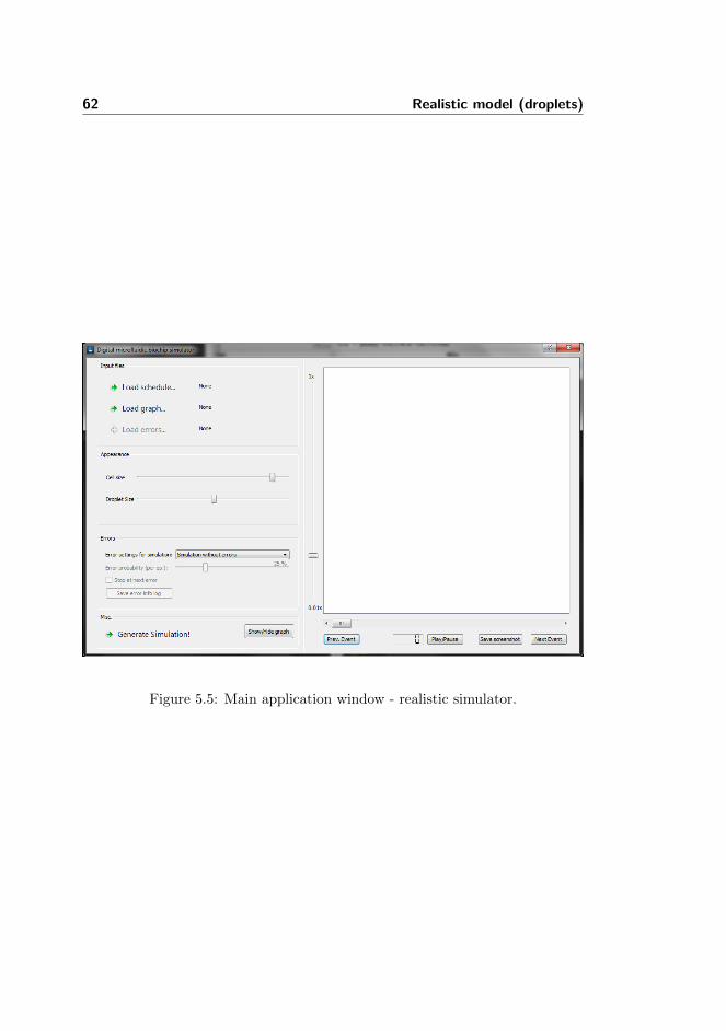
62 Realistic model (droplets)
Figure 5.5: Main application window - realistic simulator.

Chapter 6
Faults simulation
Apart from the regular, error free simulation, there is also a possibility to intro-duce volume errors to the simulation. This feature has been designed to offerthree possibilities to the user. Firstly, it is possible to generate random errorsto arbitrary operations. Secondly, user can choose to load an error file includingsuch errors, i.e. ones that apply to specific operations and to them only. Finallyit is possible to set error limit values for intrinsic operation errors, which wouldthen propagate through the operations.
6.1 Erroneous state of the operation
Both in the simplified simulator and in the realistic simulator it is importantto somehow define the erroneous state of the operation. This is one of thereasons why custom Module and Droplet classes have been created. In both ofthem two variables have been added - boolean isCorrupted and errorLevel
(numerical). The first one simply indicates if the operation is erroroneous,whereas the second one determines the actual value of this error (in relationto 1 in the simplified simulator and to the default droplet size in the realisticone). This means that actual generation of an error can be performed by simplychanging the mentioned flag to True and setting some error value.

64 Faults simulation
6.2 Input files
There is only one error file type for the simulation, and it covers both intrinsicand “per operation” errors. The main element is errors and its attribute type
determines what kind of errors will be taken into account by the simulator (ifthe user wants to run the simulation with preset errors) - “i” for intrinsic errorsand “o” for “per operation” errors. Details on how to prepare a correct filewith errors can be found in section 8.4.5.
Intrinsic errors are determined in a single element intrinsic errors, with thefollowing attributes setting the error limit/threshold values:
� edis - error threshold value for dispensing operation,
� edlt - error threshold value for dilution operation,
� emix - error threshold value for mixing operation,
� etrans - error threshold value for transporting operation,
� esplit - error threshold value for split operation operation
Last two are currently not used by the simulator, but since they are a part of thewhole theory behind the intrinsic errors (see section 1.2.4) I decided to includethem. Future improvements may include incorporation of transport and splitoperations, so those two limit values may prove useful. Please also note that ifany of those limits is set to 0 it is treated as if there was no error.
“Per operation” errors are determined in operation elements, one for each error,and each of this elements have two attributes:- opNumber - number of operation affected by the error - opError - thresholdvalue for the specified error
XML schema for the error input file is presented in figure 6.1, and an exampleof a correct input file with errors is given in appendix D.
Please note that it is impossible to load a file with intrinsic errors (error type “i”)without loading a graph (reasons for this will be given in sections below). Anattempt to do so will result in a warning from the program. It should be possible- from the theoretical point of view - to load a list of “per operation” errors (errortype “o”) as they do not require a graph to work correctly. However such anoption has been disabled to minimize the number of checks, and subsequently -a number of mistake opportunities.

6.3 Simulators’ extensions 65
<xsd : schema attributeFormDefault=”unqualified ” elementFormDefault=”←↩qualified ” ve r s i on =”1.0” xmlns : xsd=”http : // www . w3 . org /2001/←↩XMLSchema”>
<xsd : element name=”errors ” type=”errorsType ” /><xsd : complexType name=”errorsType”>
<xsd : sequence><xsd : element minOccurs=”0” maxOccurs=”1” name=”intrinsic_errors ”←↩
type=”intrinsic_errorsType ” /><xsd : element minOccurs=”0” maxOccurs=”unbounded ” name=”operation←↩
” type=”operationType ” /></xsd : sequence><xsd : attribute name=”type” type=”xsd : string ” />
</xsd : complexType><xsd : complexType name=”operationType”>
<xsd : attribute name=”opNumber ” type=”xsd : string ” /><xsd : attribute name=”opError ” type=”xsd : string ” />
</xsd : complexType><xsd : complexType name=”intrinsic_errorsType”>
<xsd : attribute name=”edis ” type=”xsd : string ” /><xsd : attribute name=”edlt ” type=”xsd : string ” /><xsd : attribute name=”emix ” type=”xsd : string ” /><xsd : attribute name=”etrans ” type=”xsd : string ” /><xsd : attribute name=”esplit ” type=”xsd : string ” />
</xsd : complexType></xsd : schema>
Figure 6.1: XSD schema - error input file
6.3 Simulators’ extensions
Several new variables needed to be added to both simulators in order to acco-modate errors feature:
� Edis, Edlt, Emix, Etrans, Edis and Esplit for storing intrinsic errorlimit values for five operation types mentioned in section 1.2.4.
� errBrush for setting a color for an erroneous operation (module ordroplet).
� Flags errorIsOpen (for indication that a correct error input file has beenloaded) and errorOut (indicating that errors happen during the simula-tion and can be saved in a log file).
� inErrorMode for indicating which kind of errors are loaded (intrinsic orsingle operation)
� ERRORMODE - variable indicating whether simulation is running withouterrors (0), with randomly generated errors (1) or with errors loaded froma file(2).

66 Faults simulation
� errors - set containing all the errors that happen throughout the simu-lated schedule.
� Dictionary errTimes - for a faster access to a specific error.
6.4 Error class
Each of the errors is represented as a single Error object. For this purpose anew, really simple class has been created.
A new Error object must be created with the following parameters:
� Operation number,
� Operation super type, to make the error message more informative,
� Time of the error, which is the starting time of an erroneous operation,
� Error value,
A method errorInfo has been provided with this class. It returns the errorinformation as a nicely formatted string (please see detailed error informationin figure 6.2).
Figure 6.2: Error information.
Like in the case of Node, Module and Droplet classes, this is also hashable, withthe hash function returning the operation number.

6.5 Opening the file 67
Figure 6.3: Error - simplified class diagram.
6.5 Opening the file
Loading the error file is quite similar to loading the schedule or graph, and thestep-by-step working principle is as follows:
� Check if the schedule is loaded and if the graph is loaded. If yes, proceed,otherwise display an error message that they are not loaded and stopexecution.
� Choose the file to open. Similarily to the schedule and graph cases, thisis done by opening a standard “Open file...” dialog.
� Validate the file using schema error.xsd. If the validation is successfulproceed, otherwise - display an error message and stop the execution.
� If the validation proved successful - parse the error file. This is only theinitial parsing, whose main purpose is to check if the errors can actuallybe applied to the simulation. This means that the operations in the errorinput file are searched for in the schedule file. If all the operations specifiedin the error file exist in the schedule, True value is returned and the flagindicating the load status of the errors (errorIsOpen) can be set to true,which means that the errors can be generated.This is also the place where the last possible errors in the file can becaught, i.e. errors for operations not present in the schedule. If this is thecase - error message is produced saying that the errors in the file do notmatch the schedule and the function is stopped at this place.

68 Faults simulation
6.6 Generating the errors
If everything is loaded correctly, the simulation with errors can be generated.Depending on the initial settings, i.e. if the errors have been loaded from thefile or are to be generated randomly, three scenarios can happen. Please notethat all the errors - be it random or loaded - are by design generated at thispoint, together with simulation. This means that if the user wants to changesettings for random errors, the simulation needs to be regenerated each time.
6.7 Random errors
Introducing random errors works on an operation-by-operation basis. There aretwo control parameters for these errors - error probability and error limit value.The first one obviously indicates the chance of an error occuring to a givenoperation, the second one sets the limit of this error. As for the distribution ofthe error values - gaussian distribution has been chosen in order to match thetheory behind the intrinsic errors.The simulator is designed in such a way that the user can easily change theerror probability through the program interface, whereas the error limit hasbeen hardcoded as a reasonable value of 0.2 (which is set only once in thesource code so any adjustments are trivial).
The functions setting the errors (corruptModule and corruptModule in sim-plified and realistic simulator respectively) do the following things:
� Determine if the error should occur or not. This is done by generic Pythonrandom generator. In this case randint has been used to generate arandom integer between 1 and 100 (randint has been chosen to ensureuniform distribution of the results). Subsequently this number is comparedto the error probability set by the user. If it is smaller, the operation canbe “corrupted”, otherwise nothing happens.
� Timestamp for the error is created in order to stop the simulation there(if needed). This is set as exactly one frame after the operation starts, sothe error is displayed when the visual representation of the operation (beit a module or a droplet) is already drawn.
� Error variables are updated, which include the flag indicating that theoperation started with an error and the value of this error. The value - asmentioned before - is calculated using gaussian distribution.

6.8 User specified single operation errors 69
� In case of the realistic simulator - droplet size is adjusted accordingly andits color is altered to indicate an error.
� Errors are stored in a set for future use. A custom Error object has beencreated and it includes information about error value, the operation thatis erroneous and the time of the error.
6.8 User specified single operation errors
If user chooses to introduce specific errors to the schedule, the process looksonly slightly different. First of all, error input file is parsed in order to checkthe error mode. If one wishes to visualize specific errors, the type attribute hasto be set to “o”. Only then the simulator can introduce the errors specified inthe file.Then, each operation element is read in, or - to be precise - its opNumber at-tribute. Then a droplet (or module) is looked up in the droplets (modules) set.Finally, program executes the same function that is used in case of random er-rors, but with probability equal to 100% and the error limit taken from attributeopError. The exact error value is again calculated using gaussian distribution.All the remaining actions are exactly the same as in the previous case.
6.9 User specified intrinsic errors
In case of intrinsic errors the situation is more complicated. First of all - theseerrors require information from the graph, as they propagate from operation tooperation and need information about dependencies between the operations.Therefore an iterative approach is needed.Every step below is repeated as long as there are nodes that still have error valuesto be calculated. This is indicated by a boolean flag in each graph node objectwhich is set to True if an error value for this operation node has been calculated.
� If the node has no parents, its value can be determined instantly. It ishowever applicable only to dispensing operation, as it is the only one thatdoes not have a parent operation.
� If the node has parents, check if all of them have the error values alreadycalculated. If yes, error value can be calculated (using formulae presentedin section 1.2.4). Otherwise, proceed to the next iteration.

70 Faults simulation
Having tested numerous input files I deducted that it usually takes at mosttwo iterations to cover all the operations, however I realise that schedules withmore complex dependencies may require more of them.
When the errors are populated, they can be applied to operation modules ordroplets, just like in the previous two cases. Also all the errors are stored in theerror set for future use. Flag indicating that the errors happened (errorOut) isalso set to True.
6.10 Visual error information
It is obvious that all the errors would be useless from the user point of view ifthere was no indication of them at all. Thus the simulator has been designed soas to give the user some control over the error information.First of all, the full error information can be displayed only if the simulationis running automatically, not when the user is skipping through the frames inpause mode. This is simply a matter of convenience resulting from a number oftests using different settings. Errors popping up when the user simply wants toskip through frames proved highly annoying.Taking this into account, timerEvent in both simulators has been upgraded tocheck for errors. It is worth mentioning at this point that it has two levels of“error tolerance”, as indicated by the variable RUNNINGSTATUS. If it is set to 0,the simulation runs smoothly and no information about errors is provided. If itis set to 1, the simulation pauses when the next error occurs.Therefore, if the simulation is set to stop at the next error, after the error oc-cured, information about it is presented to the user. At this point programchecks the error set for all errors that occur at this point. As an Error classprovides a nicely formatted error information message, the program simply col-lects all this information and provides it to the user.When an error occurs, user can see the detailed error information, as the errorwindow is constructed as a generic informational window with “See details...”option. At this point he is required to choose one of three options:
� Break the execution of the simulation and choose a load a new schedule(e.g. one that should exclude the possibility of an error),
� Proceed with the simulation and stop at the next error,
� Proceed with the simulation and ignore the remaining errors (this corre-sponds to setting the RUNNINGSTATUS variable to 0).

6.10 Visual error information 71
However if the user chooses to ignore the remaining errors, he is - at anytime - still able to set up a breakpoint at the next error (i.e. change theRUNNINGSTATUS back to 1) by checking the box “stop at next error”.
The window shown when an error is encountered has been shown in figure 6.2.Below a simulation screenshot with erroneous droplets is presented (fig. 6.4).Please note the different (erroneous) droplet volumes. Also their color has beenchanged (in this case to white) to highlight the error’s occurence.
Figure 6.4: Errors in the realistic simulator.

72 Faults simulation
Similar principles apply to modules, though only their colors are changed (notsizes), see fig. 6.5. In this case only one operation has been affected by an error(operation 6 - mixing).
Figure 6.5: Errors in the simplified simulator.

6.11 Error log 73
6.11 Error log
The last part of handling the errors is the possibility of saving an error log file.This is the main reason for collecting all the errors in a set, because at this pointthe program simply collects error information from all the Error objects storedthere and writes a nicely formatted log text file including all the errors happen.As it was mentioned before, all the errors are generated when “Generate sim-ulation...” button is pressed, therefore the log will include all the errors thathappen during the simulation, no matter at which point it is saved. An exampleof such an error log is presented below.
Operation : 0 , time : 0 , value : −0.0519335266718Operation : 1 , time : 0 , value : −0.0246056254272Operation : 2 , time : 24 , value : 0 .00492378408244Operation : 4 , time : 0 , value : 0 .0360331199652Operation : 5 , time : 40 , value : 0 .00328209011747Operation : 6 , time : 75 , value : −0.00288384829239Operation : 7 , time : 103 , value : −0.000282241908359Operation : 11 , time : 81 , value : −0.0144442574028Operation : 12 , time : 117 , value : −0.0973032945061Operation : 13 , time : 117 , value : −0.085529728241Operation : 14 , time : 131 , value : 0 .00838975598521Operation : 19 , time : 178 , value : −0.00285280263556Operation : 20 , time : 204 , value : 0 .000733058088836Operation : 60 , time : 573 , value : −0.0337992019842Operation : 61 , time : 682 , value : −1.36601323355e−05Operation : 62 , time : 682 , value : −6.32224878443e−05Operation : 63 , time : 658 , value : −0.00540860333446Operation : 67 , time : 799 , value : 0 .00109372606404Operation : 68 , time : 758 , value : 0 .0724340326479Operation : 69 , time : 756 , value : −0.00501630162506Operation : 85 , time : 69 , value : 0 .0245918891858Operation : 86 , time : 21 , value : −0.0258961905818Operation : 90 , time : 244 , value : −0.000685358467117Operation : 91 , time : 207 , value : −0.0323326526876Operation : 95 , time : 265 , value : −0.0339657903008Operation : 96 , time : 562 , value : −0.00105070150828Operation : 97 , time : 492 , value : −0.0769251038657
Figure 6.6: Error log

74 Faults simulation

Chapter 7
Program features
This chapter summarizes all the features of both simulators (together with er-rors). For a bigger readability level the features are grouped by type. Note thatonly simple explanations are given here as the whole design has been explainedin previous sections.Since most of the features are the same for both the simplified and the realisticsimulator, one list covers them both, as it is unnecessary to repeat them twice.
Figure 7.1: File loading buttons.
File loading - three buttons are responsible for loading schedule file, graph fileand error file (the last one is disabled unless “Simulation with pre-set errors(from file)” option is chosen in the combo box in error settings.

76 Program features
Figure 7.2: Appearance settings.
Appearance settings. User can set the size of the biochip cell and either modulesize (in simplified simulator) or the default droplet size (in realistic simulator).
Figure 7.3: Error (faults) settings.
Error settings. Following features are connected to this part:
� Choosing the error mode. Combo box provides options for error-free sim-ulation, simulation with randomly generated errors or with user-specifiederrors. It is up to the user whether this errors are intrinsic or only forsingle operations.
� For a simulation with random errors - setting the probability of an error.
� If simulation is running - setting (or unsetting) a break point at the nexterror, if the check box is checked, the simulation will stop when the nexterror happens.
� Saving error log - if there are any errors happening during simulation, itis possible to save them all into a log file.
Misc. settings. Currently these include only the simulation generation andsetting the visibility of the graph window.
Playback features.

77
Figure 7.4: Misc. settings.
Figure 7.5: Playback settings.
� Playing/Pausing the simulation.
� Moving along the simulation timeline. Clicking the slider’s arrows willmove the simulation 1 step backwards/forwards. Clicking on the slider’sbackground next to the slider will move it 10 steps back/forth.
� Jumping to the previous/next event. Clicking any of those buttons willmove the user to the nearest time when an operation finishes or starts.

78 Program features
� LCD-like display shows the current timeframe.
� “Save screenshot” button exports current simulation frame to a PNG file.This is done simply by using a painter that redraws current scene to anexternal file.
� Changing simulation speed. A vertical slider left to the simulation viewadjusts the simulation speed between 1 step per second and 1 step per 20ms (lowest “safe” time resolution). This option is available only in therealistic simulator.
Features that can be adjusted in source code only.
� Default colors for operations.
� The names for acceptable operations (and colors for these operations)
� Defined types of detectors.

Chapter 8
Instructions of Use
8.1 Requirements
Before it is possible to run the simulator, installation of two things is mandatory:
1. Python environment. Version 3.0 or higher is required as the simulatorhas been developed in Python 3 which is not compatible backward. Forthe optimal performence version 3.1.x is suggested. It can be downloadedat http://www.python.org, where a number of options are available, in-cluding installer for Microsoft Windows and Apple MacOS X (versions10.3+).
2. PyQt4. PyQt4 is required as well as it has been the environment inwhich the graphic interface has been developed. If you are running Mi-crosoft Windows operating system, the installation can be greatly sim-plified by simply using the binary package available at http://www.
riverbankcomputing.co.uk/software/pyqt/download. For PyQt4 in-stallation instructions for other operating systems please refer to the sub-section below.

80 Instructions of Use
8.1.1 Required Linux packages
The best way is to check which packages cover all the features installed by thebinary installer for Windows, i.e.:
� PyQt
� Qt (with database support for MySQL, PostgreSQL, SQLite3 and ODBC)
� Qt Designer
� Qt Linguist
� Qt Assistant
� pyuic4
� pylupdate4
� lrelease
� pyrcc4
� QScintilla
Plus obviously Python itself, as well as SIP (tool generating C++ interface codefor Python). Usually it should be enough if Python, PyQt and Qt packages areinstalled.
If you are running Arch, any Ubuntu mutation or Gentoo, the required packagesare:
� Arch - python3, pyqt, qt and qscintilla ttogether with all the depen-dencies,
� Ubuntu - python-qt4, qt4-dev-tools, python-qt4-dev andpyqt4-dev-tools together with all dependencies + obviously thePython package,
� Gentoo - Python, PyQt and QScintilla packages.
Please make sure that Python is in version at least 3.0 (3.1 preferred, PyQt andQt are at least 4.0 (4.4 preferred). The version of QScintilla used is 2.2.

8.2 Incompatibility issues 81
8.1.2 Manual PyQt4 installation
If you are running an operating system different from Microsoft Windows - oryou are for any reason unable to use the binary installers - you have to performthe following actions:
1. Install Python3, most Linux distributions have Python available on theirdefault package lists. If not - source code can be downloaded from http:
//python.org/download/.
2. Install SIP. This is a tool that generates C++ interface code for Pythonand is absolutely necessary, as Qt is designed for C++. Most of the Linuxdistributions usually have SIP available in their package managers (versionnumber is not a very important issue, though at least 4.0 is required andthere is no guarantee that the program will work with lower versions).If by any chance SIP package is not available in the package manageror you are running MacOS X or another system different from Win-dows/Linux you have to download and install SIP manually. SIP can bedownloaded at http://www.riverbankcomputing.com/software/sip/
download and the detailed installation tutorial is available at http://www.riverbankcomputing.co.uk/static/Docs/sip4/installation.html
3. Install PyQt4. Again, it should be available in most package man-agers if you are using any major Linux distribution. If not, orif you are using another operating system, please download PyQt4source code from http://www.riverbankcomputing.co.uk/software/
pyqt/download and follow the detailed installation instructions avail-able at: http://www.riverbankcomputing.co.uk/static/Docs/PyQt4/pyqt4ref.html#installing-pyqt.
8.2 Incompatibility issues
Since it is a GUI-based appliation, an operating system with a graphical userinterface is obviously required. To minimize the incompatibility chances it uti-lizes as few interface objects as possible, all of which are considered standard.However it is required that GUI of the operating system includes the followingobjects:
� Window elements - buttons, radio buttons, sliders, checkboxes, combo listsetc.,

82 Instructions of Use
� Message box windows,
� File open and save dialogs,
� Colour pick windows,
All of these features are currently available on the most popular platforms, i.e.Windows, MacOS X and most of the Linux variations. Users of less popularLinux configurations may expect difficulties, depending on the interface used.There was also a known problem of Qt message boxes not displaying the windowtitle on MacOS X, however it is unknown if this problem has been solved or not.It is only a cosmetic issue though.
8.3 Files
The files included are:
� classes.py - custom classes written especially for this simulator,
� uiDroplet.py - user interface for the realistic simulator, compiled fromXML file produced by Qt Designer,
� uiModule.py - user interface for the simplified simulator, compiled fromXML file produced by Qt Designer,
� simDroplet.py - realistic simulator - application file,
� simModule.py - simplified simulator - application file,
� graph.xsd - schema for the graph input file,
� schedModule.xsd - schema for the schedule input file for the simplifiedsimulator,
� schedDroplet.xsd - schema for the schedule input file for the realisticsimulator,
� trnSchedModule.py - converter for the schedule files for simplified simu-lator,
� trnSchedDroplet.py - converter for the schedule files for realistic simu-lator,
� trnGraph.py - converter for the graph files

8.4 Instructions of use 83
8.4 Instructions of use
8.4.1 Simulator window
Both simulators’ windows are very similar. For detailed description of windowcontents and their actions, please refer to section 7.
8.4.2 Preparing the simulation
After choosing which simulator to run - simplified (simModule.py) or realis-tic (simDroplet.py) user should follow these steps (it is assumed that all theneeded input files are already prepared):
1. Choose error mode for the simulation, or leave defaults if a simulationwithout any errors is desired,
2. Load the schedule file.
3. Load the graph file (optional).
4. Load the errors file (optional). This option is enabled only if simulationwith user-set errors has been chosen in step one.
5. Adjust the simulation appearance and parameters (optional).
6. Generate the simulation.
Once the simulation is generated, user has the control over the running of thesimulation.
8.4.3 Running the simulation - basics.
If there were no errors during the simulation, initial frame (at time 0) appearson the right side of the window. Playback controls are present directly belowthe simulation window. In case of the realistic simulation there is also anotherslider on the left side of the simulation view.Now the user has following options available:

84 Instructions of Use
1. Play/pause the simulation. Clicking this button will change the runningstatus of the simulation instantly.
2. Go to an arbitrary point in simulation. Arrows can be used for fine pre-cision of 1 timestamp (centisecond). Clicking on the background of theslider next to the slider skips 10 frames (both ways). Option availableboth during pause and play.
3. Go to the next event (either the nearest start or the nearest end of anoperation). Option available both during pause and play.
4. Go to the previous event (either the nearest start or the nearest end of anoperation). Option available both during pause and play.
5. Change the speed of the simulation. Speed can be changed anywherebetween 0.5x and 0.01x.
6. Export current frame to a PNG file. This will open up a “Save file...”dialog where the destination file can be specified.
8.4.4 Adding the graph
Adding the graph to the simulation is easy. First of all, once the schedule isloaded, please press the “Load graph...” button and choose a valid file (if thefile is by any chance wrong a message will be displayed). Please note thatgraph must be loaded after the schedule and before pressing the “Generatesimulation...” button. Once it is loaded and the simulation is generated thegraph can be toggled on and off by pressing the “show/hide graph” button.
8.4.5 Introducing the errors
Before any errors can be loaded, two conditions must be met:
� Error mode must be set to user-input (last option in the combo box)
� File with errors must be properly prepared.
An example of a well prepared file can be found in appendix ??. Three thingsare essential in this file - error types and well structured input for any of thosetypes.First of all - it is absolutely necessary to indicate the type of errors that are

8.5 Additional tools 85
loaded. This is done by setting the value of type attribute to either “i”(forintrinsic errors) or “o” (for errors applied to single operations). In the first case,values of all five intrinsic error limits must be set (if there’s no error limit value,just enter 0. Note that these are accepted as strings, thus quotations mark arerequired. Entering non-numerical values will result in program malfunction.For single operation errors an element operation must be specified with at-tribute values describing the operation number and the error limit value.In case of any problems please use the template file provided with the programor look at an example in the appendices.
8.4.6 Defining and modifying the operations
The simulator can be easily extended with new operations, though this has tobe performed by editing source code. In both cases the changes required arethe same. To add new operations, please find a line stating:self.brushes = {}Underneath there are definitions of all the operations, for example:self.brushes["opt"] = QColor(255,128,0,127)
To add a new operation, simple copy such a line and change the string in thesquare brackets to the name of the new operation (it is necessary that it isthe same as the operation type within the schedule). Right hand side of thisassignment simply specifies the color associated with this operation, in theform of R,G,B,Alpha.
In the case of realistic simulator, there is a possibility of specifying customdetector types. This is done in the exact same way as adding new operations,but the dictionary used for this purpose is named detBrushes and is placeddirectly below the previous one.
8.5 Additional tools
For the purpose of this project three additional, small tools have been de-veloped. These tools are used to convert plain-text input files I have beenprovided with into XML files compatible with simulator. The reason for notusing the provided files as an input was to make the simulator more independent.
The three tools are XML converters for:

86 Instructions of Use
� schedule file for the simplified simulator,
� schedule file for the realistic simulator,
� graph file,
Their working principles are really simple. They read in the text input file, gothrough it line by line, parse the line word by word, and write the result outto an XML writer. At the end, the whole XML document is written out to adestination file on the disk.
As far as the user interface goes - there is basically none. Upon execution, useris presented with a standard file open dialog and then the input file is chosen.Then the whole conversion process is performed (without any visible indicationapart from the default output to the system console) and - when finished -another window pops up, this time to choose the destination file for saving.
Examples of plain-text input files are presented in the three figures below.
8 opt 3 3 (0 , 6 ) 780 37809 opt 3 3 (4 , 6 ) 660 36606 mix 4 6 (0 , 6 ) 490 7805 mix 3 6 (4 , 6 ) 200 6602 mix 4 6 (0 , 6 ) 200 4907 disR 0 0 (−1,−1) 290 4900 disS 0 0 (−1,−1) 0 2001 disR 0 0 (−1,−1) 0 2003 disR 0 0 (−1,−1) 0 2004 disB 0 0 (−1,−1) 0 200
Figure 8.1: Schedule for simplified simulator

8.5 Additional tools 87
2 opt opt 177 207 [ ( 2 ,3 ) , (2 ,3 ) , (2 ,3 ) , (2 ,3 ) , (2 ,3 ) , (2 ,3 ) , (2 ←↩, 3 ) , (2 ,3 ) , (2 ,3 ) , (2 ,3 ) , (2 ,3 ) , (2 ,3 ) , (2 ,3 ) , (2 ,3 ) , (2 ←↩, 3 ) , (2 ,3 ) , (2 ,3 ) , (2 ,3 ) , (2 ,3 ) , (2 ,3 ) , (2 ,3 ) , (2 ,3 ) , (2 ←↩, 3 ) , (2 ,3 ) , (2 ,3 ) , (2 ,3 ) , (2 ,3 ) , (2 ,3 ) , (2 ,3 ) , (2 ,3 ) , (2 ←↩, 3 ) ]
9 mix mix 131 177 [ ( 4 ,2 ) , (5 ,2 ) , (5 ,1 ) , (6 ,1 ) , (6 ,0 ) , (5 ,0 ) , (5 ←↩, 1 ) , (4 ,1 ) , (4 ,2 ) , (4 ,3 ) , (4 ,4 ) , (4 ,5 ) , (4 ,6 ) , (4 ,6 ) , (4 ←↩, 5 ) , (4 ,4 ) , (4 ,3 ) , (4 ,2 ) , (4 ,1 ) , (4 ,0 ) , (3 ,0 ) , (3 ,1 ) , (4 ←↩, 1 ) , (4 ,0 ) , (4 ,0 ) , (5 ,0 ) , (5 ,1 ) , (5 ,2 ) , (5 ,3 ) , (4 ,3 ) , (3 ←↩, 3 ) , (3 ,2 ) , (3 ,1 ) , (3 ,0 ) , (4 ,0 ) , (4 ,1 ) , (5 ,1 ) , (5 ,0 ) , (4 ←↩, 0 ) , (4 ,0 ) , (3 ,0 ) , (3 ,0 ) , (2 ,0 ) , (2 ,1 ) , (2 ,2 ) , (2 ,2 ) , (2 ←↩, 3 ) ]
8 mix mix 127 169 [ ( 2 ,2 ) , (1 ,2 ) , (1 ,3 ) , (1 ,4 ) , (1 ,5 ) , (0 ,5 ) , (0 ←↩, 5 ) , (0 ,4 ) , (0 ,4 ) , (0 ,3 ) , (0 ,2 ) , (1 ,2 ) , (1 ,1 ) , (1 ,0 ) , (1 ←↩, 0 ) , (0 ,0 ) , (0 ,1 ) , (0 ,2 ) , (0 ,3 ) , (0 ,4 ) , (0 ,5 ) , (1 ,5 ) , (2 ←↩, 5 ) , (3 ,5 ) , (4 ,5 ) , (4 ,4 ) , (4 ,3 ) , (3 ,3 ) , (2 ,3 ) , (1 ,3 ) , (0 ←↩, 3 ) , (0 ,4 ) , (0 ,4 ) , (1 ,4 ) , (1 ,3 ) , (0 ,3 ) , (0 ,4 ) , (0 ,4 ) , (0 ←↩, 5 ) , (0 ,6 ) , (0 ,6 ) , (0 ,5 ) , (0 ,4 ) ]
7 dis disR 101 131 [ ( 5 ,−1) , (5 ,−1) , (5 ,−1) , (5 ,−1) , (5 ,−1) , (5 ←↩,−1) , (5 ,−1) , (5 ,−1) , (5 ,−1) , (5 ,−1) , (5 ,−1) , (5 ,−1) , (5 ←↩,−1) , (5 ,−1) , (5 ,−1) , (5 ,−1) , (5 ,−1) , (5 ,−1) , (5 ,−1) , (5 ←↩,−1) , (5 ,0 ) , (5 ,0 ) , (5 ,0 ) , (5 ,0 ) , (4 ,0 ) , (4 ,0 ) , (4 ,1 ) , (4 ←↩, 2 ) , (4 ,2 ) , (4 ,2 ) , (4 ,2 ) ]
. . .
Figure 8.2: Schedule for realistic simulator
0 dis disS1 dis disR2 opt opt3 dis disB4 mix mix5 dlt dlt6 dis disS7 dis disR8 mix mix9 mix mix
ARC a1_0 FROM t1_0 TO t1_4 TYPE 1ARC a1_1 FROM t1_1 TO t1_4 TYPE 1ARC a1_2 FROM t1_4 TO t1_5 TYPE 1ARC a1_3 FROM t1_3 TO t1_5 TYPE 1ARC a1_5 FROM t1_5 TO t1_8 TYPE 1ARC a1_5 FROM t1_6 TO t1_8 TYPE 1ARC a1_5 FROM t1_5 TO t1_9 TYPE 1ARC a1_5 FROM t1_7 TO t1_9 TYPE 1ARC a1_5 FROM t1_9 TO t1_2 TYPE 1
Figure 8.3: Graph file

88 Instructions of Use

Chapter 9
Conclusions
9.1 Summary
The thesis gives an insight into the possibility of using a simulation tool to verifythe synthesis stage of a digital microfluidic biochip. Firstly, the technologybehind the biochip has been covered (Chapter 1). Then, the purpose of thesimulator has been explained (Chapter 2), as well as the extent to which itcovers the issues mentioned in the first chapter. Next four chapters are devotedto the design of the simulator, covering general design principles and overallsolutions (Chapter 3), the detailed design and implementation of a simplified,module level simulator (Chapter 4) and a realistic, droplet level simulator(Chapter 5), as well as errors that apply to the biochip (Chapter 6). Rest ofthe chapters provided a summary of the simulator’s features as well as detailedinstructions of use.
Summing up, the project gave me an insight into the interesting area of mi-crofluidic biochips. It has shown that a simulation tool can greatly contributeto optimalisation of the synthesis process. And even though not all the plannedfeatures made their way to the final version of the project, I am satisfied withthe end result.

90 Conclusions
Apart from all those I also gained a lot of experience in three software develop-ment areas:
� Programming simulation software,
� Working with GUI based applications,
� Using high-level programming environments for practical applications.
9.2 Future Work
Although the project is finished, it is still missing some features that I wouldlike it to have. Absence of some of them is strictly related to a limited time forthe project, but some of them are simply too complex to introduce at this stage.Below, I summarize some ideas that could be implemented in the simulator inthe future.
� Showing droplets’ movement history. It may be useful to have some kindof indication of the route already taken by the droplet. The idea was todisplay a “tail” of a user-defined length (but with some sensible limit) thatwould simply show the last few locations of the droplet. This feature hasnot been included because it is a reasonable challenge to find a way of anefficient drawing of such a tail so it is refreshed for each new frame. Onthe other hand, a simplified version - showing only one, last location - canbe included in the nearest future.
� Increase in the information amount given to the user. Currently user isgiven a reasonable amount of information about what is happening on thechip, but this may be extended further on. For example, a text output (tothe console) indicating which operations are starting or ending. This is afeature that can be easily introduced and it should be available within afew weeks.
� Propagation of droplet size information. Currently only droplets repre-senting operations affected by errors inherit size from their predecessors.It would be a nice idea to implement some kind of an algorithm that wouldpropagate the droplet volume information through the whole droplet’s lifecycle.
� SVG output instead of PNG. SVG graphics are much more suitable forincluding them in papers. Thus a feature that saves the current frame asan SVG file is desired. Though there is a problem - it is easy to output

9.2 Future Work 91
a specified scene to a PNG painter, but PyQt does not offer an easysolution for converting item-based graphics to SVG, and developing sucha tool would simply include a lot of time.
� Nicer graph window. In the cCurrent version of the simulator, graphwindow is extremely simple, with only one issue in mind - that the nodesmust not collide. In more complex cases this results in a graph that is farfrom easily readable. Thus, a nice idea would be to invent a way to drawa graph based on information from the file (nodes and arcs) on a graphicsscene. This - again - is a complex task that would consume quite a largeamount of time.
� “Lifelike” animation. Having all the required data, it is possible to gener-ate the animation that would resemble the actual biochip in more details.One may for example model it using OpenGL and 3D graphics. Since(Py)Qt has a built-in OpenGL support, it is not an impossible task, justa time consuming one. Of course other techniques may be used as well.
Application of these features may make the simulator much more useful andeven more related to the real-life application.

92 Conclusions

Appendix A
Example of a schedule inputfile - simplified simulator
<?xml ve r s i on =”1.0” encoding=”UTF−8”?><schedule xsize=”7” ysize=”7”><operation deviceLength=”3” deviceWidth=”3” endTime=”14016” ←↩
leftBottomCorner=”(0 ,6) ” opNumber=”31” opSuperType=”opt ” ←↩startTime=”11016”/>
<operation deviceLength=”3” deviceWidth=”3” endTime=”12005” ←↩leftBottomCorner=”(0 ,3) ” opNumber=”38” opSuperType=”opt ” ←↩startTime=”9005”/>
<operation deviceLength=”3” deviceWidth=”3” endTime=”11319” ←↩leftBottomCorner=”(3 ,6) ” opNumber=”39” opSuperType=”opt ” ←↩startTime=”8319”/>
<operation deviceLength=”4” deviceWidth=”4” endTime=”11016” ←↩leftBottomCorner=”(3 ,3) ” opNumber=”26” opSuperType=”mix ” ←↩startTime=”10021”/>
<operation deviceLength=”4” deviceWidth=”4” endTime=”10021” ←↩leftBottomCorner=”(3 ,3) ” opNumber=”21” opSuperType=”mix ” ←↩startTime=”9026”/>
<operation deviceLength=”0” deviceWidth=”0” endTime=”10021” ←↩leftBottomCorner=”(−1,−1)” opNumber=”27” opSuperType=”disS ” ←↩startTime=”9721”/>
<operation deviceLength=”0” deviceWidth=”0” endTime=”9026” ←↩leftBottomCorner=”(−1,−1)” opNumber=”23” opSuperType=”disS ” ←↩startTime=”8726”/>
<operation deviceLength=”6” deviceWidth=”4” endTime=”9005” ←↩leftBottomCorner=”(0 ,3) ” opNumber=”32” opSuperType=”mix ” ←↩startTime=”8715”/>
<operation deviceLength=”6” deviceWidth=”4” endTime=”8715” ←↩leftBottomCorner=”(0 ,3) ” opNumber=”20” opSuperType=”mix ” ←↩startTime=”8425”/>

94 Example of a schedule input file - simplified simulator
<operation deviceLength=”0” deviceWidth=”0” endTime=”8715” ←↩leftBottomCorner=”(−1,−1)” opNumber=”33” opSuperType=”disR ” ←↩startTime=”8415”/>
<operation deviceLength=”0” deviceWidth=”0” endTime=”8425” ←↩leftBottomCorner=”(−1,−1)” opNumber=”22” opSuperType=”disS ” ←↩startTime=”8125”/>
<operation deviceLength=”4” deviceWidth=”6” endTime=”8319” ←↩leftBottomCorner=”(3 ,6) ” opNumber=”34” opSuperType=”mix ” ←↩startTime=”8029”/>
<operation deviceLength=”4” deviceWidth=”6” endTime=”8029” ←↩leftBottomCorner=”(3 ,6) ” opNumber=”24” opSuperType=”mix ” ←↩startTime=”7739”/>
<operation deviceLength=”0” deviceWidth=”0” endTime=”8029” ←↩leftBottomCorner=”(−1,−1)” opNumber=”35” opSuperType=”disR ” ←↩startTime=”7729”/>
<operation deviceLength=”4” deviceWidth=”6” endTime=”7739” ←↩leftBottomCorner=”(3 ,6) ” opNumber=”15” opSuperType=”mix ” ←↩startTime=”7449”/>
<operation deviceLength=”0” deviceWidth=”0” endTime=”7739” ←↩leftBottomCorner=”(−1,−1)” opNumber=”25” opSuperType=”disR ” ←↩startTime=”7439”/>
<operation deviceLength=”4” deviceWidth=”6” endTime=”7449” ←↩leftBottomCorner=”(3 ,6) ” opNumber=”14” opSuperType=”mix ” ←↩startTime=”7159”/>
<operation deviceLength=”0” deviceWidth=”0” endTime=”7449” ←↩leftBottomCorner=”(−1,−1)” opNumber=”17” opSuperType=”disR ” ←↩startTime=”7149”/>
<operation deviceLength=”4” deviceWidth=”4” endTime=”7159” ←↩leftBottomCorner=”(3 ,3) ” opNumber=”7” opSuperType=”mix ” ←↩startTime=”6164”/>
<operation deviceLength=”0” deviceWidth=”0” endTime=”7159” ←↩leftBottomCorner=”(−1,−1)” opNumber=”16” opSuperType=”disR ” ←↩startTime=”6859”/>
<operation deviceLength=”6” deviceWidth=”3” endTime=”6324” ←↩leftBottomCorner=”(0 ,6) ” opNumber=”12” opSuperType=”dlt ” ←↩startTime=”5864”/>
<operation deviceLength=”3” deviceWidth=”3” endTime=”9026” ←↩leftBottomCorner=”(0 ,6) ” opNumber=”12” opSuperType=”store ” ←↩startTime=”6324”/>
<operation deviceLength=”0” deviceWidth=”0” endTime=”6164” ←↩leftBottomCorner=”(−1,−1)” opNumber=”9” opSuperType=”disB ” ←↩startTime=”5864”/>
<operation deviceLength=”0” deviceWidth=”0” endTime=”5864” ←↩leftBottomCorner=”(−1,−1)” opNumber=”13” opSuperType=”disB ” ←↩startTime=”5564”/>
<operation deviceLength=”3” deviceWidth=”3” endTime=”5795” ←↩leftBottomCorner=”(0 ,6) ” opNumber=”30” opSuperType=”opt ” ←↩startTime=”2795”/>
<operation deviceLength=”6” deviceWidth=”4” endTime=”2795” ←↩leftBottomCorner=”(0 ,6) ” opNumber=”36” opSuperType=”mix ” ←↩startTime=”2505”/>
<operation deviceLength=”6” deviceWidth=”3” endTime=”2505” ←↩leftBottomCorner=”(0 ,6) ” opNumber=”28” opSuperType=”mix ” ←↩startTime=”2045”/>
<operation deviceLength=”0” deviceWidth=”0” endTime=”2505” ←↩leftBottomCorner=”(−1,−1)” opNumber=”37” opSuperType=”disR ” ←↩startTime=”2205”/>
<operation deviceLength=”6” deviceWidth=”4” endTime=”2045” ←↩leftBottomCorner=”(0 ,6) ” opNumber=”18” opSuperType=”mix ” ←↩startTime=”1755”/>
. . .</schedule>

Appendix B
Example of a schedule inputfile - realistic simulator
<?xml ve r s i on =”1.0” encoding=”UTF−8”?><schedule xsize=”10” ysize=”10”><operation endTime=”895” opNumber=”74” opSuperType=”opt ” opType=”←↩
opt ” startTime=”865”>[ ( 2 , 3 ) , ( 2 , 3 ) , ( 2 , 3 ) , ( 2 , 3 ) , ( 2 , 3 ) , ( 2 , 3 ) , ( 2 , 3 ) , ( 2 , 3 ) , ( 2 , 3 ) , ( 2 , 3 ) , ( 2 , 3 )←↩
, ( 2 , 3 ) , ( 2 , 3 ) , ( 2 , 3 ) , ( 2 , 3 ) , ( 2 , 3 ) , ( 2 , 3 ) , ( 2 , 3 ) , ( 2 , 3 ) , ( 2 , 3 ) , ( 2 , 3 )←↩, ( 2 , 3 ) , ( 2 , 3 ) , ( 2 , 3 ) , ( 2 , 3 ) , ( 2 , 3 ) , ( 2 , 3 ) , ( 2 , 3 ) , ( 2 , 3 ) , ( 2 , 3 ) , ( 2 , 3 ) ]
</operation><operation endTime=”887” opNumber=”75” opSuperType=”opt ” opType=”←↩
opt ” startTime=”857”>[ ( 4 , 3 ) , ( 4 , 3 ) , ( 4 , 3 ) , ( 4 , 3 ) , ( 4 , 3 ) , ( 4 , 3 ) , ( 4 , 3 ) , ( 4 , 3 ) , ( 4 , 3 ) , ( 4 , 3 ) , ( 4 , 3 )←↩
, ( 4 , 3 ) , ( 4 , 3 ) , ( 4 , 3 ) , ( 4 , 3 ) , ( 4 , 3 ) , ( 4 , 3 ) , ( 4 , 3 ) , ( 4 , 3 ) , ( 4 , 3 ) , ( 4 , 3 )←↩, ( 4 , 3 ) , ( 4 , 3 ) , ( 4 , 3 ) , ( 4 , 3 ) , ( 4 , 3 ) , ( 4 , 3 ) , ( 4 , 3 ) , ( 4 , 3 ) , ( 4 , 3 ) , ( 4 , 3 ) ]
</operation><operation endTime=”886” opNumber=”73” opSuperType=”opt ” opType=”←↩
opt ” startTime=”856”>[ ( 4 , 5 ) , ( 4 , 5 ) , ( 4 , 5 ) , ( 4 , 5 ) , ( 4 , 5 ) , ( 4 , 5 ) , ( 4 , 5 ) , ( 4 , 5 ) , ( 4 , 5 ) , ( 4 , 5 ) , ( 4 , 5 )←↩
, ( 4 , 5 ) , ( 4 , 5 ) , ( 4 , 5 ) , ( 4 , 5 ) , ( 4 , 5 ) , ( 4 , 5 ) , ( 4 , 5 ) , ( 4 , 5 ) , ( 4 , 5 ) , ( 4 , 5 )←↩, ( 4 , 5 ) , ( 4 , 5 ) , ( 4 , 5 ) , ( 4 , 5 ) , ( 4 , 5 ) , ( 4 , 5 ) , ( 4 , 5 ) , ( 4 , 5 ) , ( 4 , 5 ) , ( 4 , 5 ) ]
</operation><operation endTime=”865” opNumber=”67” opSuperType=”mix ” opType=”←↩
mix ” startTime=”799”>[ ( 1 , 2 ) , ( 2 , 2 ) , ( 2 , 2 ) , ( 3 , 2 ) , ( 3 , 3 ) , ( 3 , 4 ) , ( 3 , 5 ) , ( 2 , 5 ) , ( 1 , 5 ) , ( 0 , 5 ) , ( 0 , 6 )←↩
, ( 1 , 6 ) , ( 1 , 5 ) , ( 0 , 5 ) , ( 0 , 5 ) , ( 1 , 5 ) , ( 2 , 5 ) , ( 2 , 4 ) , ( 2 , 4 ) , ( 2 , 5 ) , ( 2 , 6 )←↩, ( 3 , 6 ) , ( 3 , 7 ) , ( 2 , 7 ) , ( 1 , 7 ) , ( 1 , 8 ) , ( 2 , 8 ) , ( 3 , 8 ) , ( 3 , 7 ) , ( 2 , 7 ) , ( 2 , 6 )←↩, ( 2 , 5 ) , ( 2 , 5 ) , ( 2 , 6 ) , ( 1 , 6 ) , ( 0 , 6 ) , ( 0 , 6 ) , ( 1 , 6 ) , ( 1 , 5 ) , ( 0 , 5 ) , ( 0 , 5 )←↩, ( 0 , 6 ) , ( 0 , 6 ) , ( 1 , 6 ) , ( 2 , 6 ) , ( 2 , 5 ) , ( 3 , 5 ) , ( 3 , 6 ) , ( 2 , 6 ) , ( 2 , 5 ) , ( 3 , 5 )←↩, ( 3 , 6 ) , ( 3 , 7 ) , ( 2 , 7 ) , ( 2 , 8 ) , ( 1 , 8 ) , ( 1 , 9 ) , ( 0 , 9 ) , ( 0 , 8 ) , ( 1 , 8 ) , ( 1 , 7 )←↩, ( 1 , 6 ) , ( 1 , 5 ) , ( 1 , 4 ) , ( 1 , 4 ) , ( 2 , 4 ) , ( 2 , 3 ) ]
</operation>

96 Example of a schedule input file - realistic simulator
<operation endTime=”857” opNumber=”69” opSuperType=”mix ” opType=”←↩mix ” startTime=”756”>
[ ( 4 , 1 ) , ( 3 , 1 ) , ( 2 , 1 ) , ( 2 , 0 ) , ( 3 , 0 ) , ( 2 , 0 ) , ( 1 , 0 ) , ( 0 , 0 ) , ( 0 , 0 ) , ( 1 , 0 ) , ( 0 , 0 )←↩, ( 0 , 0 ) , ( 1 , 0 ) , ( 1 , 0 ) , ( 0 , 0 ) , ( 0 , 1 ) , ( 0 , 1 ) , ( 0 , 1 ) , ( 1 , 1 ) , ( 2 , 1 ) , ( 3 , 1 )←↩, ( 3 , 0 ) , ( 4 , 0 ) , ( 4 , 1 ) , ( 4 , 2 ) , ( 4 , 3 ) , ( 3 , 3 ) , ( 3 , 3 ) , ( 2 , 3 ) , ( 2 , 2 ) , ( 2 , 1 )←↩, ( 2 , 0 ) , ( 3 , 0 ) , ( 4 , 0 ) , ( 4 , 1 ) , ( 3 , 1 ) , ( 2 , 1 ) , ( 2 , 2 ) , ( 2 , 3 ) , ( 2 , 4 ) , ( 2 , 4 )←↩, ( 1 , 4 ) , ( 1 , 5 ) , ( 0 , 5 ) , ( 0 , 4 ) , ( 1 , 4 ) , ( 1 , 5 ) , ( 0 , 5 ) , ( 0 , 5 ) , ( 0 , 4 ) , ( 0 , 3 )←↩, ( 0 , 3 ) , ( 0 , 2 ) , ( 0 , 2 ) , ( 1 , 2 ) , ( 1 , 3 ) , ( 0 , 3 ) , ( 0 , 3 ) , ( 0 , 2 ) , ( 0 , 2 ) , ( 0 , 3 )←↩, ( 0 , 4 ) , ( 0 , 5 ) , ( 0 , 5 ) , ( 0 , 4 ) , ( 0 , 3 ) , ( 0 , 2 ) , ( 0 , 2 ) , ( 0 , 3 ) , ( 0 , 4 ) , ( 0 , 5 )←↩, ( 1 , 5 ) , ( 0 , 5 ) , ( 0 , 4 ) , ( 0 , 4 ) , ( 0 , 3 ) , ( 0 , 2 ) , ( 0 , 3 ) , ( 0 , 3 ) , ( 0 , 4 ) , ( 0 , 3 )←↩, ( 0 , 3 ) , ( 0 , 3 ) , ( 0 , 3 ) , ( 0 , 3 ) , ( 0 , 3 ) , ( 0 , 4 ) , ( 0 , 3 ) , ( 0 , 2 ) , ( 0 , 3 ) , ( 0 , 3 )←↩, ( 0 , 3 ) , ( 0 , 4 ) , ( 0 , 3 ) , ( 0 , 3 ) , ( 0 , 3 ) , ( 1 , 3 ) , ( 2 , 3 ) , ( 2 , 2 ) , ( 3 , 2 ) , ( 4 , 2 )←↩, ( 4 , 3 ) ]
</operation><operation endTime=”856” opNumber=”65” opSuperType=”mix ” opType=”←↩
mix ” startTime=”785”>[ ( 3 , 5 ) , ( 4 , 5 ) , ( 5 , 5 ) , ( 6 , 5 ) , ( 7 , 5 ) , ( 7 , 6 ) , ( 7 , 7 ) , ( 8 , 7 ) , ( 9 , 7 ) , ( 9 , 8 ) , ( 9 , 8 )←↩
, ( 9 , 7 ) , ( 9 , 6 ) , ( 8 , 6 ) , ( 8 , 7 ) , ( 9 , 7 ) , ( 9 , 6 ) , ( 9 , 5 ) , ( 9 , 5 ) , ( 9 , 6 ) , ( 9 , 7 )←↩, ( 8 , 7 ) , ( 7 , 7 ) , ( 6 , 7 ) , ( 6 , 6 ) , ( 5 , 6 ) , ( 5 , 5 ) , ( 5 , 4 ) , ( 4 , 4 ) , ( 4 , 3 ) , ( 5 , 3 )←↩, ( 5 , 2 ) , ( 6 , 2 ) , ( 6 , 1 ) , ( 6 , 0 ) , ( 5 , 0 ) , ( 5 , 0 ) , ( 4 , 0 ) , ( 3 , 0 ) , ( 3 , 1 ) , ( 3 , 1 )←↩, ( 2 , 1 ) , ( 1 , 1 ) , ( 1 , 1 ) , ( 2 , 1 ) , ( 3 , 1 ) , ( 4 , 1 ) , ( 4 , 0 ) , ( 3 , 0 ) , ( 2 , 0 ) , ( 2 , 1 )←↩, ( 1 , 1 ) , ( 0 , 1 ) , ( 0 , 1 ) , ( 1 , 1 ) , ( 2 , 1 ) , ( 3 , 1 ) , ( 2 , 1 ) , ( 2 , 1 ) , ( 2 , 0 ) , ( 3 , 0 )←↩, ( 3 , 0 ) , ( 4 , 0 ) , ( 4 , 1 ) , ( 4 , 2 ) , ( 4 , 3 ) , ( 4 , 3 ) , ( 4 , 3 ) , ( 4 , 4 ) , ( 5 , 4 ) , ( 5 , 5 )←↩, ( 4 , 5 ) ]
</operation><operation endTime=”850” opNumber=”76” opSuperType=”opt ” opType=”←↩
opt ” startTime=”820”>[ ( 2 , 3 ) , ( 2 , 3 ) , ( 2 , 3 ) , ( 2 , 3 ) , ( 2 , 3 ) , ( 2 , 3 ) , ( 2 , 3 ) , ( 2 , 3 ) , ( 2 , 3 ) , ( 2 , 3 ) , ( 2 , 3 )←↩
, ( 2 , 3 ) , ( 2 , 3 ) , ( 2 , 3 ) , ( 2 , 3 ) , ( 2 , 3 ) , ( 2 , 3 ) , ( 2 , 3 ) , ( 2 , 3 ) , ( 2 , 3 ) , ( 2 , 3 )←↩, ( 2 , 3 ) , ( 2 , 3 ) , ( 2 , 3 ) , ( 2 , 3 ) , ( 2 , 3 ) , ( 2 , 3 ) , ( 2 , 3 ) , ( 2 , 3 ) , ( 2 , 3 ) , ( 2 , 3 ) ]
</operation><operation endTime=”820” opNumber=”71” opSuperType=”mix ” opType=”←↩
mix ” startTime=”771”>[ ( 1 , 3 ) , ( 0 , 3 ) , ( 0 , 4 ) , ( 0 , 5 ) , ( 0 , 6 ) , ( 0 , 7 ) , ( 0 , 7 ) , ( 0 , 8 ) , ( 1 , 8 ) , ( 1 , 7 ) , ( 0 , 7 )←↩
, ( 0 , 8 ) , ( 0 , 9 ) , ( 0 , 9 ) , ( 0 , 9 ) , ( 0 , 8 ) , ( 0 , 7 ) , ( 1 , 7 ) , ( 2 , 7 ) , ( 3 , 7 ) , ( 4 , 7 )←↩, ( 5 , 7 ) , ( 5 , 6 ) , ( 5 , 5 ) , ( 6 , 5 ) , ( 7 , 5 ) , ( 7 , 4 ) , ( 7 , 3 ) , ( 7 , 2 ) , ( 6 , 2 ) , ( 6 , 1 )←↩, ( 6 , 0 ) , ( 5 , 0 ) , ( 4 , 0 ) , ( 4 , 0 ) , ( 3 , 0 ) , ( 2 , 0 ) , ( 1 , 0 ) , ( 0 , 0 ) , ( 0 , 0 ) , ( 1 , 0 )←↩, ( 1 , 1 ) , ( 2 , 1 ) , ( 2 , 2 ) , ( 2 , 2 ) , ( 2 , 2 ) , ( 2 , 2 ) , ( 3 , 2 ) , ( 2 , 2 ) , ( 2 , 3 ) ]
</operation><operation endTime=”799” opNumber=”68” opSuperType=”dis ” opType=”←↩
disS ” startTime=”758”>[ (0 ,−1) ,(0 ,−1) ,(0 ,−1) ,(0 ,−1) ,(0 ,−1) ,(0 ,−1) ,(0 ,−1) ,(0 ,−1) ,(0 ,−1)←↩
,(0 ,−1) ,(0 ,−1) ,(0 ,−1) ,(0 ,−1) ,(0 ,−1) ,(0 ,−1) ,(0 ,−1) ,(0 ,−1)←↩,(0 ,−1) ,(0 ,−1) ,(0 ,−1) , ( 0 , 0 ) , ( 0 , 1 ) , ( 0 , 2 ) , ( 1 , 2 ) , ( 1 , 3 ) , ( 0 , 3 )←↩, ( 0 , 4 ) , ( 0 , 3 ) , ( 0 , 2 ) , ( 0 , 2 ) , ( 0 , 2 ) , ( 1 , 2 ) , ( 1 , 3 ) , ( 0 , 3 ) , ( 0 , 2 ) , ( 0 , 3 )←↩, ( 0 , 3 ) , ( 0 , 2 ) , ( 1 , 2 ) , ( 1 , 2 ) , ( 1 , 2 ) , ( 1 , 2 ) ]
</operation><operation endTime=”799” opNumber=”115” opSuperType=”mergeDlt ” ←↩
opType=”mergeDlt ” startTime=”778”>[ ( 8 , 7 ) , ( 8 , 7 ) , ( 7 , 7 ) , ( 7 , 6 ) , ( 8 , 6 ) , ( 8 , 5 ) , ( 8 , 4 ) , ( 7 , 4 ) , ( 7 , 3 ) , ( 6 , 3 ) , ( 5 , 3 )←↩
, ( 4 , 3 ) , ( 4 , 3 ) , ( 5 , 3 ) , ( 5 , 3 ) , ( 4 , 3 ) , ( 5 , 3 ) , ( 4 , 3 ) , ( 4 , 2 ) , ( 3 , 2 ) , ( 2 , 2 )←↩, ( 1 , 2 ) ]
</operation><operation endTime=”785” opNumber=”66” opSuperType=”dis ” opType=”←↩
disR ” startTime=”758”>[ (−1 ,3) ,(−1 ,3) ,(−1 ,3) ,(−1 ,3) ,(−1 ,3) ,(−1 ,3) ,(−1 ,3) ,(−1 ,3) ,(−1 ,3)←↩
,(−1 ,3) ,(−1 ,3) ,(−1 ,3) ,(−1 ,3) ,(−1 ,3) ,(−1 ,3) ,(−1 ,3) ,(−1 ,3)←↩,(−1 ,3) ,(−1 ,3) ,(−1 ,3) , ( 0 , 3 ) , ( 0 , 4 ) , ( 1 , 4 ) , ( 1 , 5 ) , ( 2 , 5 ) , ( 2 , 5 )←↩, ( 2 , 5 ) , ( 3 , 5 ) ]
</operation>. . .
</schedule>

Appendix C
Example of a graph input file
<?xml ve r s i on =”1.0” encoding=”UTF−8”?><graph><node in=”” nodeNum=”0” opSuperType=”dis ” opType=”disS ” out=”2”/><node in=”” nodeNum=”1” opSuperType=”dis ” opType=”disB ” out=”2”/><node in=”0 1” nodeNum=”2” opSuperType=”dlt ” opType=”dlt ” out=”6 ←↩
7”/><node in=”” nodeNum=”3” opSuperType=”dis ” opType=”disR ” out=”5”/><node in=”” nodeNum=”4” opSuperType=”dis ” opType=”disB ” out=”5”/><node in=”3 4” nodeNum=”5” opSuperType=”dlt ” opType=”dlt ” out=”8 ←↩
9”/><node in=”2 10” nodeNum=”6” opSuperType=”mix ” opType=”mix ” out←↩
=”14”/><node in=”2 11” nodeNum=”7” opSuperType=”mix ” opType=”mix ” out←↩
=”16”/><node in=”5 12” nodeNum=”8” opSuperType=”mix ” opType=”mix ” out←↩
=”18”/><node in=”5 13” nodeNum=”9” opSuperType=”mix ” opType=”mix ” out←↩
=”20”/><node in=”” nodeNum=”10” opSuperType=”dis ” opType=”disR ” out=”6”/><node in=”” nodeNum=”11” opSuperType=”dis ” opType=”disS ” out=”7”/><node in=”” nodeNum=”12” opSuperType=”dis ” opType=”disR ” out=”8”/><node in=”” nodeNum=”13” opSuperType=”dis ” opType=”disS ” out=”9”/><node in=”6 15” nodeNum=”14” opSuperType=”dlt ” opType=”dlt ” out←↩
=”22 23”/><node in=”” nodeNum=”15” opSuperType=”dis ” opType=”disB ” out←↩
=”14”/><node in=”7 17” nodeNum=”16” opSuperType=”mix ” opType=”mix ” out←↩
=”26”/><node in=”” nodeNum=”17” opSuperType=”dis ” opType=”disS ” out←↩
=”16”/><node in=”8 19” nodeNum=”18” opSuperType=”dlt ” opType=”dlt ” out←↩
=”28 29”/>

98 Example of a graph input file
<node in=”” nodeNum=”19” opSuperType=”dis ” opType=”disB ” out←↩=”18”/>
<node in=”9 21” nodeNum=”20” opSuperType=”mix ” opType=”mix ” out←↩=”32”/>
<node in=”” nodeNum=”21” opSuperType=”dis ” opType=”disR ” out←↩=”20”/>
<node in=”14 24” nodeNum=”22” opSuperType=”mix ” opType=”mix ” out←↩=”34”/>
<node in=”14 25” nodeNum=”23” opSuperType=”mix ” opType=”mix ” out←↩=”36”/>
<node in=”” nodeNum=”24” opSuperType=”dis ” opType=”disR ” out←↩=”22”/>
<node in=”” nodeNum=”25” opSuperType=”dis ” opType=”disS ” out←↩=”23”/>
<node in=”16 27” nodeNum=”26” opSuperType=”dlt ” opType=”dlt ” out←↩=”38 40”/>
<node in=”” nodeNum=”27” opSuperType=”dis ” opType=”disB ” out←↩=”26”/>
<node in=”18 30” nodeNum=”28” opSuperType=”mix ” opType=”mix ” out←↩=”42”/>
<node in=”18 31” nodeNum=”29” opSuperType=”dlt ” opType=”dlt ” out←↩=”44 46”/>
<node in=”” nodeNum=”30” opSuperType=”dis ” opType=”disS ” out←↩=”28”/>
<node in=”” nodeNum=”31” opSuperType=”dis ” opType=”disB ” out←↩=”29”/>
<node in=”20 33” nodeNum=”32” opSuperType=”mix ” opType=”mix ” out←↩=”48”/>
<node in=”” nodeNum=”33” opSuperType=”dis ” opType=”disR ” out←↩=”32”/>
<node in=”22 35” nodeNum=”34” opSuperType=”mix ” opType=”mix ” out←↩=”77”/>
<node in=”” nodeNum=”35” opSuperType=”dis ” opType=”disS ” out←↩=”34”/>
<node in=”23 37” nodeNum=”36” opSuperType=”mix ” opType=”mix ” out←↩=”78”/>
<node in=”” nodeNum=”37” opSuperType=”dis ” opType=”disR ” out←↩=”36”/>
<node in=”26 39” nodeNum=”38” opSuperType=”dlt ” opType=”dlt ” out←↩=”79”/>
<node in=”” nodeNum=”39” opSuperType=”dis ” opType=”disB ” out←↩=”38”/>
<node in=”26 41” nodeNum=”40” opSuperType=”mix ” opType=”mix ” out←↩=”80”/>
<node in=”” nodeNum=”41” opSuperType=”dis ” opType=”disS ” out←↩=”40”/>
<node in=”28 43” nodeNum=”42” opSuperType=”dlt ” opType=”dlt ” out←↩=”81”/>
<node in=”” nodeNum=”43” opSuperType=”dis ” opType=”disB ” out←↩=”42”/>
<node in=”29 45” nodeNum=”44” opSuperType=”mix ” opType=”mix ” out←↩=”82”/>
<node in=”” nodeNum=”45” opSuperType=”dis ” opType=”disR ” out←↩=”44”/>
<node in=”29 47” nodeNum=”46” opSuperType=”mix ” opType=”mix ” out←↩=”83”/>
<node in=”” nodeNum=”47” opSuperType=”dis ” opType=”disS ” out←↩=”46”/>
<node in=”32 49” nodeNum=”48” opSuperType=”dlt ” opType=”dlt ” out←↩=”84”/>
<node in=”” nodeNum=”49” opSuperType=”dis ” opType=”disB ” out←↩=”48”/>
. . .</graph>

Appendix D
Example of an error input file
<?xml ve r s i on =”1.0” encoding=”UTF−8”?><errors type=”i”>
<intrinsic_errors edis=”0.25” edlt=”0.0” emix=”0.0” etrans=”0.0”←↩esplit=”0.0”/>
<operation opNumber=”1” opError=”0.2”/><operation opNumber=”5” opError=”0.1”/>
</errors>

100 Example of an error input file

Bibliography
[1] Krishnendu Chakrabarty, Fei Su Digital Microfluidic Biochips. Synthesis,testing, and reconfiguration techniques. CRC Press 2007.
[2] Robin Hui Liu, Abraham Phillip Lee Integrated biochips for DNA analysis.Springer 2007.
[3] Zhao, Yang, Xu, Tao, Chakrabarty, Krishnendu Control-Path Design andError Recovery in Digital Microfluidic Lab-on-Chip. Journal of EmergingTechnologies in Computing Systems 2009.
[4] Jan Madsen with Elena Maftei, Paul Pop Mapping biochemical applicationsonto microfluidic-based biochips. MPSoC Symposium August 4, 2009.
[5] Mark Summerfield Programming in Python 3. A Complete Introduction tothe Python Language. Second Edition. Addison-Wesley 2010.
[6] Mark Summerfield Rapid GUI Programming with Python and Qt. TheDefinitive Guide to PyQt Programming. Prentice Hall 2010.