A Stokes drift approximation based on thePhillips spectrum∗

Øyvind Breivik†, Jean-Raymond Bidlot‡

Peter A.E.M. Janssen‡

February 2, 2016

Abstract

A new approximation to the Stokes drift velocity profile based on theexact solution for the Phillips spectrum is explored. The profile is comparedwith the monochromatic profile and the recently proposed exponential in-tegral profile. ERA-Interim spectra and spectra from a wave buoy in thecentral North Sea are used to investigate the behaviour of the profile. It isfound that the new profile has a much stronger gradient near the surfaceand lower normalized deviation from the profile computed from the spec-tra. Based on estimates from two open-ocean locations, an average valuehas been estimated for a key parameter of the profile. Given this param-eter, the profile can be computed from the same two parameters as themonochromatic profile, namely the transport and the surface Stokes driftvelocity.

Keywords: Stokes drift; Wave modelling; Stokes-Coriolis force; Langmuirturbulence parameterization; Trajectory modelling.

∗Final version published in Ocean Modell, 2016, doi:10.1016/j.ocemod.2016.01.005†Corresponding author. E-mail: oyvind.breivik@met.no; ORCID Author ID:

0000-0002-2900-8458. Norwegian Meteorological Institute, Alleg 70, NO-5007 Bergen, Nor-way‡European Centre for Medium-Range Weather Forecasts (ECMWF).

1

arX

iv:1

601.

0809

2v2

[ph

ysic

s.ao

-ph]

1 F

eb 2

016

1 Introduction

The Stokes drift (Stokes, 1847) is defined as the difference between the Eulerianvelocity in a point and the average Lagrangian motion of a particle subjected tothe orbital motion uw of a wave field,

vs =

⟨∫ t

uw dt · ∇uw

⟩. (1)

Here the averaging is over a period appropriate for the frequency of surface waves(Leibovich, 1983). The Stokes drift velocity profile is required for a number of im-portant applications in ocean modelling, such as the computation of trajectoriesof drifting objects, oil and other substances (see McWilliams and Sullivan 2000,Breivik et al. 2012, Rohrs et al. 2012, Rohrs et al. 2015 and references in Breiviket al. 2013). Its magnitude and direction is required for the computation of theStokes-Coriolis force which enters the momentum equation in Eulerian ocean mod-els (Hasselmann 1970, Weber 1983, Jenkins 1987, McWilliams and Restrepo 1999,Janssen et al. 2004, Polton et al. 2005, Janssen 2012, and Breivik et al. 2015),

Du

Dt= − 1

ρw

∇p+ (u + vs)× f z +1

ρw

∂τ

∂z. (2)

Here u is the Eulerian current vector, f the Coriolis frequency, ρw the densityof sea water, vs the Stokes drift velocity vector, z the upward unit vector, p thepressure and τ the stress.

Langmuir circulation, first investigated by Langmuir (1938), manifests itself asconvergence streaks on the sea surface roughly aligned with the wind direction.In a series of papers (Craik and Leibovich 1976, Craik 1977, Leibovich 1977, Lei-bovich 1980) a possible instability mechanism arising from a vortex force vs × ωbetween the Stokes drift and the vorticity of the Eulerian current was proposedto explain the phenomenon (named the second Craik-Leibovich mechanism, CL2,by Faller and Caponi 1978). It is now commonly accepted that CL2 is the maincause of Langmuir circulation in the open ocean (Thorpe, 2004). Langmuir turbu-lence is believed to be important for the formation and depth of the ocean surfaceboundary layer (OSBL) (Li and Garrett 1997 and Flor et al. 2010), and a realisticrepresentation of the phenomenon in ocean models is important (see Axell 2002,Rascle et al. 2006). A common parameterisation of the Langmuir turbulence pro-duction term in the turbulent kinetic energy equation relates it to the shear of theStokes drift profile (Skyllingstad and Denbo 1995, McWilliams et al. 1997, Thorpe2004, Kantha and Clayson 2004, Ardhuin and Jenkins 2006, Grant and Belcher2009 and Belcher et al. 2012),

De

Dt= νmS

2 − νhN2 + νmS · ∂vs

∂z− ∂

∂z(w′e)− 1

ρw

∂

∂z(w′p′)− ε. (3)

2

Here, e represents the turbulent kinetic energy per unit mass; w′e′ and w′p′ arethe turbulent transport and pressure correlation terms (Stull 1988, Kantha andClayson 2000). The shear production and the buoyancy production terms arewell known quantities where S · S = S2 = (∂u/∂z)2, and N2 = −(g/ρw)dρw/dz.Further, νh,m are turbulent diffusion coefficients and ε represents the dissipation ofturbulent kinetic energy. It is the term νmS · ∂vs/∂z, representing the Langmuirturbulence production, that is of interest in this study. It is important to notethat it involves the shear of the Stokes drift. This quantity drops off rapidly withdepth, and clearly any parameterisation of the Langmuir production term willdepend heavily on the form of the Stokes drift velocity profile.

Climatologies of the surface Stokes drift have been presented, either basedon wave model integrations (Rascle et al., 2008; Webb and Fox-Kemper, 2011;Tamura et al., 2012; Rascle and Ardhuin, 2013; Carrasco et al., 2014; Webb andFox-Kemper, 2015) or on assumptions of fully developed sea (McWilliams andRestrepo, 1999). However, the Stokes profile is not so readily available as it isexpensive and impractical to integrate the two-dimensional wave spectrum at ev-ery desired vertical level. It is also numerically challenging to pass the full two-dimensional spectrum for every grid point of interest from a wave model to anocean model. As was discussed by Breivik et al. (2014), hereafter BJB, it has beencommon to replace the full Stokes drift velocity profile by a monochromatic profile[see e.g. Skyllingstad and Denbo (1995), McWilliams and Sullivan (2000), Carnielet al. (2005), Polton et al. (2005), Saetra et al. (2007), and Tamura et al. (2012)].But this will lead to an underestimation of the near-surface shear and an overes-timation of the deep Stokes drift (Ardhuin et al., 2009; Webb and Fox-Kemper,2015). This was partly alleviated by the exponential integral profile proposed byBJB, but it too exhibited too weak shear near the surface.

Here we explore a new approximation to the full Stokes drift velocity profilebased on the assumption that the Phillips spectrum (Phillips, 1958) provides areasonable estimate of the intermediate to high-frequency part of the real spec-trum. The paper is organized as follows. First we present the proposed profile inSec 2. We then investigate its behaviour for a selection of parametric spectra inSec 3 before looking at its performance on two-dimensional wave model spectra inSec 4 for two locations with distinct wave climate, namely the North Atlantic andnear Hawaii. The latter location is swell-dominated whereas the former exhibits amix of swell and wind sea (Reistad et al., 2011; Semedo et al., 2015) typical of theextra-tropics. Finally, in Sec 5 we discuss the results and we present our conclu-sions along with some considerations of the usefulness of the proposed profile forocean modelling and trajectory estimation.

3

2 Approximate Stokes drift velocity profiles

For a directional wave spectrum E(ω, θ) the Stokes drift velocity in deep water isgiven by

vs(z) =2

g

∫ 2π

0

∫ ∞0

ω3ke2kzE(ω, θ) dωdθ, (4)

where θ is the direction in which the wave component is travelling, ω is the circularfrequency and k is the unit vector in the direction of wave propagation. This canbe derived from the expression for a wavenumber spectrum in arbitrary depthfirst presented by Kenyon (1969) by using the deep-water dispersion relation ω2 =gk. For simplicity we will now investigate the Stokes drift profile under the one-dimensional frequency spectrum

F (ω) ≡∫ 2π

0

E(ω, θ)dθ,

for which the Stokes drift speed is written

vs(z) =2

g

∫ ∞0

ω3F (ω)e2kz dω. (5)

From Eq (5) it is clear that at the surface the Stokes drift is proportional to thethird spectral moment [where the n-th spectral moment of the circular frequencyis defined as mn =

∫∞0ωnF (ω) dω],

v0 = 2m3/g. (6)

A new approximation to the Stokes drift profile was proposed by BJB, andnamed the exponential integral profile,

ve = v0e2kez

1− Ckez, (7)

where the constant C = 8 was found to give the closest match. Here, the inversedepth scale ke serves the same purpose as the average wavenumber km used for amonochromatic profile,

vm = v0e2kmz. (8)

The profile (7) was found to be a much better approximation than the monochro-matic profile (8) with a 60% reduction in root-mean-square error reported by BJB,and has been implemented in the Integrated Forecast System (IFS) of the Euro-pean Centre for Medium-Range Weather Forecasts (ECMWF); see Janssen et al.(2013) and Breivik et al. (2015).

4

Here we propose a profile based on the assumption that the Phillips spectrum(Phillips, 1958)

FPhil =

{αg2ω−5, ω > ωp

0, ω ≤ ωp, (9)

yields a reasonable estimate of the part of the spectrum which contributes mostto the Stokes drift velocity near the surface, i.e., the high-frequency waves. Hereωp is the peak frequency. We assume Phillips’ parameter α = 0.0083. The Stokesdrift velocity profile under (9) is

vPhil(z) = 2αg

∫ ∞ωp

ω−2e2ω2z/g dω. (10)

An analytical solution exists for (10), see BJB, Eq (11), which after using thedeep-water dispersion relation can be written as

vPhil(z) =2αg

ωp

[exp (2kpz)−

√−2πkpz erfc

(√−2kpz

)]. (11)

Here erfc is the complementary error function and kp = ω2p/g is the peak wavenum-

ber. From (11) we see that for the Phillips spectrum (10) the surface Stokes driftvelocity is

v0 ≡ vPhil(z = 0) =2αg

ωp

. (12)

For large depths, i.e. as z → −∞, Eq (11) approaches the asymptotic limit [seeBJB, Eqs (14)-15)]

limz→−∞

vPhil = − v0

4kpze2kpz. (13)

This means the exponential integral profile (7) proposed by BJB has too strongdeep flow when fitted to the Phillips spectrum. This could be alleviated by settingthe coefficient C = 4 in Eq (7), but at the expense of increasing the overall root-mean-square (rms) deviation over the water column. Further, although the profile(7) is well suited to modelling the shear at intermediate water depths, its shearnear the surface is too weak. Under the Phillips spectrum (10) the shear is

∂vPhil

∂z= 4α

∫ ∞ωp

e2ω2z/g dω, (14)

for which an analytical expression exists [see Gradshteyn and Ryzhik (2007),Eq (3.321.2)],

∂vPhil

∂z= α

√−2πg

zerfc

(√−2kpz

). (15)

5

Near the surface the shear tends to infinity. This strong shear is not captured byeither the exponential integral profile (7) or the monochromatic profile (8).

Let us now assume that the Phillips spectrum profile (11) is also a reasonableapproximation for Stokes drift velocity profiles under a general spectrum, and thatthe low-frequency part below the peak contributes little to the overall Stokes driftprofile so that it can be ignored. The general profile (5) can be integrated by parts,and for convenience we introduce the quantity

G(ω) =

∫ω3F (ω) dω + C1, (16)

where C1 is a constant of integration. The integral (5) can now be written

vs(z) =2

g

(−G(ωp)e2ω2

pz/g − 4z

g

∫ ∞ωp

ωG(ω)e2ω2z/g dω

). (17)

We note that for the Phillips spectrum (9), the quantity ωG(ω) becomes

ωGPhil(ω) = ω

[∫ ω

ωp

s3FPhil(s) ds+ C1

]= −αg2 + αg2 ω

ωp

+ C1ω, (18)

which is a constant, −αg2, if we set C1 = −αg2/ωp. In this case the solution toEq (17) is Eq (11) as would be expected.

Assume now that in the range ωp < ω < ∞ the quantity ωG(ω) is quite flatalso for an arbitrary spectrum, and that it drops to zero below ωp. Introduce

β = −〈ωG(ω)〉m3ωp

,

where the averaging operator is defined over a range of frequencies, ∆ω, from thepeak frequency to a cutoff frequency, ωc, such that 〈X〉 ≡ ∆ω−1

∫ ωc

ωpX dω. Since

we have assumed β to be constant the ωG(ω) in the second term of Eq (17) canbe factored out and we can approximate Eq (17) by Eq (11),

vs(z) ≈ v0

[e2kpz − β

√−2kpπz erfc

(√−2kpz

)]. (19)

We note that if F is the Phillips spectrum (9) then

〈ωGPhil(ω)〉 = −〈ω5FPhil(ω)〉 = −αg2. (20)

Assuming this to be a reasonable approximation for general spectra we find thatwe can approximate β as follows,

β =2〈ω5F (ω)〉gv0ωp

. (21)

6

Here we have substituted m3 = 2v0/g. The Stokes transport V =∫ 0

−∞ v dz underEq (19) can be found [see A and Gradshteyn and Ryzhik 2007, Eq (6.281.1)] to be

V =v0

2kp

(1− 2β/3). (22)

Provided the transport and the surface Stokes drift are known, as is usually thecase with wave models, we can now use the assumption that the Phillips spectrumis a good representation of the Stokes drift to determine an inverse depth scale kby substituting it for the peak wavenumber kp in Eq (22),

k =v0

2V(1− 2β/3). (23)

Note that we still need to estimate β, which for the Phillips spectrum is exactlyone.

3 Parametric spectra

We now test the profile (19) on a range of other parametric spectra. In each casewe have estimated β by averaging over the range from the peak frequency ωp to acut-off frequency here set at ωc = 10ωp.

Table 1 summarizes the normalized rms (NRMS) error of the Phillips profileapproximation and the previously studied exponential integral profile. The NRMSis defined as the difference between the speed of the approximate profile (mod)and the speed of the full profile, divided by the transport (which is numericallyintegrated from the full profile),

δv = V −1

∫ 0

−H|vmod − v| dz. (24)

Here H is some depth below which the Stokes drift can be considered negligiblysmall.

We first compare the Phillips spectrum against the Phillips approximation.Here, β = 1 and any discrepancy in terms of NRMS is due to roundoff error. Wethen investigate the fit to the Pierson-Moskowitz (PM) spectrum (Pierson andMoskowitz, 1964) for fully developed sea states,

FPM(ω) = αg2ω−5 exp

[−5

4

(ωp

ω

)4]. (25)

As seen in Table 1, the NRMS under the PM spectrum is markedly reduced withthe new profile. The β value is also quite close to unity. This is also the case

7

for the JONSWAP spectrum (Hasselmann et al., 1973), with a peak enhancementfactor γ = 3.3,

FJONSWAP(ω) = FPMγΓ, (26)

where

Γ = exp

[−1

2

(ω/ωp − 1

σ

)2]. (27)

Here σ is a measure of the width of the peak. We have also looked at bimodal,unidirectional spectra by adding a narrow Gaussian spectrum representing 1.5m swell at 0.15 Hz and 0.05 Hz to a JONSWAP and PM wind sea spectrum,respectively. We see in Table 1 that the estimates of β for the combined swell andwind sea spectra are still close to unity. The NRMS difference is markedly higherfor the exponential integral profile proposed by BJB for all spectra, including thebimodal ones.

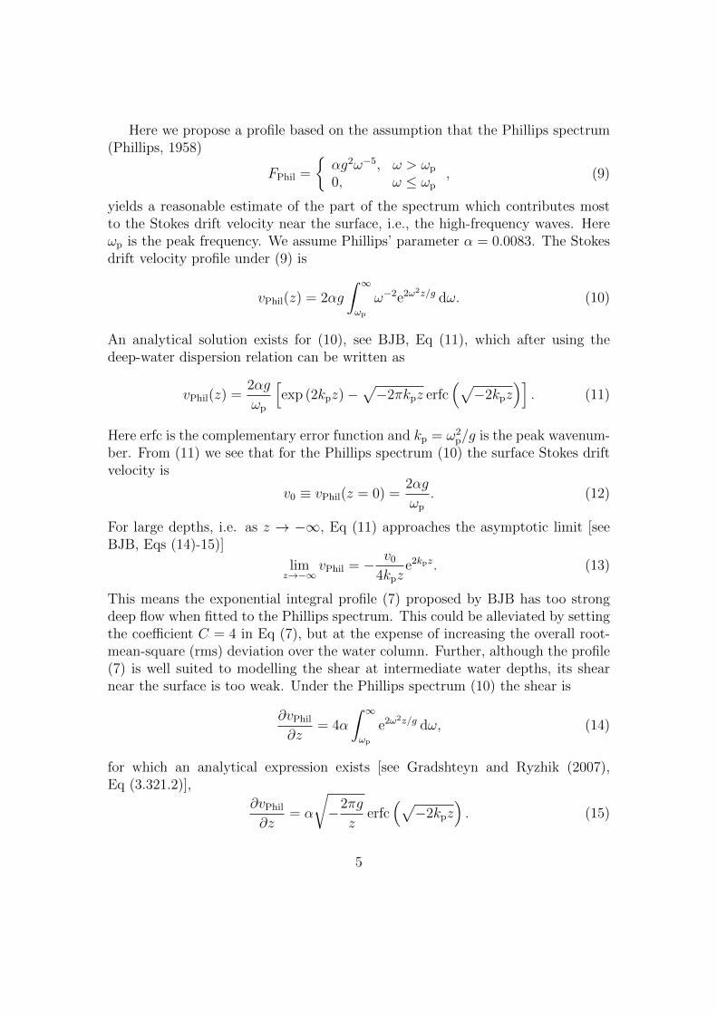
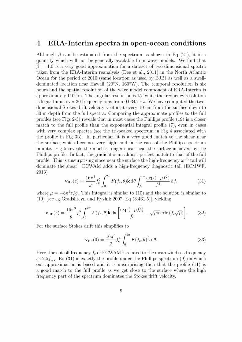
The assumption that the Phillips profile is a good fit to parametric spectra canalso be tested in a more straightforward manner without making any assumptionof the behaviour of the quantity ωG(ω) by simply fitting a Phillips profile (β = 1)to various spectra. In Fig 1 we have fitted the Phillips profile to the surfaceStokes drift v0 and the transport V from parametric spectra and compared theapproximate profile to the full profile. The results show that for the Phillipsspectrum the approximation matches the full profile (to within roundoff error).More interestingly, the Pierson-Moskowitz and the JONSWAP spectra are bothvery well represented by the Phillips approximation (see Fig 1). This simplyconfirms what we found in Table 1. A more challenging case is the Donelan-Hamilton-Hui (DHH) spectrum (Donelan et al., 1985) which has an ω−4 tail,

FDHH(ω) = αg2ω−4ω−1p e−(ωp/ω)4γΓ, (28)

and will consequently behave very differently in the tail. The spectrum is identicalto the JONSWAP spectrum except for substitution of the peak frequency ωp forω and a Jacobian transformation removing the factor 5/4 in the exponential. It isworth noting that the surface Stokes drift under the DHH spectrum is ill-defined(Webb and Fox-Kemper, 2011, 2015), since

vDHH(0) = αg2ω−1p

∫ ∞0

ω−1e−(ωp/ω)4γΓ dω, (29)

which is unbounded because the integrand asymptotes to

limω→∞

ω−1e−(ωp/ω)4γΓ(ω) = ω−1. (30)

Setting a cut-off frequency at 100ωp yields the results shown in Fig 1 for Tp = 10 s.As can be seen the Phillips approximation is not good, but it does in fact representa small improvement compared with the monochromatic and exponential integralapproximations.

8

4 ERA-Interim spectra in open-ocean conditions

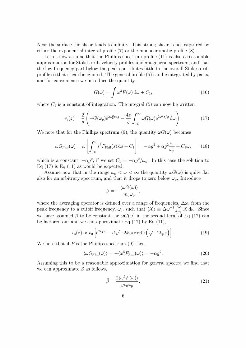
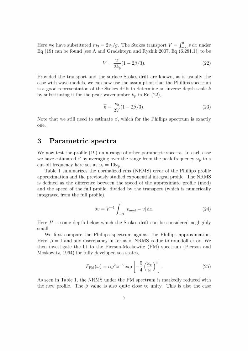
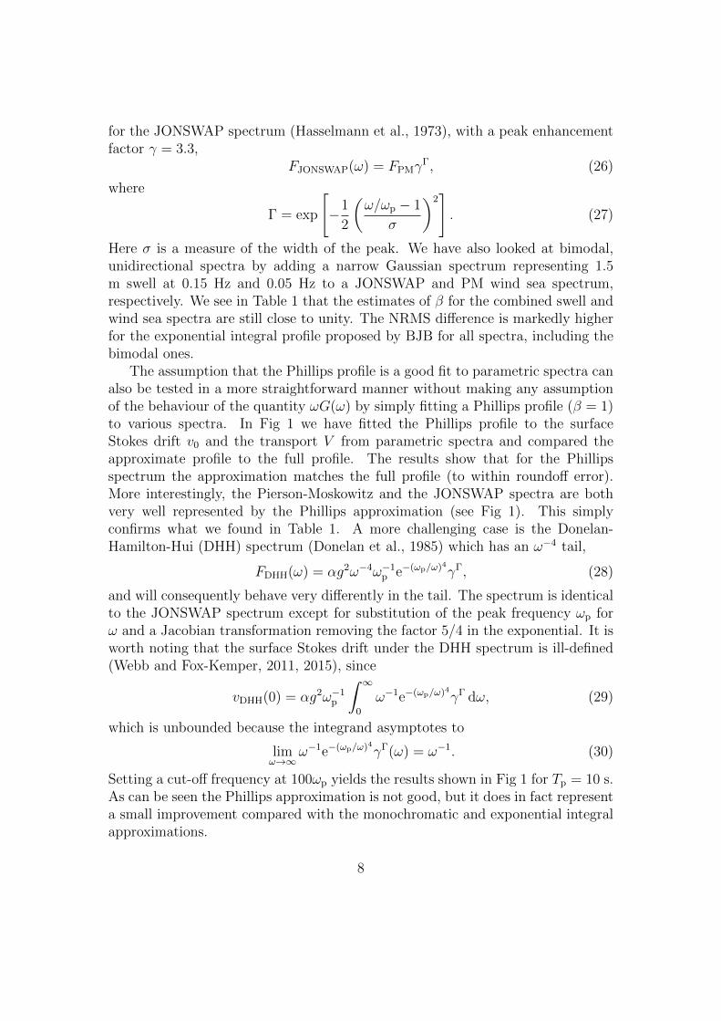
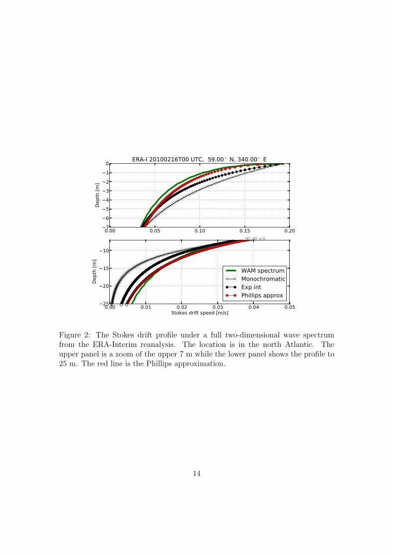
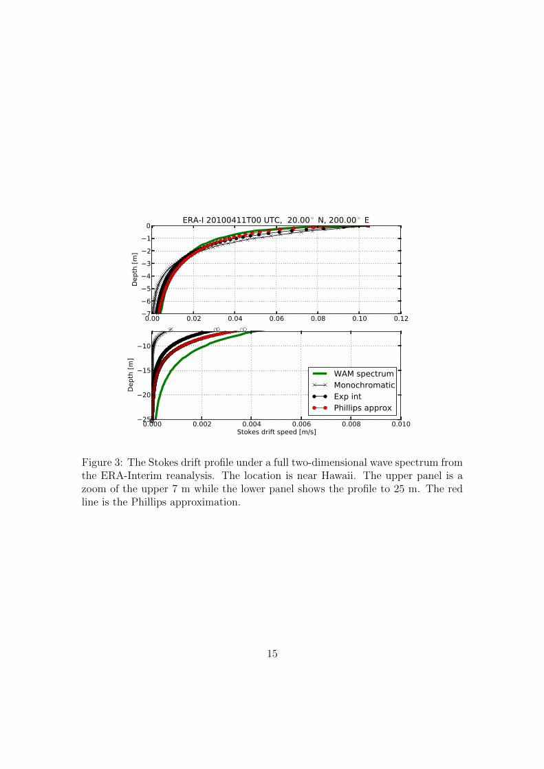
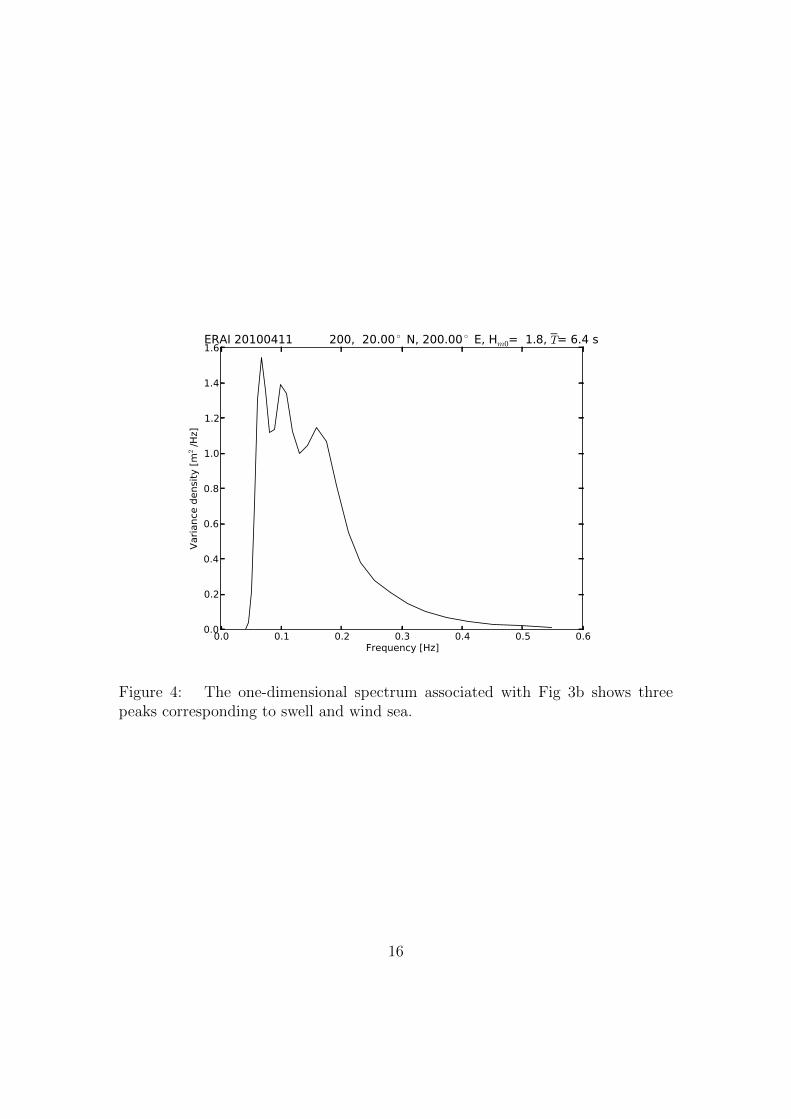
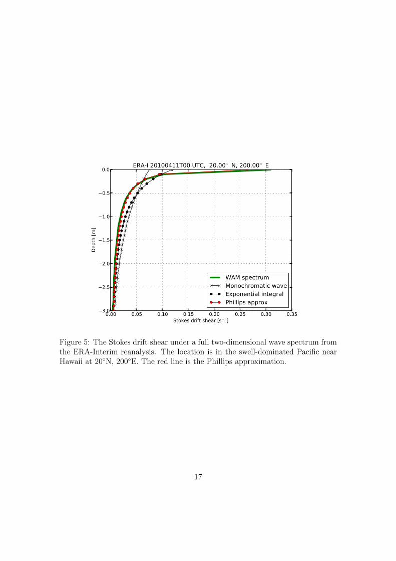
Although β can be estimated from the spectrum as shown in Eq (21), it is aquantity which will not be generally available from wave models. We find thatβ = 1.0 is a very good approximation for a dataset of two-dimensional spectrataken from the ERA-Interim reanalysis (Dee et al., 2011) in the North AtlanticOcean for the period of 2010 (same location as used by BJB) as well as a swell-dominated location near Hawaii (20◦N, 160◦W). The temporal resolution is sixhours and the spatial resolution of the wave model component of ERA-Interim isapproximately 110 km. The angular resolution is 15◦ while the frequency resolutionis logarithmic over 30 frequency bins from 0.0345 Hz. We have computed the two-dimensional Stokes drift velocity vector at every 10 cm from the surface down to30 m depth from the full spectra. Comparing the approximate profiles to the fullprofiles (see Figs 2-3) reveals that in most cases the Phillips profile (19) is a closermatch to the full profile than the exponential integral profile (7), even in caseswith very complex spectra (see the tri-peaked spectrum in Fig 4 associated withthe profile in Fig 3b). In particular, it is a very good match to the shear nearthe surface, which becomes very high, and in the case of the Phillips spectruminfinite. Fig 5 reveals the much stronger shear near the surface achieved by thePhillips profile. In fact, the gradient is an almost perfect match to that of the fullprofile. This is unsurprising since near the surface the high-frequency ω−5 tail willdominate the shear. ECWAM adds a high-frequency diagnostic tail (ECMWF,2013)

vHF(z) =16π3

gf 5

c

∫ 2π

0

F (fc, θ)k dθ

∫ ∞fc

exp (−µf 2)

f 2df, (31)

where µ = −8π2z/g. This integral is similar to (10) and the solution is similar to(19) [see eg Gradshteyn and Ryzhik 2007, Eq (3.461.5)], yielding

vHF(z) =16π3

gf 5

c

∫ 2π

0

F (fc, θ)k dθ

[exp (−µf 2

c )

fc

−√µπ erfc (fc√µ)

]. (32)

For the surface Stokes drift this simplifies to

vHF(0) =16π3

gf 4

c

∫ 2π

0

F (fc, θ)k dθ. (33)

Here, the cut-off frequency fc of ECWAM is related to the mean wind sea frequencyas 2.5fws. Eq (31) is exactly the profile under the Phillips spectrum (9) on whichour approximation is based and it is unsurprising then that the profile (11) isa good match to the full profile as we get close to the surface where the highfrequency part of the spectrum dominates the Stokes drift velocity.

9

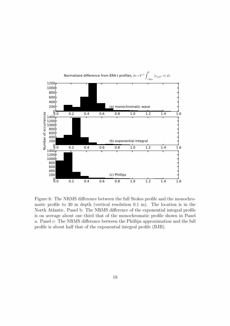
Fig 6 shows that the Phillips profile has an NRMS deviation about half thatof the exponential integral profile for the North Atlantic location. The numbersare quite similar for the Hawaii swell location.

5 Discussion and concluding remarks

Although the exponential integral profile proposed by BJB represents a majorimprovement over the monochromatic profile, it appears clear that the Phillipsprofile (10) is a much better match, especially for representing the shear near thesurface; see Eq (15). Studies of ERA-Interim spectra at two open-ocean locationsnear Hawaii and in the North Atlantic Ocean show that β = 1.0 is a very goodestimate for a wide range of sea states. This allows us to compute the profile fromthe same two parameters as the monochromatic profile, namely the transport andthe surface Stokes drift velocity, and it is thus no more expensive to employ inocean modelling. We have shown here that the profile works remarkably well ina variety of situations, including swell-dominated cases. In C it is shown thatthe profile is also a better match for profiles under measured 2 Hz spectra in thecentral North Sea. This shows that the fit is not dependent on the assumptionof an ω−5 tail since these spectra have no high-frequency diagnostic tail addedto them. The new profile also comes closer to the DHH spectrum which has anω−4 tail, but here the match is naturally quite poor (see Fig 1). We concludethat for applications concerned with the shear of the profile, in particular studiesof Langmuir turbulence, the proposed profile is a much better choice than themonochromatic profile, but it is also clearly a better option than the previouslyproposed exponential integral profile.

The question of how best to represent a full two-dimensional Stokes drift ve-locity profile with a one-dimensional profile was discussed by BJB where it wasargued that using the mean wave direction is better than using the surface Stokesdrift direction since the latter would be heavily weighted toward the direction ofhigh-frequency waves. This still holds true, but it is clear that spreading due tomulti-directional waves affects the Stokes drift [see Webb and Fox-Kemper 2015],and although we model the average profile well, situations with for example op-posing swell and wind waves will greatly modify individual profiles. This will alsoaffect the Langmuir turbulence as parameterised from the Stokes drift velocity pro-file, as demonstrated by McWilliams et al. (2014) for an idealised case of swell andwind waves propagating in different directions. Li et al. (2015) investigated theimpact of wind-wave misalignment and Stokes drift penetration depth on upperocean mixing Southern Ocean warm bias with a coupled wave-atmosphere-oceanearth system model and found that Langmuir turbulence, parameterized using aK-profile parameterization (Large et al., 1994). They found a substantial reduc-

10

tion in the demonstrated that a K-profile parameterization for a coupled systemconsisting of a spectral wave model and the Community Earth System Model.This is impossible to model with a simple parametric profile like the one proposedhere, but a combination of two such parametric profiles, one for the swell and onerepresenting the wind waves is straightforward to implement.

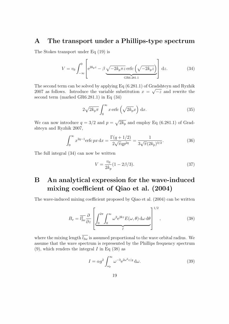
The method presented here to derive an approximate Stokes drift profile basedon the Phillips profile could also be relevant for other wave-related processes.The proposed mixing by non-breaking waves (Babanin, 2006) was implementedin a climate model of intermediate complexity by Babanin et al. (2009) and wascompared against tank measurements by Babanin and Haus (2009). In a similarvein, mixing induced by the wave orbital motion as suggested by Qiao et al. (2004)has been tested for ocean general circulation models (Qiao et al., 2010; Huanget al., 2011; Fan and Griffies, 2014). These suggested mixing parameterizationsbear some semblance to the Langmuir turbulence parameterization in that theyinvolve the shear of an integral of the wave spectrum with an exponential decayterm. Qiao et al. (2004) proposes to enhance the diffusion coefficient by addinga term which involves the second moment of the wave spectrum. It will thus besomewhat less sensitive to the higher frequencies than the Stokes drift velocityprofile. By again assuming that the wave spectrum is represented by the Phillipsspectrum (9), we find an analytical expression for the mixing coefficient (see B).Although we do not pursue this any further here it is worth noting that similarapproximations to those presented for the Stokes drift profile could thus be foundfor the proposed wave-induced mixing by Qiao et al. (2004).

Wave-induced processes in the ocean surface mixed layer have long been con-sidered important for modelling the mixing and the currents in the upper part ofthe ocean. Using the proposed profile for the Stokes drift velocity profile is a steptowards efficiently parameterising these processes. Although more work is neededto quantify the impact of these processes on ocean-only and coupled models, itappears clear that the impact on the sea surface temperature (SST) may be onthe order of 0.5 K (Fan and Griffies, 2014; Janssen et al., 2013; Breivik et al.,2015). As the coupled atmosphere-ocean system is sensitive to such biases, forinstance through the triggering of atmospheric deep convection, see Sheldon andCzaja (2014), wave-induced mixing could play an important role in improving theperformance of coupled climate and forecast models.

Acknowledgment

This work has been carried out with support from the European Union FP7 projectMyWave (grant no 284455). Thanks to the three anonymous reviewers and editorWill Perrie for detailed and constructive comments that greatly improved the

11

manuscript.

Spectral shape β NRMS Phillips NRMS exp intPhillips 1 0.001 0.573JONSWAP (γ = 3.3) 0.96 0.148 0.650PM 1.05 0.231 0.957JONSWAP+swell (f = 0.15 Hz) 0.94 0.058 0.581PM+l.f. swell (f = 0.05 Hz) 1.04 0.240 0.920

Table 1: Statistics of the two Stokes drift velocity profiles for three parametricunimodal spectra and two bimodal spectra. In all experiments the wind sea peakfrequency fp = 0.1 Hz. For the two bimodal spectra the swell wave height is 1.5m. The swell frequency is listed in the experiment description (where l.f. standfor low frequency).

12

0.05 0.00 0.05 0.10 0.15 0.20 0.25 0.307

6

5

4

3

2

1

0

Depth

[m

]

(a)

Stokes drift profile under the Phillips spectrum (Tp = 10 s)

0.00 0.01 0.02 0.03 0.04 0.05 0.06Speed [m/s]

25

20

15

10

Depth

[m

]

Full profileMonochromatic NRMS 3.03e-03Exp int NRMS 1.50e-03Phillips approx NRMS 5.94e-05

0.05 0.00 0.05 0.10 0.15 0.20 0.257

6

5

4

3

2

1

0

Depth

[m

]

(b)

Stokes drift profile under the Pierson-Moskowitz spectrum (Tp = 10 s)

0.00 0.01 0.02 0.03 0.04 0.05 0.06Speed [m/s]

25

20

15

10

Depth

[m

]

Full profileMonochromatic NRMS 3.67e-03Exp int NRMS 2.01e-03Phillips approx NRMS 5.85e-04

0.05 0.00 0.05 0.10 0.15 0.20 0.257

6

5

4

3

2

1

0

Depth

[m

]

(c)

Stokes drift profile under the JONSWAP spectrum (Tp = 10 s)

0.00 0.01 0.02 0.03 0.04 0.05 0.06Speed [m/s]

25

20

15

10

Depth

[m

]

Full profileMonochromatic NRMS 3.19e-03Exponential integral NRMS 1.71e-03Phillips approx NRMS 3.56e-04

0.2 0.0 0.2 0.4 0.6 0.8 1.0 1.27

6

5

4

3

2

1

0D

epth

[m

]

(d)

Stokes drift profile under the DHH spectrum (Tp = 10 s)

0.00 0.01 0.02 0.03 0.04 0.05 0.06 0.07 0.08Speed [m/s]

25

20

15

10

Depth

[m

]

Full profileMonochromatic NRMS 1.10e-02Exp int NRMS 8.48e-03Phillips approx NRMS 6.38e-03

Figure 1: A comparison of the merits of the three approximate profiles againstfour parametric spectra. The normalized rms difference compared to the Stokesprofile integrated from the parametric spectrum is marked in the legends. Panel a:The Phillips spectrum. The Phillips approximation is identical to the parametricspectrum to within roundoff error and overlaps exactly (Phillips approximationmarked in red; the original Phillips profile in green but underneath the red curve).Panel b: The Pierson-Moskowitz spectrum. Panel c: The JONSWAP spectrum.The Pierson-Moskowitz and JONSWAP spectra are extremely well modelled bythe Phillips approximation and overlap nearly perfectly. Panel d: The Donelan-Hamilton-Hui spectrum. This spectrum has an ω−4 and has a quite different Stokesdrift profile. The Phillips approximation is still the best of the three approximateprofiles.

13

0.00 0.05 0.10 0.15 0.207

6

5

4

3

2

1

0

Depth

[m

]

ERA-I 20100216T00 UTC, 59.00 ◦ N, 340.00 ◦ E

0.00 0.01 0.02 0.03 0.04 0.05Stokes drift speed [m/s]

25

20

15

10

Depth

[m

]

WAM spectrumMonochromaticExp intPhillips approx

Figure 2: The Stokes drift profile under a full two-dimensional wave spectrumfrom the ERA-Interim reanalysis. The location is in the north Atlantic. Theupper panel is a zoom of the upper 7 m while the lower panel shows the profile to25 m. The red line is the Phillips approximation.

14

0.00 0.02 0.04 0.06 0.08 0.10 0.127

6

5

4

3

2

1

0

Depth

[m

]

ERA-I 20100411T00 UTC, 20.00 ◦ N, 200.00 ◦ E

0.000 0.002 0.004 0.006 0.008 0.010Stokes drift speed [m/s]

25

20

15

10

Depth

[m

]

WAM spectrumMonochromaticExp intPhillips approx

Figure 3: The Stokes drift profile under a full two-dimensional wave spectrum fromthe ERA-Interim reanalysis. The location is near Hawaii. The upper panel is azoom of the upper 7 m while the lower panel shows the profile to 25 m. The redline is the Phillips approximation.

15

0.0 0.1 0.2 0.3 0.4 0.5 0.6Frequency [Hz]

0.0

0.2

0.4

0.6

0.8

1.0

1.2

1.4

1.6

Vari

ance

densi

ty [

m2

/Hz]

ERAI 20100411 200, 20.00 ◦ N, 200.00 ◦ E, Hm0= 1.8, T= 6.4 s

Figure 4: The one-dimensional spectrum associated with Fig 3b shows threepeaks corresponding to swell and wind sea.

16

0.00 0.05 0.10 0.15 0.20 0.25 0.30 0.35Stokes drift shear [s−1 ]

3.0

2.5

2.0

1.5

1.0

0.5

0.0

Depth

[m

]

ERA-I 20100411T00 UTC, 20.00 ◦ N, 200.00 ◦ E

WAM spectrumMonochromatic waveExponential integralPhillips approx

Figure 5: The Stokes drift shear under a full two-dimensional wave spectrum fromthe ERA-Interim reanalysis. The location is in the swell-dominated Pacific nearHawaii at 20◦N, 200◦E. The red line is the Phillips approximation.

17

0.0 0.2 0.4 0.6 0.8 1.0 1.2 1.4 1.60

200400600800

10001200

(a) monochromatic wave

Normalized difference from ERA-I profiles, δv=V−1

∫ 0

−30m

|vmod−v| dz

0.0 0.2 0.4 0.6 0.8 1.0 1.2 1.4 1.60

200400600800

100012001400

Num

ber

of

occ

urr

ence

s

(b) exponential integral

0.0 0.2 0.4 0.6 0.8 1.0 1.2 1.4 1.60

200400600800

100012001400

(c) Phillips

Figure 6: The NRMS difference between the full Stokes profile and the monochro-matic profile to 30 m depth (vertical resolution 0.1 m). The location is in theNorth Atlantic. Panel b: The NRMS difference of the exponential integral profileis on average about one third that of the monochromatic profile shown in Panela. Panel c: The NRMS difference between the Phillips approximation and the fullprofile is about half that of the exponential integral profile (BJB).

18

A The transport under a Phillips-type spectrum

The Stokes transport under Eq (19) is

V = v0

∫ 0

−∞

e2kpz − β√−2kpπz erfc

(√−2kpz

)︸ ︷︷ ︸

GR6.281.1

dz. (34)

The second term can be solved by applying Eq (6.281.1) of Gradshteyn and Ryzhik2007 as follows. Introduce the variable substitution x =

√−z and rewrite the

second term (marked GR6.281.1) in Eq (34)

2√

2kpπ

∫ ∞0

x erfc(√

2kpx)

dx. (35)

We can now introduce q = 3/2 and p =√

2kp and employ Eq (6.281.1) of Grad-shteyn and Ryzhik 2007,∫ ∞

0

x2q−1erfc px dx =Γ(q + 1/2)

2√πqp2q

=1

3√π(2kp)3/2

. (36)

The full integral (34) can now be written

V =v0

2kp

(1− 2β/3). (37)

B An analytical expression for the wave-induced

mixing coefficient of Qiao et al. (2004)

The wave-induced mixing coefficient proposed by Qiao et al. (2004) can be written

Bν = l23w∂

∂z

∫ 2π

0

∫ ∞0

ω2e2kzE(ω, θ) dω dθ︸ ︷︷ ︸I

1/2

, (38)

where the mixing length l3w is assumed proportional to the wave orbital radius. Weassume that the wave spectrum is represented by the Phillips frequency spectrum(9), which renders the integral I in Eq (38) as

I = αg2

∫ ∞ωp

ω−3e2ω2z/g dω. (39)

19

After integration by parts and by performing a variable substitution u = ω2 asolution to the integral (39) can be found from Eq (3.352.2) of Gradshteyn andRyzhik (2007),

I =1

2αg2

[ω−2

p e2ω2pz/g − 2z

gEi(2ω2

pz/g)

]. (40)

C A comparison against measured spectra in the

central North Sea

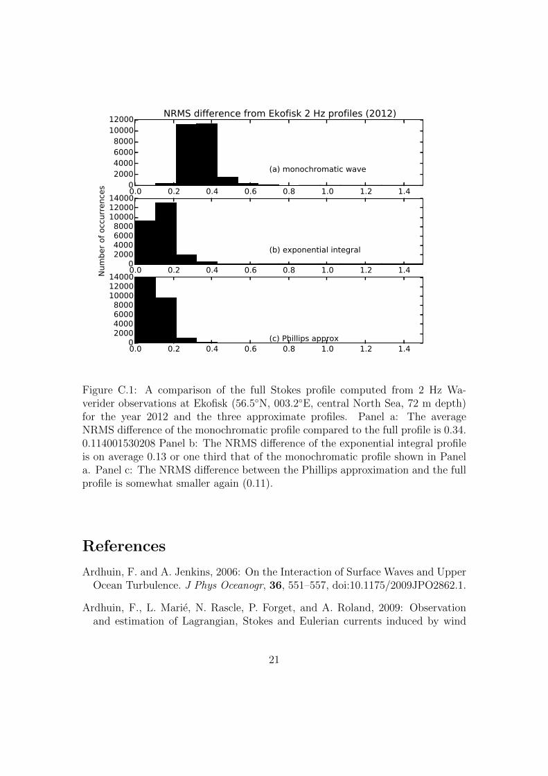
We have estimated the profile from the same observational spectra as was used byBJB from the Ekofisk location in the central North Sea for the period 2012 (morethan 24,000 spectra in total). The location is (56.5◦N, 003.2◦E). The samplingrate was 2 Hz and 20-minute spectra were computed as described by BJB. TheNRMS difference is shown in Fig C.1. As can be seen from Panel c, the new profilereduces the NRMS difference slightly compared with the exponential integral andquite dramatically compared with the monochromatic profile. It is worth notingthat no ω−5 tail has been fitted to the spectra, so the improvement is present evenwithout adding a high-frequency tail.

20

0.0 0.2 0.4 0.6 0.8 1.0 1.2 1.40

2000400060008000

1000012000

(a) monochromatic wave

NRMS difference from Ekofisk 2 Hz profiles (2012)

0.0 0.2 0.4 0.6 0.8 1.0 1.2 1.40

2000400060008000

100001200014000

Num

ber

of

occ

urr

ence

s

(b) exponential integral

0.0 0.2 0.4 0.6 0.8 1.0 1.2 1.40

2000400060008000

100001200014000

(c) Phillips approx

Figure C.1: A comparison of the full Stokes profile computed from 2 Hz Wa-verider observations at Ekofisk (56.5◦N, 003.2◦E, central North Sea, 72 m depth)for the year 2012 and the three approximate profiles. Panel a: The averageNRMS difference of the monochromatic profile compared to the full profile is 0.34.0.114001530208 Panel b: The NRMS difference of the exponential integral profileis on average 0.13 or one third that of the monochromatic profile shown in Panela. Panel c: The NRMS difference between the Phillips approximation and the fullprofile is somewhat smaller again (0.11).

References

Ardhuin, F. and A. Jenkins, 2006: On the Interaction of Surface Waves and UpperOcean Turbulence. J Phys Oceanogr, 36, 551–557, doi:10.1175/2009JPO2862.1.

Ardhuin, F., L. Marie, N. Rascle, P. Forget, and A. Roland, 2009: Observationand estimation of Lagrangian, Stokes and Eulerian currents induced by wind

21

and waves at the sea surface. J Phys Oceanogr, 39, 2820–2838, doi:10.1175/2009JPO4169.1.

Axell, L. B., 2002: Wind-driven internal waves and Langmuir circulations in anumerical ocean model of the southern Baltic Sea. J Geophys Res, 107 (C11),20, doi:10.1029/2001JC000922.

Babanin, A. V., 2006: On a wave-induced turbulence and a wave-mixed upperocean layer. Geophys Res Lett, 33 (20), 6, doi:10.1029/2006GL027308.

Babanin, A. V., A. Ganopolski, and W. R. Phillips, 2009: Wave-induced upper-ocean mixing in a climate model of intermediate complexity. Ocean Model,29 (3), 189–197, doi:10.1016/j.ocemod.2009.04.003.

Babanin, A. V. and B. K. Haus, 2009: On the existence of water turbulenceinduced by nonbreaking surface waves. J Phys Oceanogr, 39 (10), 2675–2679,doi:10.1175/2009JPO4202.1.

Belcher, S. E., et al., 2012: A global perspective on Langmuir turbulencein the ocean surface boundary layer. Geophys Res Lett, 39 (18), 9, doi:10.1029/2012GL052932.

Breivik, Ø., A. Allen, C. Maisondieu, and M. Olagnon, 2013: Advances in Searchand Rescue at Sea. Ocean Dyn, 63 (1), 83–88, arXiv:1211.0805, doi:10/jtx.

Breivik, Ø., A. Allen, C. Maisondieu, J.-C. Roth, and B. Forest, 2012: The Leewayof Shipping Containers at Different Immersion Levels. Ocean Dyn, 62 (5), 741–752, arXiv:1201.0603, doi:10.1007/s10236-012-0522-z, sAR special issue.

Breivik, Ø., P. Janssen, and J. Bidlot, 2014: Approximate Stokes Drift Profilesin Deep Water. J Phys Oceanogr, 44 (9), 2433–2445, arXiv:1406.5039, doi:10.1175/JPO-D-14-0020.1.

Breivik, Ø., K. Mogensen, J.-R. Bidlot, M. A. Balmaseda, and P. A. Janssen,2015: Surface Wave Effects in the NEMO Ocean Model: Forced and Cou-pled Experiments. J Geophys Res Oceans, 120, arXiv:1503.07 677, doi:10.1002/2014JC010565.

Carniel, S., M. Sclavo, L. H. Kantha, and C. A. Clayson, 2005: Langmuir cellsand mixing in the upper ocean. Il Nuovo Cimento C Geophysics Space PhysicsC, 28C, 33–54, doi:10.1393/ncc/i2005-10022-8.

22

Carrasco, A., A. Semedo, P. E. Isachsen, K. H. Christensen, and Ø. Saetra, 2014:Global surface wave drift climate from ERA-40: the contributions from wind-sea and swell. Ocean Dyn, 64 (12), 1815–1829, doi:10.1007/s10236-014-0783-9,13th wave special issue.

Craik, A., 1977: The generation of Langmuir circulations by an instability mech-anism. J Fluid Mech, 81, 209–223, doi:10.1017/S0022112077001980.

Craik, A. and S. Leibovich, 1976: A rational model for Langmuir circulations. JFluid Mech, 73 (03), 401–426, doi:10.1017/S0022112076001420.

Dee, D., et al., 2011: The ERA-Interim reanalysis: Configuration and performanceof the data assimilation system. Q J R Meteorol Soc, 137 (656), 553–597, doi:10.1002/qj.828.

Donelan, M. A., J. Hamilton, and W. H. Hui, 1985: Directional spectra of wind-generated waves. Phil Trans R Soc Lond A, 315, 509–562, doi:10.1098/rsta.1985.0054.

ECMWF, 2013: IFS Documentation CY40r1, Part VII: ECMWF Wave Model.ECMWF Model Documentation, European Centre for Medium-Range WeatherForecasts, 79 pp, available at http://old.ecmwf.int/research/ifsdocs/CY40r1/pp.

Faller, A. J. and E. A. Caponi, 1978: Laboratory studies of wind-drivenLangmuir circulations. J Geophys Res, 83 (C7), 3617–3633, doi:10.1029/JC083iC07p03617.

Fan, Y. and S. M. Griffies, 2014: Impacts of parameterized Langmuir turbulenceand non-breaking wave mixing in global climate simulations. J Climate, doi:10.1175/JCLI-D-13-00583.1.

Flor, J. B., E. J. Hopfinger, and E. Guyez, 2010: Contribution of coherent vor-tices such as Langmuir cells to wind-driven surface layer mixing. J Geophys ResOceans, 115 (C10), doi:10.1029/2009JC005900, c10031.

Gradshteyn, I. and I. Ryzhik, 2007: Table of Integrals, Series, and Products, 7thedition. Edited by A. Jeffrey and D. Zwillinger, Academic Press, London, 1221pp.

Grant, A. L. and S. E. Belcher, 2009: Characteristics of Langmuir turbulencein the ocean mixed layer. J Phys Oceanogr, 39 (8), 1871–1887, doi:10.1175/2009JPO4119.1.

23

Hasselmann, K., 1970: Wave-driven inertial oscillations. Geophys Astrophys FluidDyn, 1 (3-4), 463–502, doi:10.1080/03091927009365783.

Hasselmann, K., et al., 1973: Measurements of wind-wave growth and swell de-cay during the Joint North Sea Wave Project (jonswap). Deutsch Hydrogr Z,A8 (12), 1–95.

Huang, C. J., F. Qiao, Z. Song, and T. Ezer, 2011: Improving simulations ofthe upper ocean by inclusion of surface waves in the Mellor-Yamada turbulencescheme. J Geophys Res, 116 (C1), doi:10.1029/2010JC006320.

Janssen, P., 2012: Ocean Wave Effects on the Daily Cycle in SST. J Geophys ResOceans, 117, 24, doi:10/mth.

Janssen, P., O. Saetra, C. Wettre, H. Hersbach, and J. Bidlot, 2004: Impact ofthe sea state on the atmosphere and ocean. Annales hydrographiques, Servicehydrographique et oceanographique de la marine, Vol. 3-772, 3.1–3.23.

Janssen, P., et al., 2013: Air-Sea Interaction and Surface Waves. ECMWF Techni-cal Memorandum 712, European Centre for Medium-Range Weather Forecasts,36 pp.

Jenkins, A. D., 1987: Wind and wave induced currents in a rotating sea withdepth-varying eddy viscosity. J Phys Oceanogr, 17, 938–951, doi:10/fdwvq2.

Kantha, L. H. and C. A. Clayson, 2000: Small scale processes in geophysical fluidflows, Vol. 67. Academic Press.

Kantha, L. H. and C. A. Clayson, 2004: On the effect of surface gravity waves onmixing in the oceanic mixed layer. Ocean Model, 6 (2), 101–124, doi:10.1016/S1463-5003(02)00062-8.

Kenyon, K. E., 1969: Stokes Drift for Random Gravity Waves. J Geophys Res,74 (28), 6991–6994, doi:10.1029/JC074i028p06991.

Langmuir, I., 1938: Surface motion of water induced by wind. Science, 87 (2250),119–123, doi:10.1126/science.87.2250.119.

Large, W. G., J. C. McWilliams, and S. C. Doney, 1994: Oceanic vertical mixing:A review and a model with a nonlocal boundary layer parameterization. RevGeophys, 32 (4), 363–403, doi:10.1029/94RG01872.

Leibovich, S., 1977: Convective instability of stably stratified water in the ocean.J Fluid Mech, 82, 561–581, doi:10.1017/S0022112077000846.

24

Leibovich, S., 1980: On wave-current interaction theories of Langmuir circulations.J Fluid Mech, 99, 715–724, doi:10.1017/S0022112080000857.

Leibovich, S., 1983: The form and dynamics of Langmuir circulations. Annu RevFluid Mech, 15 (1), 391–427, doi:10.1146/annurev.fl.15.010183.002135.

Li, M. and C. Garrett, 1997: Mixed layer deepening due to Langmuir circulation.J Phys Oceanogr, 27 (1), 121–132, doi:10/cmhvrr.

Li, Q., A. Webb, B. Fox-Kemper, A. Craig, G. Danabasoglu, W. G. Large, andM. Vertenstein, 2015: Langmuir mixing effects on global climate: WAVE-WATCH III in CESM. Ocean Model, doi:10.1016/j.ocemod.2015.07.020.

McWilliams, J., P. Sullivan, and C.-H. Moeng, 1997: Langmuir turbulence in theocean. J Fluid Mech, 334 (1), 1–30, doi:10.1017/S0022112096004375.

McWilliams, J. C., E. Huckle, J. Liang, and P. Sullivan, 2014: Langmuir turbulencein swell. J Phys Oceanogr, 44, 870–890, doi:10.1175/JPO-D-13-0122.1.

McWilliams, J. C. and J. M. Restrepo, 1999: The Wave-driven Ocean Circulation.J Phys Oceanogr, 29 (10), 2523–2540, doi:10/dwj9tj.

McWilliams, J. C. and P. P. Sullivan, 2000: Vertical mixing by Langmuir cir-culations. Spill Science and Technology Bulletin, 6 (3), 225–237, doi:10.1016/S1353-2561(01)00041-X.

Phillips, O. M., 1958: The equilibrium range in the spectrum of wind-generatedwaves. J Fluid Mech, 4, 426–434, doi:10.1017/S0022112058000550.

Pierson, W. J., Jr and L. Moskowitz, 1964: A proposed spectral form for fullydeveloped wind seas based on the similarity theory of S A Kitaigorodskii. JGeophys Res, 69, 5181–5190.

Polton, J. A., D. M. Lewis, and S. E. Belcher, 2005: The role of wave-inducedCoriolis-Stokes forcing on the wind-driven mixed layer. J Phys Oceanogr, 35 (4),444–457, doi:10.1175/JPO2701.1.

Qiao, F., Y. Yuan, T. Ezer, C. Xia, Y. Yang, X. Lu, and Z. Song, 2010: A three-dimensional surface wave–ocean circulation coupled model and its initial testing.Ocean Dyn, 60 (5), 1339–1355, doi:10.1007/s10236-010-0326-y.

Qiao, F., Y. Yuan, Y. Yang, Q. Zheng, C. Xia, and J. Ma, 2004: Wave-inducedmixing in the upper ocean: Distribution and application to a global ocean cir-culation model. Geophys Res Lett, 31 (11), 4, doi:10.1029/2004GL019824.

25

Rascle, N. and F. Ardhuin, 2013: A global wave parameter database for geophysicalapplications. Part 2: Model validation with improved source term parameteri-zation. Ocean Model, 70, 174–188, doi:10.1016/j.ocemod.2012.12.001.

Rascle, N., F. Ardhuin, P. Queffeulou, and D. Croize-Fillon, 2008: A globalwave parameter database for geophysical applications. Part 1: Wave-current-turbulence interaction parameters for the open ocean based on traditional pa-rameterizations. Ocean Model, 25 (3–4), 154–171, doi:10.1016/j.ocemod.2008.07.006.

Rascle, N., F. Ardhuin, and E. Terray, 2006: Drift and mixing under the oceansurface: A coherent one-dimensional description with application to unstratifiedconditions. J Geophys Res, 111 (C3), 16, doi:10.1029/2005JC003004.

Reistad, M., Ø. Breivik, H. Haakenstad, O. J. Aarnes, B. R. Furevik, and J.-R.Bidlot, 2011: A high-resolution hindcast of wind and waves for the North Sea,the Norwegian Sea, and the Barents Sea. J Geophys Res Oceans, 116, 18 pp,C05 019, arXiv:1111.0770, doi:10/fmnr2m.

Rohrs, J., K. Christensen, L. Hole, G. Brostrom, M. Drivdal, and S. Sundby, 2012:Observation-based evaluation of surface wave effects on currents and trajectoryforecasts. Ocean Dyn, 62 (10–12), 1519–1533, doi:10.1007/s10236-012-0576-y,sAR special issue.

Rohrs, J., A. Sperrevik, K. Christensen, Ø. Breivik, and G. Brostrom, 2015: Com-parison of HF radar measurements with Eulerian and Lagrangian surface cur-rents. Ocean Dyn, 1–12, doi:10.1007/s10236-015-0828-8.

Saetra, Ø., J. Albretsen, and P. Janssen, 2007: Sea-State-Dependent MomentumFluxes for Ocean Modeling. J Phys Oceanogr, 37 (11), 2714–2725, doi:10.1175/2007JPO3582.1.

Semedo, A., R. Vettor, Ø. Breivik, A. Sterl, M. Reistad, C. G. Soares, and D. C. A.Lima, 2015: The Wind Sea and Swell Waves Climate in the Nordic Seas. OceanDyn, 65 (2), 223–240, doi:10.1007/s10236-014-0788-4, 13th wave special issue.

Sheldon, L. and A. Czaja, 2014: Seasonal and interannual variability of an indexof deep atmospheric convection over western boundary currents. Q J R MeteorolSoc, 140 (678), 22–30, doi:10.1002/qj.2103.

Skyllingstad, E. D. and D. W. Denbo, 1995: An ocean large-eddy simulation ofLangmuir circulations and convection in the surface mixed layer. J Geophys Res,100 (C5), 8501–8522, doi:10.1029/94JC03202.

26

Stokes, G. G., 1847: On the theory of oscillatory waves. Trans Cambridge PhilosSoc, 8, 441–455.

Stull, R. B., 1988: An introduction to boundary layer meteorology. Kluwer, NewYork, 666 pp.

Tamura, H., Y. Miyazawa, and L.-Y. Oey, 2012: The Stokes drift and waveinduced-mass flux in the North Pacific. J Geophys Res, 117 (C8), 14, doi:10.1029/2012JC008113.

Thorpe, S., 2004: Langmuir Circulation. Annu Rev Fluid Mech, 36, 55–79, doi:10.1146/annurev.fluid.36.052203.071431.

Webb, A. and B. Fox-Kemper, 2011: Wave spectral moments and Stokes driftestimation. Ocean Model, 40, 273–288, doi:10.1016/j.ocemod.2011.08.007.

Webb, A. and B. Fox-Kemper, 2015: Impacts of wave spreading and multidirec-tional waves on estimating Stokes drift. Ocean Model, 16, doi:10.1016/j.ocemod.2014.12.007.

Weber, J. E., 1983: Steady Wind- and Wave-Induced Currents in the Open Ocean.J Phys Oceanogr, 13, 524–530, doi:10/djz6md.

27