PANM 14

Pavel Burda; Jaroslav Novotný; Jakub Šístek; Alexandr DamašekFinite element modelling of some incompressible fluid flow problems

In: Jan Chleboun and Petr Přikryl and Karel Segeth and Tomáš Vejchodský (eds.): Programs and Algorithms ofNumerical Mathematics, Proceedings of Seminar. Dolní Maxov, June 1-6, 2008. Institute of Mathematics AS CR,Prague, 2008. pp. 37–52.

Persistent URL: http://dml.cz/dmlcz/702854

Terms of use:© Institute of Mathematics AS CR, 2008

Institute of Mathematics of the Czech Academy of Sciences provides access to digitized documents strictly forpersonal use. Each copy of any part of this document must contain these Terms of use.

This document has been digitized, optimized for electronic delivery and stamped withdigital signature within the project DML-CZ: The Czech Digital Mathematics Libraryhttp://dml.cz

FINITE ELEMENT MODELLING OF SOME INCOMPRESSIBLEFLUID FLOW PROBLEMS∗

Pavel Burda, Jaroslav Novotny, Jakub Sıstek, Alexandr Damasek

Abstract

We deal with modelling of flows in channels or tubes with abrupt changes of thediameter. The goal of this work is to construct the FEM solution in the vicinity ofthese corners as precise as desired. We present two ways. The first approach makesuse of a posteriori error estimates and the adaptive strategy. The second approach isbased on the asymptotic behaviour of the exact solution in the vicinity of the cornerand on the a priori error estimate of the FEM solution. Then we obtain the solutionwith desired precision also in the vicinity of the corner, though there is a singularity.Numerical results are demonstrated on a 2D example.

1. Introduction

One of the challenging problems in fluid dynamics is reliable modelling of flowsin channels or tubes with abrupt changes of the diameter, which appear often inengineering practice.

We present two ways for getting desired precision of the FEM solution in thevicinity of corners. Both make use of qualitative properties of the mathematicalmodel of flow that is on the Navier-Stokes equations (NSE) for incompressible fluids.

The first approach makes use of a posteriori error estimates of the FEM solutionwhich is carefully derived to trace the quality of the solution. Especially the constantin the a posteriori error estimate is investigated with care. Then we use the adaptivestrategy to improve the mesh and thus to improve the FEM solution.

The second approach stands on two legs. One is the asymptotic behaviour of theexact solution of the NSE in the vicinity of the corner. This is obtained using somesymmetry of the principal part of the Stokes equation and application of the Fouriertransform. Second leg is the a priori error estimate of the FEM solution, wherewe estimate the seminorm of the exact solution by means of the above obtainedasymptotics. On the mesh we then obtain the solution with desired precision also inthe vicinity of the corner, though there is a singularity.

2. Navier-Stokes equations for incompressible viscous fluids

Let Ω be an open bounded domain in R2 filled with a fluid and let Γ be itsLipschitz continuous boundary. The generic point of R2 is denoted by x = (x1, x2)

T

considered in meters and t denotes time variable considered in seconds.

∗This work was supported by grant No. 106/08/0403 of the Czech Science Foundation and bythe State Research Project No. MSM 684 0770010.

37

2.1. Unsteady two-dimensional flow

We deal with isothermal flow of Newtonian viscous fluids with constant density.Such flow is modelled by the Navier-Stokes system (nonconservative form):

ρ

(∂u

∂t+ (u · ∇)u

)− µ∆u +∇pr = ρ f in Ω× [0, T ], (1)

∇ · u = 0 in Ω× [0, T ], (2)

where

• u = (u1, u2)T denotes the vector of flow velocity [m/s], it is a function of

x and t,

• pr denotes the pressure [Pa], which is a function of x and t,

• ρ denotes the density of the fluid [kg/m3],

• µ denotes the dynamic viscosity of the fluid [Pa·s], supposed to be constant,

• f = f(x, t) is the density of volume forces per mass unit [N/m3].

Dividing both sides of the momentum equation (1) by ρ and leaving the continuityequation (2) unchanged we obtain

∂u

∂t+ (u · ∇)u− ν∆u +∇p = f in Ω× [0, T ], (3)

∇ · u = 0 in Ω× [0, T ], (4)

where

• p = pr/ρ denotes the pressure divided by the density [Pa· m3 /kg],

• ν = µ/ρ denotes the kinematic viscosity of the fluid [m2/s].

The system is supplied with the initial condition

u = u0 in Ω, t = 0, (5)

where ∇ · u0 = 0 and with the boundary conditions

u = g on Γg × [0, T ], (6)

−ν(∇u)n + pn = 0 on Γh × [0, T ], (7)

where

• Γg and Γh are two subsets of Γ satisfying Γ = Γg ∪ Γh, µR1(Γg ∩ Γh) = 0,

• n denotes the unit outer normal vector to the boundary Γ.

Introduced g is a given function of x and t satisfying in the case of Γ = Γg for allt ∈ [0, T ]

∫

Γ

g · n dΓ = 0.

38

2.2. Steady 2D Navier-Stokes problem

In the case of steady two-dimensional flow, the Navier-Stokes equations are re-duced to

(u · ∇)u− ν∆u +∇p = f in Ω, (8)

∇ · u = 0 in Ω (9)

and boundary conditions to

u = g on Γg, (10)

−ν(∇u)n + pn = 0 on Γh. (11)

2.3. Steady 2D Stokes problem

In the case of the Stokes flow the first (nonlinear) term in (8) is omitted:

−ν∆u +∇p = f in Ω , (12)

∇ · u = 0 in Ω (13)

and boundary conditions are the same as in (10), (11).

2.4. Variational formulation of Navier-Stokes equations

Let L2(Ω) be the space of square integrable functions on Ω and let L2(Ω)/R bethe space of functions in L2(Ω) ignoring an additive constant. Let H1(Ω) and H1

0 (Ω)be the Sobolev spaces defined as

H1(Ω) ≡

v | v ∈ L2(Ω),∂v

∂xi

∈ L2(Ω), i = 1, 2

,

H10 (Ω) ≡

v | v ∈ H1(Ω),Tr v = 0

,

where Tr is the trace operator Tr : H1(Ω) −→ L2(Γ) and derivatives are consideredin the weak sense.

The inner product and norm in the space L2(Ω) are defined as

(u, v)L2(Ω) ≡∫

Ω

uv dΩ , ‖v‖2L2(Ω) ≡

∫

Ω

v2dΩ

and the norm of function v in the Sobolev space H1(Ω) is considered as

‖v‖2H1(Ω) ≡

∫

Ω

(v2 +

2∑

k=1

(∂v

∂xk

)2)

dΩ .

Sometimes, the notation ‖·‖L2(Ω) is shortened to ‖·‖0 and ‖·‖H1(Ω) to ‖·‖1. Similarly,the notation (u, v)L2(Ω) is shortened to (u, v)0.

39

Let us define vector function spaces Vg and V by

Vg ≡v = (v1, v2)

T | v ∈ [H1(Ω)]2;Tr vi = gi, i = 1, 2

,

V ≡v = (v1, v2)

T | v ∈ [H10 (Ω)]2

.

Let us note, that the norm of vector function v in the spaces Vg and V is then

‖v‖2[H1(Ω)]2 ≡

2∑i=1

∫

Ω

(v2

i +2∑

k=1

(∂vi

∂xk

)2)

dΩ

and the norm of vector function v in the space [L2(Ω)]2 is

‖v‖2[L2(Ω)]2 ≡

2∑i=1

∫

Ω

v2i dΩ .

The weak unsteady Navier-Stokes problem means seeking of u(t) ∈ Vg, u(t) =(u1(t), u2(t))

T , and p(t) ∈ L2(Ω)/R satisfying for any t ∈ [0, T ] and ∀ v ∈ V and∀ ψ ∈ L2(Ω):

∫

Ω

∂u

∂t· vdΩ +

∫

Ω

(u · ∇)u · vdΩ +ν

∫

Ω

∇u : ∇vdΩ−∫

Ω

p∇ · vdΩ =

∫

Ω

f · vdΩ ,

(14)∫

Ω

ψ∇ · udΩ = 0 , (15)

u− ug ∈ V. (16)

The operation ∇u : ∇v is defined as

∇u : ∇v ≡ ∂ux

∂x

∂vx

∂x+

∂ux

∂y

∂vx

∂y+

∂uy

∂x

∂vy

∂x+

∂uy

∂y

∂vy

∂y.

Similarly, the weak steady Navier-Stokes problem reads:Seek u = (u1, u2)

T ∈ Vg and p ∈ L2(Ω)/R satisfying ∀ v ∈ V and ∀ ψ ∈ L2(Ω):∫

Ω

(u · ∇)u · vdΩ + ν

∫

Ω

∇u : ∇vdΩ−∫

Ω

p∇ · vdΩ =

∫

Ω

f · vdΩ , (17)∫

Ω

ψ∇ · udΩ = 0 , (18)

u− ug ∈ V. (19)

In case of the weak steady Stokes problem instead of (17) we require

ν

∫

Ω

∇u : ∇vdΩ−∫

Ω

p∇ · vdΩ =

∫

Ω

f · vdΩ . (20)

40

3. Finite element method for Navier-Stokes equations

Let us divide the domain Ω (supposed to be polygonal from now) into N elementsTK , K = 1, 2, . . . , N , of a triangulation T such that

N⋃K=1

TK = Ω ,

µR2 (TK ∩ TL) = 0, K 6= L .

Let hK mean the diameter of the element TK .

3.1. Function spaces for velocity and pressure approximation

To solve the Navier-Stokes equations, different polynomial approximation for ve-locities and for pressure are usually chosen. Equal order approximation is easy toimplement, but pressure exhibits instability. Approximation with different order ismore suitable for practical computing, cf. [3]. I. Babuska and F. Brezzi introduceda condition (also called inf -sup condition) limitting the choice of combinations ofapproximation

∃CB > 0, const. ∀qh ∈ Qh ∃vh ∈ Vgh (qh,∇ · vh)0 ≥ CB‖qh‖0‖vh‖1 , (21)

where Qh and Vgh are the function spaces for approximation of pressure and velocity.Condition (21) is important for stability. It is satisfied, e.g., for Taylor-Hood elementswe use.

3.2. Taylor-Hood finite elements

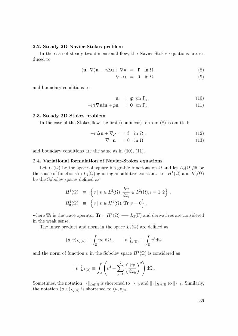
In this paper we apply Taylor-Hood finite elements on triangles and quadrilater-als. Values of velocity are approximated at corner nodes and midsides and values ofpressure at corner nodes (Figure 1). It corresponds to the following function spaceson element TK :

• trianglevi ∈ P2(TK), i = 1, 2, i.e. polynomials of the second order,p ∈ P1(TK), i.e. linear polynomials

• quadrilateralvi ∈ Q2(TK), i = 1, 2, i.e. polynomials of the second order for each coordinate,p ∈ Q1(TK), i.e. bilinear polynomials.

Let us employ the notation

Rm(TK) =

Pm(TK), if TK is a triangleQm(TK), if TK is a quadrilateral

(22)

and let C(Ω) denote the space of continuous functions on Ω.

41

-6

-

6

Æ u Æ uÆ uÆ u

vx; vy; p vx; vy; pvx; vy; pvx; vy; p

vx; vy vx; vyvx; vyvx; vy

1 234

8 657

Æ Æ Æ Æ

-6-6

-6-6

-6 -6-6

-6 Æ u Æ uÆ u@@@@@@ @@@@@@Æ

Æ Æ vx; vy; p vx; vy; p

vx; vy; pvx; vy vx; vy

vx; vy1 23

6 54-6

-6

-6-6 -6-6

Fig. 1: Taylor-Hood reference elements.

Application of Taylor-Hood finite elements leads to the final approximation onthe domain Ω satisfying uh ∈ Vgh and ph ∈ Qh where

Vgh =vh = (vh1 , vh2)

T ∈ [C(Ω)]2; vhi|TK∈ R2(TK), K = 1, . . . , N, i = 1, 2, (23)

vh = g at nodes on Γ

,

Qh =

ψh ∈ C(Ω); ψh |TK∈ R1(TK), K = 1, . . . , N

. (24)

We also need the space

Vh =vh = (vh1 , vh2)

T ∈ [C(Ω)]2; vhi|TK∈ R2(TK), K = 1, . . . , N, i = 1, 2, (25)

vh = 0 at nodes on Γ

.

Since these spaces satisfy Vgh ⊂ Vg, Vh ⊂ V , and Qh ⊂ L2(Ω)/R for prescribedarbitrary value of pressure (e.g. ph = 0) in one node, we can introduce approximatesteady Navier-Stokes problem:Seek uh ∈ Vgh and ph ∈ Qh satisfying∫

Ω

(uh · ∇)uh · vhdΩ + ν

∫

Ω

∇uh : ∇vhdΩ−∫

Ω

ph∇ · vhdΩ =

∫

Ω

f · vhdΩ, ∀vh ∈ Vh,

(26)∫

Ω

ψh∇ · uhdΩ = 0, ∀ψh ∈ Qh , (27)

uh − ugh ∈ Vh , (28)

where ugh ∈ Vgh is the projection of ug onto the space Vgh.

42

Similarly we define approximate steady Stokes problem, just omitting the firstterm in (26).

Using the shape-regular triangulation and refining the mesh such that hmax → 0,where

hmax = maxK

hK ,

the solution of the approximated problem converges to the solution of the continuousproblem (for more detail see e.g. [3]).

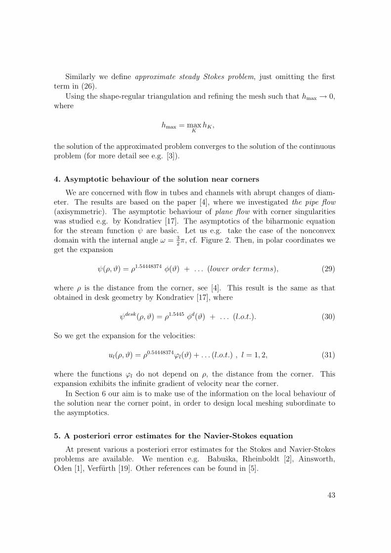
4. Asymptotic behaviour of the solution near corners

We are concerned with flow in tubes and channels with abrupt changes of diam-eter. The results are based on the paper [4], where we investigated the pipe flow(axisymmetric). The asymptotic behaviour of plane flow with corner singularitieswas studied e.g. by Kondratiev [17]. The asymptotics of the biharmonic equationfor the stream function ψ are basic. Let us e.g. take the case of the nonconvexdomain with the internal angle ω = 3

2π, cf. Figure 2. Then, in polar coordinates we

get the expansion

ψ(ρ, ϑ) = ρ1.54448374 φ(ϑ) + . . . (lower order terms), (29)

where ρ is the distance from the corner, see [4]. This result is the same as thatobtained in desk geometry by Kondratiev [17], where

ψdesk(ρ, ϑ) = ρ1.5445 φd(ϑ) + . . . (l.o.t.). (30)

So we get the expansion for the velocities:

ul(ρ, ϑ) = ρ0.54448374ϕl(ϑ) + . . . (l.o.t.) , l = 1, 2, (31)

where the functions ϕl do not depend on ρ, the distance from the corner. Thisexpansion exhibits the infinite gradient of velocity near the corner.

In Section 6 our aim is to make use of the information on the local behaviour ofthe solution near the corner point, in order to design local meshing subordinate tothe asymptotics.

5. A posteriori error estimates for the Navier-Stokes equation

At present various a posteriori error estimates for the Stokes and Navier-Stokesproblems are available. We mention e.g. Babuska, Rheinboldt [2], Ainsworth,Oden [1], Verfurth [19]. Other references can be found in [5].

43

5.1. A posteriori estimates for 2D steady Navier-Stokes equations

Let us consider the steady Navier-Stokes problem (8), (9), with boundary condi-tions (10), (11).

For the discretization by finite elements we use again Taylor-Hood elementsP2/P1.

Suppose that exact solution of the problem is denoted by (u1, u2, p) and theapproximate finite element solution by (uh

1 , uh2 , ph). The exact solution differs from

the approximate solution in the error

(eu1 , eu2 , ep) ≡ (u1 − uh1 , u2 − uh

2 , p− ph). (32)

For the solution (u1, u2, p) we denote

U2(u1, u2, p, Ω) ≡ ‖(u1, u2, p)‖2V ≡ ‖(u1, u2)‖2

1,Ω + ‖p‖20,Ω (33)

≡∫

Ω

(u2

1 + u22 +

(∂u1

∂x

)2

+

(∂u1

∂y

)2

+

(∂u2

∂x

)2

+

(∂u2

∂y

)2)

dΩ +

∫

Ω

p2dΩ.

The estimate proved in [5], [6], [7] for the Stokes problem can be generalized to theNavier-Stokes equations:

‖(eu1 , eu2)‖21,Ω + ‖ep‖2

0,Ω ≤ E2(uh1 , u

h2 , p

h), (34)

where (cf. [19])

E2(uh1 , u

h2 , p

h, Ω) ≡ C

[ ∑

K∈T h

h2K

∫

TK

(r21 + r2

2

)+

∑

K∈T h

∫

TK

r23dΩ

], (35)

where hK denotes the diameter of the element TK and ri, i = 1, 2, 3, are the residuals

r1 = fx −(

uh1

∂uh1

∂x+ u2

∂uh1

∂y

)+ ν

(∂2uh

1

∂x2+

∂2uh1

∂y2

)− ∂ph

∂x, (36)

r2 = fy −(

uh1

∂uh2

∂x+ uh

2

∂uh2

∂y

)+ ν

(∂2uh

2

∂x2+

∂2uh2

∂y2

)− ∂ph

∂y, (37)

r3 =∂uh

1

∂x+

∂uh2

∂y. (38)

Let us note that due to our practical experience we use only the element residuals.Denote also

E2(uh1 , u

h2 , p

h, TK) ≡ C

[h2

K

∫

TK

(r21 + r2

2

)+

∫

TK

r23dΩ

]. (39)

It is important, that C does not depend on the mesh size and so can be determinedexperimentally for general situation.

44

By computing of the estimates (11) we obtain absolute numbers, that will dependon given quantities in different problems. We are mainly interested in the errorrelated to the computed solution, i.e. relative error. This is given by the ratio ofthe absolute norm of the solution error related to the unit area of the element TK ,

1|TK | E2(uh

1 , uh2 , p

h, TK), and the solution norm on the whole domain Ω, related to unit

area 1|Ω| ‖(uh

1 , uh2 , p

h)‖2V,Ω, i.e.

R2(uh1 , u

h2 , p

h, TK) =|Ω| E2(uh

1 , uh2 , p

h, TK)

|TK | ‖(uh1 , u

h2 , p

h)‖2V,Ω

. (40)

5.2. Determination of the constant C

In papers [7], [8] we investigated the problem of the constant C in the a posterioriestimates. Comparing analytical and finite element solution of some model problemswe found the appropriate value of the constant. For details we refer to [7] and [8].

5.3. Numerical results and application of estimates to the construction ofadaptive meshes

Consider two-dimensional flow of viscous, incompressible fluid described byNavier-Stokes equations in domain with corner singularity, cf. Figure 2.

Fig. 2: Geometry of the channel.

Due to the symmetry, we solve the problem only on half of the channel, cf. Fig-ure 3. On the inflow we consider parabolic velocity profile, on the outflow ‘do nothing’boundary condition. On the upper wall no-slip condition and on the lower wall con-dition of symmetry (i.e. only y-component of velocity equals zero). We consider thefollowing parameters: ν = 0.0001 m2/s, uin = 1 m/s. The initial mesh is in Figure 3.

Fig. 3: Initial finite element mesh.

Elements, where the relative error by (40) exceeds 3%, are refined and newsolution together with new error estimates is computed. The third refinement isseen in Figure 4.

The relative errors in the vicinity of the left corner are shown in Figure 5.

45

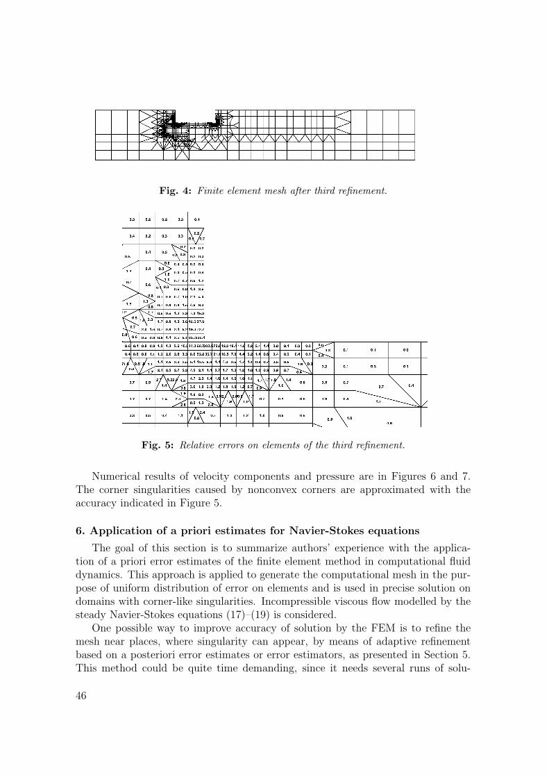
Fig. 4: Finite element mesh after third refinement.

Fig. 5: Relative errors on elements of the third refinement.

Numerical results of velocity components and pressure are in Figures 6 and 7.The corner singularities caused by nonconvex corners are approximated with theaccuracy indicated in Figure 5.

6. Application of a priori estimates for Navier-Stokes equations

The goal of this section is to summarize authors’ experience with the applica-tion of a priori error estimates of the finite element method in computational fluiddynamics. This approach is applied to generate the computational mesh in the pur-pose of uniform distribution of error on elements and is used in precise solution ondomains with corner-like singularities. Incompressible viscous flow modelled by thesteady Navier-Stokes equations (17)–(19) is considered.

One possible way to improve accuracy of solution by the FEM is to refine themesh near places, where singularity can appear, by means of adaptive refinementbased on a posteriori error estimates or error estimators, as presented in Section 5.This method could be quite time demanding, since it needs several runs of solu-

46

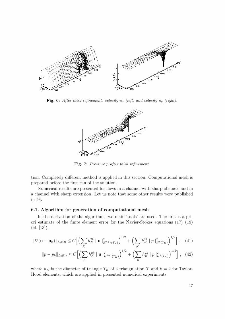
Fig. 6: After third refinement: velocity ux (left) and velocity uy (right).

Fig. 7: Pressure p after third refinement.

tion. Completely different method is applied in this section. Computational mesh isprepared before the first run of the solution.

Numerical results are presented for flows in a channel with sharp obstacle and ina channel with sharp extension. Let us note that some other results were publishedin [9].

6.1. Algorithm for generation of computational mesh

In the derivation of the algorithm, two main ‘tools’ are used. The first is a pri-ori estimate of the finite element error for the Navier-Stokes equations (17)–(19)(cf. [13]),

‖∇(u− uh)‖L2(Ω) ≤ C[(∑

K

h2kK | u |2

Hk+1(TK)

)1/2

+(∑

K

h2kK | p |2Hk(TK)

)1/2], (41)

‖p− ph‖L2(Ω) ≤ C[(∑

K

h2kK | u |2

Hk+1(TK)

)1/2

+(∑

K

h2kK | p |2Hk(TK)

)1/2], (42)

where hK is the diameter of triangle TK of a triangulation T and k = 2 for Taylor-Hood elements, which are applied in presented numerical experiments.

47

The second tool is the asymptotic behaviour of the solution near the singularity.In Section 4.2 (see also [4]), it was proved for the Stokes flow in axisymmetric tubes,that for internal angle α = 3

2π, the leading term of expansion of the solution for each

velocity component is

ui(ρ, ϑ) = ρ0.5445ϕi(ϑ) + . . . (l.o.t.), i = 1, 2 , (43)

where ρ is the distance from the corner, ϑ is the angle and ϕi is a smooth function.The same expansion is known to apply to the plane flow (cf. [16]) and similar resultswere also proved for the Navier-Stokes equations. Differentiating by ρ, we observe∂ui(ρ,ϑ)

∂ρ→ ∞ for ρ → 0.

Taking into account the expansion (43), we can estimate

| u |2Hk+1(TK)≈ C

rK∫

rK−hK

ρ2(γ−k−1) ρ dρ = C[−r

2(γ−k)K + (rK − hK)2(γ−k)

], (44)

where rK is the distance of element TK from the corner, cf. Figure 8.Putting estimate (44) into the a priori error estimate (41) or (42), we derive that

we should guarantee

h2kK

[−r

2(γ−k)K + (rK − hK)2(γ−k)

]≈ h2k

ref , (45)

in order to get the error estimate of order O(hkref ) uniformly distributed on elements.

From this expression, we compute element diameters using the Newton method inaccordance to chosen href . Similar idea was presented by C. Johnson for an ellipticproblem in [15].

6.2. Geometry and design of the mesh

The algorithm was applied to the channel with sudden intake of diameter (seeFigure 2). Due to symmetry, again the problem was solved only on the upper halfof the channel.

The diameters of elements were computed for values href = 0.1732 mm, k = 2,γ = 0.5444837. We started in the distance r1 = 0.25 mm from the corner. Thiscorresponds to cca 3% of relative error on elements. Fourteen diameters of elementswere obtained. The detail of the mesh refinement is in Figure 8. More in [8].

The refined detail is connected to the rest of the coarse mesh. In Figure 9 finalmesh after the refinement is shown.

6.3. Measuring of error

To review the efficiency of the algorithm, we use a posteriori error estimates asderived in Chapter 5, to evaluate the obtained error on elements. Suppose that theexact solution of the problem is denoted as (u1, u2, p) and the approximate solution

48

Fig. 8: Description of element variables (left), details of refined mesh (right).

0 0.05 0.1 0.150

0.02

Fig. 9: Final computational mesh for the channel.

obtained by the FEM as (uh1 , u

h2 , p

h). The exact solution differs from the approximatesolution in the error (eu1 , eu2 , ep) = (u1 − uh

1 , u2 − uh2 , p− ph).

In adaptive mesh refinement in Sections 5.3–5.5 we used the error estimator (40).In this chapter, for the similarity with a priori error estimate, we use the modifiedabsolute error defined as

A2m(u1h, u2h, ph, TK , Ω, n) =

|Ω|E2(u1h, u2h, ph, TK)

|TK | U2(u1h, u2h, ph, Ω), (46)

where |TK | is the mean area of elements obtained as |TK | = |Ω|n

, where n de-notes the number of all elements in the domain and the symbols E2(u1h, u2h, ph, TK),U2(u1h, u2h, ph, Ω) are defined in (33), (39).

6.4. Numerical results

Channel with sudden intake of diameter (results for Re = 1000)

In Figures 10-11, plots of entities that characterize the flow in the channel arepresented. In Figure 10, there are streamlines and a plot of the velocity componentux. Plots of velocity component uy and pressure are in Figure 11. Note, that the fluidflows from the right to the left on plots of ux, uy, and p for better view. Let us notethat the relative error on the elements never exceeded 3%. So the corner singularitiescaused by nonconvex corners are approximated here with very high accuracy.

7. Conclusion

Presented work is mainly focused on flow problems with singularities caused bycorners in the solution domain and on the construction of the FEM solution in thevicinity of these corners as precisely as desired.

49

Fig. 10: Detail of streamlines (left) and velocity component ux (right).

Fig. 11: Velocity component uy (left) and pressure (right).

We presented two ways for getting desired precision of the FEM solution in thevicinity of corners. Both make use of qualitative properties of the mathematicalmodel of flow. As a mathematical model we accept the Navier-Stokes equations(NSE) for incompressible fluids.

The first approach described in Section 5 makes use of a posteriori error estimatesof the FEM solution which is carefully derived to trace the quality of the solution.Especially the constant in the a posteriori estimate is investigated with care. Thenwe use the adaptive strategy to improve the mesh and thus to improve the FEMsolution. Numerical results demonstrate the robustness of this approach.

The second approach stands on two columns. In Section 4 we gave the asymptoticbehaviour of the exact solution of the NSE in the vicinity of the corner. This isobtained using some symmetry of the principal part of the Stokes equation, thenapplying the Fourier transform and investigating the resolvent of the correspondingoperator. Second column is the a priori error estimate of the FEM solution, wherewe estimate the seminorm of the exact solution by means of the above obtainedasymptotics. In Section 6, according to these ideas, we derive an algorithm fordesigning the FEM mesh in advance (a priori). On the mesh we then obtain the

50

solution with desired precision, namely in the vicinity of the corner, though there isa singularity.

The applications in Section 6 confirm the achievement of the goal – to obtainsolution tinged with errors on elements satisfactorily small and uniformly distributed.Using this approach, we can save a lot of computational time using mesh ‘prepared’for expected solution.

Recently we dealt also with the stabilized version of FEM to enable the calculationof flows with higher Reynolds numbers [10], [11]. We also combined stabilizationwith presented achievements on a posteriori error estimates. Our achievements withprecise solution of problems with singularities may serve as an important tool forverification, see [12].

References

[1] M. Ainsworth, J.T. Oden: A posteriori error estimators for the Stokes andOseen equations. SIAM J. Numer. Anal., 34 (1997) 228–245.

[2] I. Babuska, W.C. Rheinboldt: A posteriori error estimates for the finite elementmethod. Internat. J. Numer. Meth. Engrg., 12 (1978) 1597–1615.

[3] F. Brezzi, M. Fortin: Mixed and hybrid finite element methods, Springer, Berlin,1991.

[4] P. Burda: On the FEM for the Navier-Stokes equations in domains with cornersingularities. In: M. Krızek et al. (Eds), Finite Element Methods, Supeconver-gence, Post-Processing and A Posteriori Estimates, Marcel Dekker, New York,1998, pp. 41–52.

[5] P. Burda: An a posteriori error estimate for the Stokes problem in a polygonaldomain using Hood-Taylor elements. In: P. Neittaanmaki et al. (Eds) ENU-MATH 99, Proc. of the 3-rd European Conference on Numerical Mathematicsand Advanced Applications. World Scientific, Singapore, 2000, pp. 448–455.

[6] P. Burda: A posteriori error estimates for the Stokes flow in 2D and 3D do-mains. In: P. Neittaanmaki, M. Krızek (eds), Finite Element Methods, 3D.(GAKUTO Internat. Series, Math. Sci. and Appl., Vol. 15), Gakkotosho, Tokyo,2001, pp. 34–44.

[7] P. Burda, J. Novotny, B. Sousedık: A posteriori error estimates applied to flowin a channel with corners, Math. Comput. Simulation 61 (2003), 375–383.

[8] P. Burda, J. Novotny, B. Sousedık, J. Sıstek: Finite element mesh adjustedto singularities applied to axisymmetric and plane flow. In: M. Feistauer et al.(Eds), Numerical Mathematics and Advanced Applications, ENUMATH 2003,Springer, Berlin, 2004, pp. 186–195.

51

[9] P. Burda, J. Novotny, J. Sıstek: Precise FEM solution of corner singularityusing adjusted mesh applied to axisymmetric and plane flow, ICFD Conf. onNum. Meth. for Fluid Dynamics, Univ. Oxford, March 2004, Internat. J. Numer.Methods Fluids, 47 (2005), 1285–1292.

[10] P. Burda, J. Novotny, J. Sıstek: On a modification of GLS stabilized FEM forsolving incompressible viscous flows, Fef05, Swansea, March 2005, Internat. J.Numer. Methods Fluids, 51 (2006), 1001–1016.

[11] P. Burda, J. Novotny, J. Sıstek: Numerical solution of flow problems by stabilizedfinite element method and verification of its accuracy using a posteriori errorestimates, Math. Comput. Simulation 76 (2007), 28–33.

[12] P. Burda, J. Novotny, J. Sıstek: Accuracy of semiGLS stabilization of FEM forsolving Navier-Stokes equations and a posteriori error estimates, Internat. J.Numer. Methods Fluids, 56 (2008), 1167–1173.

[13] V. Girault, P.G. Raviart: Finite element method for Navier-Stokes equations,Springer, Berlin, 1986.

[14] R. Glowinski: Finite element methods for incompressible viscous flow, Handbookof Numerical Analysis, Vol. IX, Elsevier, 2003.

[15] C. Johnson: Numerical solution of partial differential equations by the finiteelement method, Cambridge University Press, 1994.

[16] V.A. Kondratiev: Asimptotika resenija uravnienija Nav’je-Stoksa v okrestnostiuglovoj tocki granicy, Prikl. Mat. i Mech., 1 (1967), 119–123

[17] V.A. Kondratiev: Krajevyje zadaci dlja ellipticeskich uravnenij v oblastachs konieskimi i uglovymi tockami, Trudy Moskov. Mat. obshch. 16 (1967), 209–292.

[18] J. Sıstek: Stabilization of finite element method for solving incompressible vis-cous flows, Diploma thesis, CVUT, Praha, 2004.

[19] R. Verfurth: A Review of A Posteriori Error Estimation and Adaptive Mesh-Refinement Techniques, Wiley and Teubner, Chichester, 1996.

52