a stress improvement procedure -...

Computers and Structures 112–113 (2012) 311–326

Contents lists available at SciVerse ScienceDirect

Computers and Structures

journal homepage: www.elsevier .com/locate /compstruc

A stress improvement procedure

Daniel Jose Payen, Klaus-Jürgen Bathe ⇑Department of Mechanical Engineering, Massachusetts Institute of Technology, Cambridge, MA 02139, USA

a r t i c l e i n f o a b s t r a c t

Article history:Received 9 April 2012Accepted 17 July 2012Available online 15 September 2012

Keywords:Finite element stress calculationLow-order displacement-based elementsStress recoveryStress convergenceMixed methodError measures

0045-7949/$ - see front matter � 2012 Elsevier Ltd. Ahttp://dx.doi.org/10.1016/j.compstruc.2012.07.006

⇑ Corresponding author.E-mail address: [email protected] (K.J. Bathe).

In this paper, we present a novel procedure to improve the stress predictions in static, dynamic and non-linear analyses of solids. We focus on the use of low-order displacement-based finite elements – 3-nodeand 4-node elements in two-dimensional (2D) solutions, and 4-node and 8-node elements in 3D solu-tions – because these elements are computationally efficient provided good stress convergence isobtained. We give a variational basis of the new procedure and compare the scheme, and its performance,with other effective previously proposed stress improvement techniques. We observe that the stresses ofthe new procedure converge quadratically in 1D and 2D solutions, i.e. with the same order as the dis-placements, and conclude that the new procedure shows much promise for the analysis of solids, struc-tures and multiphysics problems, to calculate improved stress predictions and to establish errormeasures.

� 2012 Elsevier Ltd. All rights reserved.

1. Introduction

During the last decades, many different stress improvementprocedures have been explored [1–27]. The aim is to reach en-hanced stress predictions, as part of the solution of the mathemat-ical models, and to establish solution error estimates [3,4]. If aneffective scheme to enhance the stress predictions were available,the finite element method could be used with coarser meshes,reducing the expense of analysis. Furthermore, an effective schemeto assess the error would be valuable to assure an adequate solu-tion. Early procedures were based either on stress smoothing[5,6] or L2 projection techniques [7]; however, these approachesare not particularly effective and they have hardly been used inpractice.

Considering inexpensive solution error indicators, the stressband plots proposed by Sussman and Bathe [1,8–10] have beenused extensively, both for linear and nonlinear analyses, but ofcourse these only give an indication of the solution accuracy – theydo not improve the stress predictions.

The calculation of improved stress predictions is particularlyimportant if low-order elements are to be used. For example, con-sidering three-dimensional (3D) solutions, the use of 4-node con-stant strain tetrahedral elements would frequently becomputationally efficient if the stresses could be predicted to ahigher accuracy than given directly by the displacements. That is,the constant stress assumption, implied by the assumed linear dis-placements, is not good in many analyses.

ll rights reserved.

A widely-recognised contribution towards a stress improve-ment procedure was published by Zienkiewicz and Zhu, when theyproposed the ‘superconvergent patch recovery’ method [11]. Thistechnique is based on the existence of superconvergent points, alsoreferred to as Barlow points [12], where the stresses are of one or-der higher accuracy than at any other point in the element domain.Appropriate order polynomials approximating the stresses aresmoothly fitted through these points, sometimes in a least squaressense. Later, variants of the original method were developed to fur-ther enhance its performance [13–15].

Although the superconvergent patch recovery methods seemedto work relatively well for certain elements, superconvergentpoints do not always exist – e.g. in triangular elements, distortedisoparametric elements and in elements with varying materialproperties (hence nonlinear analyses) – see the discussion by Hillerand Bathe [16]. Three widely used procedures that do not requirethe knowledge of superconvergent points are the ‘posterior equi-librium method’ (PEM), the ‘recovery by equilibrium in patches’(REP) method, and the ‘recovery by compatibility in patches’(RCP) method.

The PEM was proposed by Stein and Ohnimus [17] and is basedon the work published earlier by Stein and Ahmad [18,19]. Thismethod uses the principle of virtual work to calculate improvedinterelement tractions for the purposes of local error estimation[17,20]. The REP method was proposed by Boroomand and Zie-nkiewicz [21,22]. This method uses the principle of virtual workto calculate improved stresses within the finite element domain.The RCP method was proposed by Ubertini [23] and further devel-oped by Benedetti et al. [24]. This method uses the principle ofminimum complementary energy to calculate improved stressesthat satisfy point-wise equilibrium. Later, Castellazzi et al.

http://dx.doi.org/10.1016/j.compstruc.2012.07.006

mailto:[email protected]

http://dx.doi.org/10.1016/j.compstruc.2012.07.006

http://www.sciencedirect.com/science/journal/00457949

http://www.elsevier.com/locate/compstruc

uS

fS

SfBf

V

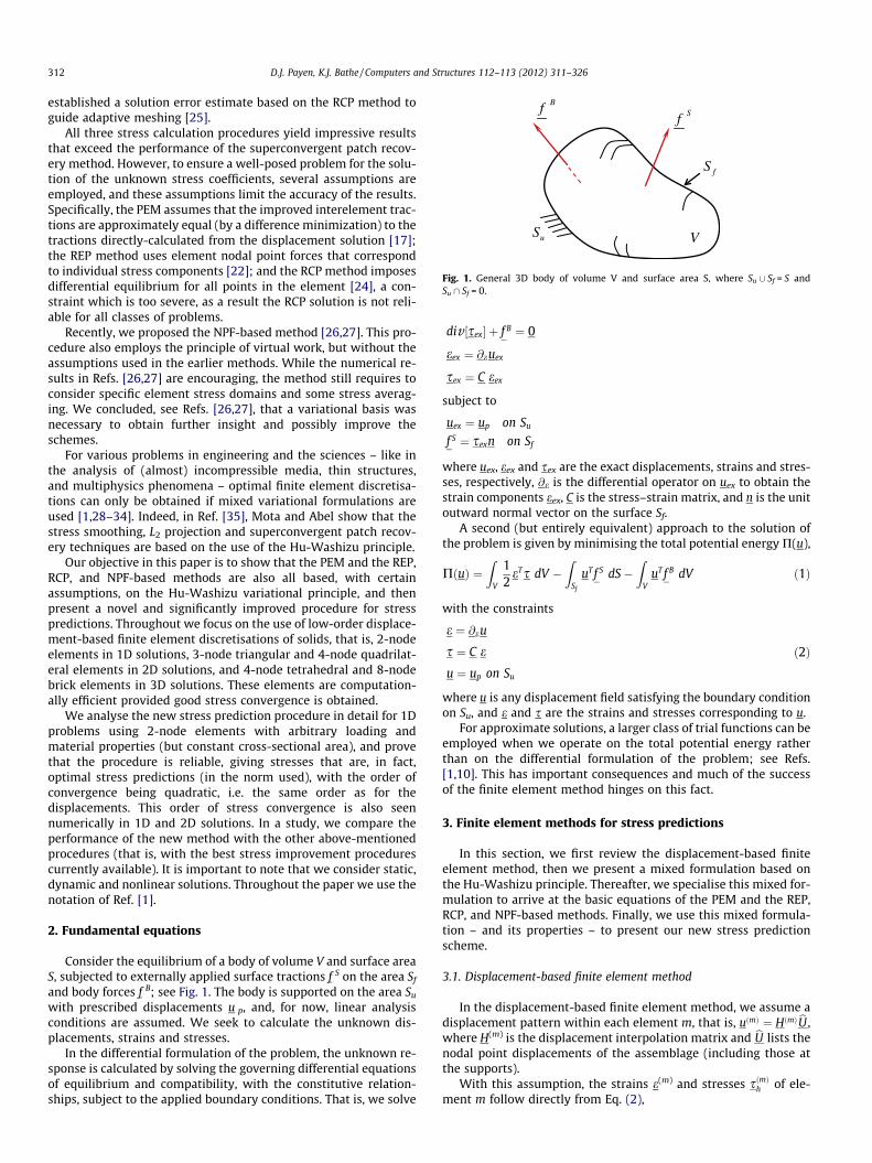
Fig. 1. General 3D body of volume V and surface area S, where Su [ Sf = S andSu \ Sf = 0.

312 D.J. Payen, K.J. Bathe / Computers and Structures 112–113 (2012) 311–326

established a solution error estimate based on the RCP method toguide adaptive meshing [25].

All three stress calculation procedures yield impressive resultsthat exceed the performance of the superconvergent patch recov-ery method. However, to ensure a well-posed problem for the solu-tion of the unknown stress coefficients, several assumptions areemployed, and these assumptions limit the accuracy of the results.Specifically, the PEM assumes that the improved interelement trac-tions are approximately equal (by a difference minimization) to thetractions directly-calculated from the displacement solution [17];the REP method uses element nodal point forces that correspondto individual stress components [22]; and the RCP method imposesdifferential equilibrium for all points in the element [24], a con-straint which is too severe, as a result the RCP solution is not reli-able for all classes of problems.

Recently, we proposed the NPF-based method [26,27]. This pro-cedure also employs the principle of virtual work, but without theassumptions used in the earlier methods. While the numerical re-sults in Refs. [26,27] are encouraging, the method still requires toconsider specific element stress domains and some stress averag-ing. We concluded, see Refs. [26,27], that a variational basis wasnecessary to obtain further insight and possibly improve theschemes.

For various problems in engineering and the sciences – like inthe analysis of (almost) incompressible media, thin structures,and multiphysics phenomena – optimal finite element discretisa-tions can only be obtained if mixed variational formulations areused [1,28–34]. Indeed, in Ref. [35], Mota and Abel show that thestress smoothing, L2 projection and superconvergent patch recov-ery techniques are based on the use of the Hu-Washizu principle.

Our objective in this paper is to show that the PEM and the REP,RCP, and NPF-based methods are also all based, with certainassumptions, on the Hu-Washizu variational principle, and thenpresent a novel and significantly improved procedure for stresspredictions. Throughout we focus on the use of low-order displace-ment-based finite element discretisations of solids, that is, 2-nodeelements in 1D solutions, 3-node triangular and 4-node quadrilat-eral elements in 2D solutions, and 4-node tetrahedral and 8-nodebrick elements in 3D solutions. These elements are computation-ally efficient provided good stress convergence is obtained.

We analyse the new stress prediction procedure in detail for 1Dproblems using 2-node elements with arbitrary loading andmaterial properties (but constant cross-sectional area), and provethat the procedure is reliable, giving stresses that are, in fact,optimal stress predictions (in the norm used), with the order ofconvergence being quadratic, i.e. the same order as for thedisplacements. This order of stress convergence is also seennumerically in 1D and 2D solutions. In a study, we compare theperformance of the new method with the other above-mentionedprocedures (that is, with the best stress improvement procedurescurrently available). It is important to note that we consider static,dynamic and nonlinear solutions. Throughout the paper we use thenotation of Ref. [1].

2. Fundamental equations

Consider the equilibrium of a body of volume V and surface areaS, subjected to externally applied surface tractions f S on the area Sf

and body forces f B; see Fig. 1. The body is supported on the area Su

with prescribed displacements u p, and, for now, linear analysisconditions are assumed. We seek to calculate the unknown dis-placements, strains and stresses.

In the differential formulation of the problem, the unknown re-sponse is calculated by solving the governing differential equationsof equilibrium and compatibility, with the constitutive relation-ships, subject to the applied boundary conditions. That is, we solve

div ½sex� þ f B ¼ 0

eex ¼ @euex

sex ¼ C eex

subject to

uex ¼ up on Su

f S ¼ sexn on Sf

where uex, eex and sex are the exact displacements, strains and stres-ses, respectively, @e is the differential operator on uex to obtain thestrain components eex, C is the stress–strain matrix, and n is the unitoutward normal vector on the surface Sf.

A second (but entirely equivalent) approach to the solution ofthe problem is given by minimising the total potential energy P(u),

PðuÞ ¼Z

V

12eTs dV �

ZSf

uT f S dS�Z

VuT f B dV ð1Þ

with the constraints

e ¼ @eu

s ¼ C e

u ¼ up on Su

ð2Þ

where u is any displacement field satisfying the boundary conditionon Su, and e and s are the strains and stresses corresponding to u.

For approximate solutions, a larger class of trial functions can beemployed when we operate on the total potential energy ratherthan on the differential formulation of the problem; see Refs.[1,10]. This has important consequences and much of the successof the finite element method hinges on this fact.

3. Finite element methods for stress predictions

In this section, we first review the displacement-based finiteelement method, then we present a mixed formulation based onthe Hu-Washizu principle. Thereafter, we specialise this mixed for-mulation to arrive at the basic equations of the PEM and the REP,RCP, and NPF-based methods. Finally, we use this mixed formula-tion – and its properties – to present our new stress predictionscheme.

3.1. Displacement-based finite element method

In the displacement-based finite element method, we assume adisplacement pattern within each element m, that is, uðmÞ ¼ HðmÞ bU ,where H(m) is the displacement interpolation matrix and bU lists thenodal point displacements of the assemblage (including those atthe supports).

With this assumption, the strains e(m) and stresses sðmÞh of ele-ment m follow directly from Eq. (2),

D.J. Payen, K.J. Bathe / Computers and Structures 112–113 (2012) 311–326 313

eðmÞ ¼ @euðmÞ ¼ BðmÞ bU ð3ÞsðmÞh ¼ CðmÞeðmÞ ¼ CðmÞBðmÞ bU ð4Þ

Then, minimising P of Eq. (1) yields

XN

m¼1

ZV ðmÞ

BðmÞT CðmÞBðmÞ dV� �" #bU

¼XN

m¼1

ZSðmÞ

f

HðmÞT f S dSþZ

V ðmÞHðmÞT f B dV

!( )ð5Þ

where B(m), C(m), V(m), and SðmÞf are the strain–displacement matrix,the stress–strain matrix, the volume, and the surface area withexternally applied tractions of element m, respectively. We sumover all N elements in the mesh and use Eq. (5) to obtain bU; seefor example Ref. [1]. Finally, sðmÞh is calculated using Eq. (4).

In the following, we focus on the use of low-order finite elementdiscretisations (the 2-node element in 1D solutions, the 3-nodeand 4-node elements in 2D solutions, etc.). It is well known thatthe accuracy of sðmÞh is then poor, as compared with the accuracyof the calculated displacements, and this deficiency can be seenusing stress band plots of unsmoothed stresses [1,8–10]. We referto these stresses as the ‘‘directly-calculated finite elementstresses’’.

3.2. Mixed formulation

To arrive at accurate stress predictions, a mixed interpolationapproach – which can be thought of as a special use of the Hu-Washizu principle – can be more effective. In this formulation,rather than applying the stress–strain relationship point-wise, werelax this relationship and apply it over the element volumes usingLagrange multipliers. The primary solution variables are then theunknown displacements, Lagrange multipliers and stresses. Hence,the equivalent of the minimisation of P in Eq. (1) is

P�ðuðmÞ;kðmÞ;sðmÞÞ ¼XN

m¼1

ZVðmÞ

12eðmÞTsðmÞ dV�

ZSðmÞ

f

uðmÞT f S dS

�Z

VðmÞuðmÞT f B dV�

ZV ðmÞ

kðmÞTfsðmÞ �CðmÞeðmÞg dV�

¼ stationary ð6Þ

with the constraints

eðmÞ ¼ @euðmÞ

uðmÞ ¼ up on Suð7Þ

As in the displacement-based finite element method, the dis-placements u(m) of element m are defined by nodal point variablesthat pertain to adjacent elements in the assemblage, uðmÞ ¼ HðmÞ bU ,and the strains e(m) follow directly from Eq. (7), eðmÞ ¼ BðmÞ bU . How-ever, the Lagrange multipliers k(m) and the stresses s(m) of elementm are defined by internal degrees of freedom that pertain only tothe specific element m considered.

In order to furnish improved stress predictions, we must as-sume a richer space for s(m) than that implicitly assumed for sðmÞh .Also, we want to enhance the fulfilment of equilibrium. Hence,we now assume

dimðsðmÞÞP dimðkðmÞÞP dimðeðmÞÞ ð8Þ

andZV ðmÞ

dfðmÞT div sðmÞ� �

þ f Bn o

dV ¼ 0 ð9Þ

where dim (.) denotes the dimension of the space of the variableconsidered, d denotes, as usual, ‘‘variation of’’, f(m) is an elementof a space discussed below (the space depends on the method used),

and the square parentheses indicate that the stress vector has beenarranged into matrix form.

With this assumption, invoking the stationarity of P⁄ with re-

spect to u(m), k(m) and s(m) yields

XN

m¼1

ZV ðmÞ

deðmÞT12sðmÞ þ CðmÞkðmÞ

� �dV

�

�Z

SðmÞf

duðmÞT f S dS�Z

V ðmÞduðmÞT f B dV

!¼ 0 ð10ÞZ

V ðmÞdkðmÞ TfsðmÞ � CðmÞeðmÞg dV ¼ 0 8 m ð11Þ

kðmÞ ¼ 12eðmÞ 8 m ð12Þ

Since Eq. (11) holds for all variations of k(m), including whendkðmÞ ¼ 1

2 deðmÞ, Eq. (10) contains as a special case

XN

m¼1

ZVðmÞ

deðmÞT12

CðmÞeðmÞ þ CðmÞkðmÞ� �

dV

�Z

SðmÞf

duðmÞT f S dS�Z

V ðmÞduðmÞT f B dV

!¼ 0

Then, using the solution kðmÞ ¼ 12 eðmÞ from Eq. (12) we obtain

XN

m¼1

ZVðmÞ

deðmÞT CðmÞeðmÞ dV�Z

SðmÞf

duðmÞT f S dS�Z

VðmÞduðmÞT f B dV

!¼0

ð13Þ

Of course, when inserting the element interpolations, Eq. (13)gives Eq. (5). Here Eq. (13) (and hence Eq. (5)) would give – at thisstage – a specific solution of the stresses in the stress space of s(m),namely sðmÞh . However, to complete the calculation of the improvedstresses we also use Eqs. (9) and (11).

An important practical feature of this ‘mixed formulation’ isthat the displacement problem in Eq. (13) is decoupled from theadditional calculations of the stresses. Therefore, in a general anal-

ysis, we first solve for u(m) as is standard, and then – rather than

applying the stress–strain relationship – we obtain s(m) from u(m)

by applying Eqs. (9) and (11) to each element m in the assemblage.This element-based approach works well in 1D solutions; how-

ever, in 2D and 3D solutions, better results are obtained when thestresses are defined over a predetermined patch of NP elements

known as the stress calculation domain. In this case, s(m) is ob-

tained from u(m) by applying Eqs. (9) and (11) either to each ele-ment m in the stress calculation domain, or to the entire stresscalculation domain,

XNP

m¼1

ZV ðmÞ

dkðmÞTfsðmÞ � CðmÞeðmÞgdV� �

¼ 0 ð14Þ

XNP

m¼1

ZV ðmÞ

dfðmÞTfdiv ½sðmÞ� þ f BgdV� �

¼ 0 ð15Þ

Since s(m) is obtained from u(m), the accuracy of s(m) is limited bythat of u(m); hence, the highest order of convergence of the stressesthat we can expect is O(h2) in the H0 norm (that is, in the L2 norm) –one order higher than that observed for sðmÞh .

The key question for the formulation is now: What interpola-

tions should be used for k(m) and f(m) to ensure a well-posed prob-lem with stresses that converge at order O(h2)? Indeed, the choiceof interpolation determines the number of equations available andthe accuracy of the results. Examples are given below.


3.3. The PEM and the REP method

In the PEM and the REP method, k(m) is interpolated in the sameway as the strains e(m) and f(m) is interpolated in the same way asthe displacements u(m). With this assumption, we obtain from Eqs.(14) and (15)

XNP

m¼1

ZV ðmÞ

deðmÞTsðmÞdV� �

¼XNP

m¼1

dbUTFðmÞ

� ð16Þ

XNP

m¼1

ZV ðmÞ

duðmÞT div ½sðmÞ� þ f Bn o

dV� �

¼ 0 ð17Þ

where dbU are the virtual nodal point displacements that correspondto de(m) and F(m) are the element nodal point forces, in fact alreadyused in Eq. (5),

FðmÞ ¼Z

V ðmÞBðmÞTsðmÞh dV ¼

ZV ðmÞ

BðmÞT CðmÞBðmÞdV �bU ð18Þ

Using the mathematical identity du(m)Tdiv[s(m)] = div(du(m)T

[s(m)]) � de(m)T s(m), the Gauss divergence theorem and Eq. (16),we can write Eq. (17) as

XNP

m¼1

ZSðmÞ

f

duðmÞT ½sðmÞ�nðmÞdSþZ

VðmÞduðmÞT f BdV

!¼XNP

m¼1

dbUTFðmÞ

� ð19Þ

where n(m) is the unit normal to the boundary surface SðmÞf of ele-ment m.

Eq. (19) is the basic equation of the PEM and Eq. (16) is the basicequation of the REP method. That is, for any virtual displacementpattern contained in the interpolation functions, the PEM balancesthe virtual work of the boundary tractions (adjusted for body forceeffects) with the virtual work of the nodal point forces, whereas theREP method balances the internal virtual work of the stresses withthe virtual work of the nodal point forces.

Since each method uses only one principle of virtual work state-ment (of the two possible statements given by the mixed formula-tion), the governing matrices corresponding to the basic equationsof the PEM and the REP method may be singular; hence, severalassumptions are employed to add extra constraints (and theseassumptions limit the accuracy of the results) – see Refs. [17,22].

3.4. The RCP method

Let Vs be the assumed stress space for s(m), and let �Vs be thesubspace of the self-equilibrated stresses in Vs. Then, let �sðmÞ beany element in that subspace

�Vs ¼ �sðmÞj �sðmÞ 2 Vs; div �sðmÞ� �

¼ 0�

ð20Þ

In the RCP method, k(m) is interpolated in the same way asCðmÞ�1�sðmÞ and f(m) is any element in L2(Vp), where L2(Vp) is the spaceof square integrable functions in the volume, Vp, of the stress calcu-lation domain. With this assumption, we obtain from Eqs. (14) and(15)

XNP

m¼1

ZV ðmÞ

d�sðmÞT CðmÞ�1sðmÞ � eðmÞ�

dV� �

¼ 0 ð21Þ

div ½sðmÞ� þ f B ¼ 0 ð22Þ

Eqs. (21) and (22) are basic equations of the RCP method. To sat-

isfy Eq. (22), an a priori particular solution sðmÞp:s: to the differential

equations of equilibrium is embedded in s(m) [23,24]. However,

establishing sðmÞp:s: for distorted isoparametric elements in dynamicanalysis is difficult and is an outstanding issue to be solved. More-

over, the differential equilibrium constraint in Eq. (22) is too se-vere, as a result the RCP solution is not reliable for all classes ofproblems; see section 5.

Considering nonlinear analysis, a complication with the RCPmethod is that the basic equations involve the use of the constitu-tive relationships; hence, in problems with path-dependent non-linear material conditions, an incremental solution proceduremay have to be used to solve for the unknown stress coefficientsin Eq. (21).

3.5. The NPF-based method

In the NPF-based method, k(m) is interpolated in the same wayas the strains e(m) and f(m) is interpolated in the same way as thedisplacements u(m). With this assumption we obtain from Eq.(11) and Eq. (9)Z

V ðmÞdeðmÞTsðmÞdV ¼ dbUT

FðmÞ ð23ÞZV ðmÞ

duðmÞTfdiv½sðmÞ� þ f BgdV ¼ 0 ð24Þ

where F(m) is defined in Eq. (18) and, using similar steps as thoseused to obtain Eq. (19), we can write Eq. (24) asZ

SðmÞf

duðmÞT ½sðmÞ�nðmÞdSþZ

VðmÞduðmÞT f BdV ¼ dbUT

FðmÞ ð25Þ

Eqs. (23) and (25) are the basic equations of the NPF-basedmethod. In contrast to the PEM and the REP method, the NPF-basedmethod uses both principle of virtual work statements, Eqs. (23)and (25), and applies them to each element m in the stress calcula-tion domain. Consequently, the problem solution for the unknownNPF-based stress coefficients is well-posed without the (limiting)assumptions used in the earlier methods.

However, a drawback of the NPF-based method is that the num-ber of equations available – and hence the dimension of the inter-polation functions assumed in Vs – is dependent on the number(and type) of elements in the stress calculation domain. Therefore,to get close to O(h2) convergence for the stresses, a large stress do-main is needed and a domain stress averaging procedure has beenemployed; see Refs. [26,27].

3.6. The new stress improvement procedure

In this section, we present a novel and significantly improvedprocedure for stress predictions. We first develop the method forlinear static and dynamic analysis and then we extend the methodto nonlinear solutions. Finally, we consider the computational costof the technique.

3.6.1. Linear static and dynamic analysisThe new stress improvement procedure assumes k(m) is interpo-

lated in the same way as the self-equilibrated stresses �sðmÞ and f(m)

is any element in P1(Vp), where Pk(Vp) is the space of completepolynomials of degree k in the volume, Vp, of the stress calculationdomain. With this assumption, we obtain from Eqs. (14) and (15)

XNP

m¼1

ZVðmÞ

d�sðmÞT sðmÞ � sðmÞh

n odV

� �¼ 0 ð26Þ

XNP

m¼1

ZVðmÞ

dfðmÞT div ½sðmÞ� þ f Bn o

dV� �

¼ 0 ð27Þ

where the stresses s(m) are assumed to be continuous and quadrat-ically interpolated across the stress calculation domain, s(m) 2 P2

(Vp), and the space of self-equilibrated stresses, �Vs, is given by

+ +− −

− −+ +

+ +− −

− −+ +

Fig. 2. Checkerboard mode of constant element stress. Here + and � denote þDsðmÞij

and �DsðmÞij , where DsðmÞij is an arbitrary value; see Ref. [1].


�Vs ¼ f�sðmÞj �sðmÞ 2 P2ðVpÞ; div ½�sðmÞ� ¼ 0g ð28Þ

Eqs. (26) and (27) are the basic equations used. The first equa-tion, Eq. (26), expresses that the projection of the difference in theenhanced and directly-calculated stresses onto �Vs shall be zero.Hence, this condition in essence extracts from sðmÞh that part whichis of good quality. The second equation, Eq. (27), then enforces thatthe difference in the divergence of the enhanced and the exactstresses in the projection onto the space P1 is also zero.

To obtain the corresponding finite element equations, we intro-duce the interpolations

sðmÞ ¼ Ess; �sðmÞ ¼ Es �s; fðmÞ ¼ Eff ð29Þ

where the interpolation matrices Es, Es, and Ef are given in Eq. (35)for 1D analysis, and in Eqs. (45)–(47), respectively, for 2D analysis.Note that in these matrices locally based coordinate origins are usedto avoid ill-conditioning, and div½Es� ¼ 0, as is required by Eq. (28).

Substituting from Eq. (29) into Eqs. (26) and (27) we arrive at

XNP

m¼1

RV ðmÞ ET

s EsdVRV ðmÞ ET

f @sEsdV

!" #s ¼

XNP

m¼1

RVðmÞ ET

s sðmÞh dV�R

VðmÞ ETf f BdV

!( )ð30Þ

where @s is the differential operator on s(m) to obtain the divergenceof the stress field (see Eqs. (36) and (48)), s lists the unknown stresscoefficients to be found, and, in dynamic analysis, we must includethe d’Alembert inertia forces in f B; see section 5.5.

Since s(m) 2 P2(Vp), and �sðmÞ 2 �Vs, f(m) 2 P1(Vp), it follows that Eq.(30) represents a determined system of equations in terms of s –irrespective of the number (and type) of elements used in the stresscalculation domain – such that a unique solution for s always ex-ists, even if only one element is used in the stress calculationdomain.

To summarise, the important attributes of the new method are:

1. The assumed stresses s(m) are interpolated with complete poly-nomials of degree 2; hence, the order of convergence of s(m) isexpected to be O(h2).

2. The number of equations available is independent of the num-ber (and type) of elements used in the stress calculationdomain.

3. The system of equations is always determined.4. The equations do not involve the use of the constitutive rela-

tionships (other than in the calculation of sðmÞh ).5. The stress calculations can be performed for the entire assem-

blage, or just in localised regions of concern.6. The fulfilment of differential equilibrium is enhanced, and dif-

ferential equilibrium is fulfilled at every point in the elementif f B 2 P1.

7. The method does not use an a priori particular solution (likeused in the RCP method).

8. sðmÞh can also be established from a mixed formulation (such asthe u/p formulation, the incompatible modes formulation, etc.),and the method can still be used to enhance the stress solution.

9. The enhanced stress solution will not be afflicted with a spuri-ous checkerboard mode of constant element stresses.

Spurious checkerboard modes of constant element stresses canbe found in some displacement-stress solutions – see Fig. 2 andRef. [1]. To prove that the improved stresses s(m) are not afflictedwe use Eq. (26) to obtain

XNP

m¼1

ZV ðmÞ

sðmÞdV� �

¼XNP

m¼1

ZV ðmÞ

sðmÞh dV� �

ð31Þ

and note that the directly-calculated stresses, sðmÞh , established in aproper formulation (e.g. the displacement formulation), are notafflicted.

Also, because the exact stresses satisfy the differential equa-tions of equilibrium, we can write Eq. (27) as

XNP

m¼1

ZV ðmÞ

dfðmÞT div½sðmÞ�dV� �

¼XNP

m¼1

ZV ðmÞ

dfðmÞT div½sex�dV� �

ð32Þ

such that

XNP

m¼1

ZV ðmÞ

div ½sðmÞ�dV� �

¼XNP

m¼1

ZV ðmÞ

div½sex�dV� �

ð33Þ

Eqs. (32) and (33) are important since they relate the calculatedand exact stresses in the volume of the stress calculation domain.Indeed, we shall use these relationships when we consider an errorbound on s(m).

Finally, we note that the PEM, and the REP and NPF-basedmethods satisfy the condition on k(m) given in Eq. (8), irrespectiveof NP. However, the RCP method and the new method only satisfythis condition when NP = 1 (because these two methods assumek(m) to be continuous across element boundaries whereas e(m) doesnot show that continuity).

3.6.2. Nonlinear analysisIn nonlinear analyses, all theory presented is applicable, but of

course the current volumes and current Cauchy stresses must beused; see Ref. [1]. That is, if t denotes ‘‘in the current configura-tion’’, the stress coefficients t s are obtained using

XNP

m¼1

Rt VðmÞ ET

s EsdVRt VðmÞ ET

f @sEsdV

!" #ts ¼

XNP

m¼1

Rt V ðmÞ ET

stsðmÞh dV

�R

t V ðmÞ ETf

tf BdV

!( )ð34Þ

where tVm is the current volume of element m (obtained from thedisplacement solution t bU), tsðmÞh lists the directly-calculated Cauchystresses at time t, and t bU is established using a step-by-step incre-mental solution procedure [1].

Therefore, once t bU has been established, the enhanced stresspredictions are obtained using Eq. (34), as in linear analysis.

3.6.3. Computational expenseThe computational expense to furnish improved stress predic-

tions is given by the numerical effort involved in solving for 18 un-known stress coefficients in 2D solutions (and the 60 unknownstress coefficients in 3D solutions) for each element m where stres-ses are to be improved.

This expense is small, compared with factorising the globalstiffness matrix. Indeed, the expense to enhance the stresses forthe entire assemblage in a typical linear static analysis problem(with 105 to 106 degrees of freedom) is probably only about 1%of the total solution cost. In nonlinear analyses the expense is, rel-

(a)

(b)Fig. 3. Ad-hoc test problem to assess the performance of the proposed scheme in1D solutions (E = 110 � 109, A = 1 � 10�4): (a) the test problem and (b) stressconvergence curves measured in the Sobolev norm k � kk of order k.

Fig. 4. Stress solutions to the 1D problem defined in Fig. 3a for various differentdensities of mesh, where N denotes the number of elements used.


atively, even lower because a step-by-step solution procedure isneeded to obtain t bU .

Of course, in practice, the stress calculations need not be per-formed for the entire assemblage, but instead might be performedonly for those elements where stresses should be improved.

4. Insight into the new procedure in 1D solutions

In this section, we first present the solution procedure of thenew stress improvement method in 1D settings, then we analysethe method in detail. Thereafter, we compare the performance ofthe new method with that of the PEM and the REP method.

4.1. Matrices used in 1D solutions

In the following, we consider the 1D case with only one stresscomponent, for arbitrary loading and material properties, and as-sume that the cross-sectional area of the 1D structure is constant.In this case, an element-based approach is adopted. Hence, to solve

for the unknown stress coefficients s for a general element m, weapply Eq. (30) with NP = 1,

Es ¼ 1 x x2� �

; Es ¼ ½1�; Ef ¼ 1 x½ � ð35Þ

and

@s ¼ddx

�ð36Þ

where s ¼ a1 a2 a3f gT , and x is the element m local coordinatesystem.

4.2. Reliability, optimality and convergence of the stress prediction

The fundamental objective of the new procedure is to enhancethe accuracy of the stresses. Mathematically, therefore, our goalis to find stresses s(m) such that

XN

m¼1

ksex � sðmÞkV ðmÞ 6 cXN

m¼1

sex � sðmÞh

�� VðmÞ

ð37Þ

with a constant c < 1, dependent on the problem, and ideally c <<1.Here we use the H1 semi-norm k � kVðmÞ which, when the function

in the norm is zero on some part of the boundary, is equivalent tothe H1 norm (by the Poincaré–Friedrichs inequality [1,28]). Thesemi-norm is appropriate for the stresses because of Eq. (31). Weanalyse the 1D case considered in Section 4.1 and give details toprovide some insight.

In this case, the distance between the exact and the calculatedsolution is

ksex � sðmÞk2V ðmÞ ¼ ksexk2

VðmÞ þ ksðmÞk2

V ðmÞ

� 2Z

VðmÞ

dsðmÞ

dx

� �dsex

dx

� �dV

� �ð38Þ

Because NP = 1, Eq. (32) gives

Fig. 5. Stress convergence curves measured in the Sobolev norm k � kk of order k tothe 1D problem defined in Fig. 3a, where, in this case, the Young’s modulus varies asE = 110(1 + 0.64sin (20px)) � 109.

Fig. 6. Rotor blade problem (E = 110 � 109, q = 4400, and x = 10). The rotor bladespins at a sufficiently high rate that gravitational forces are negligible as comparedwith the centrifugal forces which act on the blade. The blade is either pinned atnode 1 and is free at node 3 (bU1 ¼ 0 and bU3 – 0), or is pinned at node 1 and iswelded to a rigid hoop at node 3 ðbU1 ¼ bU3 ¼ 0Þ.

(a)

(b)

Fig. 7. Stress results for the rotor blade problem defined in Fig. 6: (a) the staticallydeterminate pinned-free case (bU1 ¼ 0 and bU3 – 0) and (b) the statically indeter-minate pinned–pinned case ðbU1 ¼ bU3 ¼ 0Þ.


ZV ðmÞ

dfðmÞdsex

dx

� �dV ¼

ZV ðmÞ

dfðmÞdsðmÞ

dx

� �dV

for all variations of f(m) 2 P1, including when dfðmÞ ¼ dsðmÞdx

� .

ThereforeZV ðmÞ

dsðmÞ

dx

� �dsex

dx

� �dV ¼ ksðmÞk2

V ðmÞ

and hence we obtain from Eq. (38) the result

ksex � sðmÞk2V ðmÞ ¼ ksexk2

V ðmÞ � ksðmÞk2

VðmÞ ð39Þ

Using the Cauchy–Schwarz inequality [1,28]

ksðmÞk2VðmÞ P

1V ðmÞ

ZV ðmÞ

dsðmÞ

dx

� �dV

� �2

and the propertyR

V ðmÞdsðmÞ

dx

� dV ¼

RV ðmÞ

dsexdx

� �dV , which follows from

Eq. (33), we have

ksðmÞk2V ðmÞ P

1V ðmÞ

ZV ðmÞ

dsex

dx

� �dV

� �2

¼ 1V ðmÞ

RV ðmÞ

dsexdx

� �dV

� �2RV ðmÞ

dsexdx

� �2dVksexk2

VðmÞ ð40Þ

In light of Eqs. (39) and (40), we obtain

ksex � sðmÞk2V ðmÞ 6 1� 1

V ðmÞ

RVðmÞ

dsexdx

� �dV

� �2RVðmÞ

dsexdx

� �2dV

!ksexk2

VðmÞ ð41Þ

Finally, because the displacements vary linearly, then

sex � sðmÞh

�� 2

V ðmÞ¼ ksexk2

V ðmÞ

and hence we obtain from Eq. (41) the required result

ksex � sðmÞkV ðmÞ 6 c sex � sðmÞh

�� VðmÞ

ð42Þ

with

c ¼ 1� 1V ðmÞ

RV ðmÞ

dsexdx

� �dV

� �2RV ðmÞ

dsexdx

� �2dV

!12

where c < 1. It is interesting to note that if sex 2 P1, we have c = 0,such that the calculated stresses are exact (when measured in theH1 semi-norm), irrespective of the coarseness of mesh used.

(a)

(b)

Fig. 8. Stress results for the rotor blade problem defined in Fig. 6: (a) the staticallydeterminate pinned-free case (bU1 ¼ 0 and bU3 – 0) and (b) the statically indeter-minate pinned–pinned case ðbU1 ¼ bU3 ¼ 0Þ. The PEM assumes a linear stress, theREP method assumes a constant stress, and the proposed scheme assumes aquadratic stress in each element domain.

Fig. 9. Stress calculation domain used to solve for the unknown stress coefficients sfor a general 2D 4-node element m.

Fig. 10. Stress calculation domain used to solve for the unknown stress coefficientss at a specific node i for a 2D 4-node element mesh.

Fig. 11. Stress calculation domain for a general 2D 4-node element m between atitanium housing and a steel Keensert. Element m belongs to the titanium housinggroup of elements. Since the steel Keensert elements are not included in the stressdomain, there is no smoothing across the material discontinuity.


Eq. (42) proves the new method satisfies the fundamentalrequirement in Eq. (37) for each element, as well as for the entiredomain. Also, because sðmÞh is stable and converging in the norm[1,10], Eq. (42) proves the method is reliable in 1D solutions andthe stresses (within each element) are always more accurate thansðmÞh when measured in the norm used.

Furthermore, it can be proved (following the usual procedures[1]) that the new method chooses s(m) so as to minimise the errorwithin the volume of each element m, i.e. s(m) is, in fact, the optimalstress prediction,

ksex � sðmÞkV ðmÞ 6 ksex � ~sðmÞkVðmÞ 8~sðmÞ 2 P2 ð43Þ

and using interpolation theory on s(m) with the result given in Eq.(43), it can also be proved that

XN

m¼1

ksex � sðmÞkV ðmÞ 6 ch2 ð44Þ

where the constant c is independent of h, but depends on the exactsolution sex.

Therefore, s(m) converges to the exact theory of elasticity solu-tion with order O(h2) in the H1 norm. In problems where the nodalpoint displacements are the exact displacements (e.g in Fig. 3), weindeed observed that s(m) converges at O(h3) in the H0 norm. How-ever, if the nodal point displacements are not the exact displace-ments, the accuracy of s(m) is limited by that of u(m); hence, the

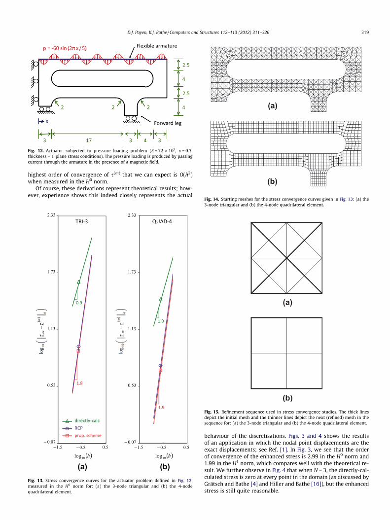
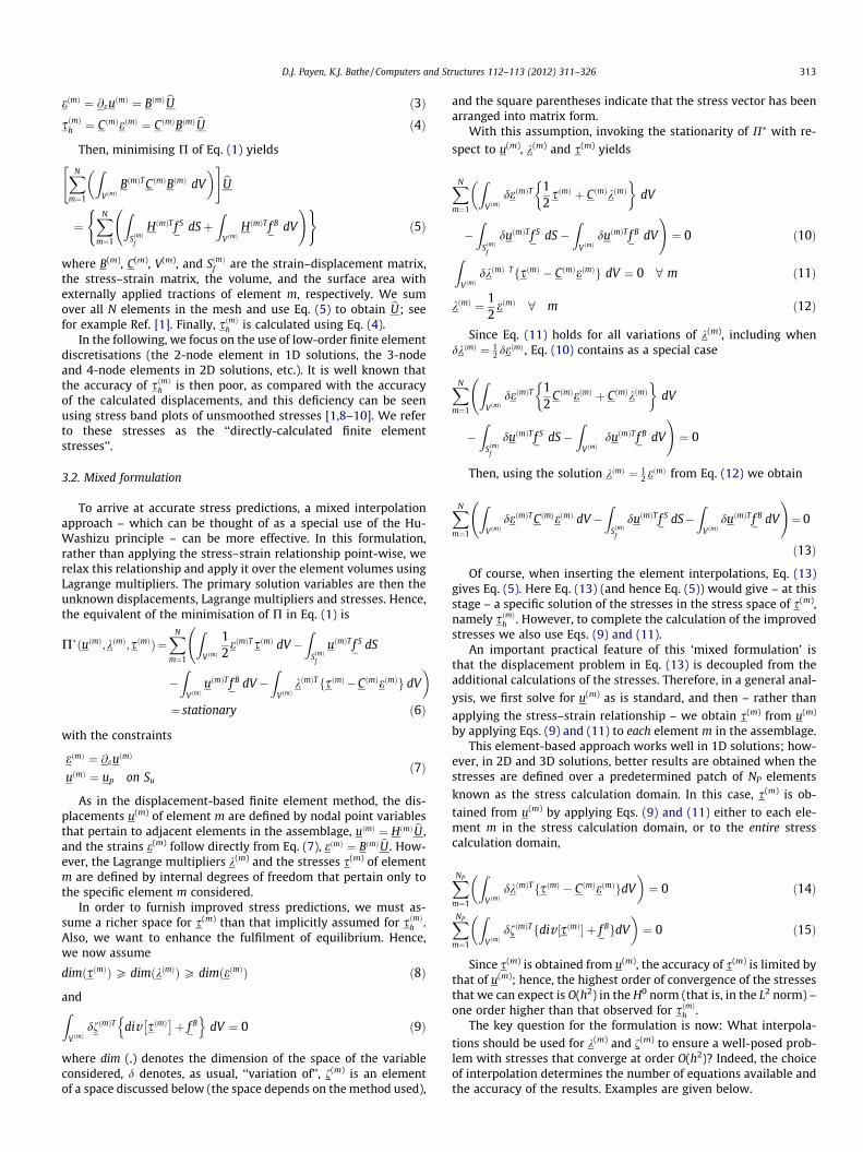
Fig. 12. Actuator subjected to pressure loading problem (E = 72 � 103, t = 0.3,thickness = 1, plane stress conditions). The pressure loading is produced by passingcurrent through the armature in the presence of a magnetic field.

(a)

(b)

Fig. 14. Starting meshes for the stress convergence curves given in Fig. 13: (a) the


highest order of convergence of s(m) that we can expect is O(h2)when measured in the H0 norm.

Of course, these derivations represent theoretical results; how-ever, experience shows this indeed closely represents the actual

(a) (b)Fig. 13. Stress convergence curves for the actuator problem defined in Fig. 12,measured in the H0 norm for: (a) the 3-node triangular and (b) the 4-nodequadrilateral element.

3-node triangular and (b) the 4-node quadrilateral element.

(a)

(b)Fig. 15. Refinement sequence used in stress convergence studies. The thick linesdepict the initial mesh and the thinner lines depict the next (refined) mesh in thesequence for: (a) the 3-node triangular and (b) the 4-node quadrilateral element.

behaviour of the discretisations. Figs. 3 and 4 shows the resultsof an application in which the nodal point displacements are theexact displacements; see Ref. [1]. In Fig. 3, we see that the orderof convergence of the enhanced stress is 2.99 in the H0 norm and1.99 in the H1 norm, which compares well with the theoretical re-sult. We further observe in Fig. 4 that when N = 3, the directly-cal-culated stress is zero at every point in the domain (as discussed byGrätsch and Bathe [4] and Hiller and Bathe [16]), but the enhancedstress is still quite reasonable.


Fig. 5 shows the results of an application in which the nodalpoint displacements are not the exact displacements. As expected,in this case, s(m) converges at O(h2) in the H0 norm, the same as foru(m), but one order higher than that observed for sðmÞh .

4.3. Numerical example: a rotor blade problem

To illustrate the effectiveness of the new procedure, the re-sponse of a rotor blade is studied. Fig. 6 defines the problem. Theinboard end of the rotor blade is driven at a constant angular veloc-ity x; the outboard end is either left free or is welded to a rigidhoop. The rotor blade is idealised as an assemblage of two 2-nodetruss elements, and the problem is solved using both the usual dis-placement-based method and the proposed scheme.

We note that in this problem one element has a constant cross-sectional area whereby the other element has a varying area, asshown in Fig. 6. The varying area enters in the equilibrium equa-tion, so that Eq. (15) becomesZ

LðmÞdfðmÞT

ddxðAðxÞsðmÞÞ þ AðxÞf B

x

� �dx ¼ 0

where L(m) and A(x) are the length and cross-sectional area of ele-ment m, respectively, and the area is a function of x.

Fig. 7 shows the stress results. In Fig. 7 (and in all other figures),‘‘exact’’ refers to the exact analytical (or a very accurate numerical)

Fig. 16. Stress convergence curves for the actuator problem defined in Fig. 12,measured in the H0 norm, for the 4-node quadrilateral element with (dashed line)and without incompatible modes (solid line).

solution of the mathematical model, ‘‘directly-calc’’ refers to thedirectly-calculated finite element stresses, and ‘‘prop. scheme’’ re-fers to the finite element stresses predicted using the proposedstress improvement scheme.

Considering the results, we see that the enhanced solution forthe stress is significantly more accurate than given directly bythe displacements. We further observe that the gradient of the en-hanced stress is exact at every point in element 1. Indeed, this willalways be the case when the exact stress varies quadraticallyacross the element domain; see Eq. (43).

Next, the rotor blade problem is solved using the PEM [17] andthe improved REP method [22]. Typically, the PEM is used to calcu-late improved interelement tractions for the purposes of error esti-mation; however, in our comparison the governing equations ofthe PEM are used to calculate improved stresses.

Fig. 8 shows the stress results, where, for consistency, all meth-ods use only one element in the stress calculation domain. We seethat the new procedure performs best. This is expected because thenew procedure uses a stress with a higher degree of interpolationthan can be used with the other methods, and (most importantly)the solution of the new procedure satisfies the properties discussedin Section 3.6.1. Also, the assumptions employed in the PEM andthe REP method limit the accuracy of the results; see Refs.[17,22] and the earlier discussion in Section 1.

Lastly, we note that when f B 2 P1, the solution obtained usingthe RCP method is similar to that obtained using the new method(see Section 5.4.1); hence, for clarity, we do not consider the RCPresults here.

5. Insight into the new procedure in 2D solutions

In this section, we first present the solution procedure of thenew stress improvement method in 2D settings for a general ele-ment m. Then, we discuss how to establish enhanced stresses ata specific node i and how to deal with discontinuous solutions.Thereafter, we assess the performance of the method in static, dy-namic and nonlinear solutions.

Since the performance of the RCP methods exceeds that of theREP method (by a considerable margin) [23], we only comparethe stresses of the new procedure with the RCP stresses here.

5.1. Matrices used in 2D solutions

In 2D (and 3D) problems, better results are obtained when mul-tiple elements are used in the stress calculation domain. Hence, tosolve for the unknown stress coefficients s for a general element m,we use the union of elements that surrounds (and includes) ele-ment m as the stress calculation domain; see Fig. 9. Then, we applyEq. (30) with

ð45Þ

ð46Þ

ð47Þ

and

Fig. 17. von Mises stress band plots for the actuator problem defined in Fig. 12, where the forward leg rollers are removed and the material stiffness is reduced by a factor 10.The plate is idealised as an assemblage of 3-node triangular elements. The stress in the band plots is un-averaged (and is shown on the deformed geometry), while thenumerical stress values are the averaged nodal point stresses, with the solution error given in parentheses.

Fig. 18. Large displacement, large strain, rubber plate problem, stretched to 100% ofits original length (Ogden material law: l1 = 0.7, l2 = �0.3, l3 = 0.01, a1 = 1.8,a2 = �1.6, a3 = 7.5, j = 1000, thickness = 0.5, plane stress conditions). Because ofsymmetry, only one-quarter of the plate is modelled.


@s ¼@@y 0 @

@z

0 @@z

@@y

" #ð48Þ

where and (y, z)are the locally based coordinates of the stress calculation domain.

The above description completely defines the stress calculationdomain for all types of element and mesh patterns, and no specialprocedures are needed near the boundaries (nor at the corners) ofthe mesh. Also, because there is only one possible configuration ofstress domain for each element m, the averaging procedure re-quired in Refs. [26,27] is no longer needed.

The RCP method uses the same definition of stress calculationdomain [24].

5.2. Solution procedure for a specific node i

For certain problems, we are interested in the stresses at a spe-cific node i, rather than within the element domain. In this situa-tion, we use the union of elements connected to node i as thestress calculation domain. Then, we apply Eq. (30) to solve forthe unknown stress coefficients, with the interpolation matrices gi-ven in Eqs. (45)–(47).

In the exceptional case where only one element m is connectedto node i (e.g. in a corner of the meshed geometry), the elementsproperly connected to element m should also be included in thestress domain; see Fig. 10.

5.3. Dealing with discontinuous solutions

In an actual implementation, the stress calculation domain onlycontains elements with equal settings. Boundaries between theelement groups are treated as free boundaries; see for example

Fig. 19. von Mises stress band plots to the rubber plate problem defined in Fig. 18.The plate is idealised as an assemblage of 3-node triangular elements and theresults are shown in the same format as in Fig. 17.

Fig. 20. von Mises stress results along section A–A to the rubber plate problemdefined in Fig. 18. The coordinate z references the deformed geometry.


Fig. 11. This prevents the scheme from smoothing discontinuitiespresent in the exact solution.

5.4. Static analysis problems

Two classes of problems are considered: the first where f B 2 P1

and the second where f B R P1. We show that the new stressimprovement method gives good results for both classes ofproblems, whereas the RCP method only performs well whenf B 2 P1.

5.4.1. The actuator problem: a case when f B 2 P1

The first problem solution involves an actuator subjected topressure loading. Fig. 12 defines the problem. The problem is stat-ically indeterminate and is solved using both the new method andthe RCP method.

Fig. 13 shows the stress convergence curves when a sequence of3- and 4-node element meshes are used for the solutions. The se-quence of meshes is constructed by starting with a mesh of uni-form elements of (approximately) equal size, see Fig. 14, then

subdividing each element into four equal new elements to obtainthe next (refined) mesh in the sequence and so on; see Fig. 15.The mesh size parameter h is calculated by averaging the size ofall elements in the assemblage (where the size is taken to be thediameter of a circle which encompasses that element).

Considering the results in Fig. 13, we see that the RCP solution issimilar to the solution obtained using the proposed scheme. Thiswill always be the case when f B 2 P1 because the quadraticallyvarying stresses are sufficiently rich to satisfy equilibrium for allpoints in the stress calculation domain; that is, Eq. (27) reducesto Eq. (22) when f B 2 P1. However, the solutions are not identicaldue to the Poisson coupling effects in Eq. (21).

The new procedure can also be used to furnish improved stresspredictions for the incompatible modes formulation [1]; seeFig. 16. In these calculations, the unknown stress coefficients areobtained using Eq. (30), where sðmÞh is established from the incom-patible modes solution. This enriches the space implicitly assumedfor sðmÞh , but since s(m) is still assumed to be quadratically interpo-lated, the solution for s(m) is similar both with and without incom-patible modes.

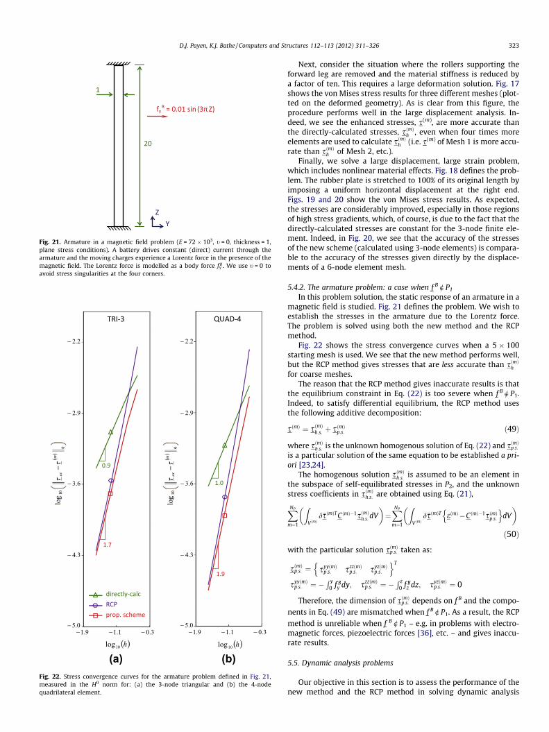
Fig. 21. Armature in a magnetic field problem (E = 72 � 103, t = 0, thickness = 1,plane stress conditions). A battery drives constant (direct) current through thearmature and the moving charges experience a Lorentz force in the presence of themagnetic field. The Lorentz force is modelled as a body force f B

Y . We use t = 0 toavoid stress singularities at the four corners.

directly-calc

RCP

prop. scheme

0.9

1.7

1.0

1.9

Fig. 22. Stress convergence curves for the armature problem defined in Fig. 21,measured in the H0 norm for: (a) the 3-node triangular and (b) the 4-nodequadrilateral element.


Next, consider the situation where the rollers supporting theforward leg are removed and the material stiffness is reduced bya factor of ten. This requires a large deformation solution. Fig. 17shows the von Mises stress results for three different meshes (plot-ted on the deformed geometry). As is clear from this figure, theprocedure performs well in the large displacement analysis. In-deed, we see the enhanced stresses, s(m), are more accurate thanthe directly-calculated stresses, sðmÞh , even when four times moreelements are used to calculate sðmÞh (i.e. s(m) of Mesh 1 is more accu-rate than sðmÞh of Mesh 2, etc.).

Finally, we solve a large displacement, large strain problem,which includes nonlinear material effects. Fig. 18 defines the prob-lem. The rubber plate is stretched to 100% of its original length byimposing a uniform horizontal displacement at the right end.Figs. 19 and 20 show the von Mises stress results. As expected,the stresses are considerably improved, especially in those regionsof high stress gradients, which, of course, is due to the fact that thedirectly-calculated stresses are constant for the 3-node finite ele-ment. Indeed, in Fig. 20, we see that the accuracy of the stressesof the new scheme (calculated using 3-node elements) is compara-ble to the accuracy of the stresses given directly by the displace-ments of a 6-node element mesh.

5.4.2. The armature problem: a case when f B R P1

In this problem solution, the static response of an armature in amagnetic field is studied. Fig. 21 defines the problem. We wish toestablish the stresses in the armature due to the Lorentz force.The problem is solved using both the new method and the RCPmethod.

Fig. 22 shows the stress convergence curves when a 5 � 100starting mesh is used. We see that the new method performs well,but the RCP method gives stresses that are less accurate than sðmÞh

for coarse meshes.The reason that the RCP method gives inaccurate results is that

the equilibrium constraint in Eq. (22) is too severe when f B R P1.Indeed, to satisfy differential equilibrium, the RCP method usesthe following additive decomposition:

sðmÞ ¼ sðmÞh:s: þ sðmÞp:s: ð49Þ

where sðmÞh:s: is the unknown homogenous solution of Eq. (22) and sðmÞp:s:

is a particular solution of the same equation to be established a pri-ori [23,24].

The homogenous solution sðmÞh:s: is assumed to be an element inthe subspace of self-equilibrated stresses in P2, and the unknownstress coefficients in sðmÞh:s: are obtained using Eq. (21),

XNP

m¼1

ZV ðmÞ

d�sðmÞT CðmÞ�1sðmÞh:s:dV� �

¼XNP

m¼1

ZV ðmÞ

d�sðmÞT eðmÞ �CðmÞ�1sðmÞp:s:

n odV

� �ð50Þ

with the particular solution sðmÞp:s: taken as:

sðmÞp:s: ¼ syyðmÞp:s: szzðmÞ

p:s: syzðmÞp:s:

n oT

syyðmÞp:s: ¼ �

R y0 f B

y dy; szzðmÞp:s: ¼ �

R z0 f B

z dz; syzðmÞp:s: ¼ 0

Therefore, the dimension of sðmÞp:s: depends on f B and the compo-

nents in Eq. (49) are mismatched when f B R P1. As a result, the RCP

method is unreliable when f B R P1 – e.g. in problems with electro-magnetic forces, piezoelectric forces [36], etc. – and gives inaccu-rate results.

5.5. Dynamic analysis problems

Our objective in this section is to assess the performance of thenew method and the RCP method in solving dynamic analysis

Fig. 23. Impact of an elastic bar (E = 200 � 109, q = 8000, A = 1). The bar is initiallyat rest and the response at time t = 1 � 10�3 is sought. During this time the wavepropagates to x = 5, there are no reflections. The bar is idealised as an assemblage of1D 2-node elements of size h = 0.025 (400 elements). We give the best resultsobtained using the Newmark method and the Bathe method when changing foreach method the time step size (i.e. the CFL number).

Fig. 24. Propagation of a wave in an elastic bar problem (E = 200 � 109, q = 8000,t = 0, thickness = 0.2, plane stress conditions). The bar is initially at rest and issubjected to a sudden pressure load at one end. The response at timet = 1.3 � 10�3 is sought. During this time the wave propagates to x = 6.5, thereare no reflections.

Fig. 25. Longitudinal stress results at t = 1.3 � 10�3 to the wave propagationproblem defined in Fig. 24. The bar is idealised as an assemblage of regular 4-nodequadrilateral elements, where h denotes the element size and Dt is the time stepused. In each case, CFL number = 1.

Fig. 26. Lightweight cantilevered plate subjected to base excitation problem(E = 200 � 109, q = 7800, t = 0, thickness = 1, plane stress conditions). The plate isinitially at rest and the response at t = 0.01902 is sought. No physical damping isintroduced in the model. The base of the plate is rigid and the enforceddisplacement dynamically excites the first eight natural modes of the plate. Weuse t = 0 to avoid stress singularities at the two corners of the built-in end.


problems. We show that the new method performs well in dy-namic analysis and can be used for distorted isoparametric ele-ments, whereas the RCP method can only be used if the elementsin the assemblage are un-distorted.

5.5.1. Solution procedureStress calculations in dynamics are performed as those in stat-

ics, except now the d’Alembert inertia forces are included in f B.That is, to obtain the stress coefficients t s of the new method attime t, we use

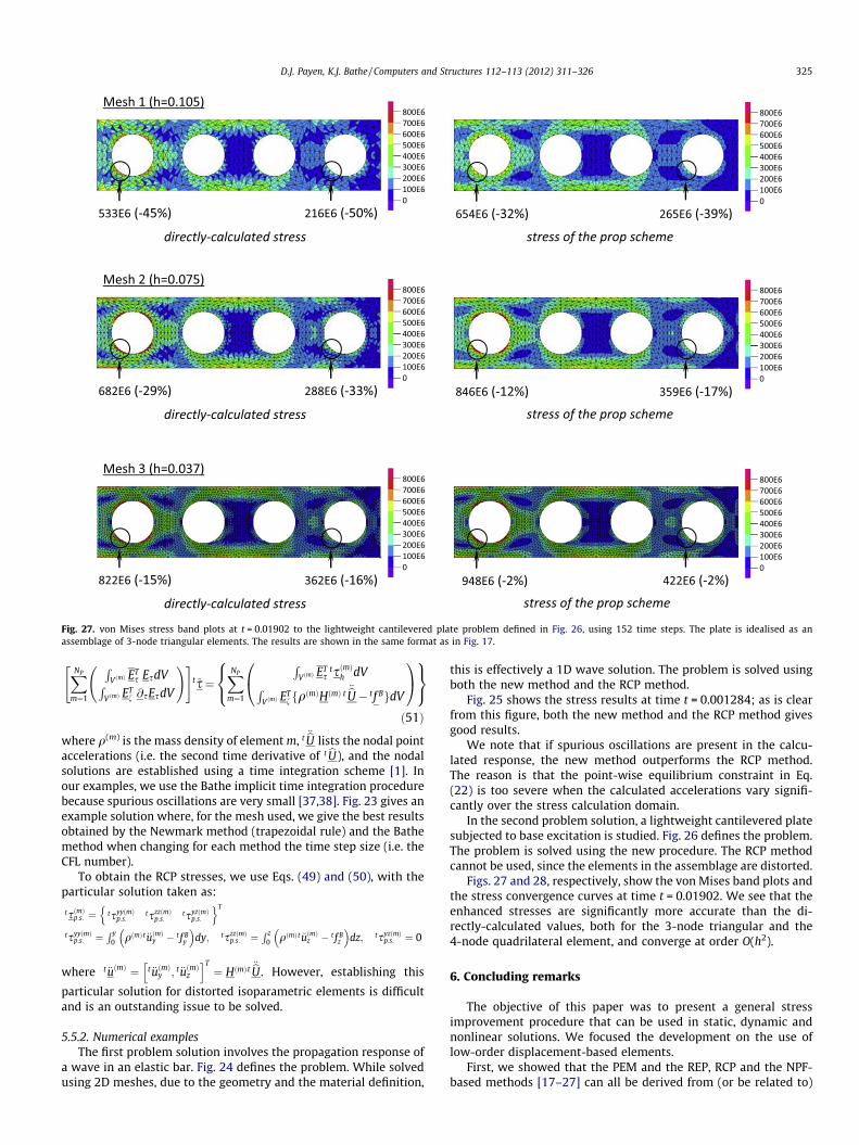
Fig. 27. von Mises stress band plots at t = 0.01902 to the lightweight cantilevered plate problem defined in Fig. 26, using 152 time steps. The plate is idealised as anassemblage of 3-node triangular elements. The results are shown in the same format as in Fig. 17.


XNP

m¼1

RVðmÞ E

Ts EsdVR

V ðmÞ ETf @sEsdV

!" #t s¼

XNP

m¼1

RV ðmÞ E

Ts

tsðmÞh dVRV ðmÞ E

Tf fqðmÞHðmÞ t €bU � tf BgdV

0@ 1A8<:9=;

ð51Þ

where q(m) is the mass density of element m, t €bU lists the nodal pointaccelerations (i.e. the second time derivative of t bU), and the nodalsolutions are established using a time integration scheme [1]. Inour examples, we use the Bathe implicit time integration procedurebecause spurious oscillations are very small [37,38]. Fig. 23 gives anexample solution where, for the mesh used, we give the best resultsobtained by the Newmark method (trapezoidal rule) and the Bathemethod when changing for each method the time step size (i.e. theCFL number).

To obtain the RCP stresses, we use Eqs. (49) and (50), with theparticular solution taken as:

tsðmÞp:s: ¼ tsyyðmÞp:s:

tszzðmÞp:s:

tsyzðmÞp:s:

n oT

tsyyðmÞp:s: ¼

R y0 qðmÞt €uðmÞy � t f B

y

� dy; tszzðmÞ

p:s: ¼R z

0 qðmÞ t €uðmÞz � t f Bz

� dz; tsyzðmÞ

p:s: ¼ 0

where t €uðmÞ ¼ t €uðmÞy ; t €uðmÞz

h iT¼ HðmÞt

€bU . However, establishing this

particular solution for distorted isoparametric elements is difficultand is an outstanding issue to be solved.

5.5.2. Numerical examplesThe first problem solution involves the propagation response of

a wave in an elastic bar. Fig. 24 defines the problem. While solvedusing 2D meshes, due to the geometry and the material definition,

this is effectively a 1D wave solution. The problem is solved usingboth the new method and the RCP method.

Fig. 25 shows the stress results at time t = 0.001284; as is clearfrom this figure, both the new method and the RCP method givesgood results.

We note that if spurious oscillations are present in the calcu-lated response, the new method outperforms the RCP method.The reason is that the point-wise equilibrium constraint in Eq.(22) is too severe when the calculated accelerations vary signifi-cantly over the stress calculation domain.

In the second problem solution, a lightweight cantilevered platesubjected to base excitation is studied. Fig. 26 defines the problem.The problem is solved using the new procedure. The RCP methodcannot be used, since the elements in the assemblage are distorted.

Figs. 27 and 28, respectively, show the von Mises band plots andthe stress convergence curves at time t = 0.01902. We see that theenhanced stresses are significantly more accurate than the di-rectly-calculated values, both for the 3-node triangular and the4-node quadrilateral element, and converge at order O(h2).

6. Concluding remarks

The objective of this paper was to present a general stressimprovement procedure that can be used in static, dynamic andnonlinear solutions. We focused the development on the use oflow-order displacement-based elements.

First, we showed that the PEM and the REP, RCP and the NPF-based methods [17–27] can all be derived from (or be related to)

(a) (b)Fig. 28. Stress convergence curves at t = 0.01902 for the lightweight cantileveredplate problem defined in Fig. 26, using 152 time steps, measured in the H0 norm for:(a) the 3-node triangular and (b) the 4-node quadrilateral element.


a mixed formulation based on the Hu-Washizu principle, wherethe stress–strain relationship is point-wise relaxed but the fulfil-ment of equilibrium is enhanced.

This mixed variational formulation gives insight, which we usedto develop a new stress improvement scheme.

For 1D problems with arbitrary loading and material properties(but constant cross-sectional area), we proved that the new stressimprovement scheme is reliable, giving stresses that are, in fact,optimal stress predictions (in the norm used), with the order ofconvergence being quadratic, i.e. with the same order as the dis-placements. This convergence behaviour was also seen numericallyin 1D and 2D solutions. Indeed, we obtained excellent numericalresults for the 1D and 2D problems solved, with the predictedstresses converging quadratically and with a significant downwardshift.

While only 1D and 2D solutions are considered here, in linearand nonlinear analyses, the proposed method is directly applicableto 3D solutions in an analogous way and similar results can beexpected.

Regarding future research, the use of the new stress improve-ment procedure might be explored in shell analyses [28], in thesolution of multiphysics problems, as well as to establish solutionerror estimates [3,4].

References

[1] Bathe KJ. Finite element procedures. Cambridge, MA: Klaus-Jürgen Bathe;2006.

[2] Lo SH, Lee CK. On using different recovery procedures for the construction ofsmoothed stress in finite element method. Int J Numer Meth Eng1998;43:1223–52.

[3] Ainsworth M, Oden JT. A posteriori error estimation in finite elementanalysis. John Wiley; 2000.

[4] Grätsch T, Bathe KJ. A posteriori error estimation techniques in practical finiteelement analysis. Comput Struct 2005;83:235–65.

[5] Hinton E, Campbell JS. Local and global smoothing of discontinuous finiteelement functions using a least squares method. Int J Numer Meth Eng1974;8:461–80.

[6] Bramble JH, Schatz AH. Higher order local accuracy by averaging in the finiteelement method. Math Comput 1977;31:94–111.

[7] Oden JT, Brauchli HJ. On the calculation of consistent stress distributions infinite element approximations. Int J Numer Meth Eng 1971;3:317–25.

[8] Sussman T, Bathe KJ. Studies of finite element procedures – on mesh selection.Comput Struct 1985;21:257–64.

[9] Sussman T, Bathe KJ. Studies of finite element procedures – stress band plotsand the evaluation of finite element meshes. Eng Comput 1986;3:178–91.

[10] Bucalem ML, Bathe KJ. The mechanics of solids and structures – hierarchicalmodeling and the finite element solution. Springer; 2011.

[11] Zienkiewicz OC, Zhu JZ. The superconvergent patch recovery and a posteriorierror estimates Part 1: The recovery technique, Part 2: error estimates andadaptivity. Int J Numer Meth Eng 1992;33:1331–82.

[12] Barlow J. Optimal stress locations in finite element models. Int J Numer MethEng 1976;10:243–51.

[13] Blacker T, Belytschko T. Superconvergent patch recovery with equilibrium andconjoint interpol ant enhancements. Int J Numer Meth Eng 1993;36:2703–24.

[14] Wiberg NE, Abdulwahab F, Ziukas S. Enhanced superconvergent patchrecovery incorporating equilibrium and boundary conditions. Int J NumerMeth Eng 1994;37:3417–40.

[15] Lee T, Park HC, Lee SW. A superconvergent stress recovery technique withequilibrium constraint. Int J Numer Meth Eng 1997;40:1139–60.

[16] Hiller JF, Bathe KJ. Higher-order-accuracy points in isoparametric finiteelement analysis and application to error assessment. Comput Struct2001;79:1275–85.

[17] Stein E, Ohnimus S. Equilibrium method for postprocessing and errorestimation in the finite element method. Comput Assist Mech Eng Sci1997;4:645–66.

[18] Stein E, Ahmad R. On the stress computation in finite element models basedupon displacement approximations. Comput Meth Appl Mech Eng1974;4:81–96.

[19] Stein E, Ahmad R. An equilibrium method for stress calculation using finiteelement displacement models. Comput Meth Appl Mech Eng 1977;10:175–98.

[20] Ohnimus S, Stein E, Walhorn E. Local error estimates of FEM for displacementsand stresses in linear elasticity by solving local Neumann problems. Int JNumer Meth Eng 2001;52:727–46.

[21] Boroomand B, Zienkiewicz OC. Recovery by equilibrium in patches (REP). Int JNumer Meth Eng 1997;40:137–64.

[22] Boroomand B, Zienkiewicz OC. An improved REP recovery and the effectivityrobustness test. Int J Numer Meth Eng 1997;40:3247–77.

[23] Ubertini F. Patch recovery based on complementary energy. Int J Numer MethEng 2004;59:1501–38.

[24] Benedetti A, de Miranda S, Ubertini F. A posteriori error estimation based onthe superconvergent recovery by compatibility in patches. Int J Numer MethEng 2006;67:108–31.

[25] Castellazzi G, de Miranda S, Ubertini F. Adaptivity based on the recovery bycompatibility in patches. Finite Elem Anal Des 2010;46:379–90.

[26] Payen DJ, Bathe KJ. The use of nodal point forces to improve element stresses.Comput Struct 2011;89:485–95.

[27] Payen DJ, Bathe KJ. Improved stresses for the 4-node tetrahedral element.Comput Struct 2011;89:1265–73.

[28] Chapelle D, Bathe KJ. The finite element analysis of shells – fundamentals.second ed. Springer; 2011.

[29] Brezzi F, Fortin M. Mixed and hybrid finite element methods. Springer; 1991.[30] Kardestuncer H, Norrie DH. Finite element handbook. McGraw-Hill; 1987.[31] Brezzi F, Bathe KJ. A discourse on the stability conditions for mixed finite

element formulations. J Comput Meth Appl Mech Eng 1990;82:27–57.[32] Bathe KJ. The inf–sup condition and its evaluation for mixed finite element

methods. Comput Struct 2001;79:243–52.[33] Chapelle D, Bathe KJ. On the ellipticity condition for model-parameter

dependent mixed formulations. Comput Struct 2010;88:581–7.[34] Bathe KJ, Lee PS. Measuring the convergence behavior of shell analysis

schemes. Comput Struct 2011;89:285–301.[35] Mota A, Abel JF. On mixed finite element formulations and stress recovery

techniques. Int J Numer Meth Eng 2000;47:191–204.[36] Benjeddou A. Advances in piezoelectric finite element modeling of adaptive

structural elements: a survey. Comput Struct 2000;76:347–63.[37] Bathe KJ. Conserving energy and momentum in nonlinear dynamics: a simple

implicit time integration scheme. Comput Struct 2007;85:437–45.[38] Bathe KJ, Noh G. Insight into an implicit time integration scheme for structural

dynamics. Comput Struct 2012;98–99:1–6.

a stress improvement procedure -...

Documents