a structural decomposition of the u.s. trade balance: productivity, demographics and fiscal policy

ARTICLE IN PRESS

Contents lists available at ScienceDirect

Journal of Monetary Economics

Journal of Monetary Economics 57 (2010) 478–490

0304-39

doi:10.1

$ I a

journal,

discussi

my own

Reserve

E-m1 Th

earns o

Gourinc2 Ca

develop

hypothe

journal homepage: www.elsevier.com/locate/jme

A structural decomposition of the U.S. trade balance: Productivity,demographics and fiscal policy$

Andrea Ferrero

Federal Reserve Bank of New York, New York, NY 10045, USA

a r t i c l e i n f o

Article history:

Received 26 June 2008

Received in revised form

6 April 2010

Accepted 6 April 2010Available online 10 April 2010

JEL classification:

F32

F41

Keywords:

Global imbalances

Productivity growth

Demographic trends

Fiscal policy

World real interest rates

32/$ - see front matter & 2010 Elsevier B.V. A

016/j.jmoneco.2010.04.004

m indebted to David Backus, Pierpaolo Benig

Robert King, the associate editor, Mario Cru

on. I have also benefited from comments by

responsibility. The views expressed in this pa

System.

ail address: [email protected]

e numbers for the US current account balanc

n its gross asset position a much higher retu

has and Rey, 2007a).

ballero et al. (2008) and Mendoza et al. (20

ed capital markets in emerging economies ac

sis (Bernanke, 2005).

a b s t r a c t

The US external deficits have been the most striking manifestation of global imbalances.

This paper investigates the contribution of productivity growth, demographics and

fiscal policy in accounting for the evolution of the US external imbalances against

industrialized countries during the last three decades. Productivity growth plays a

dominant role. Demographics explain a non-negligible and nearly permanent

component of the US trade deficit. Furthermore, the international demographic

transition is crucial for large US external imbalances to be consistent with the

persistent decline of world real interest rates observed in the data. Fiscal policy is of

minor importance.

& 2010 Elsevier B.V. All rights reserved.

1. Introduction

After five consecutive years of record levels, the US trade deficit reached a maximum of 712.3 billion dollars in 2006,equivalent to more than 5% of GDP (Fig. 1).1 The increasing relevance of China and other emerging countries as globaleconomic players, as well as soaring oil prices, are among the recent developments that contributed to worsen the USexternal imbalance.2 However, a significant portion of the overall US trade deficit displays a much more persistent nature.The current US trade balance vis-a-vis the other six major industrialized world economies (Canada, France, Germany, Italy,Japan and the United Kingdom—henceforth, the G6) is the result of a continuous deterioration that started roughly three

ll rights reserved.

no, and especially Mark Gertler for their guidance and advice. I am grateful to the editor of this

cini, and an anonymous referee for useful criticisms and suggestions, and to Cedric Tille for his

seminar participants at various universities, institutions and conferences. All errors are exclusively

per do not necessarily reflect the position of the Federal Reserve Bank of New York or of the Federal

e are essentially identical. This anomaly is due to the fact that, in spite of being a net debtor, the US

rn than what it pays off on its stock of gross liabilities (the ‘‘exorbitant privilege’’, in the words of

09) argue that the combination of (i) lower barriers to international financial flows and (ii) less

count for the excess supply of funds from outside the US, which relates to the ‘‘global saving glut’’

www.elsevier.com/locate/jme

dx.doi.org/10.1016/j.jmoneco.2010.04.004

mailto:[email protected]

ARTICLE IN PRESS

1960 1965 1970 1975 1980 1985 1990 1995 2000 2005−6

−5

−4

−3

−2

−1

0

1

2

Years

Trad

e B

alan

ce %

of G

DP

vs. Rest of the Worldvs. G6

Fig. 1. Total US trade balance (blue dashed line) and US trade balance vis-a-vis the G6 (red continuous line). (For interpretation of the references to colour

in this figure legend, the reader is referred to the web version of this article.)

A. Ferrero / Journal of Monetary Economics 57 (2010) 478–490 479

decades ago (Fig. 1). Understanding which factors drive the persistent imbalances among industrialized countries is a keyeconomic question.

The empirical evidence in Lane and Milesi-Ferretti (2001) suggests that the level of external debt in industrializedcountries depends on output per-capita, demographic indicators and government debt (Fig. 2 plots the evolution of thesevariables in the US and the G6). This paper provides a quantitative assessment of the relative importance of each of thesefactors in accounting for the dynamics of external imbalances between the US and the G6.

The bottom line is that the current levels of US external imbalances versus the G6 are mainly the manifestation ofproductivity growth and demographic differentials across the two regions. More precisely, the analysis yields two mainquantitative results. First, productivity growth differentials explain most of the dynamics of the US trade balance. Second,demographic differentials generate a non-negligible and nearly permanent US trade deficit. The combination of these twofactors essentially accounts for the entire evolution of US external imbalances. Importantly, the international demographictransition allows US external imbalances to coexist with declining world real interest rates, a notable feature of the dataduring the last two decades.

On a negative note, the results cast doubt on recent commentaries that government deficits in the US after 2000 mayhave substantially contributed to the widening of the US external imbalances (e.g. Chinn, 2005), at least vis-a-vis otherindustrialized countries. More expansionary fiscal policies in the G6 than in the US during recent years, not Ricardianequivalence, are responsible for this finding (bottom left panel of Fig. 2).

The analysis embeds the simple life-cycle structure of Gertler (1999) in a two-country world economy with time-varying productivity growth, demographic factors and fiscal policy. The model is tractable enough to illustrate analyticallythe main determinants of the trade balance and delivers quantitative predictions largely consistent with the data.

This organizing framework shares many similarities with standard open economy real business cycle models.3

Incomplete international financial markets and permanent productivity shocks are crucial in that literature to match keyinternational business cycle statistics (Baxter and Crucini, 1995). The same mechanism is at work here to account for theexternal imbalances between the US and G6.4 Productivity growth differentials alone, however, do not explain the entiresize of US external imbalances. In a closely related study, Chen et al. (2009) come to a similar conclusion. The maindifference is that, in their work, time-varying depreciation and tax rates account for the fraction of external imbalancesunexplained by productivity growth differentials. In this study, demographic factors constitute the missing link.

The model combines a random probability of surviving (as in Blanchard, 1985) with a random transition fromemployment into retirement. The resulting life-cycle dimension allows for the separate study of the effects of lifeexpectancy and population growth rate differentials between the US and the G6 (top and bottom right panels of Fig. 2) onthe trade balance between the two regions. The quantitative analysis highlights the predominant role of life expectancy inshaping the individual consumption-savings decisions. Countries where individuals live on average longer (the G6) areassociated with higher saving rates and trade surpluses. This finding contrasts with the more traditional view (surveyed byObstfeld and Rogoff, 1996) that countries with higher population growth rates should experience higher saving ratesbecause of the larger proportion of young savers relative to old dissavers.5

3 A frictionless setup seems a reasonable benchmark to study international capital flows among industrialized countries. Goods and capital market

imperfections are unlikely to drive external imbalances in the G7.4 See also Kollmann (1998) for a study of the US trade deficit during the period 1975–1991.5 This mechanism is present here too. However, higher population growth rates also lead to higher investment. In the simulations, the investment

channel prevails, although the overall impact on the trade balance is quantitatively small.

ARTICLE IN PRESS

1970 1977 1984 1991 1998 2005−4

−2

0

2

4

6

8

Years

% G

row

th R

ate

Per−Capita GDP

1970 1990 2010 2030 2050−0.2

0

0.2

0.4

0.6

0.8

1

1.2

Years

% G

row

th R

ate

Population

1970 1990 2010 2030 205070

75

80

85

90

Years

Yea

rs

Life Expectancy

1980 1985 1990 1995 2000 2005−8

−6

−4

−2

0

2

Years

% o

f GD

P

Total Government Balance

US G6

Fig. 2. GDP growth rates, demographic factors and fiscal stances in US (blue dashed line) and G6 (red continuous line). (For interpretation of the

references to colour in this figure legend, the reader is referred to the web version of this article.)

A. Ferrero / Journal of Monetary Economics 57 (2010) 478–490480

Henriksen (2002), Feroli (2003) and Domeij and Floden (2006) also find quantitatively significant effects ofdemographic variables on external imbalances.6 This paper complements the existing literature by assessing theimportance of demographic factors relative to other determinants of external imbalances, such as productivity growth andfiscal policy differentials. In addition, the demographic transition is central for explaining the decline of the world realinterest rate during the last two decades. The decline of the real rate is the direct consequence of the global excess ofsavings associated with the demographic transition. This result carries important implications for the persistence andsustainability of fiscal and external deficits.7 Low interest rates increase the attractiveness of debt and lower the burden ofoutstanding liabilities. In this respect, the model improves upon large strands of the existing literature which tend toignore the dynamics of the real interest rate.8

The next section presents the model and the equilibrium for the two-country world economy. The third sectiondiscusses the quantitative results. The fourth section concludes.9

6 Brooks (2003) and Attanasio et al. (2006) study the implications of demographic trends for capital flows between developed and developing

countries.7 Gourinchas and Rey (2007b) and Bohn (2008) evaluate the sustainability of US external and fiscal imbalances respectively. Real interest rate

dynamics play a crucial role in both cases.8 One exception is Caballero et al. (2008), who also emphasize the connection between global imbalances and low real interest rates.9 A separate appendix with details on the derivations, a description of the data and additional results is available as supplementary content in Science

Direct and at http://nyfedeconomists.org/ferrero/.

http://nyfedeconomists.org/ferrero/

ARTICLE IN PRESS


2. A life-cycle model of the US and the G6

The world consists of two countries, Home (US) and Foreign (G6), initially identical. Individuals in each countryconsume a single good (the numeraire), which can be traded internationally at no shipping cost. There is no aggregateuncertainty. Agents have perfect foresight but can be surprised by unexpected exogenous shocks. This section describesthe structure of the Home economy in detail. If necessary, an asterisk denotes Foreign variables.

Life-cycle structure: At time t, workers (w) and retirees (r) have mass Ntw and Nt

r, respectively. Between period t and t+1, aworker remains in the labor force with probability ot,tþ1 and retires with the complementary probability. If retired, anindividual survives from period t to period t+1 with probability gt,tþ1.10 In period t+1, ð1�ot,tþ1þnt,tþ1ÞN

wt new workers

are born. Consequently, the law of motion for the aggregate labor force is

Nwtþ1 ¼ ð1�ot,tþ1þnt,tþ1ÞN

wt þot,tþ1Nw

t ¼ ð1þnt,tþ1ÞNwt , ð1Þ

so that nt,t +1 represents the growth rate of the labor force between period t and t+1. The number of retirees evolves overtime according to

Nrtþ1 ¼ ð1�ot,tþ1ÞN

wt þgt,tþ1Nr

t : ð2Þ

From (1) and (2), the dependency ratio ðct �Nrt=Nw

t Þ, which summarizes the heterogeneity in the population, evolvesaccording to

ð1þnt,tþ1Þctþ1 ¼ ð1�ot,tþ1Þþgt,tþ1ct : ð3Þ

Workers inelastically supply one unit of labor while retirees do not work.11 Preferences for an individual of cohortz={w,r} are a restricted version of the recursive non-expected utility family (Kreps and Porteus, 1978; Epstein and Zin,1989)

Vzt ¼ fðC

zt Þrþbz

t,tþ1½EtðVtþ1jzÞ�rg1=r, ð4Þ

where Ctz denotes consumption and Vt

z stands for the value of utility in period t. Retirees and workers have differentdiscount factors to account for the probability of death

bzt,tþ1 ¼

bgt,tþ1 if z¼ r,

b if z¼w:

(

The expected continuation value in (4) differs across cohorts because the future value of utility depends on the currentemployment status

EtfVtþ1jzg ¼Vr

tþ1 if z¼ r,

ot,tþ1Vwtþ1þð1�ot,tþ1ÞV

rtþ1 if z¼w:

(

This life-cycle model is analytically tractable because the transition probabilities o and g are independent of age andthe retirement period. With standard preferences, however, this assumption would imply a strong precautionary savingmotive for young agents, which is at odds with the data. Risk–neutral preferences with respect to income fluctuationsprevent counterfactual excess of savings by young workers (Farmer, 1990; Gertler, 1999). The separation of the coefficientof intertemporal substitution ðs� ð1�rÞ�1

Þ from risk aversion implied by (4) helps to produce a reasonable response ofconsumption and savings to interest rate variations.

Retirees: An individual retired in period i chooses consumption Ctr(i) and assets At +1

r (i) for tZ i to solve

Vrt ðiÞ ¼maxfðCr

t ðiÞÞrþbgt,tþ1½V

rtþ1ðiÞ�

rg1=r, ð5Þ

subject to

Artþ1ðiÞ ¼

RW ,tArt ðiÞ

gt�1,t

�Crt ðiÞ: ð6Þ

For a retiree who survives between period t�1 and t, the return on a dollar investment is RW ,t=gt�1,t , where RW,t is theworld interest rate that clears the international capital market. In essence, retirees turn their wealth over to a perfectlycompetitive mutual fund industry which invests the proceeds and pays back a premium over the market return tocompensate for the probability of death (Yaari, 1965; Blanchard, 1985).12

10 Because retirement is an absorbing state in this model, the probability of retiring is more realistically related to mental and physical disability

risks.11 Gertler (1999) shows how to introduce variable labor supply in this framework without sacrificing its analytical tractability. The assumption of

inelastic labor supply, however, constitutes a natural benchmark. Current demographic trends should induce individuals to supply more hours. This

conjecture stands in sharp contrast with the data (see Fig. 1 in the Appendix).12 The mutual fund only operates within national borders. This assumption prevents equalization of returns in the insurance market, which would

dampen the effect of life expectancy differentials across countries.

ARTICLE IN PRESS


Workers: Individuals are born workers and start their life with zero assets. A worker born in period j choosesconsumption Ct

w(j) and assets At +1w (j) for tZ j to solve

Vwt ðjÞ ¼maxfðCw

t ðjÞÞrþb½ot,tþ1Vw

tþ1ðjÞþð1�ot,tþ1ÞVrtþ1ðjÞ�

rg1=r, ð7Þ

subject to

Awtþ1ðjÞ ¼ RW ,tA

wt ðjÞþWt�Tw

t �Cwt ðjÞ ð8Þ

and Atw(j)=0 for t= j, where Wt represents the market wage and Tt

w is the total amount of lump-sum taxes paid by eachworker. The value function Vt +1

r (j) is the solution of the problem (5)–(6) above and enters the continuation value of aworker to discount the possibility that retirement occurs between time t and t+1.

Firms: Goods markets are perfectly competitive. Firms produce goods according to a constant returns to scale Cobb–Douglas production function

Yt ¼ ðXtNwt Þ

aK1�at , ð9Þ

where a 2 ð0,1Þ is the labor share and Xt is the level of exogenous labor-augmenting productivity at time t. Productivitygrows over time according to

Xtþ1 ¼ ð1þxt,tþ1ÞXt :

Investment adjustment costs augment the standard law of motion of capital

Ktþ1 ¼ ð1�dÞKtþ 1�f2

It

It�1�mt

� �2" #

It , ð10Þ

where d 2 ð0,1Þ is the depreciation rate (constant and equal across countries), fZ0 is the adjustment cost parameter andthe term mt is such that adjustment costs are zero along the balanced growth path.

Government: The government levies lump-sum taxes and issues one-period debt Bt + 1 to finance a given amount ofwasteful spending Gt according to the flow budget constraint

Btþ1 ¼ RW ,tBtþGt�Tt , ð11Þ

where Tt=NtwTt

w represents the total tax revenue. In the simulations below, the government directly controls the debt-to-GDP ratio (calibrated from the data) taking public spending as exogenous. Taxes endogenously adjust to satisfy thegovernment intertemporal budget constraint.

2.1. Equilibrium in the world economy

All markets are competitive and all agents take prices as given. Formally, a competitive equilibrium for the world economy isa sequence of quantities and prices such that in each country (i) households maximize utility subject to their budgetconstraints, (ii) firms maximize profits subject to their technology constraints, (iii) the government chooses a path for taxes anddebt, compatible with intertemporal solvency, to finance an exogenous level of total spending, (iv) all markets clear.

The Appendix shows that the simple demographic structure of this model makes aggregation independent of the birthdate and retirement period of each individual. Compared to a standard growth model, the ratio of retirees’ asset holdings tototal assets in the economy is the only extra state variable that summarizes life-cycle heterogeneity.

Total assets for the domestic economy are the sum of the capital stock, government bonds and the net foreign assetposition Ft

At ¼ KtþBtþFt : ð12Þ

The evolution of net foreign assets links the goods and the asset markets. Net foreign assets represent the paymentreceived from the rest of the world in exchange for exporting goods13

Ftþ1 ¼ RW ,tFtþNXt , ð13Þ

where the trade balance NXt is the difference between domestic production and absorption

NXt ¼ Yt�ðCtþ ItþGtÞ: ð14Þ

International capital flows equalize the return RW,t across countries. In equilibrium, Home and Foreign holdings of netforeign assets must add up to zero

FtþF�t ¼ 0:

13 As in Obstfeld and Rogoff (1996), the current account balance is the one-period variation in the net foreign asset position

CAt � Ftþ1�Ft ¼ ðRW ,t�1ÞFtþNXt :

For the US, the current account and trade balance almost coincide, which translates into a very small net interest rate payment on the outstanding stock

of net foreign liabilities. See Tille (2008) and the references therein for a discussion of the valuation effects associated with the maturity and

denomination of the US stock of foreign assets and liabilities.

ARTICLE IN PRESS


Given the presence of exogenous growth in population and technology, the model admits a steady state only forvariables expressed in efficiency units (i.e., zt � Zt=ðXtNw

t Þ for any generic variable Zt). The Appendix characterizes asymmetric steady state of the model for stationary variables in which the exogenous forcing processes are constant andequal across countries. In this equilibrium, non-scaled quantities grow along the balanced growth path at the constant rateð1þxÞð1þnÞffi1þxþn. The computations of the steady state and the transitional dynamics employ standard non-linearNewton methods (for details, see Juillard, 1996).14

The next section discusses the calibration and the results of the quantitative experiments. To build some intuition inadvance, it is useful to consider the limiting case of the model without adjustment costs (f¼ 0). Given the assumption ofperfectly integrated international financial markets, no arbitrage implies that, in each period, capital in efficiency unitsmust be equal across countries

RW ,t�1þd¼ ð1�aÞðktÞ�a¼ ð1�aÞðk�t Þ

�a) kt ¼ k�t , 8t: ð15Þ

Since both countries have access to the same technology, also output per efficiency unit is equalized across borders (yt=yt�).

Under the assumption that gt=gt�, the national account identity (14) gives an expression for the trade balance as a function

of consumption and investment differentials

nxt ¼�1

ð1þFR,tÞ½ðct�c�t Þþðit�i�t Þ�, ð16Þ

where FR,t � XtNwt =ðX

�t Nw�

t Þ is an adjustment factor due to different detrending across countries which captures thedifferent economic size of the two regions over time.

3. A quantitative investigation of the US trade deficit

This section evaluates the quantitative importance of differentials in productivity, demographics and fiscal policy toaccount for the bilateral trade balance between the US and the G6 during the period 1970–2005.

Two main results stand out. First, productivity differentials are the main driving force for the dynamics of the US tradebalance vis-a-vis the G6. Second, demographic differentials generate a non-negligible and nearly permanent US tradedeficit. Importantly, the demographic transition is crucial for explaining the decline of the world real interest rate over thesample period. Fiscal policy differentials only play a minor role.

3.1. Calibration and description of the experiment

Table 1 reports the values of the parameters and steady state exogenous variables. The time period is one year.Individuals are born workers at age 20, stay on average ð1�oÞ�1 years in the labor force and live on average ð1�gÞ�1 yearsafter retirement. The value for the probability of retiring ðo¼ 0:9778Þ matches an average retirement age of 65, as inAuerbach and Kotlikoff (1987).

The remaining fixed parameters are fairly standard in the real business cycle literature (e.g. Cooley, 1995). The onlyexception is a relatively low value for the elasticity of intertemporal substitution ðs¼ 0:5Þ, which reflects a compromisechoice among micro-estimates.15 The choice of the discount factor ðb¼ 0:98Þ targets a 5.0% real interest rate in 1970. Thelabor share a equals 2/3 and the depreciation rate d equals 10%. The choice of the adjustment cost parameter ðf¼ 0:2Þgenerates a volatility of investment rates roughly in line with the data. The ratio of government spending to GDP is 20% forboth countries, a value consistent with the average across members of the G7 for the period 1970–2005. With theexception of Japan, all G7 countries exhibit fairly constant ratios of government spending to GDP, close to the overall mean.

Productivity growth rates, demographic variables and fiscal stances change unexpectedly in 1970 (the initial symmetricsteady state). After the initial period, agents perfectly anticipate the evolution of the exogenous variables, which becomeconstant in 2030.16 The economy reaches its final steady state at a later date, due to the endogenous dynamics of capitaland net foreign assets.17 The paths of productivity growth, labor force growth, surviving probability and debt-to-GDP ratiodrive the transition from the initial to the final steady state.

14 Standard open economy models with incomplete markets feature steady state indeterminacy and non-stationary dynamics of net foreign assets.

Here, the life-cycle structure helps to pin down endogenously the steady state value of net foreign assets. Ghironi (2006) shows a similar result in a

framework with overlapping families of infinitely lived agents (as in Weil, 1989). Schmitt-Grohe and Uribe (2003) discuss a number of alternative

mechanisms to circumvent this problem.15 Low values for the elasticity of intertemporal substitution are typical in the public finance literature. For example, Auerbach and Kotlikoff (1987)

use a value of 0.25.16 As in large scale overlapping generation models, abstracting from aggregate uncertainty preserves the tractability of the model and simplifies the

computations. Chen et al. (2009) explicitly consider uncertainty in productivity growth, which leads to a smoother process for the saving rate. The effect

is qualitatively similar to an increase in investment adjustment costs.17 The choice of 1970 as the initial year for the simulation makes the model assumption of perfectly integrated international capital markets broadly

consistent with the progressive elimination of restrictions to international capital flows after the collapse of the Bretton Woods system of fixed exchange

rates. The choice of 2030 as the final year averages out some of the uncertainty in the demographic projections.

ARTICLE IN PRESS

Table 1Parameter values and steady state exogenous variables.

Initial symmetric steady state

n 1% Population growth rate

ð1�oÞ�1 45 Average working period (years)

ð1�gÞ�1 5 Average retirement period (years)

b 0.98 Discount factor

s 0.5 Elasticity of intertemporal substitution

a 2/3 Labor share

d 10% Depreciation rate

x 1.5% Growth rate of technology

g 20% Government spending (% of GDP)

b 26% Government debt (% of GDP)

Final steady state

US G6

n 0.2% 0.2% Population growth rate

ð1�gÞ�1 15 18 Average retirement period (years)

b 60% 60% Government debt (% of GDP)


Productivity is the Solow residual of the production function (9). The initial steady state productivity growth is 1.5%,which corresponds to the average in the data between 1970 and 2005. Productivity growth slowly reverts back to steadystate from its actual value in 2005 for both countries.

Consistent with the evidence on population growth rates, the labor force grows at 1% in 1970 for both regions. The finalsteady state value of 0.2% corresponds to the average projected population growth rate between the US and the G6 in 2030.During the transition, population growth rates proxy for the growth rate of the labor force. Convergence of productivityand population growth rates prevents the faster growing country from eventually representing the entire world economyin the model.

The average expected lifetime horizon is the target to calibrate the probability of surviving. In 1970, the expectedlifetime horizon was 70 years for both US and G6 ðg¼ g� ¼ 0:8Þ. The projections for 2030 indicate a life expectancy of 80years for the US ðg¼ 0:93Þ and 83 years for the G6 ðg� ¼ 0:94Þ. The probabilities of surviving during the transition resultfrom linear interpolation of the values for life expectancy in the initial and final steady states, holding constant the averageemployment duration to 45 years.18

The 26% debt-to-GDP ratio in the initial steady state matches the average between the US and the G6 in 1980. For theUS, this value also represents a reasonable approximation for the 1970s, a decade during which the ratio of net debt to GDPwas roughly constant. The experiment also assumes a constant ratio of debt-to-GDP equal to 26% in the G6 throughout the1970s. Debt-to-GDP ratios are assumed to slowly converge to 60% in 2030 from the actual levels in 2006 (approximately50% in the US and 70% in the G6).

The Appendix presents additional details on the data used in the quantitative experiment.

3.2. Quantitative results

Fig. 3 compares the time series of the US trade balance (as a percentage of GDP) vis-a-vis the G6 with the correspondentvariable generated by the model for the period 1970–2005.

Overall, the model fits the data quite well.19 The simulated series for the US trade balance predicts slightly excessivesurpluses in the second half of the 1970s and early 1980s but the model still captures the rapid deterioration of the UStrade balance in the midst of the 1980s. The downward blip in 1989 mostly depends on the negative productivity shockassociated with the German reunification.

Fig. 4 displays the patterns of net saving and investment rates behind the evolution of the US external imbalances. Inthe data, the US external deficits mostly correspond to a reduction in the net saving rate. Net investment, although volatile,has hovered around 8% of GDP for the entire sample period. Conversely, net saving as a fraction of GDP has declined fromabout 8% in 1970 to 3% in 2005. The model broadly replicates these empirical patterns. The decline of the simulated netsaving rate (from 8% to 6%) is less striking than in the data. The difference depends on the absence from the model of

18 Linear interpolation partly compensates for using data on life expectancy at birth (rather than at 20) by understating the surviving probabilities

during the entire transition relative to the data. Data on life expectancy at 20 are available for only a few survey years. This partial evidence indicates that

the differentials in life expectancy at birth between the US and the G6 are generally preserved at 20 (see Table A1 in the Appendix).19 The correlation coefficient between simulated and actual data is 0.90. A regression of the data on the simulated series returns an intercept of �0.44

and a slope coefficient of 0.68, both statistically significant at the 5% level. The R-squared of such a regression is 80%.

ARTICLE IN PRESS

1970 1975 1980 1985 1990 1995 2000 20050

5

10

15

Years

Net

Sav

ing

% o

f GD

P

ModelData

1970 1975 1980 1985 1990 1995 2000 20050

5

10

15

Years

Net

Inve

stm

ent %

of G

DP

ModelData

Fig. 4. US saving (top panel) and investment (bottom panel) rates. Data (blue dashed line) against model (continuous red line). (For interpretation of the

references to colour in this figure legend, the reader is referred to the web version of this article.)

1970 1975 1980 1985 1990 1995 2000 2005−4

−3

−2

−1

0

1

2

Years

Trad

e B

alan

ce %

of G

DP

ModelData

Fig. 3. US trade balance in the data (blue dashed line) and in the model (continuous red line). (For interpretation of the references to colour in this figure

legend, the reader is referred to the web version of this article.)


countries, such as China, oil producers, and other emerging economies, which have financed an increasingly larger share ofthe US external imbalances in recent years. The simulated net saving rate is very close to the data early in the sample, whenthe role of emerging economies in financing the US trade deficit was less relevant.

Table 2 summarizes the relative importance of productivity, demographics and fiscal policy for the simulated tradebalance as a percentage of GDP. The decomposition consists of two steps. The first step isolates a deterministic component,identified as the sum of the simulations when either demographic factors or fiscal stances alone differ across countries. Thetop part of the table reports the percentage of the deterministic component explained by each factor in isolation.The second step removes from the baseline simulation the deterministic component just calculated and identifies thestochastic component as the simulation when only productivity growth differs across countries plus a residual term.The bottom part of the table reports a standard variance decomposition of the stochastic component.20

20 The residual in the stochastic component is not orthogonal to the productivity term. Hence, the covariance generally differs from zero.

ARTICLE IN PRESS

Table 2Decomposition of simulated trade balance.

Deterministic component

Demographics Fiscal policy

Entire sample 64.81 35.19

1971–1980 76.32 23.68

1981–1990 74.17 25.83

1991–2005 50.89 49.11

Stochastic component

Productivity Residual 2�Covariance

Entire Sample 73.25 6.16 20.59

1971–1980 100.48 0.21 �0.69

1981–1990 89.74 2.42 7.84

1991–2005 51.40 14.21 34.39

Note: The deterministic component is the sum of the simulated trade balance as percentage of GDP when either demographic factors or fiscal stances

alone differ across countries. The stochastic component is the difference between the baseline simulation and the deterministic component. The numbers

in the table represent the percentage of the total explained by each term.

1970 1975 1980 1985 1990 1995 2000 2005−3

−2

−1

0

1

2

Years

Trad

e B

alan

ce %

of G

DP

DataBaselineProductivity

1970 1975 1980 1985 1990 1995 2000 2005−3

−2

−1

0

1

2

Years

Trad

e B

alan

ce %

of G

DP

Demographic+FiscalDemographicFiscal

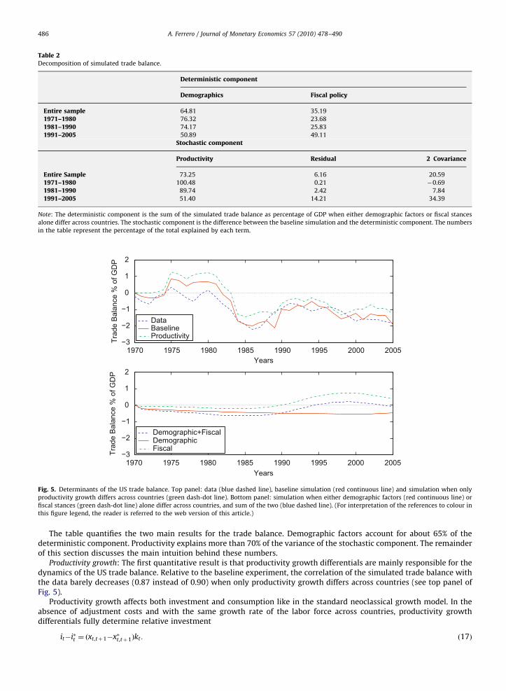
Fig. 5. Determinants of the US trade balance. Top panel: data (blue dashed line), baseline simulation (red continuous line) and simulation when only

productivity growth differs across countries (green dash-dot line). Bottom panel: simulation when either demographic factors (red continuous line) or

fiscal stances (green dash-dot line) alone differ across countries, and sum of the two (blue dashed line). (For interpretation of the references to colour in

this figure legend, the reader is referred to the web version of this article.)


The table quantifies the two main results for the trade balance. Demographic factors account for about 65% of thedeterministic component. Productivity explains more than 70% of the variance of the stochastic component. The remainderof this section discusses the main intuition behind these numbers.

Productivity growth: The first quantitative result is that productivity growth differentials are mainly responsible for thedynamics of the US trade balance. Relative to the baseline experiment, the correlation of the simulated trade balance withthe data barely decreases (0.87 instead of 0.90) when only productivity growth differs across countries (see top panel ofFig. 5).

Productivity growth affects both investment and consumption like in the standard neoclassical growth model. In theabsence of adjustment costs and with the same growth rate of the labor force across countries, productivity growthdifferentials fully determine relative investment

it�i�t ¼ ðxt,tþ1�x�t,tþ1Þkt : ð17Þ

ARTICLE IN PRESS


Higher productivity growth in the US attracts foreign resources because agents in the world economy want to hold claimsagainst capital in the country that employs it more efficiently. In addition, the wealth effect leads to temporarily higher USconsumption relative to the G6 ðct�c�t 40Þ. Expression (16) then implies that the trade balance turns negative. Asproductivity growth differentials subside, US households repay the outstanding foreign liabilities by decreasingconsumption and increasing savings. As in the data, periods of positive US productivity growth differentials (basicallythe second part of the 1980s and again since the late 1990s) corresponds to widening external imbalances.

Demographic factors: One limitation of the model with productivity growth differentials only is that it systematicallyunderpredicts the US external imbalances. The crucial implication is that demographic factors and fiscal policy differentialsaccount for a non-negligible and very persistent component of the US external imbalances with the G6. In particular, thebottom panel of Fig. 5 shows that demographic factors alone make up for almost the entire difference.

Differentials in life expectancy represent about one-half of the total effect of demographic variables on the tradebalance. Holding everything else equal, a higher surviving probability g reduces the marginal propensity to consume ofboth retirees and workers. Therefore, a longer lifetime horizon in the G6 implies a smaller marginal propensity to consumeof retirees in that region (mpcr

�) relative to the US (mpcr)

mpc�r�mpcr ¼�bsRs�1

W ðg��gÞ:

A similar channel also affects the marginal propensity to consume for workers, due to the expectation of a longerretirement period. In the aggregate, the increase in the expected lifetime horizon increases the saving rate. Workers savemore in order to finance a longer retirement period while retirees spread their consumption over a longer retirementperiod. The crucial implication for the trade balance is that, ceteris paribus, the level of savings is higher in the countrywith higher life expectancy.21 The relative excess of savings generates a trade surplus associated with the accumulation ofa positive stock of net foreign assets. The life-cycle structure of the model is the core of this mechanism.

Population growth rate differentials explain about one-quarter of the total effect of demographic variables on the tradebalance. Earlier work on the open economy relevance of demographic factors mostly focused on the role of populationgrowth rates (see the survey in Obstfeld and Rogoff, 1996), which can influence the trade balance along two conflictingmargins. On the one hand, different population growth rates across countries affect relative investments very much likeproductivity differentials

it�i�t ¼ ðnt,tþ1�n�t,tþ1Þkt , ð18Þ

where expression (18) abstracts from investment adjustment costs and productivity differentials. As for productivity, ahigher US population growth rate relative to the G6 leads to capital inflows to maintain an equal rate of return acrosscountries. On the other hand, the evolution of population growth rates influences the overall age profile of each country.Given two countries initially identical in all respects, a reduction of the population growth rate in the Foreign countryincreases the dependency ratio relative to the Home country

ctþ1

c�tþ1

¼1þn�t,tþ1

1þnt,tþ1:

Since retirees consume relatively more than workers, this channel generates an increase of aggregate consumption in thecountry with the higher dependency ratio. The simulation suggests a mild predominance of the investment channel,although the overall effect appears to be rather small.22

The interaction between differentials in life expectancy and population growth rates accounts for the remaining quarterof the overall effect of demographic factors on the trade balance. The combination of these two forces exerts a more thanproportional pressure on the dependency ratio. The number of retirees grows relative to the number of workers because (i)the average lifetime horizon is longer (aging) and (ii) fewer people are born in each period (growth). The pool of retirees islarger in the G6 than in the US. But retirees in the G6 live on average longer and, thus, need to save relatively more thantheir US counterparts.

Discussion: The quantitative predominance of productivity growth differentials in accounting for the US externalimbalances vis-a-vis the G6 is consistent with other recent studies. Engel and Rogers (2006) explain the evolution of the UScurrent account since the mid 1990s with the increase in the US share of output among advanced economies. Surveyevidence from the Consensus Forecasts supports their results. This paper identifies in productivity growth anddemographic factors the two key variables that drive the US share of world output and quantifies their relativeimportance.23

Chen et al. (2009) also stress the central role of productivity growth differentials in explaining the dynamics of the USexternal imbalances. However, their model also underpredicts the US current account by about 0.5% of GDP when only

21 A higher survival probability also increases the dependency ratio. For a given marginal propensity to consume, a larger pool of retirees drives up

aggregate consumption. However, the reduction in the retirees’ marginal propensity to consume due to the longer lifetime horizon quantitatively

dominates the effect of the change in the composition of the population.22 Higgins (1998) finds empirical support for both channels associated with population growth.23 The increase in the US share of world output in the model between 2005 and 2030 roughly coincides with the projections from Consensus

Forecasts.

ARTICLE IN PRESS

1980 1985 1990 1995 2000 20050

2

4

6

8

Years

Rea

l Int

eres

t Rat

e in

%

Data (Avg G7)BaselineProductivity

1980 1985 1990 1995 2000 20050

2

4

6

8

Years

Rea

l Int

eres

t Rat

e in

%

Data (Trend)DemographicFiscal

Fig. 6. World real interest rate. Top panel: data (blue dashed line), baseline simulation (red continuous line) and simulation when only productivity

growth differs across countries (green dash-dot line). Bottom panel: linear trend in the data (blue dashed line) and simulation when either demographic

factors (red continuous line) or fiscal stances (green dash-dot line) alone differ across countries. (For interpretation of the references to colour in this

figure legend, the reader is referred to the web version of this article.)


productivity differs across countries. In their analysis, differences in tax rates and depreciation fill the gap. Here, the gap isfilled by demographic factors, especially differentials in life expectancy.

Recently, Henriksen (2002), Feroli (2003) and Domeij and Floden (2006) also find a persistent component of US externalimbalances against other industrialized countries due to demographic factors. Differently from these studies, the simplemodel presented in the previous section combines demographic factors with other potential explanations of externalimbalances in a unified and tractable framework. More importantly, the quantitative analysis disentangles the role ofpopulation growth rates and life expectancy differentials along the demographic transition. The main finding is that lifeexpectancy is the key demographic indicator responsible for external imbalances.

Fiscal policy: The quantitative contribution of fiscal policy differentials to the US external imbalances vis-a-vis the G6 ismodest. Importantly, this result is not built into the model. To the contrary, the life-cycle structure in the model breaksRicardian equivalence and allows for potentially large effects of fiscal deficits on the net foreign asset position.24

Fiscal policy differentials affect the trade balance only through relative consumption, although the general equilibriumeffect on the world real interest rate partly mitigates the benefits of fiscal expansions on aggregate demand. Conditional ona fiscal expansion in the US relative to the G6, the model predicts that fiscal and trade deficits are ‘‘twins’’. Unconditionally,however, the data push against the twin-deficit hypothesis. The US fiscal stance has been only marginally expansionaryrelative to the G6 for the first 20 years of the sample and relatively contractionary ever since. Therefore, the model withonly fiscal differentials predicts a small trade deficit (on average, 0.13% of GDP) for the period 1970–1990 and acounterfactual trade surplus (0.5% of GDP) for the rest of the sample.25

3.3. The world real interest rate

The increase in international financial integration since the early 1980s has corresponded to a period of declining worldreal interest rates (the dashed line in Fig. 6). The ‘‘saving glut’’ hypothesis (Bernanke, 2005) interprets the evolution of realinterest rates and the US external imbalances as two aspects of the same phenomenon, both driven by a significantincrease in the world supply of savings. Recently, Caballero et al. (2008) and Mendoza et al. (2009) have formalized this

24 The effects of fiscal deficits on external imbalances are about three times as large as the estimates of Erceg et al. (2005). Under the baseline

calibration, a permanent increase in the US fiscal deficit of 1% of GDP generates a deterioration of the US trade balance at the trough of roughly 0.6% of

GDP.25 An important implication of the quantitative analysis is that the existence of fiscal surpluses and trade deficits in the US during the 1990s is not

necessarily evidence in favor of Ricardian equivalence. The US fiscal stance relative to the rest of the world, not its absolute magnitude, determines the

equilibrium effects of fiscal deficits on external imbalances.

ARTICLE IN PRESS


idea by linking the global saving glut to capital markets imperfections in emerging economies. This thesis is appealingbecause of the prominent role of emerging market economies in accounting for the growing US external imbalances afterthe Asian crises of the late 1990s. One limitation, however, is that real rates started falling in the mid 1980s acrossindustrialized countries, well before the emergence of the global saving glut.

This section discusses the relation between global imbalances and decreasing real interest rates in light of the drivingforces discussed so far. The demographic transition is the key factor to quantitatively account for the dynamics of the worldreal interest rate. In particular, the increase in life expectancy plays a crucial role in generating a reduction of the realreturn. As agents expect to live longer, the saving rate of both workers and retirees increases. Even though lowerpopulation growth rates would tend to reduce the long run world saving rate by increasing the dependency ratio, theinteraction with longer life expectancy more than compensates for this effect. The larger pool of retirees experiences onaverage a longer lifetime relative to the initial steady state. The model with only differentials in demographic factorsquantitatively accounts quite well for the decline of the world interest rate observed in the data (bottom panel of Fig. 6).

Conversely, neither measured productivity growth nor actual fiscal policies alone can explain the decrease of realreturns in international financial markets. On the one hand, productivity growth moves consumption and investment inthe same direction. These two dimensions, however, exert opposite pressures on the real interest rate. Quantitatively, themodel with only differentials in productivity growth produces a fairly flat pattern of the world real interest rate (top panelof Fig. 6). On the other hand, in the model, the effects of fiscal policy on the world real interest rate depend on the globalfiscal stance. Fiscal policy has been mildly expansionary among G7 countries during the last three decades. Therefore, themodel with only fiscal policy differentials predicts an increase in the world real interest rate which is clearly at odds withthe data (bottom panel of Fig. 6).26

The consistency of simulated and observed data for the real interest rate is an important reality check for the model.Low (and decreasing) real interest rates generally favor deficits by reducing the cost of borrowing and maintaining a lowburden of outstanding debt. This mechanism constitutes an intertemporal valuation effect which increases the persistenceof net foreign debt. Consider, for example, a gradual increase in Foreign life expectancy. In the model, such a shockgenerates a trade deficit in the Home country and puts downward pressure on the world real interest rate. Simulationresults suggest that the real interest rate absorbs approximately half of the impact adjustment in the trade balance. If theForeign country were small enough not to affect the world interest rate, the trade deficit in the Home country would betwice as big. Moreover, the decreasing interest rate along the transition implies a more persistent trade deficit and a moregradual rebalancing toward the new steady state, given the reduced burden of foreign debt.

4. Conclusions

Differentials in productivity growth and demographic factors account for the evolution of the US external imbalancesvis-a-vis the G6 during the last three decades. Productivity growth differentials explain a large fraction of the level of theUS trade balance and essentially all of its dynamics. Demographic differentials imply a non-negligible and nearlypermanent US external deficit. In addition, the demographic transition plays a critical role in generating a decline in theworld real interest rate consistent with the data. On the contrary, fiscal policy differentials are of minor importance.

One important finding is that differentials in life expectancy, rather than population growth rates, are the maindemographic indicators responsible for differences in saving patterns across countries.27 One interesting avenue for futureresearch could be developing an extended model with detailed life-cycle decisions, productivity and distortionary effects ofvarious tax policies to study to which extent the margins highlighted here and in other recent papers are in factcomplements or substitutes.

Considerations about social security systems in different regions may influence the conclusions. This aspect currentlyrepresents an important difference between the US and the G6, as well as several other countries. The sustainability ofwelfare states and the agents’ expectations of potential reforms are the crucial dimensions of this problem, particularly inlight of the current demographic trends. For example, one possible response to a longer expected lifetime horizon would bean increase, either voluntary or mandatory, of the retirement age. This topic is clearly at the forefront of the economic andpolitical debate, although most countries have yet to take explicit measures in this direction.

The main implication of the results is that capital generally flows toward relatively young and rapidly growingeconomies. Countries with these characteristics often experience large and possibly persistent external imbalances.28

Unfortunately, this conclusion is not robust outside the circle of industrialized countries. China is the obvious counter-example. The Appendix presents a three-country version of the model in which the third region is (like China) a relatively

26 The results shed some new light on the empirical (lack of) relationship between fiscal deficits and interest rates. Evans (1987) interprets the

absence of high interest rates in periods of substantial fiscal deficits (both for the US and internationally) as evidence in support of Ricardian equivalence.

However, the failure to control for demographic trends may bias the results against the hypothesis that fiscal deficits trigger a positive response of the

real interest rate.27 Chen et al. (2009) also find a negligible role for population growth differentials.28 Australia, for example, has averaged a 4.3% current account deficit relative to GDP over the last decade. During the same period, average GDP

growth exceeded 3%. Australia’s population growth rate is currently comparable to the US (around 1%) while life expectancy is only slightly higher.

Backus et al. (2009) survey external imbalances for a large cross-section of industrialized and developing countries.

ARTICLE IN PRESS


young, although fast-aging, country with strong growth performance. Perhaps not surprisingly, the quantitative resultspredict the opposite pattern of external imbalances relative to the data. This counterfactual result is one way to frame theparadox of why capital does not flow from rich to poor countries (Lucas, 1990). The introduction of financial marketimperfections, as in Caballero et al. (2008) or Mendoza et al. (2009), seems a promising approach to solve this puzzle.

Appendix A. Supplementary material

Supplementary data associated with this article can be found in the online version at doi:10.1016/j.monec.2010.04.004.

References

Attanasio, O., Kitao, S., Violante, G., 2006. Quantifying the effects of the demographic transition in developing economies. Advances in Macroeconomics 6(1) Article 2. The B.E. Journals in Macroeconomics.

Auerbach, A., Kotlikoff, L., 1987. Dynamic Fiscal Policy. Cambridge University Press, Cambridge, UK.Backus, D., Henriksen, E., Lambert, F., Telmer, C., 2009. Current account fact and fiction. NBER Working Paper No. 15525.Baxter, M., Crucini, M., 1995. Business cycles and the asset structure of foreign trade. International Economic Review 36, 821–854.Bernanke, B., 2005. The global saving glut and the U.S. current account deficit. Sandridge Lecture. Virginia Association of Economics, Richmond, VA.Blanchard, O., 1985. Debt, deficits and finite horizons. Journal of Political Economy 93, 223–247.Bohn, H., 2008. The sustainability of fiscal policy in the united states. In: Neck, R., Sturm, J.-E. (Eds.), Sustainability of Public Debt. MIT Press, Cambridge,

MA.Brooks, R., 2003. Population aging and capital flows in a parallel universe. IMF Staff Papers, vol. 50, pp. 200–221.Caballero, R., Fahri, E., Gourinchas, P.O., 2008. An equilibrium model of ‘‘global imbalances’’ and low interest rates. American Economic Review 98,

358–393.Chen, S.K., _Imrohoroglu, A., _Imrohoroglu, S., 2009. A quantitative assessment of the decline in the U.S. current account balance. Journal of Monetary

Economics 56, 1135–1147.Chinn, M., 2005. Getting serious about the twin deficits. Council on Foreign Relations, Special Report No. 10.Cooley, T., 1995. Frontiers of Business Cycle Research. Princeton University Press, Princeton, NJ.Domeij, D., Floden, M., 2006. Population ageing and international capital flows. International Economic Review 47, 1013–1032.Engel, C., Rogers, J., 2006. The U.S. current account deficit and the expected share of world output. Journal of Monetary Economics 53, 1063–1093.Epstein, L., Zin, S., 1989. Substitution, risk aversion, and the temporal behavior of consumption and asset returns: a theoretical framework. Econometrica

57, 937–969.Erceg, C., Guerrieri, L., Gust, C., 2005. Expansionary fiscal shocks and the U.S. trade deficit. International Finance 8, 363–397.Evans, P., 1987. Do budget deficits raise nominal interest rates? Evidence from six countries. Journal of Monetary Economics 20, 281–300.Farmer, R., 1990. Rince preferences. Quarterly Journal of Economics 105, 43–60.Feroli, M., 2003. Capital flows among the G-7 nations: a demographic perspective. Finance and Economics Discussion Series No. 2003-54, Board of

Governors of the Federal Reserve System.Gertler, M., 1999. Government debt and social security in a life-cycle economy. Carnegie-Rochester Conference on Public Policy 50, 61–110.Ghironi, F., 2006. Macroeconomic interdependence under incomplete markets. Journal of International Economics 70, 428–450.Gourinchas, P.O., Rey, H., 2007a. From world banker to world venture capitalist: U.S. external adjustment and the exorbitant privilege. In: Clarida, R. (Ed.),

G7 Current Account Imbalances: Sustainability and Adjustment. The University of Chicago Press, Chicago, IL.Gourinchas, P.O., Rey, H., 2007b. International financial adjustment. Journal of Political Economy 115, 665–703.Henriksen, E., 2002. A demographic explanation of U.S. and Japanese current account behavior. Mimeo, University of Oslo.Higgins, M., 1998. Demography, national savings, and international capital flows. International Economic Review 39, 343–369.Juillard, M., 1996. DYNARE: A program for the resolution and simulation of dynamic models with forward variables through the use of a relaxation

algorithm. Couverture Orange No. 9602, CEPREMAP.Kollmann, R., 1998. U.S. trade balance dynamics: the role of fiscal policy and productivity shocks and of financial market linkages. Journal of International

Money and Finance 17, 637–669.Kreps, D., Porteus, E., 1978. Temporal resolution of uncertainty and dynamic choice theory. Econometrica 46, 185–200.Lane, P., Milesi-Ferretti, G.M., 2001. Long term capital movements. In: Bernanke, B., Rogoff, K. (Eds.), NBER Macroeconomics Annual. MIT Press,

Cambridge, MA.Lucas, R., 1990. Why doesn’t capital flow from rich to poor countries? American Economic Review 80, 92–96Mendoza, E., Quadrini, V., Rios-Rull, V., 2009. Financial integration, financial development and global imbalances. Journal of Political Economy 117,

371–416.Obstfeld, M., Rogoff, K., 1996. Foundations of International Macroeconomics. The MIT Press, Cambridge, MA.Schmitt-Grohe, S., Uribe, M., 2003. Closing small open economy models. Journal of International Economics 61, 163–185.Tille, C., 2008. Financial integration and the wealth effect of exchange rate fluctuations. Journal of International Economics 75, 283–294.Weil, P., 1989. Overlapping families of infinitely-lived agents. Journal of Public Economics 38, 183–198.Yaari, M., 1965. Uncertain lifetime, life insurance and the theory of the consumer. Review of Economic Studies 32, 137–150.

a structural decomposition of the u.s. trade balance: productivity, demographics and fiscal policy

Documents