a study of sabermetrics in major league baseball: the...

A Study of Sabermetrics in Major League Baseball:

The Impact of Moneyball on Free Agent Salaries

Jason Chang & Joshua Zenilman1

Honors in Management

Advisor: Kelly Bishop

Washington University in St. Louis

April 19, 2013

Abstract

Using contract and player statistic data for Major League Baseball free agents, this paper estimates the relative effects of player attributes on player salaries over different periods of time. Moneyball is the analytical, evidence-based approach to baseball, utilizing various statistics as an indicator of player performance. Estimating a hedonic pricing model, our results show a lasting impact of Moneyball in shifting the emphasis on player valuation from observable traits to more advanced statistical analysis.

1 We would like to thank Kelly Bishop for her efforts in guiding us through the research process serving as our advisor, as well as to Seethu Seetharaman, Mark Leary, and William Bottom during the Honors in Management lecture portion of the class at Olin Business School at Washington University in St. Louis.

2

1. Introduction

Traditionally in Major League Baseball (MLB), a baseball player’s relative worth was

gauged according to recent successes such as his batting average and number of strikeouts, and

the qualitative opinions of scouts, who have seen these players in action (Lewis 2003). During

the 2002 season, a cash-strapped Oakland Athletics team, led by general manager Billy Beane

argued that current player valuation was highly inaccurate and inefficient, and that the use of

new “analytical gauges” of player performance were more telling of player contribution,

effectively unleashing hidden value from overlooked players – hence the introduction of

Moneyball to the game of baseball. As a result, sabermetrics, the specialized analysis of baseball

through objective evidence, has been accepted into the game and continues to impact different

aspects of player valuation through its continual evolution and search for other undervalued traits

in order to more accurately measure a player’s relative worth.

Ever since Moneyball was first popularized in the early 2000s, sabermetrics, the “search

for objective knowledge about baseball” (Grabiner, 1994), has continuously evolved as more

advanced statistical metrics were developed to better evaluate individual player contribution to

team wins. Previously overlooked statistics such as on-base percentage (OBP), which takes the

number of times a batter reaches base (regardless of how) over the number of plate appearances,

has now become a commonplace metric.

Given the popularization of Moneyball and the claims of unleashed hidden value

resulting from pricing mismatches in the MLB, we aim to determine if the use of sabermetrics

has impacted free-agent player salaries by comparing data from the era before Moneyball, after

Moneyball (post), and in the most recent period available (post post). Through running the

3

regression model for each respective time period, we are able to account for the time lag in the

adjustment of prices. Utilizing Rosen’s (1974) hedonic model as a revealed preference method

of estimating true value for various player statistics, we believe a player can be reduced to

various characteristics and traits that the market of MLB teams value. This also allows us to take

into consideration the possibilities of multiple interactions between various player traits.

1.1 Major League Baseball as a Market for Player Salaries

In the MLB, the season structure is broken down into spring training, the regular season,

and the postseason. Spring training serves as a series of practices and exhibition games that do

not impact the overall win/loss record, while allowing new players to audition for roster spots.

During the 162 game regular season, teams compete for one of the five playoff spots in their

respective leagues (American or National) and can do this through winning their division or

capturing a wild card spot. During the postseason, teams compete through four rounds of series

in order to win the title of World Series Champion, the goal of every team. Franchises attempt to

do this by surrounding their teams with the best facilities, coaches, and fans, but most

importantly, by assembling the optimal player roster on their team.

Price theory suggests that in an environment with perfect market information and

competition, there should be a strong correlation between player attributes and pay. The market

for players in The MLB is an example of this, as player statistics have been tracked since the

early 1900s and counting various metrics has been a major part of the game (Depken 1999),

while salary data is much more transparent than for comparable information of workers in an

office setting (Kahn 1993). In the MLB, free agents are not bound by an existing contract and

after a minimum experience requirement of six years, can market their services to other teams

4

(Dworkin 1981, Scully 1989) and this allows for a significant amount of freedom for players to

move to other teams.

1.2 Previous Economic Analyses of the Moneyball Hypothesis

Hakes and Sauer’s (2006) study contests the claim that Lewis (2003) brought forth with

his Moneyball hypothesis at the individual team level. They proposed that an efficient labor

market for players would reward on-base percentage (OBP) and slugging percentage (SLG) in

the same proportions that those statistics contribute to winning, which in turn drives team

revenue, which are in turn, funneled back towards increased wages. By setting the dependent

variable as the logarithm of annual salary on the aforementioned statistics, they were able to

confirm that OBP and SLG were undervalued at the beginning of the 2000s in the MLB as it

pertained to salary from a revenue maximization standpoint. However, this does not account for

the possibility that fans prefer watching home runs rather than walks and scoring runs through

“small ball” therefore increasing willingness to pay while disregarding win percentage.

Beneventano, Berger, and Weinberg (2012) conducted a similar study using stepwise

multiple regression models analyzing the specific impact of sabermetric statistics on offensive

run production, as well as defensive run saving measures (incorporating pitching as well as

fielding statistics) on a team level. Their final model focused only on the production of position

players and combined the sabermetric stats of weighted on-base average (wOBA) and strikeout

percent with the traditional stats of slugging percentage and on-base percentage and resulted in a

𝑅2 of 95.3% for the number of runs scored. However, they were not able to completely confirm

the original contention of the paper, as the sabermetric variables did not dominate the

explanation power in the variation of the final model’s independent variable.

5

2. Data

An important decision was choosing the appropriate seasons that would enable a

comparison of the pre-Moneyball, post-Moneyball, and post post-Moneyball periods during a

timespan in which the game of baseball did not change too drastically. Therefore we selected the

free agent signings for the 2001, 2005, and 2011 seasons. 2001 represents the last year prior to

the introduction of Moneyball in 2002 - the pre-Moneyball period; 2005 was selected to reflect

the successful implementation and adoption of the theory in the MLB - the post-Moneyball

period2; and the most recent era from 2011, highlighting the continued emphasis on quantitative

analysis - the post post-Moneyball period. All productivity variables are calculated based on

performance in the prior year, because salary is determined prior to performance as a function of

expected productivity given observed performance in previous years (Hakes & Sauer 2006).

As mentioned previously, MLB statistics are readily available through a number of

databases. We selected two primary sources of data: one regarding player statistics and another

for player contracts. Because the sources use the same unique player identification code, we are

able to merge the player contract data with the player statistics data using Stata. The data and

descriptive statistics are outlined below.

2 The Boston Red Sox won the 2004 World Series and attributed their success largely to the hiring of various sabermetricians and statistical analysts

6

2.1 Key Metrics Explained

Contract Length

Players and teams can agree to contracts of any length and value above the league

minimum of one year and the lower bounds on values that change each season without any upper

limits. Players strive to secure long-term contracts to secure their long-term financial security.

Teams, on the other hand, would rather commit to smaller sums of shorter length to maintain

future financial flexibility and avoid being locked into a large contract of an underperforming

player. Thus, the players who are successfully able to secure a long-term contract are those with

above-average-to-great recent performance with teams that have the financial backing to commit

to such an agreement.

Players who were previously above-average with recent struggles in performance or

injuries, as well as players who are merely average or below average players, with the potential

for future development typically sign shorter contracts. They understand the teams’ lack of

willingness to take a large risk and therefore, are willing to accept these contracts in order to

establish themselves as a stable producer in the long run. As a result, these players typically

accept the instability associated with a higher priced short-term contract, rather than being locked

into a long-term contract in which they would feel underpaid.

Teams are reluctant to guarantee one of the 25 major league roster spots to a severely

underperforming player and have the option to offer these players minor league contracts

attached with an invitation to the major league team’s spring training. There remains the

potential for these players to make the major league roster, in the future, without any guarantee.

7

Height

In our dataset, player height is measured in inches. The strike zone of a batter has

changed since the inception of baseball, but is defined as any pitch between the batter’s

shoulders and at least one foot from the ground that is also over the plate for all years in our

sample (MLB rulebook). As such, a shorter batter, or a batter with a lower batting stance would

have a smaller strike zone, making it more difficult for opposing pitchers. However, a short

batter would typically have shorter arms and therefore a worse ability to protect the plate and

reach to make contact on moving pitches. Taller batters are able to gain more leverage and bat

speed than shorter batters.

Stolen Bases (SB)

Stolen bases are a counting statistic measuring the number of times a baserunner safely

advances to the next base during the time the pitcher is delivering the ball to home plate. Only

2nd, 3rd, and home base can be stolen - provided that the base is open. In the event that the

defense makes no attempt to throw the base-stealer out, no stolen base is credited to the runner.

In addition to absolute speed, a successful base-stealer also needs good base-running instincts

and a good understanding of the timing of a pitcher's windup. Typically, power hitters and speed

do not go together, but the combination of those two skill sets is valued as seen in the exclusive

40 - 40 club, which consists of only four players3 who have had 40 home runs and 40 bases in a

single season as of the time of this paper.

3 The only players to achieve this feat are: Jose Canseco with the Oakland As in 1988 with 42 HR and 40 SB, Barry Bonds with the San Francisco Giants in 1996 with 42 HR and 40 SB, Alex Rodriguez with the Seattle mariners in 1998 with 42 HR and 46 SB, and Alfonso Soriano with the Washington Nationals in 2006 with 46 HR and 41 SB

8

On-Base Plus Slugging Percentage (OPS)

OPS consists of two aspects: on-base percentage (OBP) and slugging percentage (SLG).

OBP is a measure of how often a batter actually reaches base, regardless of how they got on base

(with the exception of fielder errors or obstructions) and is calculated for each player in each

season as:

𝑂𝐵𝑃 = 𝐻𝑖𝑡𝑠 + 𝑊𝑎𝑙𝑘𝑠 + 𝐻𝑖𝑡 𝐵𝑦 𝑃𝑖𝑡𝑐ℎ

𝐴𝑡 𝐵𝑎𝑡𝑠 + 𝑊𝑎𝑙𝑘𝑠 + 𝐻𝑖𝑡 𝐵𝑦 𝑃𝑖𝑡𝑐ℎ + 𝑆𝑎𝑐𝑟𝑖𝑓𝑖𝑐𝑒 𝐹𝑙𝑖𝑒𝑠

Ideally, you would want a leadoff batter to have a high OBP, such that power hitters

could bring him home. Slugging percentage, on the other hand, is a measure of batter power and

is calculated for each player in each season by weighting the number of bases gained on a hit

over total at bats as follows:

𝑆𝐿𝐺 = 𝑇𝑜𝑡𝑎𝑙 𝐵𝑎𝑠𝑒𝑠𝐴𝑡 𝐵𝑎𝑡𝑠

= (1 × 𝐵) + (2 × 2𝐵) + (3 × 3𝐵) + (4 × 4𝐵)

𝐴𝑡 𝐵𝑎𝑡𝑠

Notice that walks are excluded, as only the batter’s skill of putting a ball into play is

accounted for. As the name suggests, OPS is the sum of these two factors, serving as a

sabermetric stat measuring a batter’s ability to hit for power and to get on base:

𝑂𝑃𝑆 = 𝑂𝐵𝑃 + 𝑆𝐿𝐺

9

Ground into Double Plays (GDP)

GDP is a counting statistic that measures the times when a batter hits a ground ball that

leads to a double play, resulting in two outs. This statistic has been around for a long time -

since 1919; however, it was not valued until after Moneyball, as the impact of two outs from one

batting play is severely detrimental to the offensive efforts of a team. Note that only double

plays that are the results of a ground-out are accounted for here; rare double plays such as a

flyout-throw-out or a strikeout-throw-out are not counted, as that these do not reflect the hitters

putting a ground ball into play.

Wins Above Replacement (WAR)

The most advanced metric in use today is WAR. The theory behind WAR is to measure

a player’s contribution by comparing his performance to that of a replacement player, a below

average, readily available player either in the minor leagues or on the waiver wire. The concept

is such that the sum of every player on a team’s individual WAR should equal the teams total

wins above a team of replacement players (scaled to a floor of 51.84 wins, calculated from a

32% win rate resulting from a team of replacement players). Different sabermetricians have

unique, but very similar WAR calculations. Our data uses Sean Smith’s computation found on

the Baseball-Reference website.

The main benefit of WAR is that other advanced metrics, such as on-base percentage and

slugging percentage are most useful for the estimation of batting run creation (Winston,

Mathletics). However, batting runs is just one of many factors to solve for true net contribution

to the team for WAR.

10

WAR is composed of 6 different components that correlate to runs produced and runs

saved: (1) batting runs, (2) baserunning runs (3) grounded into double plays runs, (4) fielding

runs, (5) positional adjustment runs, and (6) replacement level runs scaled based on player’s

playing time (Smith, 2010). The first five components are relative comparisons to the league

average, encompassing one half the WAR formula; the sixth component of replacement level

measures the replacement level player’s contribution. The net calculation of WAR is simplified

to:

𝑊𝐴𝑅𝑖 = 𝑃𝑙𝑎𝑦𝑒𝑟𝑖𝑤𝑖𝑛𝑠 − 𝑟𝑒𝑝𝑙𝑎𝑐𝑒𝑚𝑒𝑛𝑡 𝑝𝑙𝑎𝑦𝑒𝑟 𝑟𝑢𝑛𝑠

(1) Batting Runs: Uses a linear weights approximation, known as the weighted average

on-base average, or wOBA, to output the true value of a hitter. The regression formula uses the

total runs scored against the weighted average of the offensive categories of walks, hit by pitch,

singles, doubles, triples, and homeruns divided by plate appearances (Tango, 2007).

(2) Baserunning Runs: Baserunning contributions come via stolen bases, as well as from

the ability to advance an extra base on a hit (i.e., turning a single into a double or scoring from

second on a single). Players’ ability to steal or advance in a particular situation on a specific

type of batted ball is compared to the league average with regards to extra bases attained on top

of additional outs compiled. Statistically, extra bases add 0.20 runs and extra outs cost 0.48 runs.

Under this framework, baserunning runs are calculated. (Smyth 1990, Tango 2007)

(3) Grounded into Double Play Runs: Grounding into a double play lowers expected runs

scored; likewise a player having the ability to beat out double plays increases expected runs

scored. Double play opportunities occur when there is a runner on 1st base and less than two

outs. Comparing how often a player hits into a double play relative to the average player can

11

reveal a gain/loss in expected runs. The difference between grounding into a double play and

avoiding the double play is roughly 0.44 runs. As such, a run saved/cost metric can show the net

impact on run creation the player had on his team (Tango, 2007).

(4) Fielding Runs: Play-by-play data for hit velocity and speed off the bat, hit type (line

drive, fly ball, or ground ball), and hit location exist for every play. The individual event files

are aggregated and based on the resulting play, fielders can be compared to the expected average

outs caused by that specific event. Thus, various statistics can be quantified such as: outfielder

arm strength based on the number of times baserunners advanced compared to the average

fielder, an infielder’s ability to turn a double play, a fielder’s ability to field a bunt, catcher stolen

base to caught stealing rating adjusted for the pitcher, and 28 positive defensive plays (i.e.,

robbing a home run) and 54 adverse defensive plays (i.e., overthrowing the cutoff man).

Comparing all advanced statistical factors determines the net run effect of a positional player’s

defensive ability. Some of the data used are not readily available to the public (Dewan, 2012).

(5)Positional Adjustment: In baseball nomenclature, teams are willing to substitute

offense for defense at the tougher defensive positions. As such, lower expected offensive

production is to be expected from the tougher positions. A ranking of positions from easiest to

most difficult is: First baseman - Left fielder - Right fielder - Third baseman - Center fielder -

Second baseman - Shortstop - Catcher. Thus, equivalent fielding runs from positions at the

left end of the spectrum are not equal. Therefore positional adjustment based on relative

difficulty of the position are required to compare and identify true defensive ability of

positional players (Tango, 2008).

(6) Replacement Level: The previously discussed metrics were used to calculate net runs

above average; however WAR ultimately compares a player to a replacement level player.

http://en.wikipedia.org/wiki/First_baseman

http://en.wikipedia.org/wiki/Left_fielder

http://en.wikipedia.org/wiki/Right_fielder

http://en.wikipedia.org/wiki/Third_baseman

http://en.wikipedia.org/wiki/Center_fielder

http://en.wikipedia.org/wiki/Second_baseman

http://en.wikipedia.org/wiki/Shortstop

http://en.wikipedia.org/wiki/Catcher

12

Logically, replacement level is below average. Setting a team of replacement level players to a

win percentage of 0.320 (51.84 wins), and given the average MLB team with a 0.500 win

percentage and a won-lost record of 81-81 implies a 29.16 wins above replacement. Hence, for

all 30 MLB teams there are 875 wins above replacement total, 59% of which are attributed to

positional players and 41% to pitchers. Under that framework, an average player, based on 650

plate appearances, would have 20 runs above replacement – this 20 is the Replacement Level

Multiplier. Replacement Level Multiplier varies slightly annually based on American League or

National League. Taking the total runs above average from the first 5 factors, and scaling player

contribution to 650 plate appearances using the Multiplier outputs the total runs above

replacement (Smith, 2010). Runs are converted to wins at roughly an 8.8 : 1 runs : wins ratio

(Smyth, 1990).

2.2 Player Contracts

The source for data on player contracts was obtained from Buzzdata.com and USA today.

Any free agent that was able to sign with any team and was signed in the given period was

included in the dataset. Minor-league free-agent signings were dropped from the dataset, as the

study pertains solely to performance in the MLB. Because of the multi-period nature of the

study, contracts were adjusted for contract length, as well as for inflation using the Bureau of

Labor Statistics’ Consumer Price Index, such that final salary amounts are reflected in 2010

dollars. The 2001 contracts were inflated by 1.27 times the original amount and the 2005

contracts were inflated by 1.15 their 2005 nominal dollars.

13

10,000,000

1,000,000

100,000

10,000

1954 1959 1964 1969 1974 1979 1984 1989 1994 1999 2004 2009

2010

U

.S.

Dol

lars

League Average

League Minimum

Table 1: Inflation Adjusted Player Salaries

Prices are expressed in constant 2010 dollars.

Table (1) provides the summary statistics for the salaries in the pre-Moneyball period of

2001, post-Moneyball period of 2005, and post post-Moneyball period of 2011 for the selected

free agents. In 2001, Alex Rodriguez signed the largest sports contract in the MLB, resulting in

the larger salary range shown above. This sample will be used in the analysis as the dependent

variable in the hedonic model.

Figure 1: MLB Salaries Over Time4

4 Data collected from www.baseballanalysts.com

Contract Season Sample Size Std. Dev. Min. Max. Mean

2001 65 5,211,581 254,000 32,100,000 6,751,4832005 76 4,452,757 488,750 18,900,000 3,768,2932011 74 4,585,868 500,000 20,300,000 3,969,363

14

Figure (1) provides a picture of the overall increasing trend in both the league minimum

and the league average salaries in the MLB since the 1950s until the 2011 season, albeit at

differing rates. There is no league maximum – only what teams are willing to pay, which may

lead to team discrepancies in overall team salary amounts, as some teams have more financial

resources than others. In our selected time span, salaries have remained relatively flat over time.

2.3 Player Statistics

We acquired a complete dataset on player statistics in the prior season to the players’ free

agency from the MLB player statistic database5. In addition to standard counting statistics, the

MLB player statistic database also has the advanced sabermetric statistics which we incorporated

into this study. Furthermore, player characteristics that remain relatively stable over time, such

as height, weight, and left-handedness or right-handedness were also retrieved from this source.

Any player who did not compete in a comparable environment to the MLB, namely players that

have played in other leagues, such as playing in the minors or internationally were dropped from

the set. Additionally, because of our focus on run production and Moneyball, only position

players were incorporated, and all pitchers were discarded.

5 Available for download from www.baseball-reference.com

15

2001 Sample (n = 65)

Variable Mean Std. Dev. Min. Max.

Contract Length (Length) 1.7538 1.6011 1 10Height 72.5385 2.1292 68 77

Stolen Bases (SB ) 4.5781 6.2534 0 30On-Base Plus Slugging (OPS ) 0.7830 0.1197 0.5550 1.1540

Ground into Double Play (GDP ) 8.3438 4.6538 1 25Wins Above Replacement (WAR ) 1.0203 1.9323 -1.40 10.1

2005 Sample (n = 76)





Table 2: 2001 Free Agent Statistics



2011 Sample (n = 74)





16

0

1

2

3

4

5

6

7

200120052011

Tables (2), (3), and (4) reflect the summary statistics for the traditional counting statistics,

Moneyball sabermetric statistics, and modern day sabermetrics. Over this decade-long period,

we can see that player performance has not drastically shifted over time, as the summary

statistics indicate. Thus, any major altercation in player pricing should be the result of differing

valuation of these player traits, rather than an actual improvement of the quality of free agent

players available on the market.

Figure 2: Free Agent Signings by Team

Figure (2) illustrates the breakdown of free agent signings during the study period by

team, with respect to each season. Some teams are more active in their free agent signings, as a

result of a larger expendable salary as well as a larger need for free agents (due to player

attrition). During our study period, the team that invented Moneyball, the Oakland Athletics,

only signed one free agent from the applicable universe.

17

3. Model & Estimation

We perform a hedonic analysis on player salaries to evaluate how player valuation metrics

changes across three periods: the period prior to the popularization of Moneyball statistical

techniques, the period after the release and subsequent popularization of these methods, and most

recent period. To quantify such changes, we run a regression of player salaries on relevant

valuation metrics for each of the three unique years.

One of the main characteristics of baseball before the release of Moneyball was team’s

reliance on scouts to evaluate players. Scouts tended to be experienced individuals who lived

and breathed baseball, whether as players themselves, coaches, or association with the sport

since childhood. Scouts tended to look beyond the basic or even advanced statistics of the

players being evaluated and analyzed more subjective traits, such as whether the player’s body

could withstand the rigors of the game, structural batting form and throwing technique, as well as

“makeup,” an analysis of the player’s family and personal ambition.

3.1 The General Model

The dependent variable is the natural logarithm of adjusted contract amount, where

adjusted contract amount (Salary) is the average salary per year of the contract. The independent

variables used to describe this amount are contract length (Length), player height in inches

(Height), stolen bases (SB), on-base percentage plus slugging percentage (OPS), number of times

grounded into double play (GDP), and wins above replacement (WAR). All independent variable

statistics were collected from the season prior to the free-agent signing, taking the total contract

18

amount divided by the number of years in the contract to arrive at an annual salary. Contract

length is included to observe whether a longer contract drove a higher salary or a smaller salary.

𝑆𝑎𝑙𝑎𝑟𝑦𝑖,𝑡 = 𝐵𝑜,𝑡 + 𝐵1,𝑡𝐿𝑒𝑛𝑔𝑡ℎ𝑖,𝑡 + 𝐵2,𝑡𝐻𝑒𝑖𝑔ℎ𝑡𝑖,𝑡 + 𝐵3,𝑡𝑆𝐵𝑖,𝑡 + 𝐵4,𝑡𝑂𝑃𝑆𝑖,𝑡 + 𝐵5,𝑡𝐺𝐷𝑃𝑖,𝑡

+ 𝐵6,𝑡𝑊𝐴𝑅𝑖,𝑡 + 𝑒𝑖,𝑡

The natural logarithm is used to control for the skewed distribution of the residuals, as

seen through “superstar” free-agent signings. We find that the relationship between salary and

corresponding statistics is best described as exponential. In doing so, the results are simplified

and the coefficients are interpreted as the percentage change in salary appropriate to each

variable.

Three seasons of free agent contract data are analyzed – 2000, 2005, and 2011. We run

the above regression equation for each of the three seasons. The statistics that are used in the

regression are from the previous season (i.e., the 2000 regression is run using the player’s

characteristics in 1999). In our regressions, we find the previous season data is to have more

explanatory power than a combination of previous years, whether a simple or a weighted

average. The purpose of the model is to show the changing tendencies of player valuation. As

such, we would expect the regression for the 2000 season to show a larger impact for the pre-

Moneyball statistics, such as height and SB variables, than for the most recent sabermetric

statistic of WAR. We would also expect the opposite effect in the regression of the 2011 season,

in that the metrics developed just prior to the 2011 season would yield the largest coefficients.

19

3.2 Independent Variables

Not including the season-specific constant, we include six independent variables on the

right-hand side of our hedonic regression. We expect that the season-specific coefficients will

vary greatly across the three regressions: 2000, 2005, and 2011.

For the pre-Moneyball period, 2000, we expect height and SB to have the strongest effect.

Height represents the essence of scout analysis as it completely ignores the accompanying player

statistics and seamlessly fits into the subjective mold of determining a player’s baseball anatomic

structure. SB represents a previously accepted simple counting metric of player speed. In its

simplicity, SB measures only the amount of times a player successfully stole any base, ignoring

the success rate, who the opposing pitcher was, and the situational factors surrounding the steal.

For the immediate post-Moneyball period, 2005, we expect OPS and the number of times

GDP to have the strongest effect. OPS has a higher causal relationship to runs produced than the

traditional counting statistics (hits, home runs) due to their efficiency nature, as it accounts for

actual runs produced. Moneyball’s thesis revolves around scoring runs while limiting outs, and

illustrates the Oakland Athletics’ use of OPS in place of the outdated evaluation techniques. To

control for the second half of the Moneyball’s theorem, we chose to look at the frequency that a

player grounded into a double play (GDP), a situation in which one play results in two outs.

Though this statistic is more of a counting metric as opposed to measuring frequency, its relative

significance would reflect a shift in how outs are valued, thus illustrating an inherent subtle yet

substantial modification in valuation methodology.

For the post post-Moneyball period evaluation of modern valuation times, 2011, we

expect the WAR statistic to have the strongest impact. As previously mentioned, WAR is an all-

20

encompassing statistics that accounts for a player’s run contribution above that of a low-level

replacement player. Relevant factors analyzed include the six factors outlined in Section 2.1. As

a new statistic, we would expect this to have a limited effect for the earlier periods.

This model has minimal colinearity concerns, as each variable analyzes a unique aspect of

the game. Though WAR consists of several similar underlying player traits, WAR is calculated

using different derivations with more explanatory power. For instance, OPS has a positive

correlation with batting runs produced. However, for the batting runs aspect of WAR, a more

advanced metric based on the league average called the weighted on-base average is used. As

such, it deviates from using OPS directly and uses a different weighting system based on the

league runs environment.

3.3 Alternative Specifications

While the intention was to measure the shift in valuation metrics, various forms of the

regression were run. Variables such as position, league, right or left-handedness, or switch

hitter, weight, and player age were included in alternative specifications. Interestingly, when

combined with the advanced metrics, none were remotely significant for any given year. Other

than stolen bases and double plays, basic counting statistics were ignored, as their impact would

be included in the OPS calculation. Furthermore, the components of OPS identify both the

frequency that a player gets on base as well as the magnitude of the player’s hits, thus

encompassing both hitting ability and power.

21

4. Results & Discussion

In this section, we discuss the results from the estimation of our log-linear hedonic salary

function, using the aforementioned model. For each pre-Moneyball, post-Moneyball, and post

post-Moneyball period, in the years (2000, 2005 and 2011, respectively), we estimate the model

described in Section 3. The regression analysis reveals that recent valuation methods have

evolved towards a more advanced statistical foundation and away from observable player traits

and counting statistics. Furthermore, these results show that the Moneyball theory has had a

tangible, lasting impact on player valuation in The MLB.

4.1 Pre-Moneyball

Table (5) shows the results from the estimation for the free agents signed in the pre-

Moneyball era (2000). In the regression of this period, the traditional observable traits of height

and SB, a proxy for player speed, are statistically significant, as we would expect. However, the

run-producing OPS variable and the out-preserving GDP variable also achieve statistical and

economic significance, suggesting that these factors were also accounted for through other

counting statistics. As expected, WAR is small and insignificant, as this metric had not yet been

created.

22

Source SS df MS F (6 , 58) 30.4Model 57.1464 6 9.5244 Prob > F 0.0000

Residual 17.8586 58 0.3133 R - Squared 0.7619Total 75.0050 64 1.1906 Adj R-Squared 0.7368

Root MSE 0.5597

Pre-Moneyball 2001 Sample (n = 65) Salaryi,t Coefficient Standard Error t - value p > | t | [95% Confidence Interval]

Contract Length (Length ) 0.1701 0.0634 2.68 0.009 0.0432 0.2970Height 0.1177 0.0358 3.29 0.002 0.0460 0.1893

Stolen Bases (SB ) 0.0400 0.0135 2.97 0.004 0.0130 0.0670On-Base Plus Slugging (OPS ) 0.0343 0.0095 3.63 0.001 0.0154 0.0532

Ground into Double Play (GDP ) 0.0775 0.0159 4.87 0.000 0.0456 0.1094Wins Above Replacement (WAR ) 0.0588 0.0757 0.78 0.440 -0.0927 0.2103

Constant 1.8815 2.7389 0.69 0.495 -3.6031 7.3662

Table 5: Pre-Moneyball regression results

Interestingly, length has a positive relationship on salary, illustrating that the longer

contracts are also the more lucrative ones. From this, it can be deduced that the players getting

signed to long-term deals are the more successful players that teams want for longer periods and

that the players sees no negative tradeoff in salary with regards to financial security. Likewise, it

shows that teams do not pay more for short-term contracts. Thus, the short-term contracts tend

to be players with less negotiating leverage. This could be because the players who sign the

shorter teams are of inferior quality or considered more risky “prospects” with fewer interested

parties in their services. Because of this, there is no presence of a bidding war and narrow

incentives for teams to offer such players financial security in the form of a larger salary or

longer length.

OPS has the largest coefficient. This is due to the fact that it is the run-producing variable

in the regression. Though the measurable player traits of height and SB are significant (p <0.05),

they do not impact performance the way OPS does, as an extra inch of height or another stolen

base is not as predictive as another run. Thus, it is logical that OPS would have a large, positive

impact. Given the percentage nature of OPS, the highest single-season figure in MLB history is

23

Pre-Moneyball 2001 Sample (n = 65, average salary = $6,751,483)Impact on Salary Coefficient Dollar Impact

Contract Length (Length ) 0.1701 1,148,389Height 0.1177 794,390

Stolen Bases (SB ) 0.0400 270,067On-Base Plus Slugging (OPS ) 0.0343 231,701

Ground into Double Play (GDP ) 0.0775 523,147Wins Above Replacement (WAR ) 0.0588 396,965

Barry Bond’s 2004 OPS of 1.4217, an increase in the coefficient of one represents an extreme

amplification of the previous number. To illustrate, an OPS of 1.0000 has only been achieved

395 times in MLB history, thus the increase itself would turn a below-average replacement

player into a probable all-star.

GDP, which results in an extra out, has a negative sign. This, however, may not be

counterintuitive. The factors that contribute to a double play go far beyond that of the batter,

including infield position, location of the batted ball, and the defense’s ability to turn the double

play. And considering batters have limited control over the ultimate location of non-home runs

batted balls (McCracken, 2001), it is understandable that teams do not look unfavorably to the

novice statistic of total ground ball double plays. Meanwhile, WAR, in addition to being

statistically insignificant also exhibits miniscule economic significance with a logarithmic

coefficient of merely 5.8%, the second smallest coefficient in this regression.

Table 6: Pre-Moneyball Dollar Impact on Average Salary

The logarithmic estimation outputs a percentage change in salary. Table (6) converts the

percentage change to reveal the monetary impact of increasing each coefficient by a one unit,

based on the sample average salary of $6.751 million during this period. According to the

regression analysis, for instance, increasing the average player’s contract length by one year

24



Root MSE 0.5560

Post-Moneyball 2005 Sample (n = 76) Salaryi,t Coefficient Standard Error t - value p > | t | [95% Confidence Interval]

Contract Length (Length ) 0.4370 0.0691 6.33 0.000 0.2992 0.5747Height 0.0228 0.0295 0.78 0.441 -0.0359 0.0816

Stolen Bases (SB ) 0.0012 0.0124 0.10 0.923 -0.0235 0.0259On-Base Plus Slugging (OPS ) 0.0146 0.0062 2.34 0.022 0.0022 0.0270

Ground into Double Play (GDP ) 0.0470 0.0141 3.34 0.001 0.0189 0.0751Wins Above Replacement (WAR ) 0.0539 0.0552 0.98 0.332 -0.0562 0.1640

Constant 10.4478 2.1055 4.96 0.000 6.2474 14.6482

would increase his annual salary by $1.148 million. An added inch to height would increase his

annual salary by $794,000. An additional SB would yield an increase of $270,000. A 1%

increase in OPS would increase salary by $232,000. Another GDP would increase a player’s

salary by $523,000. An increase of one win in WAR would result in an increase of $397,000 in

salary.

4.2 Post-Moneyball

The post-Moneyball 2005 season regression results are consistent with our hypothesis.

The height and SB variables lose their significance, WAR maintains its statistical and economic

insignificance, and OPS and GDP stay statistically significant with changes in economic

significance. However, the coefficients of OPS actually decreases, presenting a contrary view to

the theory that statistics played a larger, not a smaller, role in determining player value after the

release of Moneyball. The regression results are shown in Table (7).

Table 7: Post-Moneyball regression results

25

What we have described as a Moneyball statistic in OPS has a large and statistically

significant coefficient in both 2000 (the pre-Moneyball season) and 2005. While the general

trend between these periods was expected, the coefficient deviation is due to the inherent nature

of the regression. The pre-Moneyball variables only analyze height and speed, thereby ignoring

actual run production. Traditional power metrics, such as home runs, extra base hits, and runs

batted in, are used to observe player power. As home runs and other extra base hits factor

linearly into the OPS calculation where the slugging percentage component is the sum total bases

(weighting a home run as four times as much as a single), this variable does contain intrinsic

relevant run production explanatory power. However, given the limited sample size of roughly

seventy observations per season, the additional variables of home runs and extra base hits that

would help narrow down the true driver of run production on player valuation in the pre-

Moneyball framework could only be added at the expense of the player makeup variables.

As Moneyball represented the shift away from the input of scouts towards “hard”

statistics, we believed it was more informative to reveal that shift away from scouts between

2000 and 2005 followed by the statistical shift that was taking place continued through to 2011,

and rise of sabermetric statistics. Height has a small coefficient and 95% confidence interval [-

0.0359,0.0816], consistent with its statistical insignificance. The decrease in the OPS coefficient

illustrates the shift away from scoutable traits as the game has progressed. Contract length takes

on additional economic impact (43% versus 17%). However, contract lengths are a function of

the free agent class and ability, the better the free agent class, the higher their valuation, and the

longer length.

26

Post-Moneyball 2005 Sample (n = 76, average salary = $3,738,293)Impact on Salary Coefficient Dollar Impact

Contract Length (Length ) 0.4370 1,646,597Height 0.0228 86,053

Stolen Bases (SB ) 0.0012 4,503On-Base Plus Slugging (OPS ) 0.0146 54,936


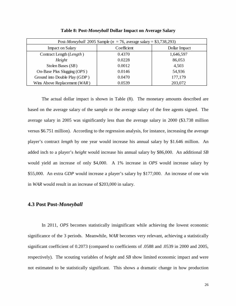
Table 8: Post-Moneyball Dollar Impact on Average Salary

The actual dollar impact is shown in Table (8). The monetary amounts described are

based on the average salary of the sample or the average salary of the free agents signed. The

average salary in 2005 was significantly less than the average salary in 2000 ($3.738 million

versus $6.751 million). According to the regression analysis, for instance, increasing the average

player’s contract length by one year would increase his annual salary by $1.646 million. An

added inch to a player’s height would increase his annual salary by $86,000. An additional SB

would yield an increase of only $4,000. A 1% increase in OPS would increase salary by

$55,000. An extra GDP would increase a player’s salary by $177,000. An increase of one win

in WAR would result in an increase of $203,000 in salary.

4.3 Post Post-Moneyball

In 2011, OPS becomes statistically insignificant while achieving the lowest economic

significance of the 3 periods. Meanwhile, WAR becomes very relevant, achieving a statistically

significant coefficient of 0.2073 (compared to coefficients of .0588 and .0539 in 2000 and 2005,

respectively). The scouting variables of height and SB show limited economic impact and were

not estimated to be statistically significant. This shows a dramatic change in how production

27



Root MSE 0.5443

Post Post-Moneyball 2011 Sample (n = 74) Salaryi,t Coefficient Standard Error t - value p > | t | [95% Confidence Interval]

Contract Length (Length ) 0.2031 0.7524 2.70 0.009 0.0530 0.3533Height 0.0549 0.0360 1.53 0.132 -0.0169 0.1267

Stolen Bases (SB ) (0.0090) 0.0108 -0.83 0.407 -0.0305 0.0125On-Base Plus Slugging (OPS ) 0.0115 0.0096 1.20 0.235 -0.0077 0.0307

Ground into Double Play (GDP ) 0.0549 0.1154 4.76 0.000 0.0319 0.0779Wins Above Replacement (WAR ) 0.2073 0.0694 2.99 0.004 0.0688 0.3457

Constant 8.8588 2.3522 3.77 0.000 4.1639 13.5538

was measured – no longer is the easy-to-calculate OPS relevant, rather the iterative statistic of

WAR data achieves significance without impairing the adjusted 𝑅2 in the modern era of baseball

as illustrated in Table (9) below.

Table 9: Post post-Moneyball regression results

Not only has WAR become significant, but also the traditional speed metric of SB has

become negative. Traditional baseball theory would suggest that the number of stolen bases

would have a positive relationship to player salary, but it appears that in this most modern era of

baseball, teams have begun to implement the valuation of efficiency ratings over counting

statistics, as seen through the statistical insignificance of SB, as well as how the 95% confidence

interval containing both positive and negative values. The GDP metric has almost become an

out-preserving metric for gauging player speed.

28

Post Post-Moneyball 2011 Sample (n = 74, average salary = $3,969,363)Impact on Salary Coefficient Dollar Impact

Contract Length (Length ) 0.2031 806,357Height 0.0549 217,869

Stolen Bases (SB ) (0.0090) (35,637)On-Base Plus Slugging (OPS ) 0.0115 45,623


Table 10: Post Post-Moneyball Dollar Impact on Average Salary

Table (10) illustrates the dollar impact seen during this period. The average salary in

2011 was $3.969 million. According to the regression analysis, increasing the average player’s

contract length by one year would increase his annual salary by $806,000. An added inch to a

player’s height would increase his annual salary by $218,000. An extra SB would yield an

decrease of $36,000. A 1% increase in OPS would increase salary by $46,000. Another GDP

would increase a player’s salary by $218,000. An increase of one win in WAR would result in an

increase of $823,000 in salary.

Of all the factors, WAR has the largest monetary impact on salary, achieving more than

twice the economic salary compared to prior years and nearly four times the economic impact.

This post post-Moneyball period highlights the importance that teams now place on advanced

sabermetric statistics, illustrating the permanent shift that Moneyball has brought to the game,

emphasizing the power of aggregating data. This also suggests the possible continual evolution

towards a “more perfect” statistic that better predicts a player’s impact on run production in the

MLB. In those future periods, we would venture that WAR would become replaced by the

newer, more advanced statistics.

29

4.3 General Trends

For all three regressions, the adjusted 𝑅2 show an explanatory power above 70%. The

lack of a dramatic change in the explanation power suggests that the six variables included in the

model consistently accounts for a significant portion of the factors that go into the valuation of

free agents. Thus, the yearly differences in player salaries are explained through a shift in the

explanatory power of the dependent variables, thereby enforcing the overarching claim of a

Moneyball shift to player valuation. Given the logarithmic nature of the regression, the

dependent variables explain salary increases in percentage, and not linear, terms. Also note that

contract length has maintained a positive and statistically significant coefficient throughout this

decade-long period, suggesting that it is only the superstars that get the security of a long-term

contract.

5. Conclusion

In this paper, we estimate the effect of quantifiable analytics on how MLB players are

valued in the open market. Moneyball is used as the framework to baseline our analysis due to

its impact in popularizing statistical thought in baseball. We employ a logarithmic regression on

three seasons of free agent contract data to illustrate how valuation techniques evolved through

the adaptation of new statistics. The three seasons used were the 2000, 2005, and 2011, each

pertaining to a period before Moneyball, immediately after Moneyball, and in the modern day.

Not including the constant, the hedonic model uses six coefficients: length, height, stolen

bases, on-base plus slugging percentage, ground into double plays, and wins above replacement.

30

The variables were chosen to reflect the metrics used to value players in each period. Through

the examination of the shift in statistical and economic significance of the variables, we find a

shift in valuation techniques away from the observable player traits and novice statistics towards

a more advanced statistical approach.

The chronological progression of WAR, the most current advanced metric, sees a positive

shift in the coefficient, describing a large increase in monetary effect, and an increase in

statistical significance. In 2011, WAR achieved a coefficient of 0.2073, with a p-value of 0.004

for a monetary impact of $823,000 per year of one increased win. In 2005, the same trait

achieved 0.0539, 0.332, and $203,000, respectively; while in 2000 WAR achieved 0.0588, 0.440,

and $397,000, respectively. The greatest economic impact occurs in 2011, consistent with our

hypothesis of a positive shift in WAR’s influence. Height, on the other hand, exhibits an opposite

trend, as it loses the statistical and economic impact it had in 2000 entirely by 2011. In 2000,

height revealed a coefficient of 0.1177 with a p-value of 0.002 for a monetary impact of

$794,000. In 2011, the coefficient drops to 0.0549, the p-value loses significance at 0.132 and

there is minimal monetary impact of merely $218,000. The 95% confidence interval for

monetary effects of height is [-67,082.23, 502,918.29]. The change in the impact of variables is

consistent from both statistical and economic significance standpoints and help reveal how

player valuations evolved and become more statistically-focused after the release of Moneyball.

31

References

Beneventano, Philip, Paul D. Berger, and Bruce D. Weinberg. "Predicting Run Production and Run Prevention in Baseball: The Impact of Sabermetrics."

Depken II, Craig A. "Free-agency and the competitiveness of major league baseball." Review of Industrial Organization 14.3 (1999): 205-217.

Dewan, John, and Ben Jedlover. The Fielding Bible. ACTA Sports, 2012.

Dworkin, James B. Owners versus players: Baseball and collective bargaining. Boston, Mass: Auburn House Publishing Company, 1981.

Grabiner, David. "The Sabermetric Manifesto." SeanLahman.com. N.p., 1994. Web. 14 Apr. 2013.

Hakes, Jahn K., and Raymond D. Sauer. "An economic evaluation of the Moneyball hypothesis." The Journal of Economic Perspectives 20.3 (2006): 173-185.

Kahn, Lawrence M. "Free agency, long-term contracts and compensation in Major League Baseball: Estimates from panel data." The Review of Economics and Statistics (1993): 157-164.

Lehn, Kenneth (1984) ‘Information Asymmetries in Baseball’s Free Agent Market’, Economic Inquiry, 22, 37–44.

Lewis, Michael. Moneyball: The art of winning an unfair game. WW Norton, 2004.

Rosen, Sherwin. "Hedonic prices and implicit markets: product differentiation in pure competition." The journal of political economy 82.1 (1974): 34-55.

Scully, Gerald W. The business of major league baseball. Chicago: University of Chicago Press, 1989.

Shanks, Bill. Scout's honor: The bravest way to build a winning team. Sterling & Ross Pub Incorporated, 2005.

Smith, Sean. "Position Player WAR Calculations and Details." Baseball-Reference.com. N.p., 2010. Web. 14 Apr. 2013.

Smyth, David. "W% Estimators." Weblog post. W% Estimators. N.p., 1990. Web. 14 Apr. 2013.

Tango, Tom M., Mitchel G. Lichtman, and Andrew E. Dolphin. The book: Playing the percentages in baseball. Potomac Books, Inc., 2007.

32

Tango, Tom. "WAR Updated on Baseball-Reference.” htttp://www.insidethebook.com/. N.p., 04 May 2012. Web. 14 Apr. 2013.Smyth, David. "W% Estimators." Weblog post. W% Estimators. N.p., 1990. Web. 14 Apr. 2013.

Winston, Wayne L. Mathletics: How Gamblers, Managers, and Sports Enthusiasts Use Mathematics in Baseball, Basketball, and Football (New in Paper). Princeton University Press, 2012.

a study of sabermetrics in major league baseball: the...

Documents