a study of the properties that influence vehicle …

A STUDY OF THE PROPERTIES THAT INFLUENCE VEHICLE ROLLOVER

PROPENSITY

Except where reference is made to work of others, the work described in this thesis is my

own or was done in collaboration with my advisory committee. This thesis does not include proprietary or classified information

Randall John Whitehead

Certificate of Approval: George T. Flowers Professor Mechanical Engineering

David M. Bevly, Chair Assistant Professor Mechanical Engineering

Nels Madsen Associate Professor Mechanical Engineering

Stephen L. McFarland Dean Graduate School


PROPENSITY


A Thesis

Submitted to

the Graduate Faculty of

Auburn University

in Partial Fulfillment of the

Requirements for the

Degree of

Masters of Science

Auburn, Alabama December 16, 2005

iii


PROPENSITY


Permission is granted to Auburn University to make copies of this thesis at its discretion, upon the request of individuals or institutions and

at their expense. The author reserves all publication rights.

Signature of the Author

Date of Graduation

iv

THESIS ABSTRACT


PROPENSITY


Master of Science, December 16, 2005 (B.M.E., Auburn University, 2003)

180 Typed Pages

Directed by David M. Bevly

In this thesis, a vehicle’s load condition is varied to investigate its impact on roll

stability and a stability threshold is derived empirically using vehicle simulation. A

vehicle model is developed and simulated using MATLAB. Experiments performed by

the National Highway Transportation and Safety Administration (NHTSA), are used to

validate the simulation. Data from these experiments is also used to validate a stability

threshold developed from the simulation.

Scaled passenger vehicles in conjunction with computer simulation have proven

to be a valuable tool in determining rollover propensity. The stability threshold is also

validated by scaled vehicle experiments. This is made possible with the lower cost and

increased safety of using a scaled vehicle versus full size passenger vehicles. A simple

electronic stability control (ESC) is then developed to keep the scaled vehicle within the

v

stability threshold. The ESC is tested using varying vehicle properties with a constant

vehicle model to see how these property changes affect the ESC’s effectiveness to

prevent rollover. The ESC is then implemented with an Intelligent Vehicle Model (IVM)

which updates the controller’s vehicle model as vehicle properties such as loading

conditions change. It is shown that an IVM greatly increases the success of ESC in

keeping the vehicle in the stability region.

vi

ACKNOWLEGEMENTS

This thesis is dedicated to my Dad and Mom, Larry and Judy Whitehead, whose

support throughout the past six years allowed this research to be conducted.

Special thanks to my faulty advisor Dave Bevly. You guided me through this

process and spurred me on to completion. Thank you for the opportunity to further my

education.

To the Auburn University GAVLAB, thank you for the technical advice, physical

data, and good laughs. To Rob Daily, lab manager, your MATLAB expertise and wealth

of knowledge on all other technical matters was invaluable to my studies. To Christof

Hamm, the ‘token’ lab EE, without his knowledge of circuits and computer software, I

would have had to learn things the “hard way.” To Will Travis, thanks for your hard

work on our research together. To Matt Heffernan, the “intellectual” discussions about

vehicle dynamics and racing aroused my curiosity and motivated me to search for

answers. To the rest of the Wilmore gang, Evan Gartley, Ren Flennigan, and Paul

Pearson, thanks for the company and long nights cramming for exams and final projects.

Thanks to the “Dungeon” inmates who fought valiantly beside me against the swarms of

fruit flies.

Thanks to Dr. George Flowers and Dr. Nels Madsen, “Mad Dog,” for being on

my thesis defense committee. Dr. Flowers thanks for revelation that Diet Coke is great,

vii

even at 8 a.m. classes. Dr. Madsen thanks for three seasons of Hitchcock League

baseball, and enlightening me to the power of the FBD ( 0≠ΣF )!

Thanks to Undergrad research assistants for staying up late with me and on

weekends to get projects complete. Thanks to Taylor Owens for all the engineering jokes

and teaming up with me in classes and triathlons. Thanks to the Auburn Formula SAE

Team for getting me started and interested in vehicle dynamics. Thanks to Bradley

Kirkland for being a good friend and roommate. Thanks to all my other friends who gave

me great memories in my years at Auburn University.

Thanks to my LORD, Jesus Christ, who taught me to trust and follow. There is

peace in knowing that no matter how bad I mess things up, He never gives up on me.

That is where I find hope. He directed all my paths. Proverbs 3:5-6.

viii

Style of Journal Used:

ASME Journal of Dynamic Systems, Measurement, and Control

Computer Software Used:

Microsoft Word 2003

ix

TABLE OF CONTENTS

LIST OF FIGURES...………………………………………………………………… xi

LIST OF TABLES.…………………………………………………………………… xv

1. INTRODUCTION

1.1 Motivation……………………………………………………………….. 1

1.2 Background and Literature Review.……...…….……………………..... 2

1.3 Purpose of Thesis and Contribution……………………...……………… 8

1.4 Outline of Thesis………………………………………………………… 9

2. VEHICLE MODEL

2.1 Introduction…...…….…………………………………………………… 11

2.2 Bicycle Model……………...……………………………………………. 12

2.3 Roll Model……………....………………………………………………. 15

2.4 Lateral Weight Transfer and Normal Wheel Loads..…..………………... 20

2.5 The Pacejka Tire Model: The ‘Magic’ Formula………………………… 22

2.6 Garage…………………………………………………………………… 28

2.7 Summary of Model Assumptions….……………………………………. 29

2.8 Summary and Conclusion……………………………………………….. 30

3. VEHICLE MODEL VALIDATION

3.1 Introduction…...…….…………………………………………………… 32

3.2 Steady State Analysis versus Transient Analysis………………………. 33

x

3.3 NHTSA Phase IV Comparison…………………………………………. 42

3.4 Auburn University GAVLAB Blazer…………………………………… 56

3.5 Lateral Weight Transfer Simulation…………………………………….. 59


4. ANALYSIS OF VEHICLE ROLLOVER STABILITY THRESHOLD

4.1 Introduction…………………….....……...…….………………………... 65

4.2 NHTSA Phase IV Loading Conditions………………………………….. 66

4.3 Stability Limit Development……………………………………………. 72

4.4 Tire Property Variation………………………………………………….. 80


5. ELECTRONIC STABILITY CONTROL DEVELOPMENT

5.1 Introduction…………………….....……...…….………………………... 86

5.2 Electronic Stability Control……...……………………………………… 87

5.3 Intelligent Vehicle Model ……...……………………………………….. 90


6. IMPLEMENTATION ON A SCALED VEHICLE

6.1 Introduction…………………….....……...….…………………….... 97

6.2 Motivation for using Scaled Vehicles……………………………… 98

6.3 Scaled Vehicle Description…………………..……………….…….. 99

6.4 Data Acquisition…………………………….…………………..…... 104

6.5 Simulation and Experiment Vehicle Dynamic Comparison………… 108

6.6 Stability Limit Development……………………………………...…. 110

6.7 Stability Limit Validation…………………………...……………...... 115

6.8 Electronic Stability Control.……..…………………….……….……. 118

xi

6.9 Intelligent Vehicle Model……………………………….………….... 120

6.10 Summary and Conclusion…………………………………………… 123

7. CONCLUSIONS

7.1 Summary……………………………………………………………….... 125

7.2 Recommendation for Future Work……………………………………… 127

REFERENCES……...……………………………………………………….……… 130

APPENDICES…...…………………………………………………………….…… 134

A Vehicle Garage…………………………………………………………. 135

B Scaled Vehicle Properties………………………………………………. 138

C Vehicle Simulation……………………………………………………... 140

xii

LIST OF FIGURES 1.1 Static Stability Factor………………………………………………………... 3

1.2 Fishhook Maneuver………………………………………………………….. 4

1.3 NHTSA’s Rollover Propensity Star Rating System…………………………. 5

2.1 SAE Vehicle Coordinate System……………………………………………. 11

2.2 Bicycle Model Free Body Diagram…………………………………………. 13

2.3 Sprung Mass Roll Free Body Diagram……………………………………… 16

2.4 Un-sprung Mass Roll Free Body Diagram…………………………………... 16

2.5 Linear vs. Non-Linear Tire Model with a Normal Force of 5 kN…………… 24

2.6 Non-Linear Tire Model with Varying Normal Forces………………………. 25

2.7 The Friction Circle…………………………………………………………... 27

2.8 2001 Chevrolet Blazer……………………………………………………….. 29

3.1 Maneuver A, S.S. Roll Model……………………………………………….. 34

3.2 Maneuver A, Transient Roll Model…………………………………………. 35

3.3 Maneuver B, S.S. Roll Model……………………………………………….. 37

3.4 Maneuver B, Transient Roll Model………………………………………….. 38

3.5 Zoom-In View of Test 2 Transient Model Wheel Load Response………….. 41

3.6 Steer Angle Input for the Fishhook 1a Maneuver…………………………… 43

3.7 J-Turn Maneuver Roll Dynamics for Experimental and Simulation Data…... 45

3.8 J-Turn Maneuver Yaw Dynamics for Experimental and Simulation Data….. 46

3.9 Auburn University GAVLAB Blazer Center of Gravity drawn in the Nominal Configuration………………………………………………………

47

3.10 Nominal Blazer Dynamics for a Fishhook 1a Maneuver……………………. 48

3.11 Auburn University GAVLAB Blazer Center of Gravity drawn in the RRR Configuration………………………………………………………………...

49

3.12 RRR Configuration Blazer Dynamics for a Fishhook 1a Maneuver 51

3.13 Auburn University GAVLAB Blazer Center of Gravity drawn in the RMB

xiii

Configuration………………………………………………………………... 52

3.14 RMB Configuration Blazer Dynamics for a Fishhook 1b Maneuver……….. 53

3.15 RMB Configuration Blazer Wheel Loads for a Fishhook 1b Maneuver……. 55

3.16 Auburn University NCAT Test Track Facility……………………………… 56

3.17 Lane Change Maneuver with the Auburn University GAVLAB Blazer……. 57

3.18 Lane Change Maneuver Yaw and Roll Angle Data for the GAVLAB Blazer 58

3.19 Roll FBD Un-Sprung Mass.............................................................................. 60

3.20 Maneuver B, Transient Roll, Front Lateral Weight Transfer………………... 62

3.21 Step Maneuver with Roll Center Height equal to Un-Sprung Mass CG Height………………………………………………………………………..

63

4.1 SIS Constant with Weight Split Variation…………………………………... 68

4.2 TWL Velocity for Weight Split Variation…………………………………... 69

4.3 Vehicle Understeer Gradient for a variation of Weight Splits………………. 70

4.4 TWL Velocity for Various CG Heights……………………………………... 71

4.5 Velocity and Yaw Dynamics at Rollover for CG Height Variation………… 74

4.6 Roll and Side Slip States at Rollover for CG Height Variation……………... 75

4.7 Roll Rate for CG Height Variation………………………………………….. 76

4.8 Lateral Tire Force at Rollover for CG Height Variation…………………….. 77

4.9 Velocity and Yaw Dynamics at Rollover for Weight Split Variation……….. 78

4.10 Roll and Side Slip Thresholds for Weight Split Variation…………………... 79

4.11 Tire Curves for Variation of Peak Lateral Tire Force (Fz =5 kN)…………… 80

4.12 Tire Curves for Variation of Tire Cornering Stiffness (Fz =5 kN)…………... 82

5.1 ESC Simulated on the Nominal Blazer Configuration………………………. 89

5.2 ESC with and without IVM for CG Height Variation………………………. 91

5.3 Effect on Dynamic Behavior due to CG Height Move without IVM……….. 92

5.4 Stability Limits for Weight Split Variation………………………………….. 95

6.1 First Generation Scale Vehicle Test bed…………………………………….. 100

6.2 Second Generation Scale Vehicle Test bed………………………………….. 102

6.3 Vehicle Control Schematic…………………………………………………... 104

6.4 First Generation IMU………………………………………………………... 105

6.5 Wireless Data Acquisition Package…………………………………………. 106

xiv

6.6 Second Generation Data Acquisition PCB Board. IMU and Microprocessor shown on top, GPS Receiver and Radio Modem shown on bottom…………

107

6.7 First Generation Scaled Vehicle Experimental versus Simulation Data…….. 109

6.8 Fishhook Steering Profile for Stability Limit Development………………… 111

6.9 Stability Limits for CG Height Variation……………………………………. 113

6.10 Stability Limits for the Weight Split Variation……………………………… 114

6.11 CG Height Variation Experiment Stability Limit…………………………… 117

6.12 Experimental Stability Limit for Variations in the CG Height……………… 118

6.13 Fishhook Maneuver with and without ESC enabled………………………… 119

6.14 Results for the Fishhook 1a with 60:40 Weight Split……………………….. 121

6.15 Results for the Fishhook 1a with 40:60 Weight Split……………………….. 122

xv

LIST OF TABLES 2.1 Linear Tire Model vs. Non-Linear Pacejka Tire Model……………………... 24

2.2 Pacejka Parameters…………………………………………………………... 26

3.1 Comparison of Models for Maneuver A…………………………………….. 36

3.2 Comparison of Models for Maneuver B…………………………………….. 39

3.3 Nominal vs. RRR Blazer Configuration…………………………………….. 49

3.4 Nominal vs. RMB Blazer Configuration…………………………………….. 52

4.1 NHTSA Phase IV Vehicle Load Configurations [Forkenbrock, 2002]……... 66

4.2 Blazer TWL Velocity in Fishhook 1b Maneuver [Forkenbrock, 2002]……... 66

4.3 Peak Lateral Tire Force Variation Results…………………………………... 81

4.4 Tire Cornering Stiffness Variation Results………………………………….. 83

5.1 ESC with and without IVM for CG Height Change………………………… 93

5.2 Blazer Stability Threshold for Two Weight Splits………………………….. 93

6.1 IMU Specifications………………………………………………………….. 108

6.2 ESC with and without IVM………………………………………………….. 123

1

CHAPTER 1

INTRODUCTION

1.1 Motivation

Over the past decade, the occurrence of rollover incidents in vehicle accidents has

received much attention due to the increase in Sport Utility Vehicle (SUV) miles driven

on the roadways and litigation claiming that engineers are to blame for designing unsafe

vehicles. The National Highway Traffic Safety Administration (NHTSA) reported in

2002 that 3% of all light passenger vehicle crashes on United States roads involve

rollover, yet rollover accidents are responsible for 1/3 of all passenger vehicle occupant

fatalities [Hilton, 2003]. The statistics reveal that SUVs rollover fatalities are more

prevalent than in cars; 59% of total fatalities in SUV accidents occurred in rollover

crashes, while rollovers accounted for only 23% of total fatalities in car accidents

[Ponticel, 2003]. There are many differences in the vehicle properties of SUVs versus

those of passenger cars. Understanding how these vehicle properties affect rollover is

important when designing a safe vehicle. 10,376 fatalities and 229,000 injuries were

caused by crashes that involved rollover in 2003 alone [FARS, 2005]. Along with lives,

there is an economic cost that can be decreased by designing vehicles that are less prone

to rollover. Motor vehicle crashes in the United States cost an estimated $231 billion in

economic costs [NHTSA, 2002]. It is easy to see that a reduction in the number of

2

vehicle rollovers can have a positive impact on the economy. By utilizing research to

understand how vehicle properties and vehicle dynamics affect rollover, both human life

and economic dollars can be saved.

1.2 Background and Literature Review

The vehicle dynamics and properties that affect the occurrence of vehicle rollover

have been studied for many years. Early vehicle rollover studies consisted of static tests

to determine a vehicle’s rollover propensity [Allen, 1990]. Statistical studies of vehicle

rollover accidents were also performed to correlate vehicle properties with rollover

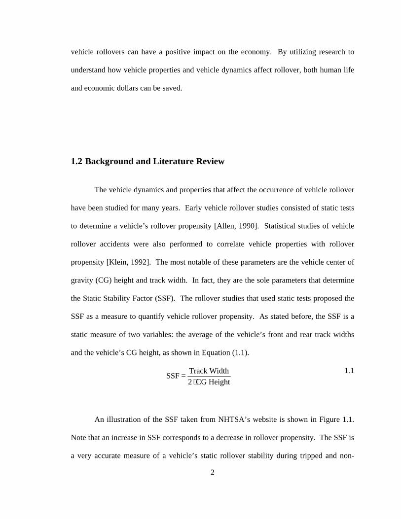
propensity [Klein, 1992]. The most notable of these parameters are the vehicle center of

gravity (CG) height and track width. In fact, they are the sole parameters that determine

the Static Stability Factor (SSF). The rollover studies that used static tests proposed the

SSF as a measure to quantify vehicle rollover propensity. As stated before, the SSF is a

static measure of two variables: the average of the vehicle’s front and rear track widths

and the vehicle’s CG height, as shown in Equation (1.1).

HeightCG 2

hTrack WidtSSF

⋅=

1.1

An illustration of the SSF taken from NHTSA’s website is shown in Figure 1.1.

Note that an increase in SSF corresponds to a decrease in rollover propensity. The SSF is

a very accurate measure of a vehicle’s static rollover stability during tripped and non-

3

tripped rollover. However, static rollover tests neglect the transient dynamics and tire

dynamics that are involved in the abrupt changes in velocity and steer angle that come

before crashes [Chrstos, 1992]. It is noted that suspension characteristics during

dynamics tests are important when determining a vehicle’s rollover stability and since

tires are non-linear, the tires’ lateral forces saturate during extreme maneuvers [Hac,

2002].

Figure 1.1. Static Stability Factor [NHTSA, 2005]

In the 1990’s, the National Highway Traffic Safety Administration’s (NHTSA)

vehicle safety star rating system used only the SSF to determine a vehicle’s rollover

propensity. However, due to the high fatality rate of rollover crashes, Congress passed

the “Transportation Recall, Enhancement, Accountability and Documentation Act,”

(TREAD), in November of 2000. TREAD charged NHTSA to conduct dynamic rollover

resistance rating tests, which NHTSA in turn made part of its New Car Assessment

Program (NCAP). For the purposes of a dynamic rollover resistance rating test, NHTSA

selected the Fishhook steering maneuver as a primary candidate to use in conducting

4

rollover experiments. An illustration of the Fishhook maneuver, taken from NHTSA’s

website is shown in Figure 1.2.

Figure 1.2. Fishhook Maneuver [NHTSA, 2005]

For vehicle dynamic testing, the rollover propensity of a vehicle is determined

from the highest speed for which the vehicle can complete the selected maneuver without

achieving two-wheel lift. Since the vehicle testing is conducted on-road, the results are

more repeatable and give more control over the test environment than off-road tripped

tests [Forkenbrock, 2003]. The evaluation procedure is only meant to test vehicles for

on-road, un-tripped, rollover propensity. Although this only accounts for a small

percentage of rollover crashes, the results are still a valuable measure of overall rollover

stability for relative comparison of vehicles [Viano, 2003]. In 2004, NHTSA added the

dynamic test to its star rating system for rollover propensity. Figure 1.3 shows NHTSA’s

5

chart for determining a vehicle’s rollover propensity star rating. It uses both the SSF and

dynamic test results in order to determine rollover propensity. However, because the

majority of rollover events are tripped and the CG height and track width are the vehicle

properties that have the greatest effect on tripped rollover propensity, the new rating

system placed more weight on the SSF [Cooperrider, 1990].

Figure 1.3. NHTSA’s Rollover Propensity Star Rating System [NHTSA, 2005]

Along with developing a rollover propensity rating system, the Department of

Transportation (DOT) has taken other action to make vehicles safer. In 2004, all new

vehicles were mandated by the DOT to have a tire pressure monitor in each tire and a tire

pressure warning light visible to the driver. The light acts as an indicator to the driver

that the tire with low pressure is a hazard and needs to be repaired. This mandate was a

6

result of the occurrence of multiple incidents in which tires with low pressure blew-out

on highways and resulted in rollover fatalities.

Electronic Stability Control (ESC) is the current buzz technology in automotive

industry, and rightly so. NHTSA has published reports stating that ESC reduces single

vehicle crashes by 67% and fatal crashes by 64%. The 10,376 rollover related fatalities

in 2003 and the 8,476 single vehicle rollover fatalities reveal the potential that ESC has to

save lives [FARS, 2005]. The ESC is designed and implemented in order to help the

driver maintain vehicle stability, while tracking the` driver’s desired path. The first

generation of ESC uses a lateral accelerometer and a yaw rate gyroscope (gryo) to

monitor the yaw dynamics and use the vehicle’s antilock braking system to brake the

wheels independently to minimize understeer and oversteer [van Zanten, 2000]. ESC’s

effectiveness is so impressive that Daimler-Chrysler, Ford, and General Motors have

announced that ESC, once only an option on SUVs, will be a standard feature in all of

their 2007 SUV models [Voelcker, 2005].

Since the first generation of ESC systems were so successful, continuous efforts

to improve ESC are ongoing [Hac, 2004]. The accurate detection of vehicle rollover and

vehicle state estimation are current topics being studied [Johansson, 2004]. The ability to

precisely estimate vehicle states such as side slip angle and slip angle rate greatly

increases the ESC’s ability to detect instability and prevent rollover [Bevly, 2001; Ryu,

2004; Nishio, 2001]. Many researchers are putting emphasis on the design and

implementation of new actuators, such as active suspension and steer-by-wire, to improve

ESC performance [Wilde, 2005; Huang, 2004; Vilaplana, 2004]. And even more ESC

research is being conducted on improving control algorithms by optimizing the use of the

7

actuators and sensors in conjunction with vehicle state estimation [Carlson, 2003;

Plumlee, 2004; Schubert, 2004].

Vehicle modeling of rollover and vehicle dynamics that influence rollover has

been studied much in recent years in order to better understand and prevent rollover

[Nalecz, 1993]. LaGrange’s method, an energy method, works well with impact

modeling such as tripping [Ginsberg, 1998]. Tripped rollover scenarios are most

commonly modeled using LaGrange’s method, although researchers have used both

Lagrange’s and Newton’s method to develop models for untripped rollover events

[Garrott, 1992; Day, 2000;]. Newton’s method works in modeling non-impact dynamics

like a vehicle’s yaw dynamics as seen in the bicycle model [Baumann, 2004].

Scaled vehicles are being used as valuable research tools to investigate vehicle

yaw dynamics and test ESC algorithms [Travis, 2004; Brennan, 2003]. The rollover

testing of full-size vehicles is an expensive and dangerous endeavor, unlike scaled

vehicles where the vehicles are cheaper and experiments are safer [Yih, 2000]. If results

from scaled vehicles tested in a controlled environment can be related to the dynamic

behavior of full-size vehicles, then the use of scaled vehicles can be an effective means of

investigating rollover [Brennan, 2001]. Brennan and Alleyne developed the Illinois

Roadway Simulator for design and evaluation of yaw dynamics controllers [Brennan,

1998]. The Illinois Roadway Simulator research and scaled vehicle experiments at

Auburn University have shown that scaled vehicle test beds are successful in capturing

the vehicle’s dynamics and can be used to develop ESC technologies for full size

passenger vehicles [Whitehead, 2004; Brennan, 2004].

8

1.3 Purpose of Thesis and Contribution

It is well known that center of gravity height and track width, the two parameters

that make up the SSF, are the major vehicle parameters that contribute to rollover

propensity. In this thesis, the effects of other vehicle properties, such as longitudinal

weight distribution, are evaluated to determine its influence on rollover propensity, while

holding the SSF constant. The purpose of this work is to analyze vehicle rollover

utilizing vehicle simulation and vehicle experimental data. A non-linear vehicle model is

created in order to study how vehicle properties affect rollover propensity. A detailed

development and description of a vehicle simulation, including validation testing, and a

discussion of the results for several parametric variation studies are provided.

An instrumented scaled vehicle is used for the first time to study vehicle rollover

and relate it to full scale passenger vehicles. The scaled vehicle is used to acquire vehicle

dynamics data leading to rollover and to evaluate a stability threshold created by

simulation. The vehicle simulation correlates the scaled vehicle with a full scale

passenger vehicle in order to validate the use of scaled vehicles for studying rollover.

The vehicle simulation is also used to develop a stability threshold which is a function of

the vehicle’s loading condition.

This work also develops a method to increase the effectiveness of ESC. Although

ESC’s ability to prevent single vehicle rollover is already high, there is room for even

more improvement by using an Intelligent Vehicle Model (IVM). The IVM utilizes

information about the vehicle to update the ESC’s vehicle model and controller limits

with a new stability threshold as the vehicle’s loading condition changes. This thesis

uses simulation in conjunction with an ESC on a scaled vehicle test bed to determine the

9

effectiveness of the ESC as vehicle properties change. The simulation is used to

determine the vehicle’s stability threshold at different vehicle properties. The ESC with

the IVM utilizes the property changes to the vehicle model and the controller gains are

adjusted to keep the vehicle within the stability threshold. This is different from a regular

ESC where the vehicle model does not change, and one stability threshold is used at all

times. Vehicle loading conditions are the most common way vehicle properties are

varied. This thesis focuses on the influence of two of those properties, CG height and

weight split, and compares the effectiveness of ESC with and without the use of an IVM.

1.4 Outline of Thesis

The purpose of this study is to evaluate and determine the parameters that

influence or change vehicle rollover propensity using both experimental data and

simulation. The first step was to derive a vehicle model for the simulation. The vehicle

model was developed using Newton’s laws of motion. The free body diagrams,

equations, and assumptions are shown in Chapter 2 [Newton, 1687]. The computer

simulation uses a transient roll and yaw dynamic model to capture the dynamics of the

vehicle. The vehicle model is verified via comparison with experimental data from a

passenger vehicle in Chapter 3. The vehicle properties’ values used are given in

Appendix A.

10

The loading conditions that effect vehicle rollover are evaluated in Chapter 4.

The vehicle model developed in Chapters 2 and 3 is used to create a stability threshold

for variations of these loading conditions. In Chapter 5, an ESC that uses throttle and

steering control to maintain vehicle stability is developed. The ESC is evaluated in

simulation and a method to improve its effectiveness is tested. The IVM, which updates

the ESC’s vehicle model and stability threshold for variations in vehicle load

configuration, is developed in this chapter and is shown to increase the ESC’s

effectiveness.

Finally, to aid in studying rollover propensity, this research uses an instrumented

scaled vehicle test bed to validate the vehicle model, the stability threshold, the ESC and

the IVM that were developed in Chapters 2-5. The scaled vehicle is instrumented with a

six degree of freedom (DOF) inertial measurement unit (IMU) and a global positioning

system (GPS). The scaled test bed is also equipped with a CG relocator which allows the

vehicle’s loading condition to be varied in the longitudinal and vertical axes. The

detailed analysis of rollover using a 1/10th scaled vehicle is given in Chapter 6. Appendix

B contains the values of the scaled vehicle properties and a description of how the roll

mass moment of inertia was quantified.

11

CHAPTER 2

VEHICLE MODEL

2.1 Introduction

In this chapter, the model of a typical four-wheel passenger vehicle is developed.

The developed vehicle model has three degrees of freedom (DOF) and was developed by

deriving the equations of motion (EOM) using the free body diagrams (FBD) of the

sprung and un-sprung masses. The vehicle coordinate system can be seen in Figure 2.1.

The primary dynamics of concern in this thesis are the yaw and roll motions.

Figure 2.1. SAE Vehicle Coordinate System [Milliken, 1995]

12

The pitch dynamics (which cause longitudinal weight transfer) are neglected since

longitudinal accelerations were kept small in the experiments considered in this thesis.

The model, which is implemented using the MATLAB programming language, was

developed to be extremely flexible. Individual vehicle properties such as center of

gravity location and suspension setup are easily changed. Additionally, the simulation

can utilize either use the transient yaw equations with either the steady state roll dynamic

equations or the transient roll dynamic equations. The difference in these two models is

apparent when analyzing the vehicle dynamics of transient maneuvers. However, in

steady state maneuvers, the difference is small, as is shown in Chapter 3.

2.2 Bicycle Model

The transient yaw equations are derived from the “bicycle model” free body

diagram shown in Figure 2.2. The 2-wheel bicycle model is the most commonly known

version; however, for the purposes of this research, a 4-wheel bicycle model is used so

that lateral weight transfer can be included in the yaw dynamics. The 4-wheel bicycle

model, assumes that the slip angles are symmetric about the x-axis of the vehicle, which

is valid at high speeds and zero Ackerman Effect [Gillespie, 1992].

13

Figure 2.2. Bicycle Model, Yaw FBD

The tire forces and slip angles in Figure 2.2 are drawn using a positive sign

convention. In actuality, the tire slip angles as shown would produce a negative lateral

tire force as shown in Figure 2.2. Summation of moments about the center of gravity

yields the yaw acceleration found in Equations (2.1 and 2.2).

[ ]mNrIM zz ⋅⋅⋅=Σ & 2.1

( )[ ] [ ]2/cos1

sradaFbFI

r yfyrz

⋅⋅⋅+⋅−⋅= δ&

2.2

where:

a = Length between the CG and front tire patch V = Vehicle velocity vector

b = Length between the CG and rear tire patch Vf = Front tire velocity vector

δ = Steer angle Vr = Rear tire velocity vector

Fy = Tire lateral forces Vx = Vehicle velocity in the x-axis

r = Yaw rate Vy = Vehicle velocity in the y-axis

14

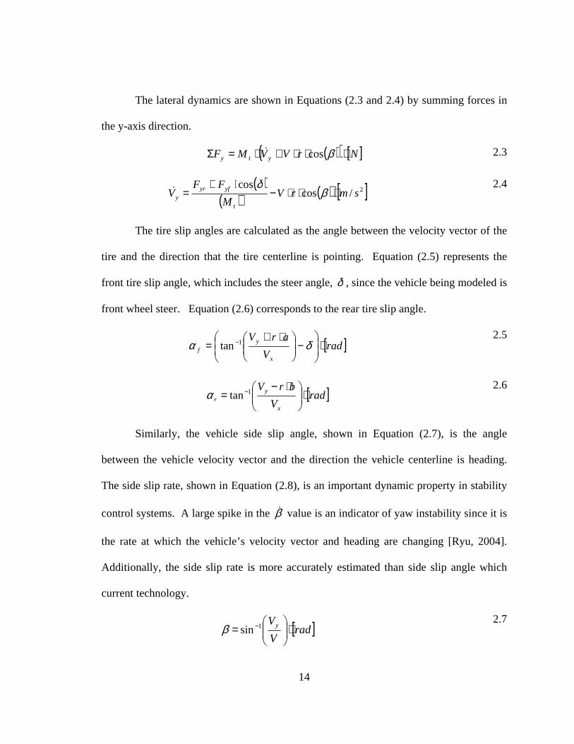
The lateral dynamics are shown in Equations (2.3 and 2.4) by summing forces in

the y-axis direction.

( )( ) [ ]NrVVMF yty ⋅⋅⋅+⋅=Σ βcos& 2.3

( )( ) ( ) [ ]2/cos

cossmrV

M

FFV

t

yfyry ⋅⋅⋅−

⋅+= β

δ&

2.4

The tire slip angles are calculated as the angle between the velocity vector of the

tire and the direction that the tire centerline is pointing. Equation (2.5) represents the

front tire slip angle, which includes the steer angle, δ , since the vehicle being modeled is

front wheel steer. Equation (2.6) corresponds to the rear tire slip angle.

[ ]radV

arV

x

yf ⋅

−

⋅+= − δα 1tan

2.5

[ ]radV

brV

x

yr ⋅

⋅−= −1tanα

2.6

Similarly, the vehicle side slip angle, shown in Equation (2.7), is the angle

between the vehicle velocity vector and the direction the vehicle centerline is heading.

The side slip rate, shown in Equation (2.8), is an important dynamic property in stability

control systems. A large spike in the β& value is an indicator of yaw instability since it is

the rate at which the vehicle’s velocity vector and heading are changing [Ryu, 2004].

Additionally, the side slip rate is more accurately estimated than side slip angle which

current technology.

[ ]radV

Vy ⋅

= −1sinβ

2.7

15

( ) ( ) [ ]sraddt

nn/

1 ⋅

−+= βββ& 2.8

The lateral acceleration, shown in Equation (2.9), is comprised of yV& and the

component of centripetal acceleration, shown in Equation (2.10), that is perpendicular to

the vehicle velocity vector.

( )( ) [ ]2/cos smaVa cenyy ⋅⋅+= β& 2.9

[ ]2/ smVracen ⋅⋅= 2.10

The vehicle’s longitudinal and lateral velocities are defined by Equations (2.11 and 2.12).

( ) [ ]smVVx /cos ⋅= β 2.11

( ) [ ]smVVy /sin ⋅= β

2.12

2.3 Roll Model

The roll equations are derived by separating the sprung and un-sprung masses in

the y-z plane, as shown in Figures 2.3 and 2.4, and applying Newton’s second law (as

formulated for rigid bodies). ‘Inside’ and ‘Outside’ represent the sides of the car that

correspond to the inside and outside of a turn. In the figures shown below, the front of

the vehicle is pointing into the page resulting in a positive roll angle towards the outside

of the vehicle.

16

Figure 2.3. Roll FBD Sprung Mass

Figure 2.4. Roll FBD Un-Sprung Mass

Fyi

Fzi

Fzo

Ry

Rz

rc

CGm

Fbi + Fki

Fbo + Fko

mg

Inside

Outside

Fyo

S/2

trk

Marb

Φ

CGM

Mg Fbi + Fki

Fbo + Fko

Inside Outside

Ry

Rz

rc

d1

Marb

17

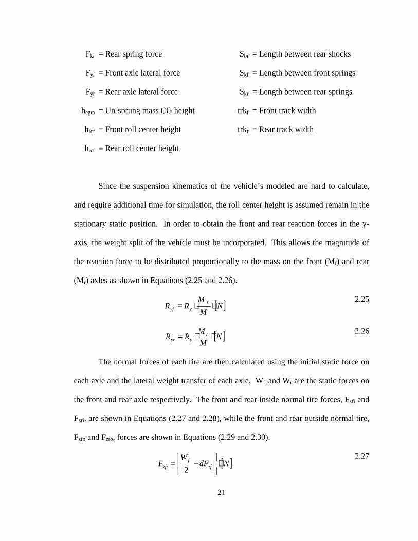
The forces, moment, and lengths on Figures 2.3 and 2.4 are defined as:

CGM = Sprung mass center of gravity Marb = Anti-roll bar moment

CGm = Un-sprung mass center of gravity Φ = Roll angle

d1 = Length between the rc and CGM rc = Roll center

Fb = Damper force

(o – outside, i – inside)

Ry = Reaction force in the y-axis

Fk = Spring force

(o – outside, i – inside)

Rz = Reaction force in the z-axis

Fy = Tire lateral force S = Length between the springs and

dampers

Fz = Tire normal force trk = Track width

The steady state roll model can be derived, by setting the acceleration and

velocity dynamic states to zero. With this simplification, roll angle is analyzed as a linear

function of lateral acceleration. This assumes that the total roll stiffness is linear and d1 is

constant due to the small angle linearization. Equation (2.13) is the linearized roll angle

equation.

[ ]radg

a

dWk

dW y

tt

tss ⋅

⋅−⋅=Φ

Φ 1

1 2.13

where:

ay = Lateral acceleration kΦt = Total roll stiffness

g = Gravitational constant Wt = Total sprung weight

18

The transient roll model is more complex than the steady state version since it is

non-linear and includes the acceleration and velocity states. The transient roll model is

very useful in that it incorporates the transient dynamics into the lateral weight transfer

equations which monitor the normal forces on the wheels. Also, roll rate is a vehicle

state of much importance in anti-rollover stability control systems. With the roll EOM,

the roll rate magnitude can be compared with rollover incidents to develop limits for a

new stability control systems. The roll equation of motion is found in Equations (2.14

and 2.15) by summing the moments about the x-axis.

[ ]mNIM xx ⋅⋅Φ⋅=Σ && 2.14

( ) ( )[ ] [ ]211 /)cos()sin(

1sraddRdRRDMRSM

I yzx

⋅Φ⋅⋅+Φ⋅⋅+−−⋅

=Φ&&

2.15

In the above equation, Φ&& is the roll acceleration, RSM is the torque from the roll

stiffness, and RDM is the torque from the roll damping. The roll stiffness (RS) and roll

stiffness moment (RSM) values are calculated in Equations (2.16 and 2.17).

( ) ( )[ ] [ ]radmNkkSkSkRS arbrarbfkrsrkfsf /5.05.0 22 ⋅⋅++⋅⋅+⋅⋅=

2.16

( ) ( )[ ][ ] [ ]mNkkSkSkRSM arbrarbfkrsrkfsf ⋅⋅Φ⋅++⋅⋅+⋅⋅= 22 5.05.0

2.17

Additionally, the roll damping (RD) and roll damping moment (RDM) are

represented by Equations (2.18 and 2.19) respectively.

( ) ( )[ ] ( )[ ]sradmNSbSbRD brrbff //5.05.0 22 ⋅⋅⋅⋅+⋅⋅=

2.18

( ) ( )[ ][ ] [ ]mNSbSbRDM brrbff ⋅⋅Φ⋅⋅⋅+⋅⋅= &22 5.05.0

2.19

19

where:

bf = Front shock damping ksr = Rear spring stiffness

br = Rear shock damping Sbf = Length between front shocks

karbf = Front anti-roll bar stiffness Sbr = Length between rear shocks

karbr = Rear anti-roll bar stiffness Skf = Length between front springs

ksf = Front spring stiffness Skr = Length between rear springs

The x and y axes reaction Forces at the roll center are given by Equations (2.20

and 2.21). Where M is the sprung mass.

[ ]NaMR yy ⋅⋅= 2.20

[ ]NgMRz ⋅⋅= 2.21

It is important to note that the roll centers are assumed to be stationary to simplify

the model. Also note that the spring and damper forces are assumed to be symmetric

about the x-axis. This is due to the complexity of calculating the suspension kinematics

during simulation. By not calculating the suspension kinematics during maneuvers, the

simulation runtime is decreased. By comparison with experimental data, it is revealed in

following chapters that this simplification is valid.

In order to simplify the lateral weight transfer calculation, the un-sprung mass roll

dynamics are neglected. The un-sprung mass transient dynamics are neglected because

rollover detection is possible by using the less complex steady state equations. The

transient dynamics for the un-sprung mass are needed to determine the height of wheel

lift. However, for this study, only the instant that the wheel is lifted is required to signal

a rollover event.

20

2.4 Lateral Weight Transfer and Normal Wheel Loads

The lateral weight transfer is derived from the un-sprung mass FBD. The lateral

weight transfer is measured as the difference between the inside and outside tire normal

forces as shown in Equation (2.22).

[ ] [ ]NFFdF zizoz ⋅−= 2.22

To accurately determine the normal force on each wheel, the FBD of the un-

sprung mass must be configured using both front and rear components. However, only

the steady state roll dynamics of the un-sprung mass are modeled since the simulation is

only concerned with rollover occurrences. Once wheel lift is detected, (which is when

the transient roll dynamics of the un-sprung mass would be critical), the vehicle

simulation is terminated and declared a rollover event. Therefore, the lateral weight

transfer of the front and rear axles are found using Equations (2.23 and 2.24),

respectively.

( )[ ] [ ]NhFhhRFSFSM

trkdF cgmyfcgmrcfyfbfbfkfkfarbf

fzf ⋅⋅+−⋅+⋅+⋅+⋅= 2

2.23

( )[ ] [ ]NhFhhRFSFSM

trkdF cgmyrcgmrcryrbrbrkrkrarbr

rzr ⋅⋅+−⋅+⋅+⋅+⋅= 2

2.24

where:

Fbf = Front damper force Ryf = Reaction force on the front

Fbr = Rear damper force Ryr = Reaction force on the rear

Fkf = Front spring force Sbf = Length between front shocks

21

Fkr = Rear spring force Sbr = Length between rear shocks

Fyf = Front axle lateral force Skf = Length between front springs

Fyr = Rear axle lateral force Skr = Length between rear springs

hcgm = Un-sprung mass CG height trkf = Front track width

hrcf = Front roll center height trkr = Rear track width

hrcr = Rear roll center height

Since the suspension kinematics of the vehicle’s modeled are hard to calculate,

and require additional time for simulation, the roll center height is assumed remain in the

stationary static position. In order to obtain the front and rear reaction forces in the y-

axis, the weight split of the vehicle must be incorporated. This allows the magnitude of

the reaction force to be distributed proportionally to the mass on the front (Mf) and rear

(Mr) axles as shown in Equations (2.25 and 2.26).

[ ]NM

MRR f

yyf ⋅⋅=

2.25

[ ]NM

MRR r

yyr ⋅⋅=

2.26

The normal forces of each tire are then calculated using the initial static force on

each axle and the lateral weight transfer of each axle. Wf and Wr are the static forces on

the front and rear axle respectively. The front and rear inside normal tire forces, Fzfi and

Fzri, are shown in Equations (2.27 and 2.28), while the front and rear outside normal tire,

Fzfo and Fzro, forces are shown in Equations (2.29 and 2.30).

[ ]NdFW

F zff

zfi ⋅

−=

2

2.27

22

[ ]NdFW

F zrr

zri ⋅

−=2

2.28

[ ]NdFW

F zff

zfo ⋅

+=

2

2.29

[ ]NdFW

F zrr

zro ⋅

+=2

2.30

2.5 The Pacejka Tire Model: The ‘Magic Formula’

The normal forces of the tires are not only used to determine vehicle rollover;

they must be used in order to determine the lateral force of each tire. Through the years,

many tire studies have been conducted resulting in various tire models. As early as 1925,

a researcher named Broulhiet discovered the concept of side slip and its role in producing

lateral forces in a pneumatic tire [Broulhiet, 1925]. Fromm also contributed to the early

studies of tire side slip and yaw [Fromm, 1954]. In the ‘50s and ‘60s, the “friction circle”

was developed and experiments were conducted in order to understand its effects on

handling [Radt, 1960; Ellis, 1963; Radt, 1963; Morrison, 1967]. In 1970, Dugoff, in

conjunction with the Highway Safety Research Institute at the University of Michigan,

published a study in which tire experiments were conducted resulting in an analytical tire

model [Dugoff, 1969; Dugoff, 1970]. A lead engineer in tire research throughout the

‘60s, Hans Pacejka, published the ‘Magic Formula’ in 1987 for use in determining the

lateral forces for a pneumatic passenger vehicle tire in vehicle simulations [Pacejka,

23

1987]. In the 1987 study, Pacejka and his colleagues recorded tire data on vehicles and

developed an equation that models the empirical data of the tire’s dynamics quite well.

In 1989, Pacejka published an even more refined and detailed “Magic Formula” [Pacejka,

1989]. This tire model is a highly non-linear model where lateral force is a function of

the tire slip angle and tire normal force. Additionally, the tire model contains parameters

such as peak tire lateral force, cornering stiffness, and tire model curvature which can be

modified to capture the effects for different tires. Not only does the “Magic Formula”

model the tire’s lateral dynamics, it contains the tire’s longitudinal dynamics as well.

The vehicle model in this research uses the Pacejka model because of its accuracy and

ease of use.

Figure 2.5 shows the difference between the linear and non-linear “Magic

Formula” tire model. The linear model has a constant tire cornering stiffness, Cα, with no

saturation, while the Pacejka tire model has a non-constant Cα as the tire curve transitions

into the non-linear region. In the non-linear Pacejka tire model, once the peak force is

reached, the lateral tire force decreases with increasing tire slip angle. This is called tire

saturation.

24

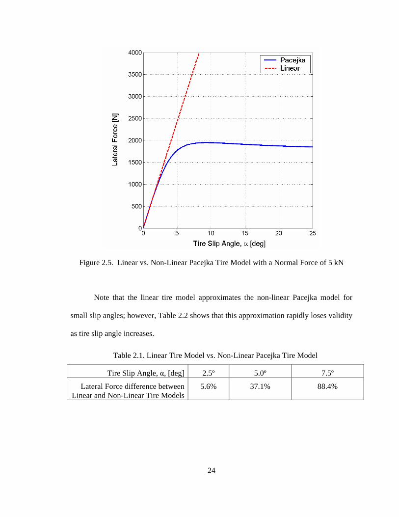
Figure 2.5. Linear vs. Non-Linear Pacejka Tire Model with a Normal Force of 5 kN

Note that the linear tire model approximates the non-linear Pacejka model for

small slip angles; however, Table 2.2 shows that this approximation rapidly loses validity

as tire slip angle increases.

Table 2.1. Linear Tire Model vs. Non-Linear Pacejka Tire Model

Tire Slip Angle, α, [deg] 2.5º 5.0º 7.5º

Lateral Force difference between Linear and Non-Linear Tire Models

5.6% 37.1% 88.4%

25

The peak tire lateral force is a function of tire slip angle and normal load. Note

that increasing normal load reaches a point where it no longer produces significant gains

in lateral force. This relationship is seen in Figure 2.6, which shows that both the Cα and

peak force change with changing normal load.

Figure 2.6. Non-Linear Tire Model with Varying Normal Forces

The inputs of the Pacejka tire model are tire slip angle and tire normal force, and

the output is tire lateral force. The non-linear Pacejka lateral tire force is calculated using

the Equation (2.31).

( )( )φ⋅⋅⋅= BaCDFy tansin 2.31

Equations (2.32 to 2.36) show the constants that are found in Equation (2.31).

Equation (2.32) is known as the shape factor, which is independent of the tire normal

force.

26

3.1=C 2.32

Equation 2.29 represents the peak factor which determines the peak lateral force

of the tire curve.

zz FaFaD ⋅+⋅= 22

1 2.33

Equation 2.30 controls the curvature of the tire curve, thus it is called the curvature

factor.

872

6 aFaFaE zz +⋅+⋅= 2.34

The cornering stiffness, αC , factor is found in equation 2.31. Where the BCD

variable is effectively αC .

( )( )zFaaaaBCD ⋅⋅⋅= 543 tansin 2.35

Equation 2.32 is developed to be used later in equation 2.33.

( ) ( )ααφ ⋅⋅

+⋅−= BaB

EE tan1

2.36

The Pacejka parameters used in the model are those found in Pacejka, 1987, and

can be seen in Table 2.2. Note that these parameters assume that the dimensional unit for

the tire slip angle is degrees and for the tire normal force is kilo-Newton. The output of

the Pacejka model, lateral tire force, has units of Newtons.

Table 2.2 Pacejka Parameters

a0 = 0 a5 = 0.208 a1 = -22.1 a6 = 0 a2 = 1011 a7 = -0.354 a3 = 1078 a8 = 0.707 a4 = 1.82

27

Steps were taken to simplify the non-linear tire model in this vehicle model. In

Figure 2.8, the radius of the friction circle represents the maximum magnitude of force

that the tire can produce at any one time. If the vehicle is braking or accelerating

(longitudinal axis), the maximum lateral force decreases from the non-braking, non-

accelerating scenario. The longitudinal effects of braking and acceleration were

neglected since the majority of the experiments were conducted at a constant longitudinal

velocity.

Figure 2.7. The Friction Circle

Only the lateral forces of the tire model are considered in this model, and some of

those are left out as well. For instance, all forces that come from camber thrust and all

moments from the self aligning torque are neglected. However, following chapters will

Longitudinal Force

Lateral Force

Braking

Forward Acceleration

Maximum Total Force Produced by the Tire

28

show how the model accurately captures a passenger vehicle’s dynamics without these

tire parameters.

2.6 Garage

The simulation uses a MATLAB m-file entitled ‘Garage.’ This appropriately

entitled garage contains multiple vehicles and their vehicle properties. The 2001 Chevy

Blazer in the 4-door, 2 wheel drive package that is loaded into to the garage contains the

most accurate vehicle property data. Other vehicles that are in the garage include

modified Blazers that match NHTSA Phase IV experiments along with a scaled vehicle.

The accuracy of these vehicle properties is critical for the vehicle simulation. A list

containing the value and description of each vehicle property needed for the vehicle

simulation. The vehicle properties used for each vehicle are found in Appendix A. With

the information in Appendix A and an accurate tire model, the vehicle simulation

accurately reproduces the yaw and roll dynamics of passenger vehicles as will be shown

in Chapter 3.

29

Figure 2.8. 2001 Chevrolet Blazer

2.7 Summary of Model Assumptions

Throughout the derivation of any model, assumptions are sometimes made in

order to simplify the simulation. This is necessary due to computer processor power

limitations, as assumptions and linearizations shorten the runtime of simulations. Some

assumptions must be made due to unknown vehicle characteristics and properties such as

suspension kinematics.

The bicycle model in this study was modified in order to include weight transfer

and a non-linear tire model. It is effectively a four wheel bicycle model because it

30

includes weight transfer. The simplification that the tire slip angles are equal on the

inside and outside of the front and rear axles is still assumed. This assumption is valid at

highway traveling speeds [Gillespie, 1992].

In the roll dynamics derivation, both the front and rear roll centers are assumed to

be constant throughout the suspension’s range of motion. This approximation neglects

the suspension kinematics. Therefore the simulation’s runtime is decreased.

The un-sprung mass of the roll free body diagram seen in Figure 2.4 is assumed to

be in steady state. The main information needed from the un-sprung mass is the tire’s

normal load, and the steady state equations provide this information. Just as the previous

assumption, the purpose of this simplification is to decrease the simulation run time.

This model focuses on the roll and yaw dynamics alone, and neglects the

longitudinal weight transfer effects of pitch. This assumption was made in order to

simply the model. Neglecting the pitch dynamics is made possible by keeping the

longitudinal acceleration and braking to a minimum in the simulation. Via simulation

comparison with experimental data, it is shown in the following chapters that these

assumptions are valid.

2.8 Summary and Conclusion

The derivation and intricacies of the vehicle model used in this study have been

shown in this chapter. The governing equations of yaw and roll were derived using

31

Newton’s method which included summing forces and moments on the sprung and un-

sprung mass free body diagrams. The free body diagrams include the bicycle model for

the yaw dynamics and sprung and un-sprung mass free body diagrams for the roll

dynamics and lateral weight transfer. The “Magic Formula” tire model, developed by

Hans Pacejka, was used for the vehicle model and shown. The non-linear tire model is a

function of normal force and tire slip angle. It was chosen for its accuracy and ease of

implementation in the vehicle simulation. Finally, the assumptions and simplification

used in the model’s derivation were shown and explained. This model is validated with

experimental data in the next chapter.

32

CHAPTER 3

VEHICLE MODEL VALIDATION

3.1 Introduction

This chapter contains the validation of the vehicle model developed in the

previous chapter. First, a comparison of the steady state roll model with the transient roll

model is conducted. The purpose of this comparison is to see if the steady state response

of the transient roll model matches the predicted steady state roll. After verifying that the

steady state response is accurate for the transient roll model, the full transient dynamics

response is validated. This validation is done by comparing data from the NHTSA Phase

IV research with the transient roll model using a 2001 Chevy Blazer. The transient roll

model is further validated using an experimental Blazer test vehicle at Auburn

University. Once the validity of the transient model is shown, the lateral weight transfer

dynamics of the transient roll model are explored and evaluated. The analysis in this

chapter confirms the validity of the transient roll model such that the model can be used

to conduct experimental simulations in later chapters.

33

3.2 Steady State Roll Analysis versus Transient Roll Analysis

A simple simulation was developed to determine the validity of the transient roll

model that was developed in Chapter 2. The rationale behind this first test is to check the

accuracy of the transient roll model by comparing it with the steady state roll analysis

after the vehicle has reached steady state. The steady state roll model (SSRM) is well

known and documented by previous research such that it can be considered as the “true”

measurement of the vehicle states [Gillespie, 1992; Dixson, 1998]. Both vehicle models

use the same transient yaw dynamics and vehicle properties. The only difference is how

the roll dynamics are calculated. In order to correctly compare the transient roll model

with the SSRM, the steady state values of the vehicle states are evaluated and compared

at the end of the maneuver. For this test, a step steer at constant velocity is used as the

maneuver to excite the vehicle.

The 2001 Blazer in the nominal configuration is the vehicle use for this analysis.

The maneuver consists of a constant velocity held at 20 MPH and a step steer of 5

degrees that is filtered at 1.5 Hz. This maneuver is labeled as maneuver A for clarity in

this chapter. The 1.5 Hz filter is implemented using a second order Butterworth filter.

This filter is employed in order to better model a vehicle’s true steering input. The

simulation is updated every 0.001 second or 1000 Hz. Figure 3.1 shows the response of

the Blazer using the SSRM.

34

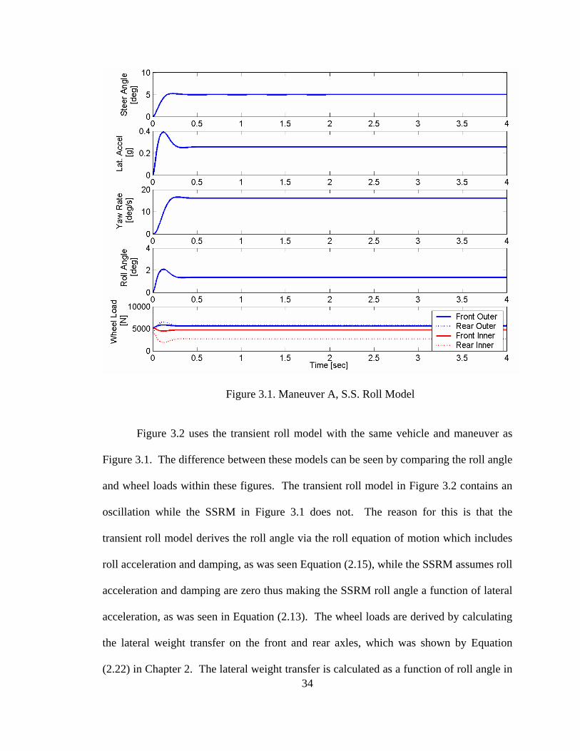
Figure 3.1. Maneuver A, S.S. Roll Model

Figure 3.2 uses the transient roll model with the same vehicle and maneuver as

Figure 3.1. The difference between these models can be seen by comparing the roll angle

and wheel loads within these figures. The transient roll model in Figure 3.2 contains an

oscillation while the SSRM in Figure 3.1 does not. The reason for this is that the

transient roll model derives the roll angle via the roll equation of motion which includes

roll acceleration and damping, as was seen Equation (2.15), while the SSRM assumes roll

acceleration and damping are zero thus making the SSRM roll angle a function of lateral

acceleration, as was seen in Equation (2.13). The wheel loads are derived by calculating

the lateral weight transfer on the front and rear axles, which was shown by Equation

(2.22) in Chapter 2. The lateral weight transfer is calculated as a function of roll angle in

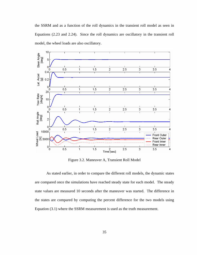
35

the SSRM and as a function of the roll dynamics in the transient roll model as seen in

Equations (2.23 and 2.24). Since the roll dynamics are oscillatory in the transient roll

model, the wheel loads are also oscillatory.

Figure 3.2. Maneuver A, Transient Roll Model

As stated earlier, in order to compare the different roll models, the dynamic states

are compared once the simulations have reached steady state for each model. The steady

state values are measured 10 seconds after the maneuver was started. The difference in

the states are compared by computing the percent difference for the two models using

Equation (3.1) where the SSRM measurement is used as the truth measurement.

36

100% Roll SS

RollTransient - Roll SS DifferencePercent ×=

3.1

Table 3.1 contains the steady state results for maneuver A. There is no wheel lift

during this maneuver, and the steady state dynamic values for the two models are

approximately the same as seen by the low percent difference between the two.

Table 3.1. Comparison of Models for Maneuver A

Dynamic State S.S. Roll Trans. Roll % Difference Units

Lateral Acceleration .2554118 .2554118 0.0 [g]

Roll Angle 1.419507 1.419058 .0316307 [deg]

Side Slip 2.278848 2.278849 .0000439 [deg]

Yaw Rate 16.09942 16.09941 .0000621 [deg/s]

Front Weight Transfer 526.9914 526.3616 .1195085 [N]

Rear Weight Transfer 1,421.585 1,421.087 .0350313 [N]

Front Lateral Force 2,650.778 2,650.778 0.0 [N]

Rear Lateral Force 2,137.870 2,137.869 .0000468 [N]

Roll Rate 5.557720 5.55596 .0316676 [deg/g]

For the next test, the step steer of 5 degrees filtered at 1.5 Hz is used again.

However, in this simulation (Maneuver B), the velocity is increased to 35 MPH. In this

input scenario, the inside rear tire in both models lifts and remains un-weighted as the

states are measured at the 10 second time interval. Figures 3.3 and 3.4 contain the

response of the SSRM and the transient roll model, respectively, during maneuver B. In

Figures 3.3 and 3.4, the rear inside wheel load is indicated by the dotted line. It is clear

that the wheel load for this tire goes to zero, which indicated wheel lift.

37

Figure 3.3. Maneuver B, S.S. Roll Model

38

Figure 3.4. Maneuver B, Transient Roll Model

The comparison of the models’ steady state dynamic states for maneuver B is

recorded in Table 3.2.

39

Table 3.2. Comparison of Models for Maneuver B

Dynamic State SS Roll Trans. Roll % Difference Units

Lateral Acceleration .8498721 .8499465 .008754 [g]

Roll Angle 4.723351 4.707426 .337154 [deg]

Side Slip -54.79752 -54.74284 .099785 [deg]

Yaw Rate 56.05783 56.03894 .033697 [deg/s]

Front Weight Transfer 1,751.426 1,728.569 1.30505 [N]

Rear Weight Transfer 4,185.143 4,185.143 0 [N]

Front Lateral Force 8,894.704 8,895.999 .014559 [N]

Rear Lateral Force 7,040.835 7,040.957 .001733 [N]

Roll Rate 5.55772 5.538496 .345897 [deg/g]

Rear Inner Wheel Lift time .373 .214 42.6273 [sec]

By examining Table 3.2, the greatest discrepancy between the two models is the

time at which the rear inner wheel lifts. However, even during this maneuver, the percent

difference between the two models is small enough that the models are still very

comparable.

The SSRM takes an additional 0.159 seconds than the transient roll model to lift

the inside rear wheel. This is explained by investigating the rear lateral weight transfer

equation which dictates the rear wheel loads. Equation (3.2) describes the general weight

transfer, while Equation (3.3) describes the full weight transfer for the rear axle.

[ ] [ ]NFFdF zizoz ⋅−= 3.2

( )[ ] [ ]NhFhhRFSFSMtrk

dF cgmyrcgmrcryrbrbrkrkrarbrr

zr ⋅⋅+−⋅+⋅+⋅+⋅= 2

3.3

40

where:

Fbr Rear damper force hrcr Rear roll center height

Fkr Rear spring force Marbr Rear anti-roll bar moment

Fyr Rear axle lateral force Ryr Reaction force on the rear

Fzi Axle inside tire wheel load Sbr Length between rear shocks

Fzo Axle outside tire wheel load Skr Length between rear springs

hcgm Un-sprung mass CG height trkr Rear track width

The lateral weight transfer equation, Equation (3.2), is calculated as the difference

between inside and outside wheel loads on each axle. An increase in the rear, lateral

weight transfer, dFzr, causes a decrease in wheel load on the rear inside tire. For this

simulation, the maximum value of dFzr is one half of the weight on the rear axle, and at

this maximum value, the rear inside wheel load is zero. The lateral weight transfer

equation is identical for both roll models; however, the rear damper force (Fbr) is zero in

the SSRM, while it has a value in the transient roll model. The rear damper force is a

function of roll velocity and the longitudinal distance between the CG and where the

damper connects to the sprung mass (Sbr). brS and Fbr are the variables in roll damping

moment (RDM), as seen in Equation (2.19). The RDM value is positive when the roll

angle velocity is positive. Note that increasing roll angle towards the outside of the

vehicle is positive. For the step maneuver, the dFzr increases faster in the transient roll

model than in the SSRM due to the positive roll angle velocity. This causes the transient

roll model to produce a wheel lift before the SSRM.

41

It is also important to note that while the transient roll model is the first to

produce wheel lift, the wheel that lifted first, touches down again between time .515 and

.543 seconds as seen in Figure 3.5. During this time, the roll angle velocity is negative

which causes the RDM to be negative and results in the dFzr decreasing from its

maximum, thus causing touch down. Touch down does not occur with the SSRM

because the roll dynamics are neglected. Therefore, once wheel lift occurs in this model,

it does not regain normal wheel load.

Figure 3.5. Zoom-In View of Test 2 Transient Model Wheel Load Response

With the minimal percent difference between the two models in the two

maneuvers found in Tables 3.1 and 3.2, the transient roll is considered accurate at steady

42

state for the dynamic states analyzed. Although, this analysis of the SSRM and the

transient roll model is successful in capturing the steady state response of the transient

roll model, further analysis of the transient model is needed to verify the full transient

response of the model.

3.3 NHTSA Phase IV Comparison

Due to the increasing fatality rate caused by rollover crashes (especially in SUVs)

Congress charged NHTSA to conduct dynamic rollover resistance rating tests. For the

purposes of a dynamic rollover resistance rating test, NHTSA selected the Fishhook

steering maneuver as a primary candidate, which was refined in the Phase IV of the

TREAD act investigation. During the TREAD act, NHTSA took exhaustive data

measurements of the vehicle dynamics from the vehicles they tested. This data was made

available to the general public and is used in this chapter to further validate the vehicle

model.

In order to validate the vehicle model described in Chapter 2, simulation results

were compared to the NHTSA Phase IV experimental data for the Fishhook 1a maneuver

(also known as the Fixed Timing Fishhook). The Fishhook 1a maneuver uses a steering

input consisting of an initial steer followed by a counter steer at a set entrance velocity.

The velocity profile of this maneuver is characterized by the vehicle reaching a desired

steady state speed, known as the entrance speed, and coasting through the rest of the

43

maneuver once the initial steer is begun. The steer angle input for the Fishhook 1a

maneuver is shown in Figure 3.6. The steer angle initially starts at zero degrees and then

commanded to steer angle ‘A’ at a rate of 720 degrees per second at the hand wheel. In

the Fishhook 1a maneuver, the steer angle ‘A’ is held constant for 0.250 seconds then a

counter steer to ‘-A’ at the same rate occurs. The steer angle ‘-A’ is held constant for 3

seconds, after which it returns to zero, completing the maneuver. The value ‘A’ is

specific to each vehicle configuration, and is defined by multiplying 6.5 by the steer

angle of the handwheel at which the vehicle experiences 0.3 g of lateral acceleration in

the Slowly Increasing Steer (SIS) maneuver. The SIS maneuver is performed at a

constant velocity of 50 mph with a continually increasing steer input of 13.5 degrees per

second at the hand wheel.

Figure 3.6. Steer Angle Input for the Fishhook 1a Maneuver

44

To accurately simulate the vehicle, there are three parameters of the Blazer that

must be quantified. These parameters are the suspension stiffness, damping, and the

front-to-rear roll stiffness ratio. However, ranges for these values are known. Therefore

a method to approximate a value for each of these properties without ‘tuning’ the

properties for a specific maneuver was used. NHTSA evaluated the Blazer using

multiple maneuvers such as the J-Turn, Fishhook 1a, and Fishhook 1b. Since the

maneuver of most dynamic interest, the Fishhook 1a, is used later for model validation,

the J-Turn maneuver is compared with the simulation in order to back out the

approximate unknown properties. The frequency and damping of the suspension’s roll

dynamics are seen in the roll data in Figure 3.7. With this information, the suspension

roll stiffness and roll damping are varied to match the roll angle frequency and damping.

Since the differences between the front and rear roll stiffness and roll damping are not

known at this point, they are kept equal to one another.

45

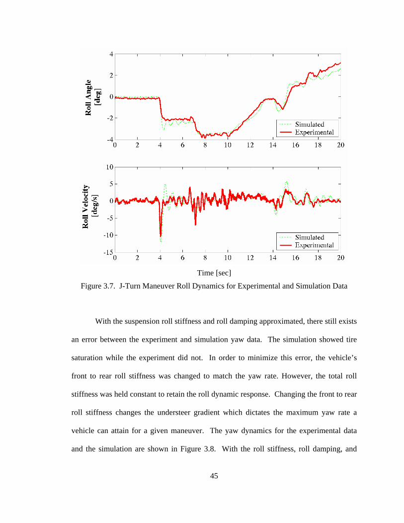
Time [sec]

Figure 3.7. J-Turn Maneuver Roll Dynamics for Experimental and Simulation Data

With the suspension roll stiffness and roll damping approximated, there still exists

an error between the experiment and simulation yaw data. The simulation showed tire

saturation while the experiment did not. In order to minimize this error, the vehicle’s

front to rear roll stiffness was changed to match the yaw rate. However, the total roll

stiffness was held constant to retain the roll dynamic response. Changing the front to rear

roll stiffness changes the understeer gradient which dictates the maximum yaw rate a

vehicle can attain for a given maneuver. The yaw dynamics for the experimental data

and the simulation are shown in Figure 3.8. With the roll stiffness, roll damping, and

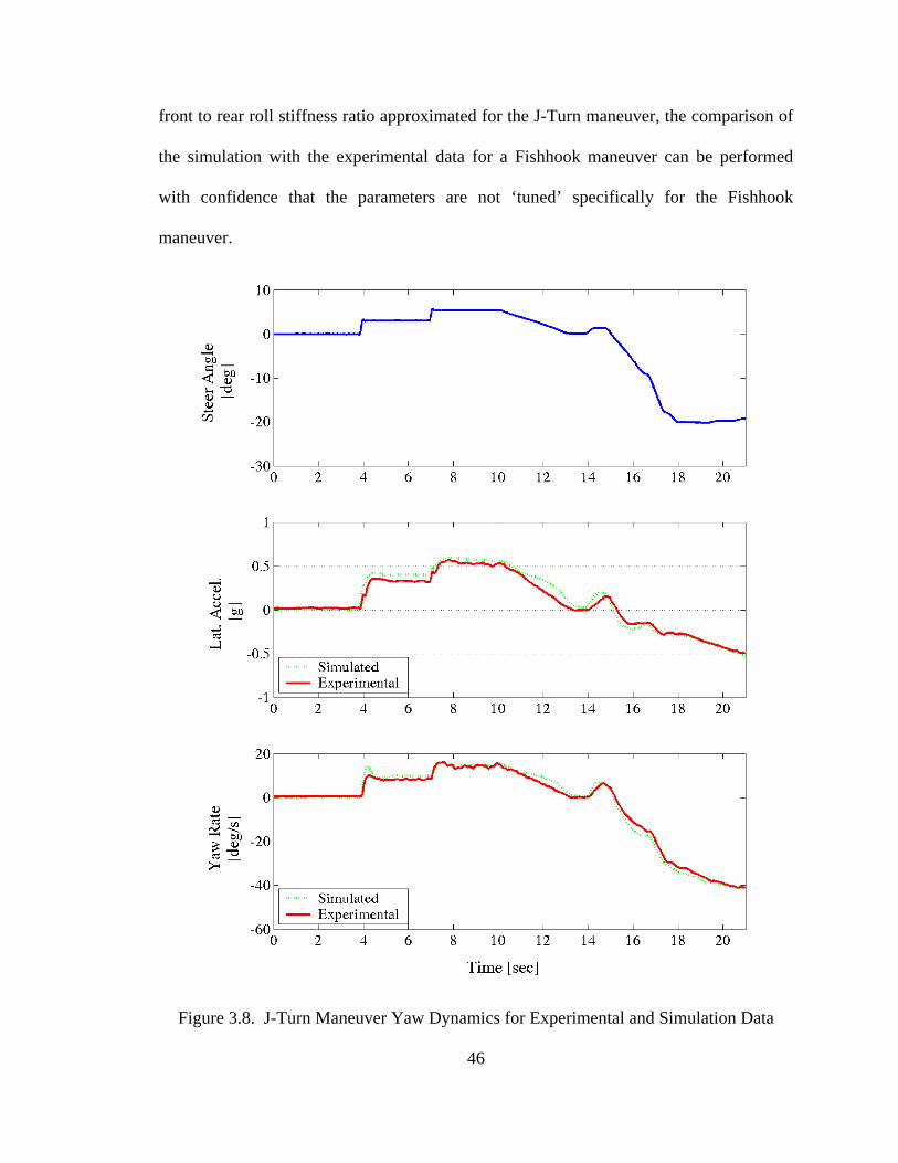
46

front to rear roll stiffness ratio approximated for the J-Turn maneuver, the comparison of

the simulation with the experimental data for a Fishhook maneuver can be performed

with confidence that the parameters are not ‘tuned’ specifically for the Fishhook

maneuver.

Figure 3.8. J-Turn Maneuver Yaw Dynamics for Experimental and Simulation Data

47

The vehicle used for comparison in this study is a 2001 Chevy Blazer 4x2.

NHTSA’s Phase IV experiments recorded data for the Blazer in three different

configurations: Nominal, Reduced Rollover Resistance (RRR), and Rear Mounted Ballast

(RMB). The Nominal configuration is the Blazer equipped with a driver, data

acquisition, and outriggers on board. It has a weight distribution of 55:45 (front to rear),

CG height of 26.3 inches, and a track width of 56.89 inches. These parameters result in a

static stability factor (SSF) of 1.048 (Equation 1.1). Complete property values of each

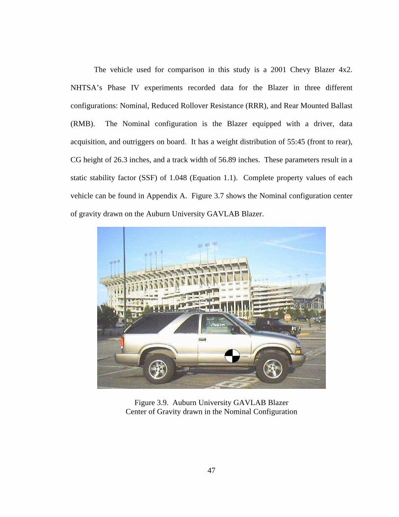
vehicle can be found in Appendix A. Figure 3.7 shows the Nominal configuration center

of gravity drawn on the Auburn University GAVLAB Blazer.

Figure 3.9. Auburn University GAVLAB Blazer Center of Gravity drawn in the Nominal Configuration

48

Figure 3.10 shows the Nominal Blazer experimental data and simulation data

during a Fishhook 1a maneuver. Both the yaw and roll dynamics of the transient yaw

and roll model closely match to dynamic states measured in the actual vehicle.

Figure 3.10. Nominal Blazer Dynamics for a Fishhook 1a Maneuver

49

The RRR configuration is the vehicle in the Nominal configuration with a 181 lbs

roof ballast added on the top of the vehicle and shown in Figure 3.11. This serves to raise

the CG vertically by 5% from the Nominal configuration to 27.6 inches. This results in a

new SSF of 0.989, while maintaining the same vehicle longitudinal weight split as the

Nominal configuration.

Figure 3.11. Auburn University GAVLAB Blazer Center of Gravity drawn in the RRR Configuration

In order to conduct this simulation, the CG height, roll inertia, and yaw rate were

the only parameters that were changed in the garage when converting the Nominal Blazer

to the RRR Blazer. The changes of these properties were recorded in the NHTSA study

and are shown in Table 3.3.

Table 3.3. Nominal vs. RRR Blazer Configuration [Forkenbrock, 2002]

Weight (lbs)

CG Height (inches)

Roll Inertia (ft-lbs-sec2)

Yaw Inertia (ft-lbs-sec2)

Pitch Inertia (ft-lbs-sec2)

Nom. Blazer 4154 26.3 520 2765 2573 RRR Blazer 4335 27.6 579 2766 2637

50

The roll inertia for the RRR configuration is 11.3 percent higher than the Nominal

configuration. However, since the placement of the roof ballast is near the CG in the x

and y axes, the yaw inertia changes by less than 0.04 percent. Though pitch inertia is

neglected in vehicle model, thus not needed, it is interesting to note the roof mounted

ballast causes it to increase by 2.49 percent. The increase in the pitch inertia will cause

an increase in understeer during heavy breaking with the Blazer.

In Figure 3.12, the experimental and simulated RRR Blazer configuration data is

compared. Again, the vehicle model follows the actual RRR Blazer Fishhook 1a

experiment data. The largest discrepancy between the simulation and experimental data

is in the roll angle. This is most likely due to wheel lift of the inside tires.

51

Figure 3.12. RRR Configuration Blazer Dynamics for a Fishhook 1a Maneuver

The RMB configuration is the vehicle in the Nominal configuration with weight

added to the rear of the vehicle, which moves the CG longitudinally by 10.5 inches

toward the rear, but retains the same SSF. This center of gravity shift is illustrated in

Figure 3.13. The RMB has a front to rear weight distribution of 44:56, but maintains the

SSF of 1.048. For the Nominal and RRR configurations, experimental data for a

52

Fishhook 1a maneuver is available. However, for the RMB configuration, only

experimental data for a Fishhook 1b maneuver is available. The Fishhook 1b maneuver is

similar to the Fishhook 1a, but does have some subtle differences [Forkenbrock, 2002;

NHTSA, 2002].

Figure 3.13. Auburn University GAVLAB Blazer Center of Gravity drawn in the RMB Configuration

Table 3.4 reveals the change in vehicle properties between the Nominal and RMB

Blazer configurations.

Table 3.4. Nominal vs. RMB Blazer Configuration [Forkenbrock, 2002]

Weight Split Front:Rear

CG Height (inches)

Roll Inertia (ft-lbs-sec2)

Yaw Inertia (ft-lbs-sec2)

Pitch Inertia (ft-lbs-sec2)

Nom. Blazer 55:45 26.3 520 2765 2573 RMB Blazer 44:56 26.1 567.9 3604 3368.3

53

Figure 3.14. RMB Configuration Blazer Dynamics for a Fishhook 1b Maneuver

Figure 3.14 shows experimental and simulation results from Fishhook 1b for the

RMB configuration. The largest discrepancy between the simulation results and the

experiment data is again in the roll angle. The experimental data reveals that two-wheel

lift occurs. This is seen in the roll angle measurement along with the NHTSA notes for

54

this experiment. However, the simulation result predicts only one-wheel lift with the

second wheel approaching wheel lift. This is seen from the normal forces for each tire, as

shown in Figure 3.15. This difference is most likely due to limitations of the simulation

model. Some of the model’s assumptions discussed in Chapter 2 may not be valid for all

scenarios the vehicle encounters. For example, the roll stiffness is more than likely not

linear in the real Blazer. Also, the assumption of the un-sprung mass being in steady

state is no longer accurate after one wheel lift occurs for the roll dynamics (yet it appears

to remain valid for the yaw dynamics). Also note that this discrepancy is small and it

occurs only in the Fishhook 1b RMB data.

55

Figure 3.15. RMB Configuration Blazer Wheel Loads for a Fishhook 1b Maneuver

56

3.4 Auburn University GAVLAB Blazer

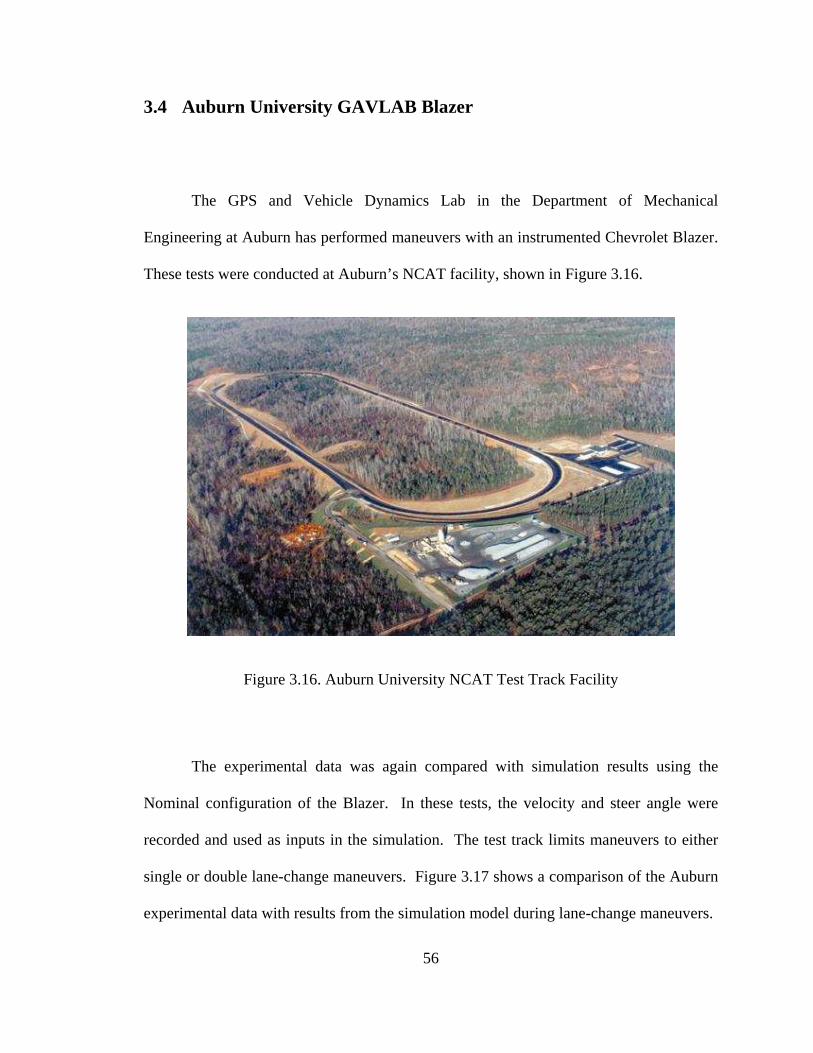
The GPS and Vehicle Dynamics Lab in the Department of Mechanical

Engineering at Auburn has performed maneuvers with an instrumented Chevrolet Blazer.

These tests were conducted at Auburn’s NCAT facility, shown in Figure 3.16.

Figure 3.16. Auburn University NCAT Test Track Facility

The experimental data was again compared with simulation results using the

Nominal configuration of the Blazer. In these tests, the velocity and steer angle were

recorded and used as inputs in the simulation. The test track limits maneuvers to either

single or double lane-change maneuvers. Figure 3.17 shows a comparison of the Auburn

experimental data with results from the simulation model during lane-change maneuvers.

57

Time (sec)

Figure 3.17. Lane Change Maneuver Data for the GAVLAB Blazer

Though the yaw dynamics of the experiment and simulation data closely match

each other, differences between the simulation and experiment roll angles can be clearly

seen in Figure 3.18. This is caused by a change in the bank angle of 4 degrees during the

lane change maneuver, commonly known as the road crown (which aids in water

drainage).

58

Figure 3.18. Lane Change Maneuver Yaw and Roll Angle Data for the GAVLAB Blazer

The parameters used in this simulation are the ones used for the Nominal Blazer

which were tuned with the NHTSA experimental data for the J-Turn maneuver. The

similarity of the dynamic behavior in the simulation and the various experiments provide

much confidence in the vehicle model.

59

3.5 Lateral Weight Transfer Simulation

In the some of the simulation maneuvers, the vehicle exhibits an initial counter

weight transfer, analogous to a non-minimum phase system. In other words, during a

maneuver, the weight transfer is initially in opposite direction of steady state weight

transfer as seen in Figure 3.5. The steady state values for the dynamic states reveal that

the outside wheel loads are higher than the inside wheel loads, as seen in Figure 3.4.

However, at the beginning of a step maneuver, the front inside wheel load increases and

the front outside decreases, as seen in Figure 3.5. Closer analysis shows that during the

first 0.1685 seconds of the maneuver the weight transfer on the front axle is negative.

This increases the inside wheel load. For the normal force on the inside wheel to increase

during a turn is counter intuitive. In steady state, the normal force on an axle’s inside

wheel decreases and the normal force on the outside wheel of the same axle increases as

expected.

In order to understand this phenomenon, the weight transfer equation must be

further examined. The weight transfer equation for the front axle and rear axle are the

same. However, vehicle parameters for the front and rear axles are different. The

equation of the front weight transfer from Chapter 2 is shown again here as Equation

(3.4).

( )[ ] [ ]NhFhhRFSFSMtrk

dF cgmyfcgmrcfyfbfbfkfkfarbff

zf ⋅⋅+−⋅+⋅+⋅+⋅= 2

3.4

60

During the initial 0.1685 seconds of the step maneuver, the roll angle and velocity

are positive and therefore the moments from the anti-roll bar ( arbfM ), springs ( kfkf FS ⋅ )

and dampers ( bfbf FS ⋅ ) are all positive. By investigating the un-sprung mass free body

diagram in Figure 3.19, it is seen that the tire lateral forces are also positive for this left

steer, step steer maneuver.

Figure 3.19. Roll FBD Un-Sprung Mass

The only variable remaining in the weight transfer equation that could be negative

and cause dFzf to be negative is the term ( )cgmrcfyf hhR −⋅ . For the step maneuver, the

lateral reaction force is always positive. Therefore, the variables causing the initial

counter weight transfer are the un-sprung mass CG height and the roll center height.

When the roll center height is below the un-sprung mass CG height, the moment arm

becomes negative and is multiplied by a positive lateral reaction force, thus causing the

Fyi

Fzi

Fzo

Ry

Rz

rc

CGm

Fbi + Fki

Fbo + Fko

mg

Inside

Outside

Fyo

S/2

trk

Marb

61

dFzf to be negative at the beginning of this maneuver. On the Blazer vehicle model, the

front roll center height is below the un-sprung mass CG height and the rear un-sprung

mass height is equal to the un-sprung mass height. Because the rear weight transfer is

never negative, note that the inside rear wheel load is never greater than the outside rear

in Figure 3.5. This is due to the fact that the un-sprung mass CG height and the roll

center height are the same; the moment arm of the ( )cgmrcfyf hhR −⋅ term is zero.

To clarify which variable or variables is causing the weight transfer to be negative, three

terms of the front lateral weight transfer are analyzed separately. These terms include the

total front weight transfer, the front weight transfer without the ( )cgmrcfyff

hhRtrk

−⋅⋅2

term, and the ( )cgmrcfyff

hhRtrk

−⋅⋅2 term. Figure 3.16 shows these terms during a step

maneuver.

62

Figure 3.20. Maneuver B, Transient Roll, Front Lateral Weight Transfer

It can see in Figure 3.20 that the dFzf is negative before time 0.1685 seconds.

This is because the Ryf component is greater than the other terms of Equation (3.4). This

narrows the possible vehicle properties that cause the counter weight transfer down to

two: the roll center height and the un-sprung mass CG height.

To further explore the counter weight transfer on the front axle, a simulation of a

step steer input is performed with both front and rear roll center heights equal to the un-

sprung mass CG height. The response is shown in Figure 3.21.

63

Figure 3.21. Step Maneuver with Roll Center Height equal to Un-Sprung Mass CG Height

It is shown that the counter weight transfer does not exist when the roll center

height is equal to the un-sprung mass CG height. Also note the convention of the

negative tire slip angles producing positive lateral tire forces. The conclusion is that a

roll center height below the un-sprung mass CG height creates an initial counter weight

transfer.

64


In this chapter, the accuracy and validity of the transient roll model has been

demonstrated. The transient roll model was shown to produce the same steady state

results as the steady state roll model. Experimental vehicle data acquired from NHTSA’s

Phase IV rollover research was used to determine unknown vehicle properties.

Additional data from the Phase IV testing was then used to validate that the transient roll

model matches the transient dynamics of the experimental data. It has also been shown

that the vehicle model accurately captures the dynamics of the vehicle when properties

are changed, as shown by the RRR and RMB Blazer configurations. Experimental data

produced by the Auburn University GAVLAB was used to provide further validation that

the vehicle model matches experimental data for a lane change maneuver. An initial

counter weight transfer was seen in the wheel load data during the simulation maneuvers.

This phenomenon was examined and ultimately produced more confidence in the

simulation’s accuracy. This wide range of validation of the model developed in Chapter

2 allows for confidence in the vehicle dynamics analysis in the following chapters.

65

CHAPTER 4

ANALYSIS OF VEHICLE ROLLOVER STABILITY LIMIT

4.1 Introduction

This chapter investigates the effect of various vehicle parameters on rollover

propensity using computer simulation. The vehicle model used in the simulation was

developed in Chapter 2. The computer simulation’s accuracy was verified in Chapter 3

by comparing the simulation data to experimental data from NHTSA’s Phase IV testing

on rollover of passenger vehicles. In this chapter, the vehicle model is subjected to a

specific steering input defined by NHTSA, called the Fishhook 1a. An analysis of the

vehicle loading condition and its influence on rollover propensity is conducted using the

validated vehicle simulation.

66

4.2 NHTSA Phase IV Analysis

As discussed previously, NHTSA performed the Phase IV of TREAD rollover

analysis in 2002. Chapter 3 showed data for a 2001 Blazer in various configurations that

were tested, and this data was used to validate the vehicle simulation. In the NHTSA

tests, the vehicle’s loading condition was changed to three specific locations. The

Nominal, Reduced Rollover Resistance (RRR), and Rear Mounted Ballast (RMB)

configurations represent these loading condition changes, which are shown in Table 4.1.

Table 4.1. NHTSA Phase IV Vehicle Load Configurations [Forkenbrock, 2002]

Nominal RRR RMB CG Height [inches] 26.3 27.6 26.1 Weight Split Front : Rear

55:45 55:45 44:56

NHTSA performed a Fishhook 1b maneuver with the Blazer in each of these

configurations. To determine vehicle rollover, the Blazer was equipped with outriggers

to allow the vehicle to lift both wheels of one side of the vehicle. Entrance speeds of the

maneuver were increased until two-wheel-lift (TWL) was detected. TWL was defined as

both wheels on one side of the vehicle being two inches off the ground. Table 4.2

contains the NHTSA Phase IV data which shows the Blazer lowest entrance speed at

which TWL was detected.

Table 4.2. Blazer TWL Velocity in Fishhook 1b Maneuver [Forkenbrock, 2002]

Nominal RRR RMB TWL Velocity [mph] 40.1 36.2 34.9

67

The results of this experiment show that the Blazer’s tendency to rollover

increases as the CG height is increased. The RRR configuration has a CG height 1.3

inches higher than the Nominal configuration and experiences TWL at 36.2 mph while

the Nominal configuration requires 3.9 mph more velocity before TWL is achieved. This

follows intuition and the results of the SSF explained previously.

The RMB configuration, like the RRR, increases the Blazer’s tendency to

rollover. However, the CG height of the RMB is 0.2 inches lower than the Nominal CG

height. The physical difference between these two configurations causing the TWL

velocity variation is the weight split. The Nominal and RMB have approximately the

same SSF, and weight splits of 55:45 and 44:56, respectively. NHTSA performed a

Fishhook 1b maneuver on both of these configurations, and the Nominal configuration

experienced TWL at 40.2 mph, while the RMB had TWL at 34.9 mph.

In order to better quantify the difference between the Nominal and RMB

configurations, the vehicle model is used to simulate and duplicate NHTSA’s Phase IV

data for the Blazer. The vehicle’s weight split and CG height are varied to assess their

affect on rollover propensity. The front to rear weight split is varied from 30:70 to 70:30,

while holding the SSF constant. The Nominal configuration of the Blazer is also

modified so that the roll center, suspension stiffness and damping are the same on the

front and rear. With these changes to the suspension, the effects of changing the weight

split are isolated from other factors. The parameters varied in this simulation test are the

lengths ‘a’ and ‘b’, while their sum, the wheelbase, is held constant. The Slowly

Increasing Steer (SIS) maneuver and constant are used and adopted from the NHTSA

Fishhook 1a test. The change in weight distribution caused the SIS constant to also

68

change for each different weight split. For each parametric variation of the vehicle load

condition, a new SIS constant is determined as described in Chapter 3. The SIS constant

varied from 0.675 to 1.827 degrees at the tire for the splits of 30:70 to 70:30 respectively

as shown in Figure 4.1.

0.50

0.75

1.00

1.25

1.50

1.75

2.00

30 40 50 60 70

Percent Weight on the Rear Axle

SIS

Co

nsta

nt [

deg

]

Figure 4.1. SIS Constant Change for Weight Split Variation

The dynamic test used to determine the effects of these property changes is the

Fishhook 1a maneuver. The Fishhook 1a is a highly repeatable maneuver as cited by

NHTSA’s Phase IV research and is an easily programmed open loop input (unlike its the

Fishhook 1b, which requires roll velocity data in a closed loop feedback control)

[Forkenbrock, 2003].

As in the NHTSA study, rollover velocity is calculated by determining the vehicle

speed at which the steering maneuver causes TWL. As previously described, NHTSA

determines TWL as both wheels on one side of the vehicle being lifted 2 inches off the

69

ground. However, TWL for the simulation is defined as the instant that the normal forces

on both tires on one side of the vehicle go to zero. This definition is due to the fact that

the simulation is not able to measure the height of each wheel after wheel lift since the

un-sprung mass dynamics are not modeled. The simulation is still accurate until the point

where wheel lift occurs. The difference in the definition of TWL between the simulation

and experiment results in a discrepancy in the velocity that TWL occurs. Since the

simulation rollover is defined as the instant that TWL occurs and not after both wheels

have lifted 2 inches, the rollover velocity for the simulation is lower than the NHTSA

experiment data. Figure 4.2 shows the simulation of TWL velocity across a range of

vehicle weight splits. NHTSA’s Nominal and RMB configurations for the Blazer are

also shown in Figure 4.2.

25

30

35

40

45

50

30 40 50 60 70Percent Weight on the Rear Axle

TW

L V

elo

city

[m

ph

]

Simulation

NHTSA NominalConfiguration

NHTSA RMBConfiguration

Figure 4.2. TWL Velocity for Weight Split Variation

70

Figure 4.3 shows the corresponding understeer curve. Inspection of Figures 4.2

and 4.3 reveals a correlation between understeer and rollover propensity. As the Blazer’s

weight is shifted toward the rear, the vehicle begins to oversteer as well as roll at a lower

velocity than when the weight is shifted toward the front axle. Also note that as the

weight is shifted toward the front axle, the corresponding SIS increases causing the

Fishhook 1a to become a more severe maneuver. However, the TWL velocity continues

to increase as the weight is moved to the front axle. NHTSA’s Phase IV experiments

reveal this same correlation between weight split and rollover propensity, as seen in

Figure 4.2.

Figure 4.3. Vehicle Understeer Gradient for a Variation of Weight Splits

Another interesting observation from the simulation data was seen for two vehicle

configurations with a SSF equal to 1.048. One vehicle configuration experiences TWL at

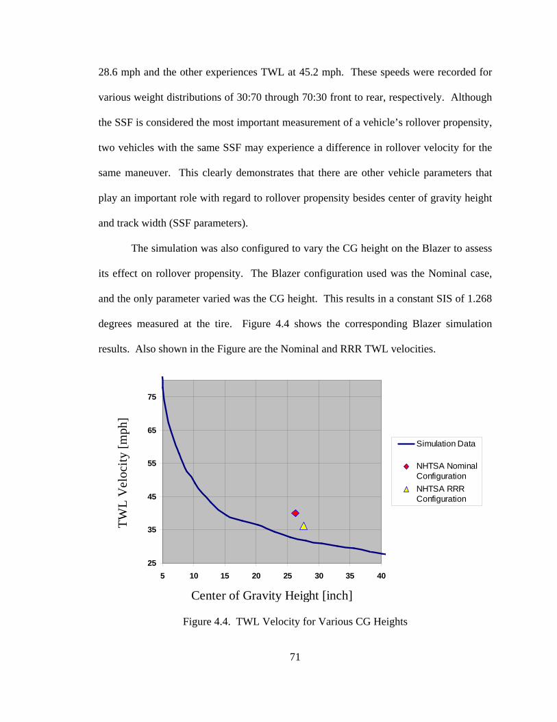
71

28.6 mph and the other experiences TWL at 45.2 mph. These speeds were recorded for

various weight distributions of 30:70 through 70:30 front to rear, respectively. Although

the SSF is considered the most important measurement of a vehicle’s rollover propensity,

two vehicles with the same SSF may experience a difference in rollover velocity for the

same maneuver. This clearly demonstrates that there are other vehicle parameters that

play an important role with regard to rollover propensity besides center of gravity height

and track width (SSF parameters).

The simulation was also configured to vary the CG height on the Blazer to assess

its effect on rollover propensity. The Blazer configuration used was the Nominal case,

and the only parameter varied was the CG height. This results in a constant SIS of 1.268

degrees measured at the tire. Figure 4.4 shows the corresponding Blazer simulation

results. Also shown in the Figure are the Nominal and RRR TWL velocities.

25

35

45

55

65

75

5 10 15 20 25 30 35 40

Center of Gravity Height [inch]

TW

L V

elo

city

[mph

]

Simulation Data

NHTSA NominalConfiguration

NHTSA RRRConfiguration

Figure 4.4. TWL Velocity for Various CG Heights

72

With the track width is held constant, the SSF varies from 3.467 to 0.2774 with

change in CG height. The Nominal configuration has a SSF of 1.048, which corresponds

to a CG height of 16.76 inches. The TWL velocity for the Nominal configuration as

determined by the simulation is 38.8 mph. NHTSA documented TWL for the same

configuration and maneuver as being 40.2 mph. Again, the difference in the TWL

velocities is caused by the different definition of TWL between the simulation and

experiment. The observed trend of the data is not surprising since it is well known that a

vehicle will roll at a lower velocity if the CG is raised or the SSF is decreased.

4.3 Stability Limit Development

From Section 4.2, it can be seen that a vehicle’s rollover threshold varies not only

with CG height, but also the CG longitudinal location, otherwise known as the vehicle’s

weight split. In this section, vehicle states other than rollover velocity are measured to

further develop an understanding of how the vehicle’s dynamic states at rollover vary

with the vehicle’s load condition.

Vehicle simulations are again used to determine the stability threshold for

different vehicle load conditions. This is done by independently varying the vehicle’s

center of gravity height and weight split. The maximum value of the each of the

following states is recorded when rollover is detected: maneuver entrance velocity, lateral

acceleration, yaw rate, roll angle, roll rate, side slip angle, and side slip rate. For the

general Fishhook maneuver, rollover is consistently measured slightly after the maximum

73

counter steer. The Fishhook maneuver used is different than the NHTSA Fishhook 1a

because the maneuver’s steer angle magnitude is independent of the SIS constant

described in Chapter 3. Therefore, the maneuver is unchanged for variations of vehicle

properties, thus allowing for a more concise comparison between the property variations.

For these simulations, a Fishhook steering profile was chosen with a maximum

steer angle of 5 degrees and a maximum steering rate of 40 deg/s, both measured at the

tires. This profile was filtered by a second order 0.75 Hz Butterworth filter to remove the

abrupt changes in the simulation’s steer angle.

The first property varied was the CG height. The Nominal Blazer configuration

was used as the baseline. The CG height was varied between 65 and 160 percent of the

baseline CG height. The rollover velocity, lateral acceleration and yaw rate are shown in

Figure 4.5. As shown in the previous section, the vehicle will roll at lower velocities as

the CG height is raised. Also, note that as the CG height is raised, the lateral

acceleration and yaw rate that the vehicle can achieve before experiencing a rollover

event is decreased. These results confirm those of the SSF, which states that the vehicle

is more prone to rollover as the CG height is increased.

74

Figure 4.5. Velocity and Yaw Dynamics at Rollover for CG Height Variation

The roll angle and roll rate along with the side slip angle and the side slip rate are

important states when determining rollover [Hac, 2004]. Currently, Ford utilizes the roll

rate dynamic state in its electronic stability control system for SUVs, and much research

is ongoing to use the side slip rate state in vehicle stability control systems. The

following states at rollover are shown in Figure 4.6: roll angle, roll rate, side slip, and

side slip rate.

75

Figure 4.6. Roll and Side Slip States at Rollover for CG Height Variation

As the CG height is increased, the roll angle and roll rate at rollover increase.

This increase in roll angle and roll rate is caused by the increase in the vertical distance

(d1) between the roll center axis and the CG height as the CG height is raised. The angle

of roll per lateral acceleration is known as the Roll Rate property (not to be confused with

the roll rate [deg/s] state), as seen in Equation (4.1) [Gillespie, 1992] and Figure 4.7

shows the change in Roll Rate as the CG height is varied.

Roll Rate

⋅⋅

⋅⋅+−⋅⋅−

=gdgMk

dgM

t

deg180

1

1

πφ

4.1

76

Figure 4.7. Roll Rate for CG Height Variation

The lateral force on the front and rear axles for the CG height variation is shown

in Figure 4.8. It can be seen that as the CG height increases, the lateral force at vehicle

rollover is decreased.

77

Figure 4.8. Lateral Tire Force at Rollover for CG Height Variation

The second property which was varied on the Nominal Blazer is the vehicle’s

weight split. The vehicle weight split was varied from a weight ratio of 70:30 (front axle

to rear axle) to a ratio of 30:70. The same maneuver and vehicle from the CG height

variation simulation were used. Figure 4.9 shows the velocity, lateral acceleration, and

yaw rate at rollover for the weight split variation simulations.

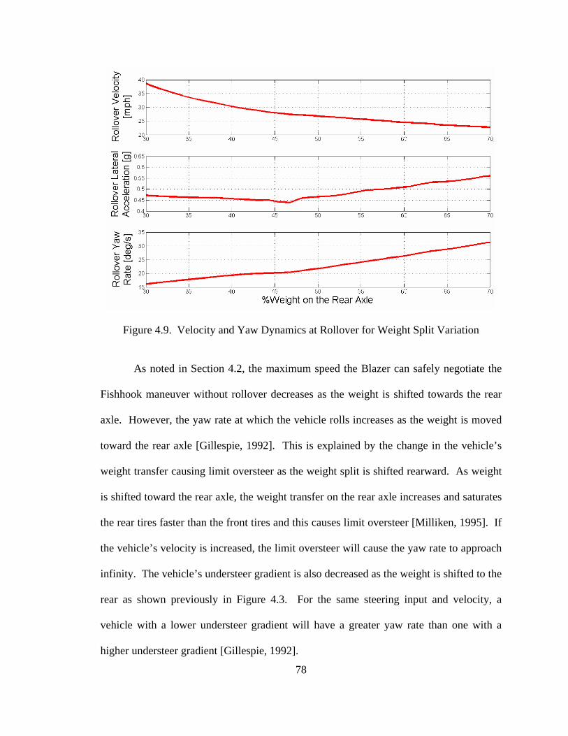
78

Figure 4.9. Velocity and Yaw Dynamics at Rollover for Weight Split Variation

As noted in Section 4.2, the maximum speed the Blazer can safely negotiate the

Fishhook maneuver without rollover decreases as the weight is shifted towards the rear

axle. However, the yaw rate at which the vehicle rolls increases as the weight is moved

toward the rear axle [Gillespie, 1992]. This is explained by the change in the vehicle’s

weight transfer causing limit oversteer as the weight split is shifted rearward. As weight

is shifted toward the rear axle, the weight transfer on the rear axle increases and saturates

the rear tires faster than the front tires and this causes limit oversteer [Milliken, 1995]. If

the vehicle’s velocity is increased, the limit oversteer will cause the yaw rate to approach

infinity. The vehicle’s understeer gradient is also decreased as the weight is shifted to the

rear as shown previously in Figure 4.3. For the same steering input and velocity, a

vehicle with a lower understeer gradient will have a greater yaw rate than one with a

higher understeer gradient [Gillespie, 1992].

79

The maximum lateral acceleration that Blazer can achieve before rollover also

increases as the weight split is moved rearward. The lateral acceleration at rollover as the

weight is shifted to the rear mimics the yaw rate at rollover. Although Equation (4.2) is

only true at steady state, it does explain why the lateral acceleration at rollover trend

follows the yaw rate at rollover trend.

2rVay ⋅= 4.2

Figure 4.10 shows the maximum roll angle, roll rate, side slip angle, and side slip

rate achieved at rollover. The rollover roll angle remains nearly constant as weight split

is varied. However, the rollover roll angle rate decreases as the vehicle’s weight is

shifted to the rear axle. The side slip rate varies from 0 to 0.5 deg/s at rollover yet the

side slip angle decreases at the weight split is shifted toward the rear.

Figure 4.10. Roll and Side Slip Thresholds for Weight Split Variation

80

4.4 Tire Property Variation

As noted in Chapter 2, the non-linear, ‘Magic Formula’ tire model can be easily

modified. In this section, the tire’s cornering stiffness and peak lateral force are varied to

see how they affect rollover propensity. Again, a Fishhook maneuver of 5 degrees is

used to study this effect.

To examine how peak lateral tire force influences rollover, three different tires

were used. The three different tires are modeled in Figure 4.11 with the tire normal

force set at 5 kN. As seen in Figure 4.11, the cornering stiffness is held constant at 2400

N/deg for each tire, but each tire has a different peak lateral force.

Figure 4.11. Tire Curves for Variation of Peak Lateral Tire Force (Fz =5 kN)

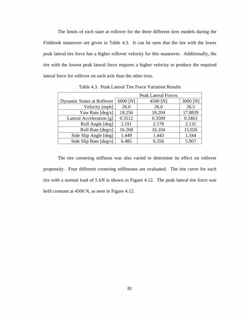
81

The limits of each state at rollover for the three different tires models during the

Fishhook maneuver are given in Table 4.3. It can be seen that the tire with the lower

peak lateral tire force has a higher rollover velocity for this maneuver. Additionally, the

tire with the lowest peak lateral force requires a higher velocity to produce the required

lateral force for rollover on each axle than the other tires.

Table 4.3. Peak Lateral Tire Force Variation Results

Peak Lateral Forces Dynamic States at Rollover 6000 [N] 4500 [N] 3000 [N]

Velocity [mph] 26.0 26.0 26.5 Yaw Rate [deg/s] 18.256 18.204 17.8839

Lateral Acceleration [g] 0.3512 0.3509 0.3463 Roll Angle [deg] 2.191 2.178 2.131 Roll Rate [deg/s] 16.268 16.104 15.026

Side Slip Angle [deg] 1.449 1.443 1.344 Side Slip Rate [deg/s] 6.485 6.356 5.907

The tire cornering stiffness was also varied to determine its effect on rollover

propensity. Four different cornering stiffnesses are evaluated. The tire curve for each

tire with a normal load of 5 kN is shown in Figure 4.12. The peak lateral tire force was

held constant at 4500 N, as seen in Figure 4.12.

82

Figure 4.12. Tire Curves for Variation of Tire Cornering Stiffness (Fz =5 kN)

The limits of each state at rollover for the tire models with the tire cornering

stiffness variation are seen in Table 4.4. The tire with the lowest cornering stiffness

requires the highest velocity in the Fishhook maneuver to rollover. The rollover velocity

is higher in the tire with the lowest cornering stiffness because a higher velocity is

required to produce the same lateral force that the other tire models rollover.

83

Table 4.4. Tire Cornering Stiffness Variation Results

Tire Cornering Stiffness [N/deg] Dynamic States at Rollover 3000 2400 1500 1000

Velocity [mph] 25.25 26.0 28.0 29.25 Yaw Rate [deg/s] 18.574 18.214 17.50 16.604

Lateral Acceleration [g] 0.3651 0.3511 0.3245 0.2934 Roll Angle [deg] 2.282 2.180 1.985 1.773 Roll Rate [deg/s] 18.801 16.154 11.523 8.1247

Side Slip Angle [deg] 1.710 1.444 0.9541 1.381 Side Slip Rate [deg/s] 7.214 6.369 4.769 5.472


In this chapter, simulation data along with NHTSA experimental data were used

to evaluate how two vehicle properties, CG height and weight split, affect a vehicle’s

rollover limit. The simulations were also used to explore how the cornering stiffness and

peak lateral force of the tire affect a vehicle’s rollover propensity. It was shown that the

SSF is not the sole determinate of a vehicle’s rollover propensity, and that there are

vehicle properties other than SSF, such as weight distribution and tire properties, that can

significantly influence rollover propensity. It was also shown that there is a correlation

between the understeer gradient and rollover propensity. As the vehicle understeer

increases, the TWL velocity tends to increase.

Finally, rollover stability limits were developed in this chapter. The stability

threshold consisted of many vehicle dynamics states: velocity, lateral acceleration, yaw

84

rate, roll angle, roll angle rate, side slip angle, and side slip rate. Those were the states

used to express the rollover stability limits. These stability limits will be used with an

ESC in the following chapters.

86

CHAPTER 5

ELECTRONIC STABILITY CONTROL DEVELOPMENT

5.1 Introduction

As was stated in Chapter 1, vehicle rollover accidents have received much

attention in the past decade. There is high demand for SUVs (vehicles with low SSFs) in

the automobile market despite their high rollover propensity. The automotive

engineering world’s solution to making these vehicles safer is electronic stability control

(ESC). As was shown in the previous chapters, the foundation of ESC begins with an

understanding of how vehicle dynamics and vehicle properties affect rollover. These

principles are used to develop the stability controller in this chapter.

The first generation ESCs implemented yaw control by limiting yaw rates with

differential braking [Tseng, 1999]. These ESCs used yaw rate gyros, wheel speed

sensors, and lateral accelerometers and the pre-existing anti-lock braking actuator.

Although differential braking is still the most common actuator used in ESCs, others such

as active suspensions and steer-by-wire, are being developed to enter the market

[Vilaplana, 2004; Amberkar, 2004]. Although yaw control has been shown to reduce

rollover, Ford utilizes an ESC that couples the yaw and roll dynamics for control and

therefore equips their SUVs with a roll rate gyro [van Zanten, 2000].

87

In this chapter, a simple ESC is developed and implemented on a Blazer in

simulation. It uses steer angle and braking to control the vehicle’s stability and to track

the driver’s intended path.

5.2 Electronic Stability Control

The ESC developed and used in this thesis is a proportional and integral (PI) yaw

controller. It uses the vehicle’s brakes to control velocity and controls the steer angle of

the front tires. Controller limits are given from the stability threshold derived in Chapter

4. The ESC takes these limits into account and adjusts the steer angle and velocity to

keep the vehicle within the stability region.

In order to implement the P-I controller, the vehicle model must first be

linearized. Placing the linearized equation of the bicycle model into the state space form

is shown in Equation (5.1).

[ ]δββ

α

α

⋅

⋅⋅+

⋅

⋅−−

−⋅

−⋅

−

=

z

f

f

zz I

CaVMT

C

rVI

C

I

CVMT

C

VMT

C

r 32

221 1

&

&

5.1

Equations (5.2 – 5.4) provide the definitions of the constants C1, C2, and C3.

raaf CCC +=1 5.2

88

araf CbCaC ⋅−⋅=2 5.3

araf CbCaC ⋅+⋅= 223 5.4

The tire cornering stiffnesses fCα and rCα represent the total axle cornering

stiffness of the front and rear axles, respectively. The axle cornering stiffness is found by

adding the cornering stiffness of each tire for that axle.

The yaw dynamics are controlled with a PI controller. The transfer function for

the PI controller is given in Equation (5.5).

s

ksk

Input

Output ip +⋅=

5.5

Where:

kp = Proportional Gain

ki = Integral Gain

The controller gains were chosen by imputing the desired response frequency of 1

Hz and desired damping of 0.707 into the MATLAB ‘place’ command. The ‘place’

command sets the controller’s eigenvalues to achieve the desired output. The

proportional gain was 1.0, and the integral gain was -0.5.

The Nominal Blazer configuration is simulated with and without the ESC

activated. The Fishhook 1a steering profile is once again used. The maneuver velocity

was set at 35 mph, yet the vehicle can only negotiate this maneuver with a maximum

speed of 32 mph. The ESC response is shown in Figure 5.1. The ESC effectively keeps

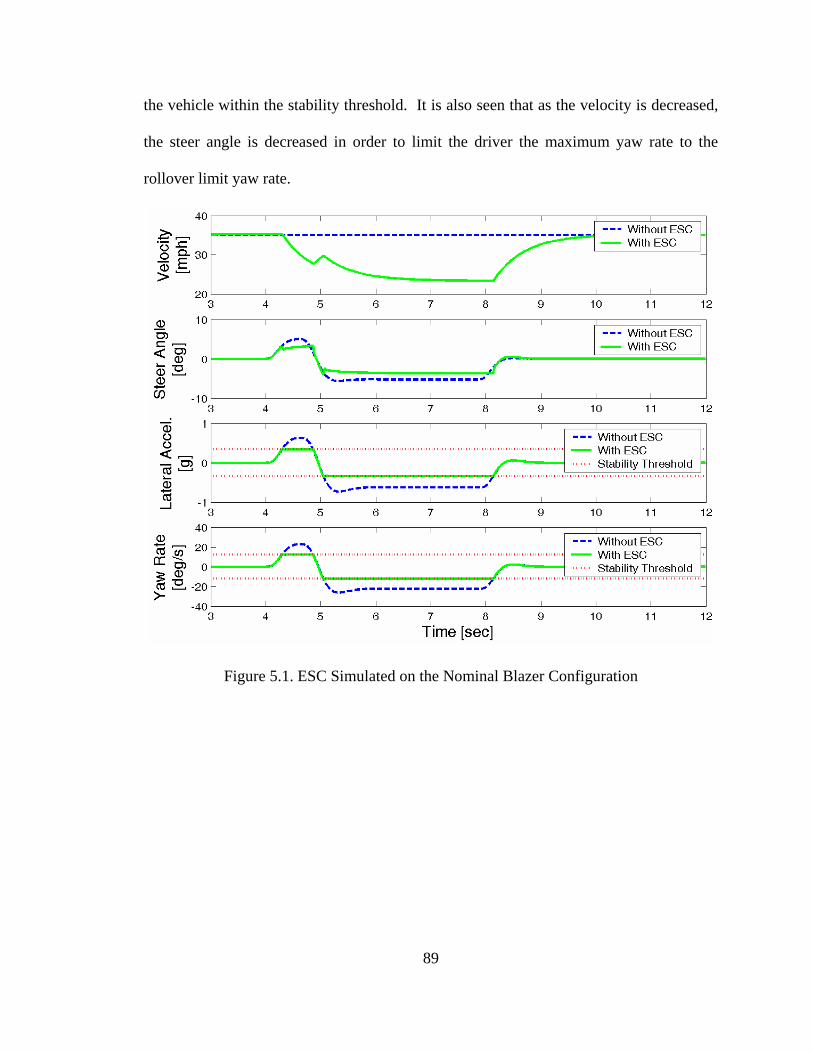
89

the vehicle within the stability threshold. It is also seen that as the velocity is decreased,

the steer angle is decreased in order to limit the driver the maximum yaw rate to the

rollover limit yaw rate.

Figure 5.1. ESC Simulated on the Nominal Blazer Configuration

90

5.3 Intelligent Vehicle Model

Although statistics were shown in Chapter 1 that ESC’s ability to prevent single

vehicle rollover is high, there is room for improvement by using an intelligent vehicle

model (IVM) that modifies the ESC’s vehicle model and controller limits. Vehicle

payload variation is the most common vehicle property varied. The ESC with the IVM is

different from a regular ESC where the vehicle model does not change, and only one

stability limit is known. The purpose of the IVM is to update the ESC controller limits as

the vehicle’s load condition changes. The IVM utilizes the stability limit for a range of

load conditions to know the vehicle’s changing rollover limit. Although not developed in

this thesis, sensors and estimation can be used to inform the IVM of weight split and CG

height changes.

Simulations were conducted to determine how the IVM could serve to increase

the effectiveness of ESC in reducing vehicle rollover. Simply adding a full load of

passengers to the Blazer can change the CG height by as much as 10%. With this

information, the Nominal Blazer was simulated driving through a Fishhook maneuver

with a maximum steer angle of 5 degrees at 24 mph. The Nominal Blazer can navigate

this maneuver without crossing the stability threshold. However, the Blazer with the

driver and four passengers has a CG height 10% higher than the Nominal configuration.

This raises the CG height from 0.663 to 0.73 meters. The Blazer with the passengers can

only negotiate the Fishhook maneuver at 22 mph. In Figure 5.2, simulation results are

seen of the Blazer with the passengers implemented with ESC. Two configurations are

91

shown, the Blazer with and without the IVM. The stability threshold for the Blazer with

the passengers is also shown.

Figure 5.2. ESC with and without IVM for CG Height Variation

The Blazer with the IVM updates the stability threshold from the Nominal

configuration of 0.33 g for lateral acceleration and 17.5 deg/s of yaw rate to the new

configuration that has the CG height 10% higher. The stability threshold for the loaded

condition is 0.295 g for lateral acceleration and 17.0 deg/s for yaw rate. It is seen in

Figure 5.2 that without the IVM, the vehicle never activates its ESC because the nominal

stability threshold is never breached. Therefore, the vehicle without IVM rolls as seen in

Figure 5.3.

92

Figure 5.3. Effect on Dynamic Behavior due to CG Height Move without IVM

However, the vehicle with IVM updates the ESC limit for yaw rate and lateral

acceleration which causes the ESC to activate. With the IVM, the vehicle never exceeds

the stability threshold and does not roll over. Table 5.1 contains the stability thresholds

for both vehicle configurations and the maximum yaw rate and lateral acceleration

achieved during the maneuver.

93

Table 5.1. ESC with and without IVM for CG Height Change

CG Height 0.663 [m] 0.73 [m] 0.73 [m]

IVM No No Yes ESC Enabled Enabled Engaged

Rollover Incident No Yes No Maneuver Maximum Lateral Acceleration

0.32g 0.32g 0.295g

Maneuver Maximum Yaw Rate

17.3 deg/sec 17.3 deg/sec 17.0 deg/sec

Stability Threshold Lateral Acceleration

0.33g 0.295g 0.295g

Stability Threshold Yaw Rate


Utilizing the IVM during CG Height changes appears to have merit, yet there is

difficulty in using the IVM during weight split variations. Table 5.2 shows the stability

threshold for the Blazer at two different weight splits, 60:40 and 40:60.

Table 5.2. Blazer Stability Threshold for Two Weight Splits

Weight Split Front:Rear Dynamic States at Rollover 60:40 40:60

Velocity [mph] 30.9 [mph] 24.4 [mph] Yaw Rate [deg/s] 19.2 [deg/s] 26.1 [deg/s]

Lateral Acceleration [g] 0.46 [g] 0.51 [g] Roll Angle [deg] 8.10 [deg] 6.84 [deg] Roll Rate [deg/s] 1.4 [deg/s] 1.5 [deg/s]

Side Slip Angle [deg] -0.05 [deg] 0.2 [deg] Side Slip Rate [deg/s] 0.5 [deg/s] 0.3 [deg/s]

Assuming that an ESC is implemented for the 60:40 weight split, it will use a

stability threshold of 19.2 deg/s for yaw rate and 0.46 g of lateral acceleration. The

maximum velocity that the 60:40 weight split can safely navigate the Fishhook maneuver

is 30.9 mph. After a change in weight split to 40:60, the maximum safe velocity that the

vehicle can achieve is lowered to 24.4 mph. However, the maximum yaw rate is

94

increased to 26.1 deg/s and the maximum lateral acceleration is increased to 0.51 g. As

was shown in Chapter 4, the vehicle’s understeer gradient decreases as the weight split is

shifted rearward. This causes the vehicle to oversteer more as the weight is shifted

rearward. For a oversteer vehicle, the maximum lateral acceleration and yaw rate

increase for the same maneuver velocity as an understeer vehicle. The use of an IVM in

this case of changing weight split is redundant. The ESC limit is set at 19.2 deg/s for yaw

rate and 0.46 g for lateral acceleration to start out with. Since a shift of the weight split

toward the rear only increases the maximum yaw rate and lateral acceleration, as shown

in Figure 5.4, the initial controller limit will suffice to keep the vehicle stable. However,

if the weight split is shifted towards the front axle of the vehicle, the rollover limit

decreases and the IVM is effective. In this case, the IVM would update the ESC’s

stability limit and cause the ESC to engage before rollover occurred. Also, note that as

the weight split deviated from the nominal configuration by being shifted to the rear, the

nominal controller limit becomes more conservative. As the controller’s limit becomes

more conservative, the vehicle’s response potential is not meet. By utilizing the IVM, the

controller limit can be updated to avoid the ESC limit from becoming ultra conservative,

and causes the vehicle’s response to be maximized. The rollover limits for the weight

split variation is shown in Figure 5.4.

95

Figure 5.4. Stability Limits for Weight Split Variation


In this chapter, a simple ESC was developed and implemented in simulation. The

vehicle’s stability threshold for changes in load conditions was used in coordination with

the ESC to increase the ESC’s ability to prevent rollover. The use of the stability

threshold to change the ESC’s limits is called an Intelligent Vehicle Model since it

updates changes to the vehicle’s parameters and stability limit. The significance of the

IVM was seen in simulation when the vehicle CG location was modified. The IVM

96

proved to be valuable for changes in CG height. However, the IVM was shown to be

redundant in cases where the vehicle’s weight split is shifted rear of the nominal

configuration, but useful in keeping the controller limit from being ultra conservative.

97

CHAPTER 6

IMPLEMENTATION ON A SCALED VEHICLE

6.1 Introduction

Rollover testing using full-size vehicles is an expensive and somewhat dangerous

endeavor. However, if dynamic behavior from the scaled vehicle tested in a controlled

environment can predict the dynamic behavior of full-size vehicles, then scaled vehicles

offer an alternative safe approach to investigate rollover. In this chapter, an analysis of

vehicle rollover is performed on a scaled vehicle. Details of the scaled vehicle and its

modifications are given, including development and implementation of a wireless IMU

for providing critical vehicle measurements. Simulation data and experimental data of

the scaled vehicle are compared to validate the dynamic similarity of the scaled vehicle

with a passenger vehicle. Stability limits for the scaled vehicle with variation of the CG

height and weight split are then derived using the vehicle simulation. Finally, a stability

control system is developed for the scaled vehicle and the stability threshold is used in

conjunction with an intelligent vehicle model to increase the stability controller’s

effectiveness.

98

6.2 Motivation for using Scaled Vehicles

Scaled vehicles have proven to be reliable test beds for a variety of applications

such as yaw controller development and tire testing [Brennan, 2000; Burns, 2002;

Hallowell, 2003]. Scaled vehicles also provide several advantages when testing and

designing. For example, costs associated with a scale model vehicle are significantly

lower and modifications are easier to make on a scale vehicle than a full-scale passenger

vehicle. Most radio control cars are purchased for less than five hundred dollars, while it

is difficult to purchase the cheapest of new passenger vehicle for fewer than ten thousand

dollars. The cost of modification and maintenance is also much less expensive on a

scaled vehicle than a passenger vehicle. The testing area required for scaled vehicles is

much smaller, allowing the testing environment to be more accurately controlled.

Compared with the Honda owned vehicle test facility in East Liberty, Ohio, where many

vehicle tests are conducted, a scaled test center is much easier to acquire and maintain.

Simple, low-cost road simulations have been built for testing scaled vehicles [Brennan

1998]. And pushing the vehicle to its limits in order to observe what happens in the non-

linear regions of the vehicle is much safer with a scale vehicle than with a full-sized

vehicle [Yih, 2000].

99

6.3 Scaled Vehicle Description

A 1:10 scale radio controlled (RC) car was used as a test bed in order to validate

the rollover experiments done in the simulation. The vehicle was modified in order to

allow the CG location, spring stiffness, and roll center height to be easily modified.

Changing the CG location provides the opportunity to view dynamics occurring at

different weight splits. It also provides a means to adjust the distance between CG height

and roll center height, which is a crucial parameter when assessing steady state roll [Hac,

2002].

There are two generations of 1/10th scale vehicles which were used to validate

simulation results. The first generation test vehicle was configured with a rear wheel

drive and front wheel steer configuration to better emulate many of today’s RWD SUVs.

Figure 6.1 shows the first generation scaled vehicle.

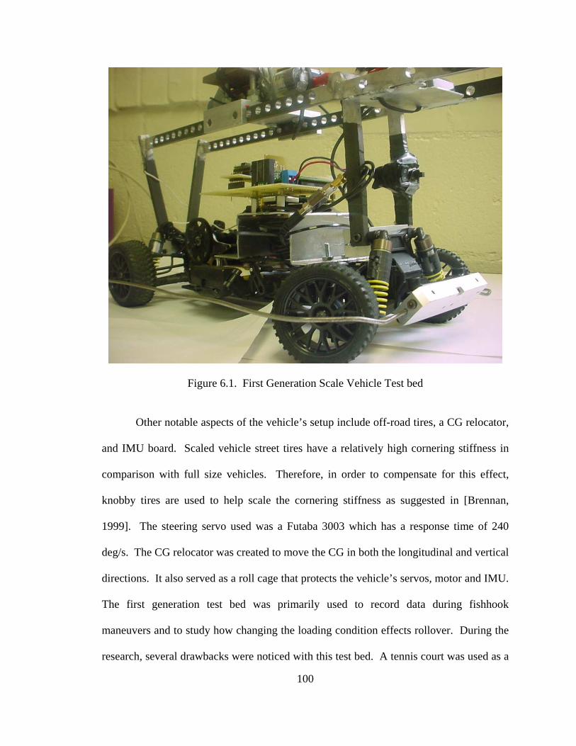
100

Figure 6.1. First Generation Scale Vehicle Test bed

Other notable aspects of the vehicle’s setup include off-road tires, a CG relocator,

and IMU board. Scaled vehicle street tires have a relatively high cornering stiffness in

comparison with full size vehicles. Therefore, in order to compensate for this effect,

knobby tires are used to help scale the cornering stiffness as suggested in [Brennan,

1999]. The steering servo used was a Futaba 3003 which has a response time of 240

deg/s. The CG relocator was created to move the CG in both the longitudinal and vertical

directions. It also served as a roll cage that protects the vehicle’s servos, motor and IMU.

The first generation test bed was primarily used to record data during fishhook

maneuvers and to study how changing the loading condition effects rollover. During the

research, several drawbacks were noticed with this test bed. A tennis court was used as a

101

test area for experiments, which provided a small area for testing. Therefore a hard

acceleration was needed in order to reach the maneuver speed, which caused major wheel

spin on the two-wheel drive vehicle and led to rapid tire wear. A lack of repeatability and

measurement of the vehicle’s true velocity were some other faults of the first generation

test bed. During testing, radio disturbances would disrupt a maneuver causing the scaled

vehicle to frequently veer off its desired course and collide with surrounding objects

during experiments, which made testing long and tedious. Additionally, the same vehicle

configuration would not consistently cause rollover at the same programmed velocity.

Other limitations included a weak roll cage, which was easily bent during rollover events,

and a CG relocator design that raised the center of gravity too high when weight split

changes were needed.

A second generation scaled vehicle was built to compete in NHTSA’s first annual

Enhanced Safety Vehicle Competition (ESV). Despite the vehicle being designed with

the intention to show a scaled safety technology for the ESV competition it also became a

vehicle dynamics and ESC test bed to study rollover. This second generation scaled

vehicle is shown in Figure 6.2.

102

Figure 6.2. Second Generation Scale Vehicle Test bed

The second generation test bed was also a 1/10th scale vehicle. However, this

vehicle was equipped with four-wheel-drive. The four-wheel-drive allowed rear wheel

spin to be eliminated during acceleration before entering a maneuver. This vehicle was

equipped with a more elaborate CG relocator, which enables the weight split to be

changed while retaining a low center of gravity. A 0.3 kg weight is positioned fore or aft

to change weight split, and risen up or down along four pieces of ¼”aluminum all-thread

to change the CG height. The weight split can also be changed by adding weights to rods

that are bolted into aluminum blocks attached fore and aft of the front and rear axles. The

roll cage is stronger than the previous generation in order to better protect the data

acquisition system. The black box in Figure 6.2 contains the wireless data acquisition

103

system which enabled improved telemetry. It was both small, and allowed wireless

feedback control to be implemented on the test bed.

The wireless feedback control system is implemented by sending driver inputs via

a steering wheel and pedal assembly. Similar to the ESC described in Chapter 5, the ESC

is preset with the yaw rate at the stability limit and decides if the driver’s inputs are

outside the vehicle’s stability region. An inertial navigation system monitors the vehicle

states and informs the ESC through a wireless connection. If the driver is within the

stability threshold, the ESC simply passes the driver’s commands to the radio transmitter.

If the driver’s inputs bring the vehicle to the stability threshold, then the controller

modifies the inputs accordingly to keep the vehicle from rolling over while maintaining

the driver’s intended path as close as possible. The inputs of the driver or the adjusted

inputs from the ESC are sent to the radio transmitter which sends commands to the

vehicle actuators. The wireless feedback control schematic is shown in Figure 6.3.

104

Figure 6.3. Vehicle Control Schematic

6.4 Data Acquisition

The first generation data acquisition system consisted of an inertial sensing

module and was constructed to meet the basic dimensional requirements of fitting on a

scaled vehicle. The system contained two gyroscopes capable of measuring 150 deg/s at

a bandwidth of 40 Hz, one two-axis accelerometer capable of measuring ±2g at 50Hz, a

GPS receiver, and a Rabbit microprocessor. The gyroscopes were oriented to obtain roll

rate and yaw rate on the scale car. The accelerometer was placed in the horizontal plane

to obtain longitudinal and lateral accelerations. The GPS unit provided vehicle position,

Wireless Communication

Driver Inputs

Vehicle Actuators

Base Station

INS

ESC Transmitter

On Board Systems

105

velocity, and course measurements, and when used in conjunction with accelerometers

and gyroscopes, can also provide measurements of vehicle sideslip [Bevly, 2001]. The

Rabbit was set up to record the inertial sensors at 100 Hz and the GPS receiver at 1 Hz

for a duration of 45 seconds at a time. After each 40 second sample period, the data must

be uploaded to a computer and the unit must be reset. This first generation data

acquisition system is shown in Figure 6.4.

Figure 6.4. First Generation IMU

The second generation data acquisition system consists of an inertial measurement

unit (IMU) that uses the same accelerometers and gyros as the first generation IMU. The

IMU board that is mounted on the second generation scaled vehicle and includes a six-

axis accelerometer/gyroscope package (3 accelerometers and 3 gyros), a GPS receiver, a

wireless transmitter, a Rabbit 2000 microprocessor, and power management components.

The wireless transmitter is a radio modem. It is used to collect inertial and position data

and send it to the base station where the ESC analyzes the vehicle’s dynamics. The

components are mounted on a printed circuit board and placed in a protective box which

is then mounted to the vehicle. The second generation data acquisition package can be

seen in Figures 6.5 and 6.6.

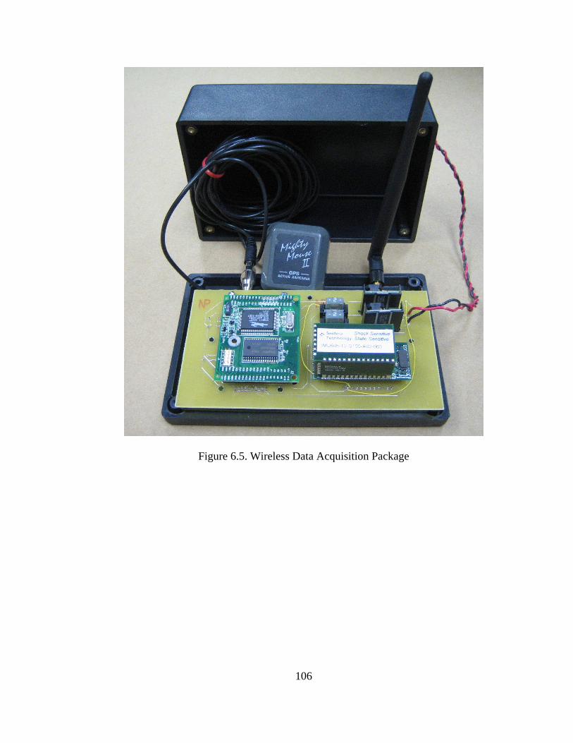
106

Figure 6.5. Wireless Data Acquisition Package

107

Figure 6.6. Second Generation Data Acquisition PCB Board. IMU and Microprocessor

shown on top, GPS Receiver and Radio Modem shown on bottom

All data sampling is controlled by the Rabbit 2000 microprocessor which uses C

code to log and transmit data. The microprocessor begins by collecting GPS and IMU

data to be sent to the base station. It then prepares a packet of data to be sent through the

wireless transmitter/receiver (MaxStream Xcite 9) which sends the data to the base

108

station. This data packet can be either literal data received from the GPS and IMU units

or raw data parsed from their messages and processed onboard. The data is received by a

wireless receiver plugged into the base station and is further processed by the ESC to

determine the vehicle’s stability. The dimensions of the INS box are 6.75” x 4.25” x

2.5”. Table 6.1 includes the specifications of the IMU.

6.5 Scaled Vehicle Simulation and Experiment Comparison

Simulations of the scaled vehicle and scaled vehicle experiments were used to

compare scaled vehicle dynamics with passenger vehicle dynamics. The simulations and

experiments were also used to verify the load dependant stability limits that were

discussed in Chapter 4.

Vehicle simulations were compared with real experimental data in order to

determine if scaled vehicle dynamics correlate with passenger vehicle dynamics. If the

vehicle model derived for the passenger vehicle (which was verified in Chapter 3) also

matches experiment data for the scaled vehicle, then scaled vehicles are valid tools for

Table 6.1 IMU Specifications

Component IMU605 - Accelerometer

IMU605 – Gyroscope

RCB-LJ– GPS

Update Rate (Hz) Up to 256 (default 60)

Up to 256 (default 60)

4

Range +/- 2g +/- 150 deg/sec n/a

Output format Digital UART Digital UART Digital UART

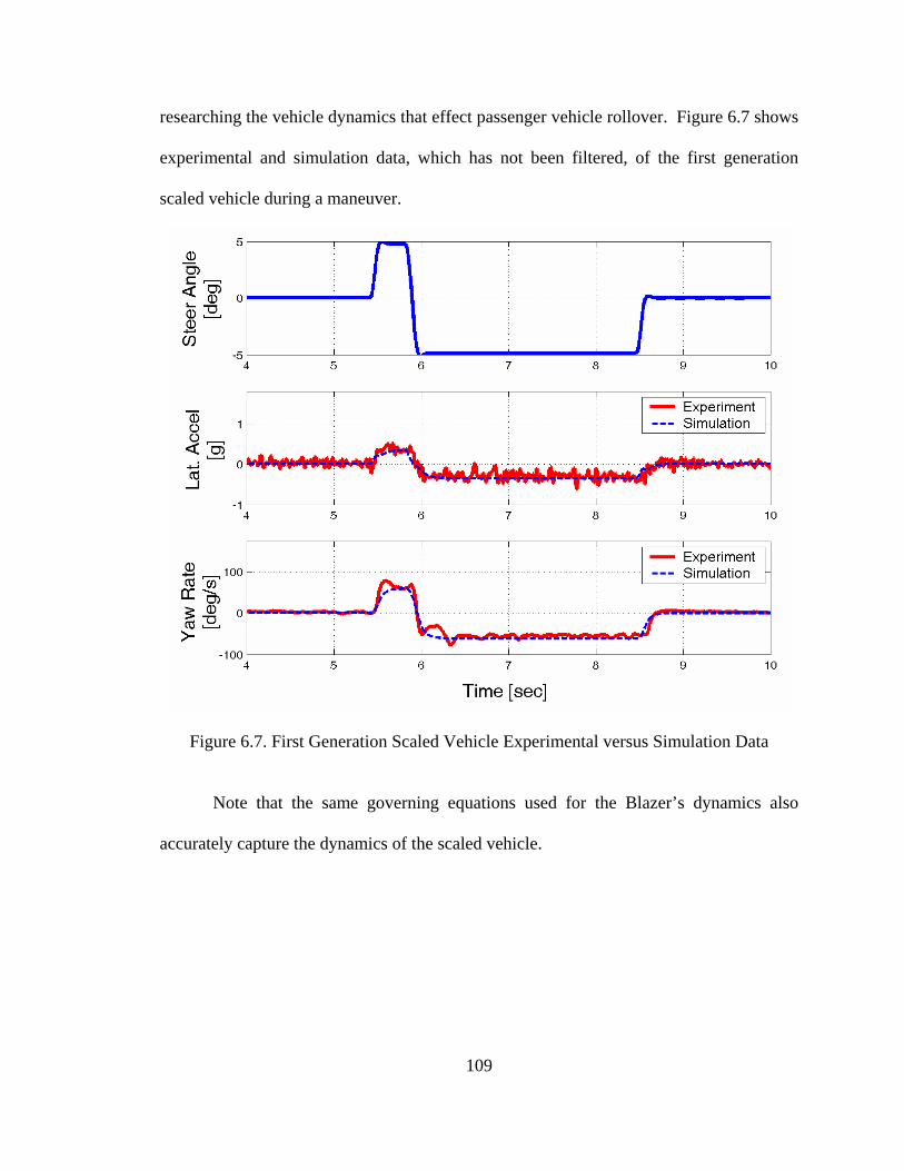
109

researching the vehicle dynamics that effect passenger vehicle rollover. Figure 6.7 shows

experimental and simulation data, which has not been filtered, of the first generation

scaled vehicle during a maneuver.

Figure 6.7. First Generation Scaled Vehicle Experimental versus Simulation Data

Note that the same governing equations used for the Blazer’s dynamics also

accurately capture the dynamics of the scaled vehicle.

110

6.6 Stability Limit Development

The stability limit developed for the Blazer in Chapter 4 was also developed for

the scaled vehicle and tested with experiments in order to assess its validity. The

simulation was limited to developing stability thresholds by changing only one vehicle

property at a time. Therefore, two separate stability thresholds were developed for the

load condition: CG height variation and weight split variation.

Vehicle simulations were used to determine the stability threshold for different

vehicle loading conditions. This was done by varying individual parameters such as the

CG height, and recording the velocity, lateral acceleration, yaw rate, and roll angle at

which rollover is detected. For these simulation experiments, a Fishhook steering profile

was chosen with a maximum steer angle of 5 degrees and a maximum steering rate of 40

degrees per second, both measured at the wheels. This profile, shown in Figure 6.8, was

filtered using a 2nd order Butterworth filter with a 1 Hz bandwidth. The velocity profile

for the maneuver was set to a constant in order to simplify the results.

111

Figure 6.8. Fishhook Steering Profile for Stability Limit Development

The second generation scaled vehicle was used to determine the stability limit

since it is the vehicle that was used in the experiments. For a given configuration, the test

maneuver was repeated with the velocity being increased by 0.1 MPH increments until

rollover occurred. NHTSA defines rollover to be the point at which both tires on one

side of the vehicle are lifted by two inches [Forkenbrock, 2003]. For this simulation

experiment, TWL over the duration of 0.4 seconds was declared to be a rollover event

since the simulation cannot determine the height of tire lift. For the simulation, TWL is

defined as the instance that wheel loads on one side of the vehicle go to zero. The

stability limit was defined as the lateral acceleration, yaw rate, and roll angle at which a

rollover event occurs. This stability limit was calculated for a variety of different vehicle

properties [Whitehead, 2004].

112

The first scaled vehicle experiment varied the CG height with a neutral

suspension setup (i.e. the weight split was set to 50:50, and the front and rear springs

were the same stiffness). Figure 6.9 shows the stability threshold for the vehicle test bed

as a function of CG height. The vehicle requires a higher lateral acceleration to rollover

as the CG height is lowered, which follows intuition and the results of the static stability

factor. The yaw rate required for rollover in this maneuver also increases as the CG

height is lowered. Once the CG height is below a certain height, the vehicle no longer

experiences rollover but begins to slide. This is due to the fact that at low CG heights, the

moment created by the un-sprung mass height and the tire lateral force does not provide

enough moment to roll the vehicle before the tires saturate. The vehicle no longer rolls

over because of a decrease in the moment in the lateral weight transfer equation caused

by the spring and damper loads, and their distance from the vehicle’s centerline, S. This

decrease in the spring and damper loads is caused by the decrease of the moment caused

by the lateral acceleration of the sprung mass and the distance between the roll center and

the CG height. The springs and dampers transfer this moment to the wheels, and since

this moment is decreased by the lowering of the CG height, the lateral weight transfer is

decreased as well.

113

Figure 6.9. Stability Limits for CG Height Variation

Note that there is a difference of 0.375 g in the lateral acceleration rollover limit.

The vehicle requires 0.472g of lateral acceleration to roll at a CG height of 0.1m, while

.097g will roll the vehicle with a CG height of 0.35m. There is also a difference of 40.3

deg/sec in the yaw rate limit for rollover. The rollover yaw rate threshold is 71.8 deg/sec

and 23.0 deg/sec for the CG heights of 0.1m and 0.35m respectively.

In order to develop the stability threshold for the longitudinal CG variation in the

simulation, the vehicle’s weight split was varied from 30:70 to 70:30, front to rear axle

weights, respectively, and the CG height was held constant at 0.15 meters. The results of

this simulation are shown in Figure 6.10.

114

Figure 6.10. Stability Limits for the Weight Split Variation

Both the yaw rate and lateral acceleration stability limits decrease as weight is

shifted from 30:70 to 36:64. The stability limits for the 30:70 weight split are 0.183 g and

44.8 deg/s. The rollover limits of the scaled vehicle for the weight split simulation vary

by 0.186 g for lateral acceleration and 15.6 deg/s for yaw rate. Stability limits are 0.309g

and 58.2 deg/s for a 70:30 weight split, and 0.166 g and 42.6 deg/s for a 36:64 weight

split. A higher lateral acceleration and yaw rate is required for vehicle rollover as the

weight is shifted towards the front axle. It is interesting to note that the vehicle

understeer gradient also increases as the weight split is shifted to the front. Therefore, a

generalization can be made that an understeer vehicle has a higher stability threshold than

an oversteer vehicle, although this trend is not always followed.

115

The change in the stability threshold during these experiments shows how

important vehicle loading data is to the ESC. For example, the stability limit changes

from 0.270 g to 0.183 g and 54.6 deg/s to 44.9 deg/s as the vehicle’s weight split is

changed 60:40 to 40:60. Therefore, if the ESC model is not updated it will use 0.270 g

and 54.6 deg/s as the stability limit, which are .087g and 9.7 deg/s more than the actual

stability limit. This may not seem like much, but the stability threshold is actually off by

32.22% for lateral acceleration and 17.77% for the yaw rate. Knowing the stability

threshold as a function of loading condition gives the ESC better ability to keep the

vehicle stable by taking out errors in the controller’s reference limits.

6.7 Stability Limit Validation

To validate the stability limits derived from the simulations, experiments which

varied the properties center of gravity height and weight split were conducted with the

scaled vehicle test bed. The first generation scale vehicle test bed operating on a concrete

tennis court was used for these experiments. This environment was preferred over a

parking lot due to the smoothness of the surface, and lack of gravel, and minimal grade.

Lack of gravel is important because gravel is perceived by the scaled vehicle test bed as a

basketball sized rock. The grade of the test environment used a constant value of 2

degrees. The size of the test area was small for high speed maneuvers, and radio

frequency disturbances frequently disrupted experiments.

116

The Fishhook maneuver used in the simulation was also used in the experimental

tests. The vehicle was driven by a computer in order to make the maneuver accurate and

repeatable. The computer was programmed to accelerate the vehicle for four seconds in

order to reach the desired velocity before the maneuver was initiated. Unlike the NHTSA

study, where the vehicle begins to coast once the maneuver is entered, the velocity for the

experiment was held constant throughout the maneuver.

Figure 6.11 shows the experiment results of the CG height variation for the

stability threshold, which follows the static stability factor and the simulation results.

The CG height was varied from 0.128 to 0.195 meters which corresponds a SSF variation

of 0.4564 to 0.6138. The results of the experiment closely match the simulation. For a

center of gravity height of 0.16 meters, the simulation shows the vehicle rolling over at a

velocity of 6.25 MPH while the rollover velocity of the experiment was recorded at

approximately 6.5 MPH. The proximity of these results provides validity gives value to

the developed stability limits. Additionally, it is important to note that the same trend is

evident in both experiment and simulation.

117

5.5

6

6.5

7

7.5

8

8.5

9

9.5

0.12 0.14 0.16 0.18 0.2

CG Height (m)

Rol

love

r V

eloc

ity (

MP

H)

Figure 6.11. Experimental Stability Limit for Variations in the CG Height

The second set of experiments varied the longitudinal weight distribution. The

first generation test bed was again used at the tennis court to perform this test. The

maneuver and computer controls were kept the same as in the previous CG height

variation experiments.

Figure 6.12 shows the experimental stability limit for rollover. It can be seen that

the experimental results validate the simulation shown previously in Figure 6.10.

Although weight split variation in the simulation and experiment follow the same derived

trend, their rollover velocities do not match. This is due to the center of gravity height

being higher in the simulation than the experiment. With the CG height setup in the

experiment, the vehicle will not roll at weight splits favored to the front because of tire

saturation. Qualitatively, the experimental results do follow the simulation trend which

acknowledges that the vehicle is less prone to rollover as the weight split is shifted

towards the front of the vehicle.

118

99.5

1010.5

1111.5

12

12.513

13.514

40 50 60 70 80 90

Percent Total Weight on Rear Axle

Ro

llove

r Ve

loci

ty (

MP

H)

Figure 6.12. Weight Split Variation Experiment Stability Limit

6.8 Electronic Stability Control

As described in Chapter 5, the ESC is implemented as a PI controller via

MATLAB simulation. The ESC’s purpose is to keep the vehicle within the stability

threshold. The stability limit is defined as the lateral acceleration and yaw rate at which

the vehicle will experience TWL during a fishhook maneuver. The ESC monitors these

two states and when the stability threshold is approached, the controller adjusts steer

angle and velocity to maintain stability. When the ESC enabled vehicle is below the

119

stability limits, the ESC does not modify with the driver’s inputs. However, once the

driver’s inputs exceed the stability limit, the ESC adjusts the steer angle and velocity to

limit the yaw rate to the yaw rate stability limit and limit the lateral acceleration to the

lateral acceleration stability limit. Since the scaled vehicle used was an off-the-shelf

radio control vehicle, the only actuators available to the ESC on the scaled vehicle

testbed were the steering servo and velocity control unit which brakes and accelerates the

rear wheels. Figure 6.13 shows a simulated scaled vehicle with and without the ESC

enabled. The maneuver that the vehicle is attempting to negotiate is a Fishhook

maneuver at a maximum steer angle of 5 degrees with a maximum steer rate of 40

degrees per second at the tires. The driver’s desired velocity is 8 MPH.

Figure 6.13. Results for the Fishhook Maneuver with and without ESC enabled

120

In order to maintain stability in this maneuver, the ESC adjusts the steering angle

and actuates the brakes in order to not exceed the lateral acceleration and yaw rate limit.

However, the ESC still tries to follow the driver’s desired path by calculating the desired

radius of the turn. The lateral acceleration stability threshold for this particular vehicle

setup is 0.25g and the yaw rate stability threshold is 53.6 deg/sec. Figure 6.13 reveals

how the ESC keeps the vehicle within the stability threshold when it would otherwise

become unstable.

6.9 Intelligent Vehicle Model (IVM)

As a vehicle’s payload changes, the Intelligent Vehicle Model (IVM) gives the

controller knowledge of the change in the stability limit and adjusts the controller limits

accordingly. Sensors, in conjunction with vehicle parameter estimation techniques would

constantly monitor the vehicle weight split and CG height. The stability limit for the load

condition would then be used as the controller’s limit in the ESC.

In order to see how the IVM can improve the ESC effectiveness, a simulation was

performed with the scaled vehicle model using a 60:40 and 40:60 weight split (front to

rear axle weights, respectively). The CG height and static stability factor were held

constant for this property variation. Again, a Fishhook maneuver with a maximum steer

angle of 5 deg and maximum steer rate of 40 deg/s was used for the simulation. The

121

vehicle longitudinal velocity was set to 6 MPH and held constant throughout the

maneuver.

In the initial configuration, the scaled vehicle had a weight split of 60:40 front to

rear. The stability limit for this load condition is 0.270 g for lateral acceleration and 53.6

deg/sec for yaw rate. The ESC vehicle model is initially programmed to use these state

limits in order to maintain stability. Since the vehicle does not exceed this limit during

the maneuver, the ESC is never activated. It can be seen from the wheel loads in Figure

6.14 that the vehicle does not roll, but one wheel lift does occur.

Figure 6.14. Results for the Fishhook 1a with 60:40 Weight Split

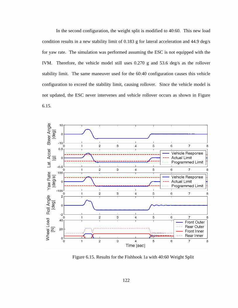
122

In the second configuration, the weight split is modified to 40:60. This new load

condition results in a new stability limit of 0.183 g for lateral acceleration and 44.9 deg/s

for yaw rate. The simulation was performed assuming the ESC is not equipped with the

IVM. Therefore, the vehicle model still uses 0.270 g and 53.6 deg/s as the rollover

stability limit. The same maneuver used for the 60:40 configuration causes this vehicle

configuration to exceed the stability limit, causing rollover. Since the vehicle model is

not updated, the ESC never intervenes and vehicle rollover occurs as shown in Figure

6.15.

Figure 6.15. Results for the Fishhook 1a with 40:60 Weight Split

123

However, if the vehicle was equipped with the IVM along with the ESC, then the

ESC would have known the correct stability limits. Therefore, the ESC could use the

updated stability limit for the modified weight split. This would have enabled the ESC to

correctly prevent the rollover as shown in Figure 6.13. A comparative analysis of these

configurations is given in Table 6.2.

Table 6.2. ESC with and without IVM

Weight Split Front:Rear 60:40 40:60 40:60

IVM No No Yes ESC Engaged Disengaged Engaged

Rollover Incident No Yes No Maneuver Maximum Lateral Acceleration

0.25g 0.25g 0.18g

Maneuver Maximum Yaw Rate


Stability Threshold Lateral Acceleration

0.270g 0.183g 0.183g

Stability Threshold Yaw Rate



In this chapter, scaled vehicles have been shown to be valuable in evaluating

vehicle loading conditions and their correlation with rollover. It has also been shown that

scaled vehicles are valuable tools for studying ESC systems. Section 6.6 quantified a

stability threshold in simulation for a scaled vehicle, and proposed the use of an IVM

system. The IVM updates the stability threshold in the vehicle model for an ESC system

124

as the vehicle’s payload changes. Section 6.7 verified the stability threshold with scaled

vehicle experiments. Section 6.9 provided a scenario in which implementing an IVM

would prevent rollover, while an ESC without IVM would not. Furthermore, this chapter

has shown that scaled vehicles can be used to validate simulation results as well as

provide valid information on the behavior of full scale passenger vehicles.

125

CHAPTER 7

CONCLUSION

7.1 Summary

An investigation of rollover propensity using simulation and experimental data

has been presented. A vehicle model was developed and validated for studying rollover

propensity. This vehicle model was then use to explore the changes that vehicle

parameters have on rollover propensity. Stability thresholds for a range of vehicle load

conditions were developed as well. An ESC was developed for mitigating rollover in

simulation. Also, an IVM was developed and implemented with the ESC in order to

improve ESC’s effectiveness in preventing rollover. Finally, a scaled vehicle was used to

validate the research. A summary of the research highlights in each chapter is provided

below followed by a discussion of recommendations for future research.

In Chapter 2, a vehicle model was created to capture the major dynamics that

govern vehicle rollover. Both non-linear yaw and roll dynamics were used to reproduce

the transient dynamics in these axes. Newton’s method, using FBDs, were used to

develop the governing equations of motion. The non-linear, Pacejka, ‘Magic Formula’

tire model was used to model the tires. The diagrams and equations were detailed in the

order in which they were used to develop the vehicle model.

126

Chapter 3 contains the evaluation and validation of the vehicle model developed

in Chapter 2. In Section 2.2, the steady state results of the steady state roll equations

were compared with those of the transient roll equations. The transient roll equations

yielded the same steady state dynamic state values as the steady state roll equations. This

validated the steady state dynamic states of the transient roll equations used in the vehicle

model. Section 2.3 contained NHTSA Phase IV data which validated the transient

dynamics of the yaw and roll equations in the vehicle model by matching with the

simulation data. Experimental results using a transient maneuver with a Blazer at Auburn

University provided further validation of the transient vehicle model. Finally, a

discussion on the effect of roll centers below the un-sprung mass on weight transfer was

given.

In Chapter 4, the correlation between vehicle load condition and rollover

propensity was investigated. Analysis of the various load configurations of the NHTSA

Blazer led to the development of a vehicle rollover stability threshold. The rollover

stability threshold was derived as a function of various vehicle dynamic states such as

lateral acceleration, yaw rate, and roll rate.

A simple ESC was developed in Chapter 5, and it is simulated on a Blazer. An

IVM was developed to aid the ESC in preventing rollover. It utilized the stability

threshold created in Chapter 4 with knowledge of vehicle properties changes to update

the controller’s vehicle model and state limits. It was shown that the IVM could improve

ESC effectiveness during CG height changes. However, the IVM proved to be redundant

as the vehicle’s weight split was shifted to the rear axle.

127

In Chapter 6, the experimental test bed developed in this study allowed the

robustness of ESC to be evaluated via changing vehicle properties such as weight split,

center of gravity height, and suspension setup. These scenarios simulate changes in

vehicle loading and suspension modifications, which are relevant in today’s world of

transporting children to soccer practice in SUVs, low rider hot rods, and modified four

wheel drive vehicles. The scaled vehicle was used as a test bed to validate the stability

limits created in simulation, explore vehicle properties that influence rollover, and

investigate ESC algorithms. It is equipped with telemetry which consists of GPs and INS

sensors. This chapter also quantified a rollover stability limit for the scaled vehicle and

utilized the IVM, which updates the stability threshold in the vehicle model of an ESC.

This chapter developed a scenario demonstrating that the IVM would aid in preventing

rollover. The significance of the Intelligent Vehicle Model can be seen from the

exercises in Section 6.9. IVM is a tool that ESC can use to improve its ability to prevent

vehicle rollover.

7.2 Recommendations for Future Work

Results form this thesis should extended to derive the stability limit as a function

of more vehicle properties. The vehicle properties that should be studied next include

front and rear roll center heights as well as front and rear roll stiffness and damping. The

128

vehicle states that should be monitored in the stability threshold include yaw rate, lateral

acceleration, roll angle, roll angle rate, side slip rate, and side slip angle.

The effect of tire properties should be further investigated for a wider range of

paths and maneuvers, not just for steering profiles. This will provide a more accurate

analysis of how a tire’s cornering stiffness and peak lateral force effect vehicle rollover.

A higher DOF model, such as Adams or CARSIM, could also be used to derive

the stability limits. The higher DOF models will include the suspension kinematics and

dynamics of the un-sprung mass. These results should be compared with the results of

the work presented in this thesis.

Since the ESC and IVM were only tested in simulation, further research could be

conducted via experiments. Experimental data verifying the effectiveness that IVM has

on preventing rollover is worth acquiring. Either a passenger vehicle or scaled vehicle

could be used. Though the research presented in this thesis used the Fishhook maneuver,

other maneuvers such as the ISO-3888 lane change maneuvers could be used. This

maneuver requires a driver to follow a marked path instead of a steer profile. This would

provide further validation of the ESC and IVM developed in this thesis.

Methods to inform the IVM of vehicle property changes should be explored.

String potentiometers can be tuned to measure normal wheel loads. Accelerometers from

an on-board IMU could be used with the wheel loads to determine the vehicle’s weight

split in a static case. Methods such as using a Kalman Filter to estimate the weight split

should also be developed. A method to accurately estimate the CG height should also be

derived and implemented. These methods to determine the vehicle load condition status

could be implemented in simulation and experiments.

129

The scaled vehicle research in this thesis provided a relatively inexpensive means

of acquiring real vehicle data. While this test bed provided experimental data, it could be

improved. Because of the size of the 1:10th scale vehicle issues such as implementing

sensors and finding a suitable test environment were never fully solved. For instance, a

pebble to a full size vehicle is magnified 10 times for the 1:10th scale vehicle, and a

seemingly smooth surface for a passenger vehicle is rough to a scaled vehicle. For future

work, a larger scale vehicle (1:4th) should be used than the one used in this study. A

larger vehicle, though more expensive, would be easier to instrument and might

ultimately produce more accurate results.

130

REFERENCES [1] Allen, R. W., Szostak,H.T, Rosenthal, T. J. and Klyde,D. H. 1990. “Field

Testing and Computer Simulation Analysis of Ground Vehicle Dynamic Stability.” SAE Paper No. 900127.

[2] Amberkar, S., et. al., “A Control System Methodology for Steer by Wire Systems.” 2004. SAE Paper No. 2004-01-1106.

[3] Baumann, F.W., et. al., “Effects Causing Untripped Rollover of Light Passenger Vehicles in Evasive Maneuvers.” 2004. SAE Paper No. 2004-01-1057.

[4] Bevly, D. M., Ryu, J., Sheridan, R., Gerdes, J. C, "Integrating INS Sensors with GPS Velocity Measurements for Continuous Estimation of Vehicle Side-Slip and Tire Cornering Stiffness," Proceedings of the 2001 American Control Conference, Vol.1, June 2001, pp.25-30.

[5] Brennan, S., et. al., “The Illinois Roadway Simulator – A Hardware-in-the-Loop Testbed Vehicle Dynamics and Control.” Proceedings of the American Control Conference. June, 1998.

[6] Brennan, S. and Alleyne, A. “Using Scale Testbed: Controller Design and Evaluation.” IEEE Control Systems Magazine, vol 21, 2001, pp. 15-26.

[7] Brennan, S. and Alleye, A. “Modeling and Control Issues Associated With Scaled Vehicles,” 1999, University of Illinois at Urbana-Champaign.

[8] Brennan, S. and Alleyne, “The Illinois Roadway Simulator: A Mechatronic Testbed for Vehicle Dynamics and Control.” IEEE Transactions on Mechatronics. Vol. 5, No. 4, pp. 349-359, December 2000.

[9] Brennan, S., “Similarity Conditions for Comparing Closed-Loop Vehicle Roll and Pitch Dynamics.” Proceeding of the 2004 American Control Conference. Boston, MA. June 30 – July 2, 2004.

[10] Broulhiet, G., “The Suspension of the Automobile Steering Mechanism: Shimmy and Tramp”, Bull Soc. Ing. Civ. Fr. 78, pp. 540-554, July 1925.

[11] Burns, Stephen R., O’Brien, Richard T., Piepmeier, Jenelle A., “Steering Controller Design Using Scale-Model Vehicles,” 2002, IEEE Paper No. 0-7803-7339-1/02

[12] Carlson, C. R., and Gerdes, J. C., “Optimal Rollover Prevention with Steer by Wire and Differential.” Proceedings of IMECE 2003.

[13] Christos, J. P. and Guenther, D. A. “The Measurement of Static Rollover Metrics,” 1992, SAE Paper No. 920582

[14] Cooperrider, N. K., Hammound, S. A. and Thomas, T.M. “Testing and Analysis of Vehicle Rollover Behavior,” 2000, SAE Paper No. 900366

[15] Day, T. D., and Garvey, J. T., “Applications and Limitations of 3-Dimensional Vehicle Rollover Simulation.” 2000. SAE Paper No. 2000-01-0852.

[16] D’Entremont, K. L., Zhengyu, L. and Nalecz, A. G. “An Investigation into

131

Dynamic Measures of Vehicle Rollover Propensity,” 1993, SAE Paper No. 930831

[17] Dixson, J. C., “Tires, Suspension and Handeling” Society of Automotive Engineers. Warrendale, PA. ISBN: 1-56091-831-4.

[18] Dugoff, H., Fancher, P.S., Segel, L., “Tire Performance Characteristics Affecting Vehicle Response to Steering and Braking Control Inputs.” Report for Tire System Section, Office of Vehicle Systems Research. National Bureau of Standards, Washington, D.C. August, 1969

[19] Dugoff, H., Fancher, P.S., Segel, L., “An Analysis of Tire Traction Properties and their influence on Vehicle Dynamic Performance.” SAE Paper 700377, 1970

[20] Eger, R., et. al., “Rollover Simulation Based on a Nonlinear Model.” 1998. SAE Paper No. 980208.

[21] Ellis, J. R., “The Dynamics of Vehicles During Braking.” Symposium on the Control of Vehicles, Institution of Mechanical Engineers, June 1963

[22] Fatality Analysis Reporting System (FARS) Web-Based Encyclopedia. National Center for Statistics and Analysis, National Highway Traffic Safety Administration, U.S. Department of Transportation. http://www-fars.nhtsa.dot.gov/.

[23] Forkenbrock, G.J., Garrott, W.R., Heitz, M. and O’Hara, B.C. NHTSA. 2002. “A Comprehensive Experimental Examination of Test Maneuvers that May Induce On-Road, Untripped, Light Vehicle Rollover – Phase IV of NHTSA’s Light Vehicle Rollover Research Program” (October). Report No. DOT HS 809 513.

[24] Forkenbrock, G. J., Garrott, W.R., Heitz M. and O’Hara, B.C. 2003. “An Experimental Examination of J-Turn and Fishhook Maneuvers that May Induce On-Road, Untripped, Light Vehicle Rollover.” SAE Paper No. 2003-01-1008.

[25] Fromm, H., “Brief Report on the History of the Theory of Shimmy”, NACA TM 1395, pp. 181, 1954.

[26] Garrott, W. R., and Heydinger, G. J. 1992. An Investigation, Via Simulation, of Vehicle Characteristics that Contribute to Steering Maneuver Induced Rollover. SAE Paper No. 920585.

[27] Gillespie, T. D. 1992. “Fundamentals of Vehicle Dynamics.” Society of Automotive Engineers. Warrendale, PA. ISBN: 1-56091-199-9.

[28] Ginsberg, J. H., “Advance Engineering Dynamics.” 2nd ed. Cambridge University Press, 1998. ISBN: 0-521-47021-8.

[29] Hac, A. 2002. Rollover Stability Index Including Effects of Suspension Design. SAE Paper No. 2002-01-0965.

[30] Hac, A., et. al., “Detection of Vehicle Rollover.” 2004. SAE Paper No. 2004-01-1757.

[31] Hallowell, Stephen J. and Ray, Laura R. “All Wheel Driving Using Independent Torque Control of Each Wheel, 2003,” IEEE Paper No. 0-7803-7896-2/03

[32] Hilton, J., and Shankar, U., “Motor Vehicle Traffic Injury and Fatality Estimates – 2002 Early Assessment,” Report No. DOT HS 809 586, May 2003, p. 15

[33] Huang, J., et. al., “Control Oriented Modeling for Enhanced Yaw Stability and

132

Vehicle Steerability.” Proceeding of the 2004 American Control Conference. Boston, MA. June 30 – July 2, 2004.

[34] Johansson, B., and Gafvert, M., “Untripped SUV Rollover Detection and Prevention.” 43rd IEEE Conference on Decision and Control. December 14 – 17, 2004.

[35] Klein, T. M., “A Statistical Analysis of Vehicle Rollover Propensity and Vehicle Stability.” 1992. SAE Paper No. 920584.

[36] Milliken, D. L. and Milliken, W. F. 1995. Race Car Vehicle Dynamics. Society of Automotive Engineers. Warrendale, PA. ISBN: 1-56091-526-9.

[37] Morrison, W. R. B., “On the Lateral Dynamics of an Automobile in Accelerated Motions.” Mechanical and Chemical Engineering Transactions, The Institution of Engineers, Australia, November 1967

[38] Newton, I., “Philosophiæ Naturalis Principia Mathematica.” Londini : Jussu Societatis Regiae ac Typis Josephi Streater. Prostat apud plures bibliopolas, 1687.

[39] NHTSA. Phase IV Rollover Testing. 2002. George Washington Transportation Research Institute.

[40] NHTSA 2005: SafeCar.gov, Rollover. 18, Oct. 2005,

< http://www.nhtsa.dot.gov/cars/testing/ncap/Rollover/Index.htm>.

[41] Nishio, A., et. al., “Development of Vehicle Stability Control System Based on Vehicle Sideslip Angle Estimation.” 2001. SAE Paper No. 2001-01-0137.

[42] Pacejka, H. B., Bakker, E., and Nyborg, L., “Tyre Modelling for Use in Vehicle Dynamics Studies.” SAE Paper No. 870421, 1987

[43] Pacejka, H. B., Bakker, E., and Lidner L., “A New Tire Model with an Application in Vehicle Dynamics Studies.” SAE Paper No. 890087, 1989.

[44] Plumlee, J. H., et. al. “Control of a Ground Vehicle Using Quadratic Programming Based Control Allocation Techniques.” 2004.

[45] Ponticel, P. 2003. “Dynamic Testing Rollover on the Way,” Automotive Engineering International (November 2003): 26-28.

[46] Radt, H. S., and Milliken, W. F., “Motions of Skidding Automobiles.” Paper 205-A, Presented at SAE Summer Meeting, Chicago, June 1960

[47] Radt, H. S. and Pacejka, H. B., “Analysis of the Steady-State Turning of an Automobile.” Symposium on the Control of Vehicles, Institution of Mechanical Engineers, June 1963

[48] Ryu, J., et. al., “Vehicle Sideslip and Roll Parameter Estimation using GPS.” Design Division Stanford University.

[49] Schubert, P. J., et. al. “Electronic and Algorithms for Rollover Sensing.” 2004. SAE Paper No. 2004-01-0343.

[50] Travis, W., Whitehead, R., Bevly, D. M., and Flowers G. T. “Using Scaled Vehicles to Investigate the Influence of Various Properties on Rollover Propensity.” Proceedings of the 2004 American Controls Conference, Boston, 30 June – 2 July, 2004.

[51] Tseng, H. E., et.al., “Technical Challenges in the Development of Vehicle Stability Control System.” Proceedings of the 1999 IEEE International Conference on Control Applications. August 22-27, 1999.

133

[52] U.S. Department of Transportation, National Highway Traffic Safety Administration, The Economic Impact of Motor Vehicle Crashes 2000 (Washington, DC: 2002), also available at http://www.nhtsa.dot.gov/people/economic, as of December 2002.

[53] van Zanten, A.T., “Bosch ESP Systems: 5 Years of Experience.” 2000. SAE Paper No. 2000-01-1633.

[54] Viano, D. C. and Chantal, P. “Case Study of Vehicle Maneuvers Leading To Rollovers: Need for a Vehicle Test Simulating Off-Road Excursions, Recovery and Handling,” 2003 SAE Paper No. 2003-01-0169.

[55] Vilaplana, M.A., et. al., “Control of Sideslip and Yaw Rate in Cars Equipped with 4-Wheel Steer-by-Wire.” 2004. SAE Paper No. 2004-01-2076.

[56] Voelcker, John. “Top Ten Tech Cars: A Year of Stability.” IEEE Spectrum. March 2005: 22-30.

[57] Whitehead, R., Travis, W., Bevly, D. M., Flowers, G. T., “A Study of the Effect of Various Vehicle Properties on Rollover Propensity,” 2004, SAE Paper No. 2004-01-2094.

[58] Wilde, J. R., et. al. “Experimental Evaluation of Fishhook Maneuver Performance of a Kinetic Suspension System.” 2005. SAE Paper No. 2005-01-0392.

[59] Yih, Paul. “Radio Controlled Car Model as a Vehicle Dynamics Test Bed,” Mechanical Engineering Department, Stanford University, Sept. 2000

134

APPENDICES

135

APPENDIX A

VEHICLE PROPERTIES

A.1 Introduction

Appendix A.2 contains a list and description of the vehicle properties used in the

vehicle model developed in Chapter 2. Appendix A.3 contains the values of the vehicle

properties for each of the Blazer configurations used in the NHTSA Phase IV

experiments.

136

A.2 Garage Legend

Name Description Units MT Vehicle Total Mass kg M Vehicle Sprung Mass kg m Vehicle Un-Sprung Mass kg g Gravitational Constant m/s2

Wt Total Vehicle Weight N Iz Vehicle Yaw Inertia N-m-s2 Ix Vehicle Roll Inertia N-m-s2

WB Vehicle Wheelbase m a Distance from the CG to the front axle m b Distance from the CG to the rear axle m

hcgM CG height of Sprung Mass m hcgm CG height of Un-Sprung Mass m hrcf Front Roll Center height m hrcr Rear Roll Center height m trkf Front vehicle track m trkr Rear vehicle track M Skf Distance between front springs M Skr Distance between rear springs M Sbf Distance between front dampers M Sbr Distance between rear dampers M

Karbf Front Stabilizer, (anti-roll bar) Stiffness N-m/rad Karbr Rear Stabilizer, (anti-roll bar) Stiffness N-m/rad Ksf Front Spring Stiffness N/m Ksr Rear Spring Stiffness N/m Bf Front Shock Damping Coefficient N-s/m Br Rear Shock Damping Coefficient N-s/m

137

A.3 Garage Vehicles and Parameters

Parameter Vehicle Description Nominal Blazer RRR Blazer RMB Blazer

MT 1907 kg 1988.78 kg 2237.71 kg M 1525 kg 1606.78 kg 1855.71 kg m 382 kg 382 kg 382 kg g 9.81 m/s2 9.81 m/s2 9.81 m/s2

Wt 18707.67 N 19509.93 N 21951.94 N Iz 3833.31 N*m*s2 4094.98 N*m*s2 N*m*s2 Ix 734.04 N*m*s2 813.49 N*m*s2 N*m*s2

WB 2.718 m 2.718 m 2.718 m a 1.216 m 1.216 m 1.522 m b 1.502 m 1.502 m 1.196 m

hcgM 0.6629 m 0.6960 m 0.6614 m hcgm 0.35 m 0.35 m 0.35 m hrcf -0.1 m -0.1 m -0.1 m hrcr 0.35 m 0.35 m 0.35 m trkf 1.445 m 1.445 m 1.445 m trkr 1.405 m 1.405 m 1.405 m Skf 0.7747 m 0.7747 m 0.7747 m Skr 0.9906 m 0.9906 m 0.9906 m Sbf 0.7747 m 0.7747 m 0.7747 m Sbr 0.7620 m 0.7620 m 0.7620 m

Karbf 700 N/deg 700 N/deg 700 N/deg Karbr 400 N/deg 400 N/deg 400 N/deg Ksf 75000 N/m 75000 N/m 75000 N/m Ksr 70000 N/m 70000 N/m 70000 N/m Bf 5000 N*s/m 5000 N*s/m 5000 N*s/m Br 4000 N*s/m 4000 N*s/m 4000 N*s/m

138

APPENDIX B

SCALED VEHICLE PROPERTIES

B.1 Introduction

Appendix B contains the parameters of the scaled vehicle. These parameters are

used in the vehicle simulation and come from the scaled vehicle that was used in the

experiments.

139

B.2 Scaled Vehicle Parameters

Parameter Description Value Units MT Vehicle Total Mass 3.20 kg M Vehicle Sprung Mass 2. kg m Vehicle Un-Sprung Mass 0.276 kg g Gravitational Constant 9.81 m/s2

Wt Total Vehicle Weight 31.392 N Iz Vehicle Yaw Inertia 0.20 N-m-s2 Ix Vehicle Roll Inertia 0.10 N-m-s2

WB Vehicle Wheelbase 0.2556 m a Distance from the CG to the front axle 0.1374 m b Distance from the CG to the rear axle 0.1182 m

hcgM CG height of Sprung Mass 0.1565 m hcgm CG height of Un-Sprung Mass 0.020 m hrcf Front Roll Center height 0.010 m hrcr Rear Roll Center height 0.0127 m trkf Front vehicle track 0.1683 m trkr Rear vehicle track 0.1746 M Skf Distance between front springs 0.0492 M Skr Distance between rear springs 0.0762 M Sbf Distance between front dampers 0.0492 M Sbr Distance between rear dampers 0.0762 M Ksf Front Spring Stiffness 300 kN/m Ksr Rear Spring Stiffness 300 kN/m Bf Front Shock Damping Coefficient 100 N-s/m Br Rear Shock Damping Coefficient 100 N-s/m

140

APPENDIX C

VEHICLE SIMULATION

C.1 Introduction

There are 15 MATLAB functions and scripts that make up the vehicle simulation.

As stated in Chapter 2, the vehicle simulation is 3 DOF including the yaw and roll

transient dynamics. The trapezoidal method is used to solve the integrals. The time step

must be set at .001 seconds to achieve good results when using this method. The various

pieces of MATLAB code are shown in the following sections of Appendix C.

C.2 Vehicle Simulation Layout

The simulation beings with the function ‘main.m.’ The vehicle, maneuver, and

velocity profile are each chosen by the user in this function. The property variation can

also be chosen from the ‘main’ function. The ‘Garage.m’ contains vehicle properties for

various vehicles. The steering profile is produced in the ‘steer_profile.m’ function.

‘Velocity.m’ produces the longitudinal velocity profile for the maneuver. The

‘property_changer.m’ allows vehicle properties to be varied until two-wheel-lift is

detected in the ‘two_wheel_lift_detector’ script. The simulation switch script contains

141

the numerical integration to solve the equations of motion and yield the vehicle’s

dynamic states. ‘RubberandString.m’ is called from the simulation switch when a value

for tire lateral force is required. Various tire models are found in this function such as the

non-linear, Pacejka ‘Magic Formula,’ and the linear tire model.

C.3 Main.m

% Vehicle Simulation close all clear all clc % Property you wish to vary % 0 - No Changes % 100 - Nominal Vehicle Condition looking for wheel lift % 1 - Weight Split % 2 - CG Height prop=1; % Simulation type % '100' - Steady State Roll % '300' - Transient Roll sim=300; % Vehicle Model car='2001 Blazer Nom'; % Maneuver Profile % step - Step Steer % 1a - Fishhook maneuver='1a'; % Max steer angle [deg] A=5; max_steer=A; % Velocity Profile % step - Step Profile % ramp a - Contant ramp

142

% ramp - Ramp at a given acceleration % coast - Coast Down vel_profile='step'; if prop == 0 | 100 ZZ=0; speed_i=15; % [MPH] Velocity of No Change Option 0 else ZZ=1; speed_i=15; % [MPH] Initial Velocity of Property Changer Option 1:10 end % Wheel Lift Detector % 1 1-Wheel-Lift % 2 2-Wheel-Lift wheel_lift_detector=2; lift_time=1; %ts*sec - value being the duratin of wheel lift ie. value at 1000 = 1 sec wheel lift % Tire Model % Linear % Pacejka % Dugoff tire='Pacejka'; % Simulation Time endtime=8; % 8 seconds is minimum time for steer profile 1a ts=0.001; % Sample Time NN=endtime/ts; % # of calculations % Loading Vehicle Data [MT,M,m,g,Wt,Iz,Ix,zeta,a,b,h_cg_M,h_cg_m,h_rc_f,h_rc_r,trk_f,trk_r,... Sk_f,Sk_r,Sb_f,Sb_r,Sarb_f,Sarb_r,ks_f,ks_r,... karb_f,karb_r,Ca_f,Ca_r,SIS_const,steer_ratio,WB,b_f,... b_r] = garage(car); disp('Vehicle Parameters Loaded...') % Loading Steering Profile del=steer_profile(maneuver,max_steer,SIS_const,endtime,ts,steer_ratio); disp('Steering Profile Loaded...') % Roll Stiffness kphi_f = karb_f+0.5*ks_f*Sk_f^2; % Front Roll Stiffness [N*m*rad] kphi_r = karb_r+0.5*ks_r*Sk_r^2; % Rear Roll Stiffness [N*m*rad] kphi_t = kphi_f+kphi_r; % Total Roll Stiffness % Calculating the roll center at the CG

143

[h_rc_cg]=roll_center_height(WB,a,h_rc_f,h_rc_r); % Property Changer Property_Changer % Initial Conditions initial_variables % Property Variation Loop for qq = 1:QQ flag=0; two_wheel_lift_i(1:NN)=0; two_wheel_lift_o(1:NN)=0; t_w_l_i(1:NN)=0; t_w_l_o(1:NN)=0; w_l_fi(1:NN)=0; w_l_fo(1:NN)=0; w_l_ri(1:NN)=0; w_l_ro(1:NN)=0; zz=0; while zz <= ZZ while flag == 0 % Velocity speed=speed_i+(zz/10); %(zz increments 1 each step, adjust the denominator for mesh density) % Ramp Acceleration Note: Must be an even number accel=2; % Loading Velocity Profile vel=velocity(vel_profile,speed,accel,endtime,ts,MT); % Simulation Script Simulation_Switch % Roll Rate Roll_Rate(qq)=(((-M*g*d1(qq))/(-kphi_t+M*g*d1(qq))))*180/pi; %deg roll/g % Index Counter zz=zz+1; if prop == 0 flag = 1; end % (if statement) end % Flag while if flag == 1 break end % (Flag break) end % (Velocity while) end % (Property while)

144

C.4 Garage.m

% Garage Function % This function contains properties for the various cars in our "garage", % which the main m-file calls for. (Basically you get to pick which ride you want for each simulation) % Input a Vehicle name: % RC % Neutral Blazer % 2001 Blazer Nom % 2001 Blazer RRR % 2001 Blazer RMB % Output: % MT % kg % mass of entire vehicle % M % kg % Sprung Mass % m % kg % Unsprung mass % g % m/s^2 % Local Gravity % Iz % N-m-sec^2 % Mass Moment of inertia about z-axis % Ix % N-m-sec^2 % Mass Moment of inertia about x-axis % zeta % Assumed damping coefficient % a % m % x-axis Distance from CG to front tire patch % b % m % x-axis Distance from CG to rear tire patch % h_cg_M % m % CG height in z-axis of Sprung Mass % h_cg_m % m % CG height of Un-Sprung mass % h_rc_f % m % Front Roll Center height in z-axis % h_rc_r % m % Rear Roll Center height in z-axis % trk_f % m % Front vehicle track % trk_r % m % Rear vehicle track % Sk_fM % m % Distance between front springs attachment points % on Sprung Mass % Sk_fm % m % Distance between front springs attachment points % on Un-Sprung Mass % Sk_rM % m % Distance between rear springs % attachment points on Sprung Mass % Sk_rm % m % Distance between rear springs % attachment points on Un-Sprung Mass % Sb_fM; % m % Distance between front dampers attachment % points on Sprung Mass % Sb_fm; % m % Distance between front dampers attachment % points on Un-Sprung Mass % Sb_rM; % m % Distance between rear dampers attachment % points on Sprung Mass % Sb_rm; % m % Distance between rear dampers attachment % points on Un-Sprung Mass % Sarb_f % m % Distance between front Anti-RBs

145

% Sarb_r % m % Distance between rear Anti-RBs % k_f % N/m % Stiffness of front spring (Individual Front Spring) % k_r % N/m % Stiffness of rear spring (Individual Rear Spring) % k_stabf % N*m/rad % Front Stabilizer Stiffness Guess % k_stabr % N*m/rad % Rear Stabilizer Stiffness % Ca_f % Front Axle Corning Stiffness % Ca_r % Rear Axle Corning Stiffness % steer_ratio=18; % handwheel/steer angle % SIS_const % Steer angle (at the handwheel) at which .3g of lateral % acceleration is achieved on the SkidPad at 50 MPH function [MT,M,m,g,Wt,Iz,Ix,zeta,a,b,h_cg_M,h_cg_m,h_rc_f,h_rc_r,trk_f,trk_r,... Sk_f,Sk_r,Sb_f,Sb_r,Sarb_f,Sarb_r,ks_f,ks_r,karb_f,karb_r,... Ca_f,Ca_r,SIS_const,steer_ratio,WB,b_f,b_r] = garage(car) switch car; case 'Neutral Blazer' % NHSTA Nominal Loading Configuration MT=1907.16; % kg % mass of entire vehicle M=MT*.8; % kg % Sprung Mass m=MT*.2; % kg % Unsprung mass g=9.81; % m/s^2 % Local Gravity Wt=MT*g; % Total weight of vehicle (N) Iz=3833.31; %N-m-sec^2 % Mass Moment of inertia about z-axis Ix=734.04; %N-m-sec^2 % Mass Moment of inertia about x-axis WB=2.7180; a=WB*(.5); % m % x-axis Distance from CG to front tire patch b=WB-a; % m % x-axis Distance from CG to rear tire patch h_cg_M=.6629; %.6629 % m % CG height in z-axis of Sprung Mass h_cg_m=.3; %m % CG height of Un-Sprung mass h_rc_f=.1; % m % Front Roll Center height in z-axis h_rc_r=.1; % m % Rear Roll Center height in z-axis trk_f=1.445; % m % Front vehicle track trk_r=trk_f; % m % Rear vehicle track Sk_f=0.7747; % m % Distance between front springs Sk_r=Sk_f; % m % Distance between rear springs Sb_f=Sk_f; % m % Distance between front dampers Sb_r=Sb_f; % m % Distance between rear dampers Sarb_f=1.0287; % m % Distance between front Anti-RBs Sarb_r=Sarb_f; % m % Distance between rear Anti-RBs karb_f=0; % N*m/rad % Front Stablizer Stiffness karb_r=0; % N*m/rad % Rear Stablizer Stiffness ks_f=60000; % N/m % Stiffness of front springs ks_r=40000; % N/m % Stiffness of rear springs b_f=5000; % N/m/s % Front dampers b_r=b_f; % N/m/s % Rear dampers Ca_f=1500; % N/deg_slip % Front tire Cornering Stiffness

146

Ca_r=Ca_f; % N/deg_slip % Rear tire Cornering Stiffness steer_ratio=18; % handwheel/steer angle SIS_const=1.268*steer_ratio; %0.3282; % Phase IV results = 0.3159 % degrees at handwheel % Slowly Increasing Steer simulation where vehicle experiences 0.3g at this steer angle case '2001 Blazer Nom' % NHSTA Nominal Loading Configuration MT=1907.16; % kg % mass of entire vehicle M=MT*.8; % kg % Sprung Mass m=MT*.2; % kg % Unsprung mass g=9.81; % m/s^2 % Local Gravity Wt=MT*g; % Total weight of vehicle (N) Iz=3833.31; % N-m-sec^2 % Mass Moment of inertia about z-axis Ix=734.04; % N-m-sec^2 % Mass Moment of inertia about x-axis a=1.216; % m % x-axis Distance from CG to front tire patch b=1.502; % m % x-axis Distance from CG to rear tire patch WB=a+b; % m % Wheelbase h_cg_M=.6629; % m % CG height in z-axis of Sprung Mass h_cg_m=.4; % m % CG height of Un-Sprung mass h_rc_f=-0.1; % m % Front Roll Center height in z-axis h_rc_r=0.35; % m % Rear Roll Center height in z-axis trk_f=1.445; % m % Front vehicle track trk_r=1.405; % m % Rear vehicle track Sk_f=0.7747; % m % Distance between front springs Sk_r=0.9906; % m % Distance between rear springs Sb_f=Sk_f; % m % Distance between front dampers Sb_r=.762; % m % Distance between rear dampers Sarb_f=1.0287; % m % Distance between front Anti-RBs Sarb_r=.6731; % m % Distance between frear Anti-RBs karb_f=0; % N*m/rad % Front Stablizer Stiffness karb_r=0; % N*m/rad % Rear Stablizer Stiffness ks_f=75000; % N/m % Stiffness of front springs ks_r=75000; % N/m % Stiffness of rear springs b_f=1000; % N/m/s % Front dampers b_r=1000; % N/m/s % Rear dampers Ca_f=1500; % N/deg_slip % Front tire Cornering Stiffness Ca_r=Ca_f; % N/deg_slip % Rear tire Cornering Stiffness steer_ratio=18; % handwheel/steer angle SIS_const=1.268*steer_ratio; %0.3282; % Phase IV results = 0.3159 % degrees at handwheel ... % Slowly Increasing Steer simulation where vehicle experiences 0.3g at this steer angle case '2001 Blazer RRR' % NHTSA Reduced Rollover Resistance Roof Ballast MT=1988.78; % kg % mass of entire vehicle 4WD=(1963.95 kg)

147

M=MT*.8; % kg % Sprung Mass m=MT*.2; % kg % Unsprung mass g=9.81; % m/s^2 % Local Gravity Iz=4094.98*0.95; % N-m-sec^2 % Mass Moment of inertia about z-axis Ix=813.49*.75; % N-m-sec^2 % Mass Moment of inertia about x-axis zeta=.7; % Assumed damping coefficient a=1.216; % m % x-axis Distance from CG to front tire patch b=1.502; % m % x-axis Distance from CG to rear tire patch WB=a+b; % m % Wheelbase h_cg_M=0.6960; % m % CG height in z-axis of Sprung Mass h_cg_m=.4; % m % CG height of Un-Sprung mass h_rc_f=-.1; % m % Front Roll Center height in z-axis h_rc_r=0.35; % m % Rear Roll Center height in z-axis trk_f=1.445; % m % Front vehicle track trk_r=1.405; % m % Rear vehicle track Sk_f=0.7747; % m % Distance between front springs Sk_r=0.9906; % m % Distance between rear springs Sb_f=Sk_f; % m % Distance between front dampers Sb_r=.762; % m % Distance between rear dampers Sarb_f=1.0287; % m % Distance between front Anti-RBs Sarb_r=.6731; % m % Distance between frear Anti-RBs Farb_f=700; % N % Force/2 exerted by ARB per degree. Creates a moment around roll center for Sprung and Un-Sprung mass Farb_r=400; % N % it is directly related to Roll stiffness created by the ARBs k_stabf=0; % N*m/rad % Front Stablizer Stiffness * Not used in Transient Simulation k_stabr=0; % N*m/rad % Rear Stablizer Stiffness * Not used in Transient Simulation k_f=75000; % N/m % Stiffness of front springs Estimate of hand calculation k_r=70000; % N/m % Stiffness of rear springs b_f=5000; % N/m/s % Front dampers b_r=4000; % N/m/s % Rear dampers Ca_f=2500; % N/deg % Front Axle Corning Stiffness Ca_r=Ca_f; % Rear Axle Corning Stiffness steer_ratio=18; % handwheel/steer angle SIS_const=1.268*steer_ratio; %0.3282; % Phase IV results = 0.3159 % degrees at handwheel ... % Slowly Increasing Steer simulation where vehicle experiences 0.3g at this steer angle case '2001 Blazer RMB' % NHTSA Rear-Mounted Basslast Configuration MT=2237.71; % kg % mass of entire vehicle 4WD=(1963.95 kg) M=MT*.9; % kg % Sprung Mass m=MT*.1; % kg % Unsprung mass g=9.81; % m/s^2 % Local Gravity

148

Iz=4886.38*0.95; % N-m-sec^2 % Mass Moment of inertia about z-axis Ix=769.97*0.75; % Mass Moment of inertia about x-axis a=1.522; % m % x-axis Distance from CG to front tire patch b=1.196; % m % x-axis Distance from CG to rear tire patch h_cg_M=0.6614; % m % CG height in z-axis of Sprung Mass h_cg_m=.4; % m % CG height of Un-Sprung mass h_rc_f=-.15; % m % Front Roll Center height in z-axis h_rc_r=0.3; % m % Rear Roll Center height in z-axis trk_f=1.445; % m % Front vehicle track trk_r=1.405; % m % Rear vehicle track Sk_f=0.7747; % m % Distance between front springs Sk_r=0.9906; % m % Distance between rear springs Sb_f=Sk_f; % m % Distance between front dampers Sb_r=.762; % m % Distance between rear dampers Sarb_f=1.0287; % m % Distance between front Anti-RBs Sarb_r=.6731; % m % Distance between frear Anti-RBs Farb_f=700; % N % Force/2 exerted by ARB per degree. Creates a moment around roll center for Sprung and Un-Sprung mass Farb_r=400; % N % it is directly related to Roll stiffness created by the ARBs k_stabf=0; % N*m/rad % Front Stablizer Stiffness * Not used in Transient Simulation k_stabr=0; % N*m/rad % Rear Stablizer Stiffness * Not used in Transient Simulation k_f=60000; % N/m % Stiffness of front springs Estimate of hand calculation k_r=60000; % N/m % Stiffness of rear springs b_f=5000; % N/m/s % Front dampers b_r=4000; % N/m/s % Rear dampers Ca_f=2500; % N/deg % Front Axle Corning Stiffness Ca_r=Ca_f; % Rear Axle Corning Stiffness steer_ratio=18; % handwheel/steer angle SIS_const=1.268*steer_ratio; %0.3282; % Phase IV results = 0.3159 % degrees at handwheel ... % Slowly Increasing Steer simulation where vehicle experiences 0.3g at this steer angle case 'RC' %Weight Distribution weight_front=0.809; %kg Mass on front of vehicle weight_rear=0.941; %kg Mass on rear of vehicle weight_left=0.899; %kg Mass on left of vehicle weight_right=0.854; %kg Mass on right of vehicle weight_split=[0.4623 0.5377]; %Front-Rear Weight Split %Total Mass=1.65 wheelbase=0.2556; %m Wheelbase

149

%Unsprung Mass Components wheel_mass=0.034; %kg Mass of wheel x4 = .136 upper_arm_mass=0.001; %kg Mass of upper arm x4=.004 lower_arm_mass=0.005; %kg Mass of lower A arm x4=.02 axle_mass=0.005; %kg Mass of Axle x4=.02 spindle_mass=0.024; %kg Mass of spindle x4=.096 MT=3.20; % kg % mass of entire vehicle m=.276; % kg % Un-sprung mass M=MT-m; % kg % Sprung Mass g=9.81; % m/s^2 % Local Gravity Wt=MT*g; % Total weight of vehicle (N) Iz=.20; % N-m-sec^2 % Mass Moment of inertia about z-axis (yaw) Ix=.10; % N-m-sec^2 % Mass Moment of inertia about x-axis (roll) Iy=.2; % N-m-sec^2 % Inertia about y-axis (pitch) a=0.1374; % m % x-axis Distance from CG to front tire patch b=0.1182; % m % x-axis Distance from CG to rear tire patch WB=a+b; h_cg_M=.1565; % m % CG height (in z-axis) of Sprung Mass h_cg_m=.02; % m % CG height of Un-Sprung mass h_rc_f=0.010; % m % Front Roll Center height in z-axis h_rc_r=0.0127; % m % Rear Roll Center height in z-axis trk_f=0.1683; % m % Front vehicle track trk_r=0.1746; % m % Rear vehicle track Sk_fM=0.0492; % m % Distance between front spring attachment points on sprung mass Sk_fm=0.1016; % m % Distance between front spring attachment points on un-sprung mass Sk_f=(Sk_fM+Sk_fm)/2; Sk_rM=0.0762; % m % Distance between rear springs attachment points on Sprung Mass Sk_rm=0.1206; % m % Distance between rear springs attachment points on Un-Sprung Mass Sk_r=(Sk_rM+Sk_rm)/2; Sb_fM=0.0492; % m % Distance between front dampers attachment points on Sprung Mass Sb_fm=0.1016; % m % Distance between front dampers attachment points on Un-Sprung Mass Sb_f=(Sb_fM+Sb_fm)/2; Sb_rM=0.0762; % m % Distance between rear dampers attachment points on Sprung Mass Sb_rm=0.1206; % m % Distance between rear dampers attachment points on Un-Sprung Mass Sb_r=(Sb_rM+Sb_rm)/2; karb_f=0;

150

karb_r=0; Sarb_f=0; % m % Distance between front Anti-Roll Bars Sarb_r=0; % m % Distance between rear Anti-RBs ks_f=150*100; % N/m % Stiffness of front spring (Individual Front Spring) ks_r=150*100; % N/m % Stiffness of rear spring (Individual Rear Spring) b_f=100; b_r=100; k_stabf=0; % N*m/rad % Front Stabilizer Stiffness k_stabr=0; % N*m/rad % Rear Stabilizer Stiffness Ca_f=100; % N/rad % Front Axle Corning Stiffness Ca_r=100; % N/rad % Rear Axle Corning Stiffness steer_ratio=1; SIS_const=2.787*steer_ratio; otherwise disp('We do not have the car you request in the garage. See "help garage" and pick a car in the garage, or start walking.') end

C.5 Initial Conditions

% Initializing Variables % Initial Conditions a_f(1:NN)=0; a_r(1:NN)=0; r(1:NN)=0; r_dt(1:NN)=0; Vy(1:NN)=0; Vy_dt(1:NN)=0; B(1:NN)=0; B_dt(1:NN)=0; t(1:NN)=0; ay(1:NN)=0; phiM(1:NN)=0; phiM_ddt(1:NN)=0; phiM_dt(1:NN)=0; Fy_fl(1:NN)=0; Fy_fr(1:NN)=0; Fy_rl(1:NN)=0; Fy_rr(1:NN)=0; Fy_total(1:NN)=0; ay(1:NN)=0;

151

Fz_fi(1:NN)=0; Fz_fo(1:NN)=0; Fz_ri(1:NN)=0; Fz_ro(1:NN)=0; d1(1:NN)=0; d1_dt(1:NN)=0; d1_ddt(1:NN)=0; y(1:NN)=0; y_dt(1:NN)=0; y_ddt(1:NN)=0; z_b_r(1:NN)=0; z_b_r_dt(1:NN)=0; z_b_r_ddt(1:NN)=0; z_b_f(1:NN)=0; z_b_f_dt(1:NN)=0; z_b_f_ddt(1:NN)=0; z_k_r(1:NN)=0; z_k_r_dt(1:NN)=0; z_k_r_ddt(1:NN)=0; z_k_f(1:NN)=0; z_k_f_dt(1:NN)=0; z_k_f_ddt(1:NN)=0; dFz_f(1:NN)=0; dFz_r(1:NN)=0; Fy_f(1:NN)=0; Fy_fi(1:NN)=0; Fy_fo(1:NN)=0; Fy_r(1:NN)=0; Fy_ri(1:NN)=0; Fy_ro(1:NN)=0; Fy_t(1:NN)=0; Vx(1:NN)=0; a_cen(1:NN)=0; two_wheel_lift_o(1:NN)=0.125; two_wheel_lift_i(1:NN)=0.150; Marb_f(1:NN)=0; Marb_r(1:NN)=0; Fb_f(1:NN)=0; Fb_r(1:NN)=0; Fk_f(1:NN)=0; Fk_r(1:NN)=0; Ry(1:NN)=0; Ry_f(1:NN)=0; Ry_r(1:NN)=0; Rz(1:NN)=0; RS(1:NN)=0;

152

RD(1:NN)=0; fo_lift(1:NN)=0; fi_lift(1:NN)=0; ro_lift(1:NN)=0; ri_lift(1:NN)=0; two_wheel_lift_i(1:NN)=0; two_wheel_lift_o(1:NN)=0; t_w_l_i(1:NN)=0; t_w_l_o(1:NN)=0; w_l_fi(1:NN)=0; w_l_fo(1:NN)=0; w_l_ri(1:NN)=0; w_l_ro(1:NN)=0; roll_ay(QQ)=0; roll_r(QQ)=0; roll_V(QQ)=0; roll_B_dt(QQ)=0; roll_B(QQ)=0; roll_phiM(QQ)=0; roll_phiM_dt(QQ)=0; roll_a_f(QQ)=0; roll_a_r(QQ)=0; roll_Fy_f(QQ)=0; roll_Fy_r(QQ)=0; roll_Fy_t(QQ)=0; roll_dFz_f(QQ)=0; roll_dFz_r(QQ)=0; roll_del(QQ)=0; roll_t(QQ)=0; Fz_fo_lift = 0; Fz_ro_lift = 0; Fz_fi_lift = 0; Fz_ri_lift = 0; counter=0; C.6 roll_center_height.m

function[h_rc_cg]=roll_center_height(WB,a,h_rc_f,h_rc_r) if h_rc_f < h_rc_r; theta=atan((h_rc_r-h_rc_f)/WB); x=a*tan(theta); h_rc_cg=x+h_rc_f; else if h_rc_f > h_rc_r;

153

theta=atan((h_rc_f-h_rc_r)/WB); x=a*tan(theta); h_rc_cg=x+h_rc_r; else if h_rc_f == h_rc_r; h_rc_cg=h_rc_f; end end end C.7 Velocity.m

function [vel]=velocity(profile,speed,accel,endtime,ts,MT); NN = endtime/ts; milephour2meterpsec = 1606.344/3600; % Conversion from mph to meter/s vel(1:NN) = 0*milephour2meterpsec; % initializing the velocity vector switch profile case 'step' vel(1:NN)=speed*milephour2meterpsec; case 'ramp a' % constantly increasing ramp for k=1:NN-1 vel(k+1)=(speed/NN)+vel(k); end vel(1:NN)=vel(1:NN)*milephour2meterpsec; case 'ramp' % starting the vehicle from standstill to designated velocity % Both Maximum speed and acceleration are user defined period_1 = 5; % [sec] index_1 = period_1/ts; period_2 = (1/accel)*speed+period_1; index_2 = period_2/ts; for k=index_1:index_2 vel(k) = vel(k-1)+ts*accel; end vel(index_2+1:NN)=vel(index_2); vel(1:NN)=vel(1:NN)*milephour2meterpsec; case 'coast' % Coast Down drag=0.85; F_fric=600; t_coast(NN)=0; vel_dt(NN)=0; start_time=2/ts; vel(1:start_time)=speed; for cc=start_time:NN

154

vel_dt(cc+1)= -drag/MT*vel(cc)^2-F_fric/MT; vel(cc+1)=vel(cc)+ts*0.5*(vel_dt(cc+1)+vel_dt(cc)); t_coast(cc+1)=t_coast(cc)+ts; end vel=Velocity_Smoothing(vel); vel=vel*milephour2meterpsec; end

C.8 Velocity_Smoothing.m

function[vel_out]=Velocity_Smoothing(vel_in) % Velocity Profile Smoothing % This file takes out the sharp changes in velocity wn=100; [B,A]=butter(2,wn/1000*2*pi); vel_out=filter(B,A,vel_in);

C.9 Steer_Profile.m

function [del_out]=steer_profile(maneuver,max_steer,SIS_const,endtime,ts,steer_ratio); NN=endtime/ts; del(1:NN)=0; % initializing del switch maneuver % Slowly Increasing Steer (SIS) Maneuver case 'SIS' ramptime=30; % sec for n=1:NN del(n+1)=(max_steer*pi/180)/(ramptime/ts)+del(n); end % Step Maneuvers case 'step' del(1:NN)=max_steer*pi/180; % Radians % Ramp Maneuvers case 'ramp' ramptime=5; % the time it takes to ramp linearly from zero to the set steer angle del(1)=0; t(1)=0; for n=1:NN; if n <= ramptime/ts del(n+1)=(max_steer*pi/180)/(ramptime/ts)+del(n);

155

end if n > 5/ts del(n+1)=del(n); end end % Sinusoidal Maneuvers case 'sine' del(1)=0; t(1)=0; for n=1:NN wn=n*180/pi/20000; del(n+1)=(max_steer*pi/180)*sin(wn); end % Fishhook 1a case '1a' period_1=2; index_1=period_1/ts; A=chop(max_steer*pi/180,4); steer_rate=chop(40*pi/180,2); period_2=chop(A/steer_rate+period_1,4); index_2=period_2/ts; for k = index_1:index_2 del(k+1)=steer_rate*ts+del(k); end period_3=.25+period_2; index_3=period_3/ts; for kk=index_2:index_3 del(kk+1)=del(kk); end period_4=chop(2*A/steer_rate+period_3,4); index_4=period_4/ts; for k=index_3:index_4 del(k+1)=del(k)-steer_rate*ts; end period_5=3+period_4; index_5=period_5/ts; for k=index_4:index_5 del(k+1)=del(k); end period_6=chop(A/steer_rate+period_5,4); index_6=period_6/ts; for k=index_5:index_6 del(k+1)=steer_rate*ts+del(k); end del(index_6+1:NN)=0; end

156

[del_out] = Steering_Smoothing(del);

C.10 Steering_Smoothing.m

function[del_out]=Steer_Smoothing(del_in) % Steering Profile Smoothing % This file takes out the sharp changes in steering angle wn=.5; [B,A]=butter(2,wn/1000*2*pi); del_out=filter(B,A,del_in);

C.11 RubberandString.m

function [Fy]=rubberandstring(Ca,tire,alpha,Fz) alpha=-alpha*180/pi; % There is a sign change here do to my sign convention on my FBD Fz=Fz/1000; % Conversion from N to kN switch tire case 'Pacejka' % The stadard Pacejka "Magic Tire Model" found is SAE 870421 % Pacejka Parameters a0=0; % 0 a1=-10.1; % -22.1 a2=1011; % 1011 a3=1578; % 1078 a4=1.82; % 1.82 a5=0.208; % 0.208 a6=0; % 0 a7=-0.352; % -0.354 a8=.707; % 0.707 % Pacejka Equations if Fz <= 0; Fy = 0; else C = 1.30; % Shape Factor % 1.30 D = a1*Fz^2+a2*Fz; % Peak Factor E = a6*Fz^2+a7*Fz+a8; % -1.5 % Curvature Factor BCD= a3*sin(a4*atan(a5*Fz)); % Ca % Cornering Stiffness Parameter (Calpha)

157

B=BCD/(C*D); % Stiffness Factor phi = (1-E)*alpha+(E/B)*atan(B*alpha); Fy = D*sin(C*atan(B*phi)); mu=Fy/Fz/1000; end case 'Linear' % This is a simple linear tire model. Not realistic, but it is % used to debug code, and to see what is happening in the simulation Ca=2500.0; % N/deg_slip Cornering Stiffness per tire Fy=Ca*alpha; case 'Dugoff No Fz' % This is a Dugoff type model, however Fz is set at 5 kN Ca=1002.5; % N/deg_slip Cornering Stiffness per tire Fy_Max=5000; % Newtons saturation_alpha=Fy_Max/Ca; % degress Saturation tire slip angle if alpha <= saturation_alpha Fy=Ca*alpha; end if alpha >= -saturation_alpha Fy=Ca*alpha; end if alpha > saturation_alpha Fy=Fy_Max; end if alpha < -saturation_alpha Fy=-Fy_Max; end case 'Dugoff' % This is a variation of Dugoff's tire model. Fy_Max is a funtion % of Fz and the coefficent of friction. % SAE 700377 mu=1.02; Fy_Max=Fz*mu*1000; Ca=1002.5; saturation_alpha=Fy_Max/Ca; if alpha <= saturation_alpha Fy=Ca*alpha; end if alpha >= -saturation_alpha Fy=Ca*alpha; end if alpha > saturation_alpha Fy=Fy_Max;

158

end if alpha < -saturation_alpha Fy=-Fy_Max; end end

C.12 Property Changer

% Property Changer Switch switch prop case 0 % No Changes [a,b,Wf,Wr,M_f,M_r,m_f,m_r,h_cg_M,Iz,Ix,d1,h1,Ca_f,Ca_r] =No_Change(a,b,g,m,WB,MT,Wt,h_cg_M,Iz,Ix,M,h_rc_cg,Ca_f,Ca_r); QQ=length(a); case 100 % No Changes but looking for wheel lift [a,b,Wf,Wr,M_f,M_r,m_f,m_r,h_cg_M,Iz,Ix,d1,h1,Ca_f,Ca_r] =No_Change(a,b,g,m,WB,MT,Wt,h_cg_M,Iz,Ix,M,h_rc_cg,Ca_f,Ca_r); QQ=length(a); case 1 % Weight Split Change [a,b,Wf,Wr,M_f,M_r,m_f,m_r,h_cg_M,Iz,Ix,d1,h1,Ca_f,Ca_r] =Weight_Split_Changer(a,b,g,m,WB,MT,Wt,h_cg_M,Iz,Ix,M,h_rc_cg,Ca_f,Ca_r); QQ=length(a); case 2 % CG Height Change [h_cg_M,a,b,Wf,Wr,M_f,M_r,m_f,m_r,Ix,Iz,h_cg_Percent,d1,h1,Ca_f,Ca_r] =CG_Height_Changer(h_cg_M,a,b,g,m,WB,MT,Wt,M,Ix,Iz,h_rc_cg,Ca_f,Ca_r); QQ=length(h_cg_M); end C.13 No Change

function[a,b,Wf,Wr,M_f,M_r,m_f,m_r,h_cg_M,Iz,Ix,d1,h1,Ca_f,Ca_r]=No_Change(a_old,b_old,g,m,WB,MT,Wt,h_cg,Iz_old,Ix_old,M,h_rc_cg,Ca_f_old,Ca_r_old); % This function causes no change to the initial vehicle properties qq=1; h_cg_M(qq)=h_cg; a(qq)=a_old; b(qq)=b_old;

159

h1(qq)=h_cg_M(qq)-h_rc_cg; % Negative number means that the CG is below the roll center d1(qq)=h1(qq); Ix(qq)=Ix_old; Iz(qq)=Iz_old; d1(qq)=h1(qq); Ca_f(qq)=Ca_f_old; Ca_r(qq)=Ca_r_old; % Weight ratio Wr(qq)=a(qq)*MT*g/(a(qq)+b(qq)); % Total weight on rear tires (N) Wf(qq)=MT*g-Wr(qq); % Total weight on front tires (N) M_f(qq)=Wf(qq)/g; % Sprung Mass on front axle (kg) M_r(qq)=Wr(qq)/g; % Sprung Mass on rear axle (kg) % I assume that the un-sprung mass has same weight split as the sprung mass m_f(qq)=m*Wf(qq)/Wt; % Un-Sprung Mass on front axle (kg) m_r(qq)=m*Wr(qq)/Wt; % Un-Sprung Mass on rear axle (kg) C.14 Weight_Split_Changer.m

function [a,b,Wf,Wr,M_f,M_r,m_f,m_r,h_cg_M,Iz,Ix,d1,h1,Ca_f,Ca_r]=Weight_Split_Changer(a_old,b,g,m,WB,MT,Wt,h_cg,Iz_old,Ix_old,M,h_rc_cg,Ca_f_old,Ca_r_old); % This function changes vehicle weight split % It makes vectors of the variable it is outputting % Weight Split Changer QQ=80; qq=1; for qq = 1:QQ a(qq)=.28*WB+WB*(qq/160); b(qq)=WB-a(qq); h_cg_M(qq)=h_cg; Iz(qq)=Iz_old; Ix(qq)=Ix_old; h1(qq)=h_cg_M(qq)-h_rc_cg; d1(qq)=h1(qq); Ca_f(qq)=Ca_f_old; Ca_r(qq)=Ca_r_old; % Weight ratio Wr(qq)=a(qq)*MT*g/(a(qq)+b(qq)); % Total weight on rear tires (N) Wf(qq)=MT*g-Wr(qq); % Total weight on front tires (N) M_f(qq)=Wf(qq)/g; % Sprung Mass on front axle (kg) M_r(qq)=Wr(qq)/g; % Sprung Mass on rear axle (kg) % I assume that the un-sprung mass has same weight split as the sprung mass

160

m_f(qq)=m*Wf(qq)/Wt; % Un-Sprung Mass on front axle (kg) m_r(qq)=m*Wr(qq)/Wt; % Un-Sprung Mass on rear axle (kg) end C.15 CG_Height_Changer.m

function [h_cg_M,a,b,Wf,Wr,M_f,M_r,m_f,m_r,Ix,Iz,h_cg_Percent,d1,h1,Ca_f,Ca_r]=CG_Height_Changer(h_cg_M_old,a_old,b_old,g,m,WB,MT,Wt,M,Ix_old,Iz_old,h_rc_cg,Ca_f_old,Ca_r_old) % This function changes the CG height QQ=40; for qq=1:QQ h_cg_M(qq)=((.60)+(qq/2)/(QQ/2))*h_cg_M_old; h_cg_Percent(qq)=h_cg_M(qq)/h_cg_M_old*100; a(qq)=a_old; b(qq)=b_old; h1(qq)=h_cg_M(qq)-h_rc_cg; d1(qq)=h1(qq); Ix(qq)=Ix_old; Iz(qq)=Iz_old; Ca_f(qq)=Ca_f_old; Ca_r(qq)=Ca_r_old; % Weight ratio Wr(qq)=a(qq)*MT*g/(a(qq)+b(qq)); % Total weight on rear tires (N) Wf(qq)=MT*g-Wr(qq); % Total weight on front tires (N) M_f(qq)=Wf(qq)/g; % Sprung Mass on front axle (kg) M_r(qq)=Wr(qq)/g; % Sprung Mass on rear axle (kg) % I assume that the un-sprung mass has same weight split as the sprung mass m_f(qq)=m*Wf(qq)/Wt; % Un-Sprung Mass on front axle (kg) m_r(qq)=m*Wr(qq)/Wt; % Un-Sprung Mass on rear axle (kg) end

C.16 Simulation Switch

% Simulation Switch switch sim case 100 n=1; while n <= NN d1=h1;

161

% Velocity in x-axis Vx(n)=vel(n)*cos(B(n)); % m/s % Tire Slip Angles a_f(n)=atan((Vy(n)+a(qq)*r(n))/Vx(n))-del(n); % tire slip angle front (rad) a_r(n)=atan((Vy(n)-b(qq)*r(n))/Vx(n)); % tire slip angle rear (rad) % Spring and Damper Displacement and Velocity z_k_f(n) = (Sk_f/2)*sin(phiM(n)); % Front Spring Displacement [m] z_k_r(n) = (Sk_r/2)*sin(phiM(n)); % Rear Spring Displacement [m] z_b_f_dt(n) = phiM_dt(n)*(Sb_f/2)*cos(phiM(n)); % Front Damper Displacement [m/s] z_b_r_dt(n) = phiM_dt(n)*(Sb_r/2)*cos(phiM(n)); % Rear Damper Displacement [m/s] % Spring Forces (Individual springs) Fk_f(n) = ks_f*z_k_f(n); % Front Individual Spring Force [N] Fk_r(n) = ks_r*z_k_r(n); % Rear Individual Spring Force [N] % Damper Forces (Individual dampers) Fb_f(n) = 0; % Front Indiviual Damper Force [N] Zero for SS Fb_r(n) = 0; % Rear Individual Damper Force [N] Zero for SS % Anti-Roll Bar Moment Marb_f(n) = phiM(n)*karb_f; % [N*m] Marb_r(n) = phiM(n)*karb_r; % [N*m] % Reaction Forces Ry(n) = ay(n)*M; %(ay(n)+y_ddt(n))*M; % [N] Ry_f(n) = Ry(n)*M_f(qq)/M; % Ry allocated to the Front [N] Ry_r(n) = Ry(n)*M_r(qq)/M; % Ry allocated to the Rear [N] Rz(n) = M*g; % [N] % Weight Transfer % Fzo-Fzi dFz_f(n)=(2/trk_f)*(Marb_f(n)+Sk_f*Fk_f(n)+Sb_f*Fb_f(n)+... Ry_f(n)*(h_rc_f-h_cg_m)+Fy_f(n)*h_cg_m); % Front Lateral Weight Transfer dFz_r(n)=(2/trk_r)*(Marb_r(n)+Sk_r*Fk_r(n)+Sb_r*Fb_r(n)+... Ry_r(n)*(h_rc_r-h_cg_m)+Fy_r(n)*h_cg_m); % Rear Lateral Weight Transfer % This is a cap for the dFz so you don't have more mass transfer than is physically possible if abs(dFz_f(n)) >= Wf(qq)/2 dFz_f(n)=sign(dFz_f(n))*Wf(qq)/2; end if abs(dFz_r(n)) >= Wr(qq)/2 dFz_r(n)=sign(dFz_r(n))*Wr(qq)/2; end % Calculating the new Fz value at each wheel Fz_ri(n)=Wr(qq)/2-dFz_r(n); % Force in the z-axis on rear inner tire [N] Fz_ro(n)=Wr(qq)/2+dFz_r(n); % Force in the z-axis on rear outer tire [N] Fz_fi(n)=Wf(qq)/2-dFz_f(n); % Force in the z-axis on front inner tire [N]

162

Fz_fo(n)=Wf(qq)/2+dFz_f(n); % Force in the z-axis on front outer tire [N] switch wheel_lift_detector case 1 % Individual Wheel-Lift detector One_Wheel_Lift_Detector case 2 % Two Wheel Lift Detector Two_Wheel_Lift_Detector end % Lateral Forces from Non-Linear Pacejka Tire Model % Send rubberandstring.m slip angles in radians and Fz in N Fy_fo(n+1)=rubberandstring(Ca_f(qq),tire,a_f(n),Fz_fo(n)); % Lateral Force Front inner (N) Fy_fi(n+1)=rubberandstring(Ca_f(qq),tire,a_f(n),Fz_fi(n)); % Lateral Force Front outer [N] Fy_ro(n+1)=rubberandstring(Ca_r(qq),tire,a_r(n),Fz_ro(n)); % Lateral Force Rear inner (N) Fy_ri(n+1)=rubberandstring(Ca_r(qq),tire,a_r(n),Fz_ri(n)); % Lateral Force Rear outer (N) Fy_f(n)=Fy_fo(n)+Fy_fi(n); Fy_r(n)=Fy_ro(n)+Fy_ri(n); Fy_t(n)=Fy_f(n)+Fy_r(n); % Yaw Dynamics r_dt(n+1) = (-b(qq)*Fy_r(n)+a(qq)*Fy_f(n)*cos(del(n)))/Iz(qq); % Yaw Accel. [rad/sec^2] r(n+1)=r(n)+0.5*ts*(r_dt(n+1)+r_dt(n)); % Yaw Rate [rad/sec] Vy_dt(n+1)= (Fy_r(n)+Fy_f(n)*cos(del(n)))/MT-vel(n)*r(n)*cos(B(n)); Vy(n+1)=Vy(n)+ts*0.5*(Vy_dt(n+1)+Vy_dt(n)); B_dt(n)=asin((Vy_dt(n)/vel(n))); if Vx(n) == 0 B(n+1)=0; else B(n+1)=atan((Vy(n+1)/Vx(n))); % Vehicle Sideslip [rad/sec] end a_cen(n)=r(n)*vel(n); % Centripital Acceleration [m/sec^2] ay(n+1)=Vy_dt(n+1)+a_cen(n)*cos(B(n+1)); % Lateral Acceleration [m/sec^2] % Steady State Roll phiM(n+1)=((M*g*d1(qq))/(kphi_t-M*g*d1(qq)))*(ay(n+1)/g); % Roll Angle [rad] % Time Counter t(n+1)=t(n)+ts; % Time [sec] % Index Counter n=n+1; end case 300

163

n=1; d1=h1; % Velocity in x-axis Vx(n)=vel(n)*cos(B(n)); % m/s % Tire Slip Angles a_f(n)=atan((Vy(n)+a(qq)*r(n))/Vx(n))-del(n); % tire slip angle front (rad) a_r(n)=atan((Vy(n)-b(qq)*r(n))/Vx(n)); % tire slip angle rear (rad) % Spring and Damper Displacement and Velocity z_k_f(n) = (Sk_f/2)*sin(phiM(n)); % Front Spring Displacement [m] z_k_r(n) = (Sk_r/2)*sin(phiM(n)); % Rear Spring Displacement [m] z_b_f_dt(n) = phiM_dt(n)*(Sb_f/2)*cos(phiM(n)); % Front Damper Displacement [m/s] z_b_r_dt(n) = phiM_dt(n)*(Sb_r/2)*cos(phiM(n)); % Rear Damper Displacement [m/s] % Spring Forces (Individual springs) Fk_f(n) = ks_f*z_k_f(n); % Front Individual Spring Force [N] Fk_r(n) = ks_r*z_k_r(n); % Rear Individual Spring Force [N] % Damper Forces (Individual dampers) Fb_f(n) = b_f*z_b_f_dt(n); % Front Indiviual Damper Force [N] Fb_r(n) = b_r*z_b_r_dt(n); % Rear Individual Damper Force [N] % Anti-Roll Bar Moment Marb_f(n) = phiM(n)*karb_f; % [N*m] Marb_r(n) = phiM(n)*karb_r; % [N*m] % Reaction Forces Ry(n) = ay(n)*M; %(ay(n)+y_ddt(n))*M; % [N] Ry_f(n) = Ry(n)*M_f(qq)/M; % Ry allocated to the Front [N] Ry_r(n) = Ry(n)*M_r(qq)/M; % Ry allocated to the Rear [N] Rz(n) = M*g; % [N] % Weight Transfer % Fzo-Fzi dFz_f(n)=(2/trk_f)*(Marb_f(n)+Sk_f*Fk_f(n)+Sb_f*Fb_f(n)+... Ry_f(n)*(h_rc_f-h_cg_m)+Fy_f(n)*h_cg_m); % Front Lateral Weight Transfer dFz_r(n)=(2/trk_r)*(Marb_r(n)+Sk_r*Fk_r(n)+Sb_r*Fb_r(n)+... Ry_r(n)*(h_rc_r-h_cg_m)+Fy_r(n)*h_cg_m); % Rear Lateral Weight Transfer % This is a cap for the dFz so you don't have more mass transfer than is physically possible if abs(dFz_f(n)) >= Wf(qq)/2 dFz_f(n)=sign(dFz_f(n))*Wf(qq)/2; end if abs(dFz_r(n)) >= Wr(qq)/2 dFz_r(n)=sign(dFz_r(n))*Wr(qq)/2; end % Calculating the new Fz value at each wheel

164

Fz_ri(n)=Wr(qq)/2-dFz_r(n); % Force in the z-axis on rear inner tire [N] Fz_ro(n)=Wr(qq)/2+dFz_r(n); % Force in the z-axis on rear outer tire [N] Fz_fi(n)=Wf(qq)/2-dFz_f(n); % Force in the z-axis on front inner tire [N] Fz_fo(n)=Wf(qq)/2+dFz_f(n); % Force in the z-axis on front outer tire [N] switch wheel_lift_detector case 1 % Individual Wheel-Lift detector One_Wheel_Lift_Detector case 2 % Two Wheel Lift Detector Two_Wheel_Lift_Detector end % Lateral Forces from Non-Linear Pacejka Tire Model % Send rubberandstring.m slip angles in radians and Fz in N Fy_fo(n+1)=rubberandstring(Ca_f(qq),tire,a_f(n),Fz_fo(n)); % Lateral Force Front inner (N) Fy_fi(n+1)=rubberandstring(Ca_f(qq),tire,a_f(n),Fz_fi(n)); % Lateral Force Front outer [N] Fy_ro(n+1)=rubberandstring(Ca_r(qq),tire,a_r(n),Fz_ro(n)); % Lateral Force Rear inner (N) Fy_ri(n+1)=rubberandstring(Ca_r(qq),tire,a_r(n),Fz_ri(n)); % Lateral Force Rear outer (N) Fy_f(n)=Fy_fo(n)+Fy_fi(n); Fy_r(n)=Fy_ro(n)+Fy_ri(n); Fy_t(n)=Fy_f(n)+Fy_r(n); % Yaw Dynamics r_dt(n+1) = (-b(qq)*Fy_r(n)+a(qq)*Fy_f(n)*cos(del(n)))/Iz(qq); % Yaw Accel. [rad/sec^2] r(n+1)=r(n)+0.5*ts*(r_dt(n+1)+r_dt(n)); % Yaw Rate [rad/sec] Vy_dt(n+1)= (Fy_r(n)+Fy_f(n)*cos(del(n)))/MT-vel(n)*r(n)*cos(B(n)); Vy(n+1)=Vy(n)+ts*0.5*(Vy_dt(n+1)+Vy_dt(n)); % Side Slip Angle (Beta) B(n+1)=asin((Vy(n)/vel(n))); % Vehicle Sideslip [rad] B_dt(n+1)=(B(n+1)-B(n))/ts; % Vehicle Sideslip rate [rad/sec] % Lateral Acceleration a_cen(n)=r(n)*vel(n); % Centripital Acceleration [m/sec^2] ay(n+1)=Vy_dt(n+1)+a_cen(n)*cos(B(n+1)); % Lateral Acceleration [m/sec^2] ay_test(n)=vel(n)^2/R; % Roll Stiffness RS=kphi_t; RSM(n)=RS*phiM(n); % Roll Damping RD(n)=(0.5*b_f*Sb_f^2*cos(phiM(n))+0.5*b_r*Sb_r^2*cos(phiM(n))); RDM(n)=RD(n)*phiM_dt(n); % Roll Dynamics

165

phiM_ddt(n+1)=(1/Ix(qq))*(-RSM(n)- RDM(n)+Rz(n)*d1(qq)*sin(phiM(n))+Ry(n)*d1(qq)*cos(phiM(n))); phiM_dt(n+1)=phiM_dt(n)+ts*0.5*(phiM_ddt(n+1)+phiM_ddt(n)); % Roll Velocity [rad/s] phiM(n+1)=phiM(n)+ts*0.5*(phiM_dt(n+1)+phiM_dt(n)); % Roll Angle [rad] % Time Counter t(n+1)=t(n)+ts; % Time [sec] % Index Counter n=n+1; end end C.17 Two-Wheel-Lift Detector

% Script of Two-Wheel-Lift Detector % Detects wheel lift of both 'inside' or 'outside' tires % Depending on the maneuver the 'outside' tires may have wheel lift. This % does not actually mean that the outside tires lift. The terms outside % and inside were used instead of left and right for ease in debugging step % inputs. % Two wheel-lift detector of outside tires if Fz_fo(n) <= 0 & Fz_ro(n) <= 0 counter=1+counter; fo_lift(n) = 1; ro_lift(n) = 1; roll_fo_lift(qq) = 1; roll_ro_lift(qq) = 1; two_wheel_lift_o(n)=1; roll_ay(qq)=max(ay(1:n)); roll_r(qq)=(r(n)); roll_V(qq)=(vel(n)); roll_B_dt(qq)=(B_dt(n)); roll_B(qq)=(B(n)); roll_phiM(qq)=(phiM(n)); roll_phiM_dt(qq)=(phiM_dt(n)); roll_a_f(qq)=(a_f(n)); roll_a_r(qq)=(a_r(n)); roll_Fy_f(qq)=(Fy_f(n)); roll_Fy_r(qq)=(Fy_r(n)); roll_Fy_t(qq)=(Fy_t(n)); roll_dFz_f(qq)=(dFz_f(n)); roll_dFz_r(qq)=(dFz_r(n)); roll_del(qq)=del(n);

166

roll_t(qq)=t(n); end t_w_l_o(n+1)=two_wheel_lift_o(n)+t_w_l_o(n); % Two wheel lift detector of inside tires if Fz_fi(n) <= 0 & Fz_ri(n) <= 0 counter=1+counter; fi_lift(n) = 1; ri_lift(n) = 1; roll_fi_lift(qq) = 1; roll_ri_lift(qq) = 1; two_wheel_lift_i(n)=1; roll_ay(qq)=max(ay(1:n)); roll_r(qq)=(r(n)); roll_V(qq)=(vel(n)); roll_B_dt(qq)=(B_dt(n)); roll_B(qq)=(B(n)); roll_phiM(qq)=(phiM(n)); roll_phiM_dt(qq)=(phiM_dt(n)); roll_a_f(qq)=(a_f(n)); roll_a_r(qq)=(a_r(n)); roll_Fy_f(qq)=(Fy_f(n)); roll_Fy_r(qq)=(Fy_r(n)); roll_Fy_t(qq)=(Fy_t(n)); roll_dFz_f(qq)=(dFz_f(n)); roll_dFz_r(qq)=(dFz_r(n)); roll_del(qq)=del(n); roll_t(qq)=t(n); end t_w_l_i(n+1)=two_wheel_lift_i(n)+t_w_l_i(n); if prop == 0 % Do Nothing else if prop == 100 | 1 | 2 | 3 | 4 | 5 | 6 | 7 | 8 | 9 | 10 if t_w_l_i(n+1) > lift_time flag=1; break end if t_w_l_o(n+1) > lift_time flag=1; break end end,end

a study of the properties that influence vehicle …

Documents