A survey of foliations and operator algebras

Alain Connes

Contents

0 Introduction 2

1 Transverse measure for flows 4

2 Transverse measure for foliations 6

3 The Ruelle-Sullivan cycle and the Euler number of a measured foliation 9

4 The index theorem for measured foliations 13

5 Analytical K-theory of foliations 15

6 C∗(V, F ) when the graph is not Hausdorff 18

7 C∗ modules over C∗(V, F ) and continuous fields of Hilbert spaces on V/F 21

8 The canonical map of K∗(N) in K∗(V/F ) associated to a transversal 26

9 The geometric group K∗,τ (BG) 29

10 Functoriality of K-theory for foliations 30

11 Construction of f ! for any smooth K-oriented map from M to the space of leaves of

(V, F ) 33

12 Comparison of K∗,τ (BG) and K∗(V/F ) 35

13 Non commutative differential geometry and transversal elliptic theory 38

1

0 Introduction

Let V be a smooth manifold and TV its tangent bundle, so that for each x ∈ V , TxV is the tangent spaceof V at x. A smooth subbundle F of TV is called integrable iff one of the following equivalent conditions issatisfied:

a) Every x ∈ V is contained in a submanifold W of V such that

Ty(W ) = Fy ∀ y ∈ W .

b) Every x ∈ V is in the domain U ⊂ V of a submersion p : U → Rq (q = CodimF ) with

Fy = Ker(p∗)y ∀ y ∈ U .

c) C∞(F ) = X ∈ C∞(TV ) , Xx ∈ Fx ∀x ∈ V is a Lie algebra.

d) The ideal J(F ) of smooth exterior differential forms which vanish on F is stable by exterior differen-tiation.

Any 1-dimensional subbundle F of TV is integrable, but for dimF = 2 the condition is non trivial, for

instance if Pp→ B is a principal H-bundle (with compact structure group H) the bundle of horizontal

vectors for a given connection is integrable iff this connection is flat.

A foliation of V is given by an integrable subbundle F of TV . The leaves of the foliation (V, F ) are themaximal connected submanifolds L of V with Tx(L) = Fx, ∀x ∈ L, and the partition of V in leaves V = ULα,α ∈ A is characterized geometrically by its “local triviality”: every point x ∈ V has a neighborhood U anda system of local coordinates1 (xj)j=1,...,dimV so that the partition of U in connected components of leaves2

corresponds to the partition of RdimV = RdimF × RCodimF in the parallel affine subspaces Rdim F × pt.

In the simplest examples, such as the Kronecker foliation of the 2-torus V = R2/Z2 given by the differentialequation dx = θ dy where θ /∈ Q, one sees that:

1) Though V is compact, the leaves Lα, α ∈ A can fail to be compact.

2) The space A of leaves Lα, α ∈ A can fail to be Hausdorff and in fact the quotient topology can betrivial (with no non trivial open subset).

1Such charts are called foliation charts.2Called plaques, they are the leaves of the restriction of F .

2

We shall study 1) the generic leaf L of the foliation 2) the parameter space A, i.e. the space of leaves. In 1)the problem is to be able to say something about the global properties of the non compact manifold L usingonly the local information given by the bundle F ⊂ TV (if F is given it is in general not so easy to integrateit explicitly), the main difficulty lies in the non compactness of L, since otherwise many classical results ofdifferential geometry allow to pass say from the knowledge of the tangent bundle to global invariants. Thefirst part of these lectures is occupied with problem 1), where the word “generic” is taken from the point ofview of probability theory, i.e. a suitable “measure” is put on the space A and a property of leaves Lα isgeneric if it holds for almost all α ∈ A. Thus, in this, the space is only considered from the point of viewof measure theory. It is well known that the measure theory of usual spaces gives no information aboutthe space: all Lebesgue measure spaces are isomorphic. However for spaces like the space of leaves A, theusual measure theory (measurable sets, measurable functions, positive measures, Lp spaces etc. . .) is totallyinappropriate, for instance in the above Kronecker foliation (V, F ) of the 2-torus, any measurable function fon A is, (by ergodicity of the irrational rotation of angle 2π θ) almost everywhere equal to a constant, thusLp(A) = C for any p ∈ [1,+∞] is about as informative as the quotient topology on A.

The proper notion of measure of the set V/F of leaves of (V, F ) is exactly the notion of transverse measurefor the foliation (V, F ). This is a well established notion, defined in purely geometric terms as a measureΛ on transversals which is invariant under the holonomy pseudogroup or in a more canonical manner as acurrent, of the same dimension as F , on the manifold V which is a) positive in the leaf direction b) closed.We shall carefully explain this classical notion in the first two sections, beginning with the very simple onedimensional case (i.e. flows provided is oriented). We give there a proof of the result of Ruelle and Sullivancharacterizing transverse measures as closed currents. The main point of these two sections is to show that,given a transverse measure Λ for (V, F ) the measure Λ(N) of a transversal N only depends on the “function”on the leaf space V/F which associates to each L ∈ V/F the number of points of intersection of the leaf Lwith N .

We then sketch in a remark, how the classical measure theory has to be modified to treat spaces like V/F .

In Section 3 we first give two geometric interpretations of the scalar χ(F,Λ) defined for a measured foliationas the Euler class e(F ) of the bundle F , evaluated on the Ruelle Sullivan cycle [C], [C] ∈ H∗(V,R). We thendefine analytically the Betti numbers βi as the Murray-von Neumann dimension of the space of L2 harmonicforms and give an application of the equality

χ(F,Λ) =∑

(−1)i βi .

In Section 4 we state the index theorem for differential operators elliptic along the leaves, as the equality:

dimΛ(KerD) − dimΛ(KerD∗) = ε chDTdV [C]

and we apply it in the simplest case to construct certain meromorphic functions on C.

From Section 5 we begin the discussion of the topology of the “space of leaves”. In Sections 1-2-3-4 thereis no mention of operator algebras, they disappear from the statements but are however crucial in the proofof the theorems of Sections 3 and 4. From Section 5 the basic tool is the C∗ algebra C∗(V, F ) canonicallyassociated to the foliation (V, F ). We define analytically the K-theory of the space of leaves of (V, F ) asthe algebraic K-theory K∗(C

∗(V, F )). We then define geometrically3 the K-theory of the space of leavesof (V, F ) as a certain twisted K-homology, K∗,τ (BG) of the classifying space BG of the graph G of thefoliation. This geometric group is rather easy to compute, and for instance we prove that in the set up of theThom isomorphism (cf. [10]), i.e. for foliations coming from actions of solvable simply connected Lie groups,the geometric group is equal to K∗(V ) (up to a parity shift). In general, for foliations with contractibleK-oriented leaves the same result holds.

3This definition is part of joint work with P. Baum.

3

Before connecting the geometric group with the analytical one, we discuss the functoriality of the analyticalgroup K∗(V/F ). In algebraic topology, one can under certain circumstances define, given a K-oriented mapϕ : X → Y , a push forward map ϕ! in K-theory. These ϕ! maps play a crucial role in the proof of the indextheorem of [1] in the spirit of the Grothendieck Riemann Roch theorem. The most remarquable property ofthe analytical group K∗(V/F ) is its wrong way functoriality which to each K-oriented map ϕ of leaf spacesassociates an element ϕ! of the Kasparov group KK(C∗(V1, F1), C

∗(V2, F2)). In Section 10 we discuss thisfunctoriality in simple cases and then in Section 11 we construct ϕ! given a smooth K-oriented map ϕ of amanifold M in the leaf space of (V, F ). This enables us to define a natural map from the geometric theoryto the analytical theory.

It is then easy to define geometrically the topological index Indt(D) for differential operators elliptic alongthe leaves, the equality of this topological index with the analytical index Inda(D) ∈ K∗(V/F ) extends theindex theorem for measured foliations to foliations without transverse measures. We present it here as aproblem, whose solution would follow from a general proof of the functoriality: (ϕψ)! = ψ!ϕ! for smoothK-oriented maps of leaf spaces (cf. Section 10).

In Section 12 we discuss when the natural map µ: µ : K∗,τ (BG) → K∗(V/F ) is bijective. All evidence isthat it is in full generality an isomorphism.

Finally in Section 13 we discuss, by an example, how classical differential geometry extends naturally to C∗

algebras such as C∗(V, F ) where F is a smooth foliation of V . We introduce the notion of curvature bystudying a purely C∗ algebraic problem. We end by discussing an integrality result, and stating an indextheorem for difference differential operators on the real line.

We have kept these lectures at a very informal level so most proofs are only sketched, a more refined andcomplete version will appear later.

1 Transverse measure for flows

To get acquainted with the notion of transverse measure for a foliation, we shall describe it in the simplestcase: dimF = 1, i.e. when the leaves are one dimensional. The foliation is then given by an arbitrary smooth1-dimensional subbundle F of TV , the integrability condition being automatically satisfied. To simplify evenfurther, we assume that F is oriented, so that the complement of the zero section has two components F+

and F− = −F+. Then using partitions of unity, one gets the existence of smooth sections of F+, and anytwo such vector fields X,X ′ ∈ C∞(F+) are related by X ′ = ϕX , ϕ ∈ C∞(V ). The leaves are then theorbits of the flow exp tX so the flows Ht = expX , H ′

t = exp tX ′ have the same orbits and differ by a timechange:

H ′t(p) = HT (t,p)(p) ∀ t ∈ R , p ∈ V .

The dependence in p of this time change T (t, p) makes it clear that a measure µ on V which is invariantunder the flow H (i.e. Ht µ = µ, ∀ t ∈ R), is not in general invariant under H ′ (take the simplest caseX = ∂

∂θ on S1).To be more precise let us first translate the invariance Ht µ = µ by a condition involving the vector fieldX rather than the flow Ht = exp tX . Recall that a current C on V is a continuous linear form on thecomplex topological vector space C∞(ΛT ∗

C) of smooth complex valued differential forms on V , and that C

is of dimension q iff 〈C, ω〉 = 0 whenever ω is of degree q′ 6= q.In particular a measure µ on V defines a 0-dimensional current by the equality 〈µ, ω〉 =

∫

ω dµ, ∀ω ∈ C∞(V ).All the usual operations, the Lie derivative ∂X with respect to a vector field, the boundary d, the contractioniX with a vector field, are extended to currents by duality, and the equality ∂X = d iX + iX d remains ofcourse true. Now the condition Ht µ = µ, ∀ t ∈ R is equivalent to ∂X µ = 0 and since the boundary dµis always 0 it is equivalent to d(iX µ) = 0. This condition is obviously not invariant by changing X inX ′ = ϕX , ϕ ∈ C∞(V ). However if we replace X by X ′ = ϕX and change µ into µ′ = ϕ−1µ, the currentiX′µ′ is equal to iX µ and hence is closed, so that µ′ is now invariant for H ′

t = exp(tX ′).

4

So while we do not have a single measure µ on V invariant under all possible flows defining the foliation wecan trace the invariant measures for each of these flows as 1-dimensional currents iX µ = C. To reconstructµ from the current C and the vector field X , define:

〈µ, f〉 = 〈C, ω〉 , ∀ω ∈ C∞(Λ1 T ∗C) , ω(X) = f .

Given a 1-dimensional current C on V and a vector field X ∈ C∞(F+) the above formula will define apositive invariant measure for Ht = exp tX iff C satisfies the following conditions:

1) C is closed, i.e. dC = 0

2) C is positive in the leaf direction, i.e. if ω is a smooth 1-form whose restriction to leaves is positivethen 〈C, ω〉 = 0.

We could also replace condition 1) by any of the following:

1)′ There exists a vector field X ∈ C∞(F+) such that exp tX leaves C invariant.

1)′′ Same as 1)′, but for all X ∈ C∞(F+).

In fact if C satisfies 2) then 〈C, ω〉 = 0 for any ω whose restriction to F is 0, thus iX C = 0, ∀X ∈ C∞(F+),and

∂X C = d iX C + iX dC = iX dC is zero iff dC = 0 .

From the above discussion we get two equivalent points of view on what the notion of an invariant measureshould be for the one dimensional foliation F :

α) An equivalence class of pairs (X,µ), where X ∈ C∞(F+), µ is an exp tX invariant measure on V , and(X,µ) ∼ (X ′, µ′) when X ′ = ϕX , µ = ϕµ′ for ϕ ∈ C∞(V ).

β) A 1-dimensional current C, positive in the leaf direction (cf. 2)) and invariant under all (or equivalentlysome) flows exp tX , X ∈ C∞(F+).

Before we proceed to describe α) and β) for arbitrary foliations we relate them to a third point of viewγ) that of holonomy invariant transverse measure. A submanifold N of V is called a transversal if at eachp ∈ N , Tp(V ) splits as the direct sum of the subspaces Tp(N) and Fp. Thus the dimension of N is equal tothe codimension of F . Let then p ∈ N , and U , p ∈ U , the domain of a foliation chart, one can choose Usmall enough so that the plaques of U correspond bijectively to points of N ∩ U , each plaque of U meetingN in one and only one point.

Starting from a pair (X,µ) as in α), one defines on each transversal N a positive measure by observing thatthe conditional measures of µ (restricted to U) on the plaques, are, since µ is invariant by Ht, Ht = exp tX ,proportional to the obvious Lebesgue measures determined by X , so the formula Λ(B) = lim

ε→0

1ε µ(Bε),

Bε =⋃

t∈[0,ε]

Ht(B) makes sense.

If one replaces (X,µ) by an equivalent (X ′, µ′) it is obvious that Λ does not change, since µ′ = ϕ−1µ whileX ′ = ϕX . By construction Λ is invariant under any of the flows Ht = exp tX i.e. Λ(HtB) = Λ(B), ∀ t ∈ R,and any Borel subset B of a transversal. In fact much more is true:

5

Lemma. Let N1, N2 be two transversals, Bi a Borel subset of Ni, i = 1, 2 and Ψ : B1 → B2, a Borelbijection such that for each x ∈ B1, Ψ(x) is on the leaf of x, then we have Λ(B1) = Λ(B2).

To prove this, note that if p1 ∈ N1 and Ht(p1) = p2 ∈ N2 for some t ∈ R, then there exists a smooth functionϕ defined in a neighbourhood of p1 and such that ϕ(p1) = t, Hϕ(p)(p) ∈ N2. Thus there exists a sequenceϕn of smooth functions defined on open sets of N1 and such that

(p, t) ∈ N1 × R , Ht(p) ∈ N2 = U Graph ϕn .

Let then (Pn) be a Borel partition of B1 such that for p ∈ Pn one has Ψ(p) = Hϕn(p)(p), it is enough toshow that Λ(Ψ(Pn)) = Λ(Pn) for all n, but since on Pn, Ψ coincides with p 7→ Hϕn(p)(p) it follows from theinvariance of Λ under all flows exp t Y , Y ∈ C∞(F+).

Thus the transverse measure Λ(B) depends in a certain sense only of the intersection number of the leavesL, of the foliation, with the Borel set B. For instance if the current C is carried by a single closed leaf Lthe transverse measure Λ(B) only depends on the number of points of intersection of L and B and hence isproportional to B 7→ (B ∩ L)#.

By a Borel transversal B to (V, F ) we mean a Borel subset B of V such that B ∩L is countable for any leafL. If there exists a Borel injection Ψ of B in a transversal N with Ψ(x) ∈ Leaf(x), ∀x ∈ B, define Λ(B)as Λ(Ψ(B)) (which by the lemma, is independent of the choices of N and Ψ). Then extend Λ to arbitraryBorel transversals by σ-additivity, (remarking that any Borel transversal is a countable union of the previousones).

We thus obtain a transverse measure Λ for (V, F ) in the following sense:

Definition. γ) A transverse measure Λ for the foliation (V, F ) is a σ-additive map B → Λ(B) from Boreltransversals (i.e. Borel sets in V with V ∩ L countable for any leaf L) to [0,+∞] such that

1) If Ψ : B1 → B2 is a Borel bijection and Ψ(x) is on the leaf of x for any x ∈ B1, then Λ(B1) = Λ(B2).

2) Λ(K) <∞ if K is a compact subset of a smooth transversal.

We have seen that the points of view α) and β) are equivalent and how to pass from α) to γ). Given atransverse measure Λ as in γ), we get for any distinguished open set U 4, a measure µU of the set of plaquesπ of U , such that for any Borel tranversal B ⊂ U one has:

Λ(B) =

∫

Card(B ∩ π) dµU (π) .

Put 〈CU , ω〉 =∫ (∫

πω)

dµU (π), where ω is a differential form on U 5 and∫

πω is its integral on the plaque

π of U . Then on U ∩ U ′ the currents CU and CU ′ agree so that one gets a current C on V which obviouslysatisfies the conditions β), 1) and 2). One thus gets the equivalence between the three points of view α) β)and γ).

2 Transverse measure for foliations

We first state how to modify α) and β) for arbitrary foliations (dimF 6= 1). To simplify we assume thatthe bundle F is oriented. For α) we considered in the case dimF = 1, pairs (X,µ) up to the very simpleequivalence relation saying that only X ⊗C∞(V ) µ matters. In the general case, since F is oriented we can

talk of the positive part (ΛdimFF )+ of ΛdimFF , and, using partitions of unity, construct sections X of thisbundle. These will play the role of the vector field X . Given a smooth section X ∈ C∞(ΛdimFF )+, we have

4By this we mean that U is the domain of a foliation chart.5With compact support in U .

6

on each leaf L of the foliation a corresponding volument element, it corresponds to the unique k-form ω on Lsuch that ω(X) = 1. In the case dimF = 1, the measure µ had to be invariant under the flow Ht = exp(tX).This occurs iff in each domain of foliation chart U , the conditional measures of µ on the plaques of U areproportional to the measures determined by the volume element X . Thus we shall define the X-invariance ofµ in general by this condition. So α) becomes classes of pairs (X,µ) where X ∈ C∞(Λdim FF )+ and µ is anX-invariant measure, while (X,µ) ∼ (X ′, µ′) iff X ′ = ϕX and µ = ϕµ′ for some ϕ ∈ C∞(V ). The conditionof invariance of µ is of course local, if it is satisfied and Y ∈ C∞(F ) is a vector field leaving the volumeelement X invariant, i.e. ∂Y (X) = 0, then Y also leaves µ invariant. Moreover since Lebesgue measurein Rk is characterized by its invariance under translation, one checks that if ∂Y µ = 0, ∀Y ∈ C∞(F ) with∂Y (X) = 0, then µ is X-invariant. To see this one can choose local coordinates in U transforming X in thek-vector field X = ∂

∂x′∧ · · · ∧ ∂

∂xk ∈ C∞(ΛF ). With the above trivialization of X it is clear that the currentiX µ one gets by contracting X with the 0-dimensional current µ is a closed current, which is locally of theform:

〈C, ω〉 =

∫(

∫

π

ω

)

dµU (π)

where ω is a k-form with support in U ,∫

πω is its integral on a plaque π of U and µU is the measure on the

set of plaques coming from the desintegration of µ restricted to U with respect to the conditional measuresassociated to X .

Clearly C satisfies conditions 1) and 2) of β) and we may also check that ∂Y C = 0, ∀Y ∈ C∞(F ), thus forβ) in general we take the same as in the case k = 1, namely a closed current positive in the leaf direction,the condition “closed” being equivalent to

∂Y C = 0 ∀Y ∈ C∞(F ) .

To recover µ, given C and X , one considers an arbitrary k-form ω on V such that ω(X) = 1 and puts〈f, µ〉 = 〈C, fω〉, ∀ f ∈ C∞(V ). One checks in this way that α) and β) are equivalent points of view. For γ)one takes exactly the same definition as for k = 1. Given a transverse measure Λ satisfying γ) one constructsa current exactly as for k = 1. Conversely given a current C satisfying β), one gets for each domain U offoliation chart a measure µU , on the set of plaques of U , such that the restriction of C to U is given by:

〈C, ω〉 =

∫(

∫

π

ω

)

dµU (π) .

Thus one can easily define Λ(B) for each Borel transversal B: if B is contained in U then one has:

Λ(B) =

∫

Card (B ∩ π) dµU (π) .

Now we have to check that Λ satisfies condition γ), i.e. that if B1, B2 are two Borel transversals, Ψ a Borelbijection of B1 on B2 such that Ψ(x) is on the leaf on x for all x, then Λ(B1) = Λ(B2). Let µj be therestriction of Λ to Bj , then to show that Ψ(µ1) = µ2 we can assume that both B1, B2 are contained indomains U1, U2 of foliation charts. We let Pi be the set of plaques of Ui, we can assume that each plaqueπ ∈ Pi contains at most one point of Bi so the obvious projection pi of Bi in Pi (to each point x ∈ Bi isassociated its plaque) sends µi to the restriction of µUj

to pi(Bi). We want to show that any Borel bijectionΨ of a Borel subset D1 of P1 on a Borel subset D2 of P2 such that the plaque Ψ(π) is on the same leafas the plaque π, ∀π ∈ D1, transforms µU1

in µU2. We shall do this with more care than required, to get

acquainted with the notion of holonomy, to be used later. For each π ∈ P1, let I(π) be the set of plaquesof P2 which are on the same leaf as π, this is a countable set and we just have to construct, as in the casek = 1, a sequence ϕn of smooth maps from open sets of P1 to open sets of P2 and such that:

1) Each ϕn transforms µU1in µU2

.

2) For all π ∈ P1, I(π) = ϕn(π), n ∈ N.

7

Then the Borel map Ψ coincides on Borel subsets Dn of D1 with ϕn and hence maps µU1to µU2

.

Now the current C is invariant under all flows Ht = exp t Y where Y ∈ C∞(F ), since ∂Y C = 0 (cf. β)). Forπ2 ∈ I(π1) we can construct a simple arc γ(t), γ(0) ∈ π1, γ(1) ∈ π2 on the leaf of π1, i.e. with γ(t) ∈ Fγ(t),∀ t ∈ [0, 1]. If Y ∈ C∞(F ) is a smooth vector field with Yγ(t) = γ(t), ∀ t ∈ [0, 1] and Ht = exp t Y thecorresponding flow, one has a smooth map ϕ from an open subset of the transversal N1 of U1 parametrizingthe plaques, to an open set in P2, and such that:

1) ϕ transforms µU1in µU2

2) ϕ maps π1 to π2

3) ϕ(π) is on the leaf of π for all π.

This allows to define a sheaf of sets on P1, given an open set Ω ⊂ P1 we let E(Ω) be the space of smoothmaps from Ω to P2 which are locally of the above form. Letting E be the covering of P1 associated to theabove sheaf (so that the fiber over each π ∈ P1 is the set of germs of maps ϕ as above at π), it is enough,to get the existence of the sequence ϕn, to show that the (not necessarily Hausdorff) space E is a countableunion of compact subsets.

The main point about holonomy is that in the above construction of ϕ (from the path γ, the vector field Yand the section N1) the germ of ϕ at π1 only depends on the homotopy class of γ, not of the other datas.To see this, note that, with Ω a small enough neighborhood of π1 and W =

⋃

t∈[0,1]

Ht Ω the restriction of the

foliation to W will have its leaves parametrized by Ω, two distinct plaques of Ω being in different leaves ofthe restriction of F to W .

Thus in the neighborhood W of γ the only plaque π2 ∈ P2 which is on the leaf of π1 is ϕ(π1).

In fact this picture shows that one can construct the map ϕ in other ways, for instance if ‖ ‖ is a smoothEuclidean structure on the bundle F and γ(t) is a geodesic in the corresponding Riemannian structure onleaves, with (γ(0), γ(0)) ∈ F , it follows that for all Z in a suitable neighborhood of (γ(0), γ(0)) in F , thegeodesic exp(t Z), t ∈ [0, 1], lies entirely in W and hence connects a plaque π ∈ P1 with ϕ(π) ∈ P2. To eachZ ∈ F such that pF (Z) ∈ N1 and pF (G1(Z)) ∈ U2, where Gt is the geodesic flow on F , one can associatethe element of E given by pF (Z) and the path γ(t) = pF (Gt Z). The above discussion shows that we get acontinuous surjection to E. Thus E is a countable union of compact subsets.

Remark: Abstract measure theory

Let X be a standard Borel space. Then given a standard Borel space Y and a Borel map Yp→ X with

countable fibers (p−1x countable for any x ∈ X), there exists [14] a Borel bijection Ψ of Y on the subgraph(x, n) , 0 5 n < F (x) of the integer valued function F , F (x) = Card (p−1x) on X . In particular if(Y1, p1), (Y2, p2) are as above, then the two integer valued functions Fi(x) = Card (p−1

i x) coincide iff thereexists a Borel bijection Ψ : Y1 → Y2 with p2 Ψ = p1. Let X be a set, and Y1, Y2 be standard Borel spaceswith maps pi : Yi → X with countable fibers and such that (yi, yj) ∈ Yi × Yj , pi(yi) = pj(yj) is Borel

8

in Yi × Yj , i, j = 1, 2. Then we say that the “functions” from X to the integers defined by (Y1, p1) and(Y2, p2) are the same, iff there exists a Borel bijection Ψ : Y1 → Y2 with p2 Ψ = p1. By the above, if:∀x ∈ X , Card (p−1

1 x) = Card (p−12 x) and if the quotient Borel structure on X is standard, then the two

“functions” are the same. However, in general we obtain a more refined notion of integer valued function andof measure space. Let (V, F ) be a foliation with transverse measure Λ, we shall now define, using Λ, sucha generalized measure on the set X of leaves of (V, F ). Each Borel transversal B is a standard Borel spacegifted with a projection p : x ∈ B 7→ (leaf of x) ∈ X with countable fiber. Clearly for any two transversalswe check the compatibility condition that in B1 ×B2, the set (b1, b2), b1 on the leaf of b2 is Borel.

Definition. Let p be a map with countable fibers rom a standard Borel space Y to the space X of leaves,we say that p is Borel iff (y, x), y ∈ Y, x ∈ leaf p(y) is Borel in Y × V .

Equivalently, one could say that the pair (Y, p) is compatible with the pairs associated to any Borel transver-sals. Given a Borel pair (Y, p) we shall define its transverse measure Λ(Y, p) by observing that if (B, q) is aBorel transversal with q(B) = X , we can define on B∪Y the equivalence relation coming from the projection

to X and then find a Borel partition Y =∞⋃

1Yn and Borel maps Ψn : Yn → B with q Ψn = p, Ψn injective.

Thus∞∑

1Λ(Ψn(Yn)) is an unambiguous definition of Λ(Y, p).

We then obtain probably the most interesting example of the following abstract measure theory:

A measure space (X,B) is a set X together with a collection B of pairs (Y, p), Y standard Borel space, pmap with countable fibers, from Y to X with the only axiom:

A pair (Y, p) belongs to B iff it is compatible with all other pairs of B (i.e. iff for any (Z, q) in B one has(y, z), p(y) = q(z) Borel in Y × Z).

A measure Λ on (X,B) is a map which assigns a real number: Λ(Y, p) ∈ [0,+∞] to any pair (Y, p) in B withthe following axioms:

σ-additivity Λ(Σ(Yn, pn)) = Σ Λ(Yn, pn) (here Σ(Yn, pn) is the disjoint union with the obvious projection).

Invariance. If Ψ : Y1 → Y2 is a Borel bijection with p2 Ψ = p1 then:

Λ(Y1, p1) = Λ(Y2, p2) .

Of course the obtained measure theory contains as a special case the usual measure theory on standardBorel spaces, it is however much more suitable for spaces like the space of leaves of a foliation, since, givinga transverse measure for the foliation (V, F ) is the same as giving a measure (in the above sense) on thespace of leaves, which satisfies the following finiteness condition:

Λ(K, p) <∞ for any compact subset K of a smooth transversal.

The role of the abstract theory of transverse measures ([7]) thus obtained, is made clear by its functorialproperty: if h is a Borel map of the leaf space of (V1, F1) to the leaf space of (V2, F2) then h∗(Λ) is a “measure”on V2/F2 for any “measure” Λ on V1/F1. (V/F is the space of leaves of (V, F ).)

3 The Ruelle-Sullivan cycle and the Euler number of a measured

foliation

By a measured foliation we mean a foliation (V, F ) equipped with a transverse measure Λ. We assume thatF is oriented and we let C be the current defining Λ in the point of view β). As constructed C is an oddcurrent, i.e. it is an odd form with distributions as local coefficients. As it is closed: dC = 0, it defines a cycle[C] ∈ Hk(V,R), by looking at its de Rham homology class ([26]). The distinction here between cycles and

9

cocycles is only a question of orientability, if one assumes that F is transversally oriented then the currentbecomes even and it defines a cohomology class (cf. [23]).

Let now e(F ) ∈ Hk(V,R) be the Euler class of the oriented real vector bundle F on V (cf. [21]). Usingthe pairing which makes Hk(V,R) the dual of the finite dimensional vector space Hk(V,R), we get a scalarχ(F,Λ) = 〈e(F ), [C]〉 ∈ R which we shall first interpret in two ways as the average Euler characteristicof the leaves of the measured foliation. First recall that for an oriented compact manifold M the Eulercharacteristic χ(M) is given by the well known theorem of Poincare and H. Hopf:

χ(M) =∑

p∈Zero X

ω(X, p)

where X is a smooth vector field on M with only finitely many zeros, while ω(X, p) is the local degree of X

around p, generically p is a non degenerate zero, i.e. in local coordinates, X = Σ ai ∂∂xi , the matrix ∂ai

∂xj (p)is non degenerate and the local degree is the sign of its determinant.

Also, choosing arbitrarily on M a Riemannian metric, one has the generalized Gauss Bonnet theorem whichexpresses the Euler characteristic as the integral over M of a form Ω on M , equal to the Pfaffian of (2π)−1Kwhere K is the curvature form. These two interpretations of the Euler characteristic extend immediately tothe case of measured foliations (V, F,Λ).

First, if X ∈ C∞(F ) is a generic vector field tangent to the foliation, its zeros will form on each leaf L alocally finite subset on which the local degree ω(X, p) = ±1 is well defined. Using the transverse measure wecan thus form

∫

p∈Zero Xω(X, p) dΛ(p) (using γ)). This scalar is again independent of the choice of X and

equals χ(F,Λ) = 〈e(F ), [C]〉 as is easily seen from the geometric definition of the Euler class by taking theodd cycle associated to the zeros of a generic section.

Second, let ‖ ‖ be a Euclidean structure on the bundle F , (cf. [21]), then each leaf L is equipped with aEuclidean structure on its tangent bundle, i.e. with a Riemannian metric. So the curvature form on eachleaf L allows to define a form ΩL, of maximal degree, on L, by taking as above the Pfaffian of the (2π)−1×curvature form. Now ΩL is only defined on L, but one can define easily its integral, using the transversemeasure Λ, which is formally:

∫(

∫

L

ΩL

)

dΛ(L) .

(In point of view α), this integral is µ(ϕ) where ϕ is the function ϕ(p) = Ωp(Xp), in β) it is 〈Ω′, C〉 whereΩ′ is any k-form on V whose restriction to each leaf L is ΩL, and in γ) it is the above integral computedusing a covering by domains Ui of foliation charts and partition of unity ϕi, the value of

∫ (∫

Lϕi Ω

)

dΛ(L)

being given by∫ (∫

π ϕi Ω)

dΛ(π) where π varies on the set of plaques of Ui.)

To show that the above integral is equal to χ(F,Λ), choose a connection ∇ on F compatible with the metric,and from the curvature form K of ∇, take Ω′ = Pf (K/2π), this gives a closed k-form on V and by [21] p. 311,the Euler class of F is represented by Ω′ in Hk(V,R). Now the restriction of ∇ to leaves is not necessarilyequal to the Riemannian connection, however both are compatible with the metric, it follows then, that oneach leaf L there is a canonical k − 1 form ωL with ΩL − Ω′

L = dωL where Ω′L is the restriction of Ω′ to L.

Now since ωL is canonical it is the restriction to L of a k − 1 form ω on V and hence:

∫(

∫

L

ΩL

)

dΛ(L) = 〈Ω′ + dω,C〉 = 〈e(F ), [C]〉 .

So in fact both interpretations of χ(F,Λ) follow from the general theory of characteristic classes. Thereis however missing the third interpretation of the Euler number χ(M) of a compact manifold: χ(M) =Σ (−1)iβi, where the βi are the Betti numbers: βi = dim(H i(M,R)). The first idea to define the βi in thefoliation case is to consider the transverse measure Λ as a way of defining the density of discrete subsets ofthe generic leaf and then take βi as the density of holes of dimension i. However the simplest examples show

10

that one may very well have a foliation with all leaves diffeomorphic to R2 while χ(F,Λ) < 0, so that β1 > 0cannot be defined in the above naive sense. Specifically, let π be a faithful orthogonal representation of thefundamental group Γ of a Riemann surface S of genus 2, then the corresponding principal bundle V on Shas a natural foliation, V is the quotient of S×SO(n) 6 by the action of Γ and the foliation with leaves S×pts is globally invariant under Γ and hence drops down as a foliation on V . The bundle F is the bundle ofhorizontal vectors for a flat connection on V , each fiber p−1x is a closed transversal which intersects eachleaf in exactly one orbit of Γ. So the Haar measure on SO(n) defines a transverse measure Λ (using pointof view γ)). One has χ(F,Λ) = −2 as is easily seen by taking a generic vector field X on S and pulling itback to an horizontal vector field X ∈ C∞(F ) on V , since the transverse measure of each fiber is one it isclear that χ(F,Λ) = −2

Moreover, since the representation π of Γ in SO(n) is faithful, each leaf L of the foliation is equal to thecovering space S i.e. is conformal to the unit disk in C. So each leaf is simply connected while “β0−β1 +β2”< 0. However though the Poincare disk (i.e. the unit disk of C as a complex curve) is simply connectedit has plenty of non zero harmonic 1-forms. For instance if f is an holomorphic function in the disk D,then the form ω = f(z) dz is harmonic, and its L2 norm

∫

ω ∧ ∗ω is finite when f ∈ L2(D), in particularif f is bounded. Thus the space H1(D,C) thus defined, of square integrable harmonic 1-forms, is infinitedimensional. Note that the definition depended on the conformal structure of D, not only on its smoothstructure, since on C all square integrable harmonic 1-forms are 0 (end of the example). Given a compactfoliated manifold we can, in many ways, choose a Euclidean metric ‖ ‖ on F , however since V is compact,two such metrics ‖ ‖, ‖ ‖′ always satisfy an inequality of the form C−1‖ ‖′ 5 ‖ ‖ 5 C‖ ‖′. So for eachleaf L the two riemannian structures defined by ‖ ‖ and ‖ ‖′ will be well related: the identity map from(L) to (L)′ being a quasi isometry. Letting then H be the Hilbert space of square integrable 1-forms on Lwith respect to ‖ ‖ (resp. H′ with respect to ‖ ‖′) the above quasi isometry determines a bounded invertibleoperator T from H to H′. We let P (resp. P ′) be the orthogonal projection of H (resp. H′) on the subspace ofharmonic 1-forms. Then P ′ T (resp. P T−1) is a bounded operator from H1(L,C) to H1((L)′,C) (resp. fromH1((L)′,C) to H1(L,C)). These operators are inverse of each other since for instance the form P T−1P ′ T ω– ω is harmonic on L, and is in the closure of the range of the boundary operator, and hence is 0. (At thispoint, of course, one has to know precisely the domains of the unbounded operators used, the compactnessof the ambient manifold V shows that each leaf with its quasi isometric structure is complete, in particularthere is no boundary condition needed to define the Laplacian, its minimal and maximal domains coincide.To see that P ′Tω − Tω is in the closure of the image of d, note that Tω = ω′ is closed, so that in the

decomposition ω′ − P ′ω′ = ω′1 + ω′

2 with ω′1 ∈ Im d, ω′

2 ∈ Im (d)∗′, one has ω′

2 = 0.)

From the above discussion we get that the Hilbert space H j(L,C) of square integrable harmonic j-forms onthe leaf L is well defined up to a quasi isometry. Of course this fixes only its dimension, dimH j(L,C) ∈0, 1, . . . ,+∞. In the above example all leaves were equal to the Poincare disk D and hence for each L:dimH1(L,C) = +∞. However in this example X(F,Λ) = −2 was finite, which is not compatible with

6S is the universal covering of S.

11

a definition of β1 as the constant value +∞ of dimH1(L,C). In this example one can easily see thatH0(L,C) = 0 and H2(L,C) = 0, thus we should have β1 = 2.

Now note that the quasi isometry defined above from H j(L,C) to Hj((L)′,C) (j = 1) was canonical, thismeans that, on the space of leaves V/F of (V, F ), the two “bundles” of Hilbert spaces are isomorphic as“bundles” and not only fiberwise. The point that there is more information in the “bundle” than in theinvidual fibers is well known, however it is also well known that in measure theory all bundles are trivial. If(X,µ) is a Lebesgue measure space and (Hx)x∈X , (H ′

x)x∈X are two measurable fields of Hilbert spaces (cf.[12]) with isomorphic fibers (i.e. dimHx = dimH ′

x a.e.) then they are isomorphic as bundles.

Since in our example: dimH1(L,C) = +∞, ∀L ∈ V/F one could think that this bundle of Hilbert spacesis measurably trivial, let us show in fact that it has no measurable cross section of norm one. To definemeasurability we pull the section back to the ambient manifold using the projection ` of V on the spaceV/F of leaves (through each point x ∈ V passes one and only one leaf `(x) = L, the pull back of the bundleH1(L,C) having an obvious measurable structure. Now since H1(L,C) is a subbundle of the bundle of L2

1-forms on leaves, which is measurably isomorphic to the sum of two copies of the bundle of L2 functions onleaves, we just have to show that the latter does not have sections of norm one which are measurable. So letfor each leaf L, ϕL ∈ L2(L) be an L2 function. We can then associate to each L the measure βL on V whichis carried by the leaf L and is the product of |ϕL|

2 by the volume element on the leaf. If ‖ϕL‖ = 1 then themeasure βL is a probability measure: βL ∈ P (V ) = probability measures on V . If ϕ is measurable themap x 7→ β`(x) from V to P (V ) which we obtain is now measurable (when P (V ) is considered as a compactspace with the σ(P (V ), C(V )) topology). But the map Ψ, Ψ(x) = β`(x) is constant on each leaf and hencedue to the ergodicity of Λ, which holds if π(Γ) is dense in SO(n), Ψ is almost everywhere constant, whichcontradicts the disjointness of the measures β`(x) for disjoint leaves. (To get the ergodicity of Λ note thatthe transversal N ' SO(n) meets each leaf of the foliation, in one orbit of π(Γ) in SO(n), while the actionby translation of π(Γ) on SO(n) is ergodic.)

Thus we see that the measurable bundle H1(L,C) is not trivial, it is however isomorphic to a much simplermeasurable bundle, which we now describe: we let B be a Borel transversal, then to each leaf L of the foliationwe associate the Hilbert space HL = `2(L∩B) with orthonormal basis (ey) canonically parametrized by thediscrete countable subset B∩L of the leaf L. (To define the measurable structure of this bundle, note that itspull back to V assigns to each x ∈ V , the space `2(Lx ∩B) where Lx is the leaf through x, so given a section(s(x))x∈V of this pull back, we shall say that it is measurable iff the function (x, y) ∈ V ×B 7→ 〈s(x), ey〉 ismeasurable.)

Lemma. Let B,B′ be Borel transversals, then if the two bundles of Hilbert spaces (HL)L∈V/F , HL =`2(L ∩ B); H ′

L = `2(L ∩ B′) are measurably isomorphic, one has Λ(B) = Λ(B′).

Proof. Let (UL)L∈V/F be a measurable family of unitaries from HL to H ′L. For each x ∈ B let λx be

the probability measure on B′ given by λx(y) = |〈U`(x) ex, ey〉|2. By construction λx is carried by the

intersection of the leaf of x with B′. From the existence of this map x 7→ λx which is obviously measurableone concludes as in the proof of lemma 11 that Λ(B) 5 Λ(B ′). Q.E.D.

From this lemma we get a non ambiguous definition of the dimension for measurable bundles of Hilbertspaces of the form HL = `2(L ∩ B) by taking:

dimΛ(H) = Λ(B) .

We can now state the main result of this section. We shall assume that the set of leaves of (V, F ) with nontrivial holonomy is Λ-negligible. This is not always true and we shall then explain how the statement has tobe modified for the general case.

Theorem 1. a) For each j = 0, 1, 2, . . . , dimF , there exists a Borel transversal Bj such that the bun-dle (Hj(L,C))L∈V/F of j-th square integrable harmonic forms on L is measurably isomorphic to (`2(L ∩B))L∈V/F .

12

b) The scalar βj = Λ(Bj) is finite, independent of the choice of Bj , of the choice of the Euclidean structureon F .

c) One has Σ (−1)j βj = χ(F,Λ).

Of course if F = TV so that there is only one leaf, a Borel transversal B is a finite subset of V , Λ(B) isits cardinality so that one recovers the usual interpretation of the Euler characteristic and Betti numbers.Let us specialise now to 2-dimensional leaves, i.e. dimF = 2. Then we get β0 − β1 + β2 = 1

2π

∫

K dΛwhere K is the intrinsic Gaussian curvature of the leaves. Now β0 is the dimension of the measurable bundleHL = square integrable harmonic 0-forms on L, thus, as harmonic 0-forms are constant, there are twocases:

If L is not compact, one has HL = 0.

If L is compact, one has HL = C.

Using the ∗ operation as an isomorphism of H0(L,C) with H2(L,C) one gets the same result for H2(L,C)and hence:

Corollary. If the set of compact leaves of (V, F ) is Λ-negligible then the integral∫

K dΛ of the intrinsicGaussian curvature of the leaves is 5 0.

Proof. 12π

∫

K dΛ = β0 − β1 + β2 = −β1 5 0. Q.E.D.

Remark. The above theorem was proven in the hypothesis: “The set of leaves with non trivial holonomy isnegligible”. To state it in general, one has to replace whereever it appears, the generic leaf L by its holonomycovering L. Thus for instance the measurable bundle H j(L,C) is replaced by Hj(L,C), and `2(L ∩ B) is

replaced by `2(L∼

∩ B) where L∼

∩ B is a shorthand notation for the inverse image of L ∩ B in the coveringspace L. One has to be careful at one point, namely the holonomy group of L acts naturally on both:

Hj(L,C), `2(L∼

∩ B) and the unitary equivalence UL : Hj(L,C) 7→ `2(B∼

∩ L) is supposed to commute withthe action of the holonomy group. Then with these precautions the above theorem holds in full generality.Now unless L is compact one has H0(L,C) = 0 thus unless L is compact with finite holonomy (which bythe Reeb stability theorem implies that nearby leaves are also compact) one has β0 = β2 = 0, this of coursestrengthens the above corollary; to get

∫

K dΛ 5 0 it is enough that the set of leaves isomorphic to S2 beΛ-negligible. Of course one may have

∫

K dΛ > 0 as occurs for foliations with S2-leaves.

The statement of the corollary is fairly intuitive, if there is enough positive curvature in the generic leaf, thisleaf is forced to be closed and hence a sphere. This fact should have a simple geometric proof.

4 The index theorem for measured foliations

The above Theorem 1, defining the Betti numbers of a measured foliation and proving the formula Σ (−1)j βj =χ(F,Λ), is a special case of the following index theorem for measured foliations. The main value of this indextheorem is that it extends to non compact manifolds results computing the dimension of spaces of solutionsof elliptic equations, since even though the ambient manifold V is compact the leaves L of the foliation willin general fail to be compact. The solutions of interest will be the L2 solutions and though the ordinarydimension of the solution space over each leaf L will be in general 0 or +∞, its average with respect to thetransverse measure Λ will be finite, non zero unless the solution space is trivial for almost all leaves. So itis very much in the spirit of the theorems of Atiyah [3] and Singer [28] for covering spaces.

One starts with a pair of smooth vector bundles E1, E2 on V together with a differential operator D on Vfrom sections of E1 to sections of E2 such that:

1) D restricts to leaves, i.e. (Dξ)x only depends on the restriction of ξ to a neighborhood of x in the leafof x (i.e. D only uses partial differentiation in the leaf direction).

13

2) D is elliptic when restricted to any leaf.

For each leaf L, let DL be the restriction of D to L (replace L by the holonomy covering L if L has holonomy),then DL is an ordinary elliptic operator on this manifold, and its L2-kernel: ξ ∈ L2(L,E1), DL(ξ) = 0 isformed of smooth sections of E1 on L. As in [3] one does not have problems of domains for the definitionof DL as an unbounded operator in L2 since (cf. [7]) its minimal and maximal domains coincide. In thisdiscussion we fix once and for all a 1-density α ∈ C∞(Ω)+ which is strictly positive. This choice determinesL2(L,Ei), i = 1, 2 as well as the formal adjoint D∗

L of DL which coincides with its Hilbert space adjoint.

The principal symbol σD(x, ξ) ∈ Hom (E1,x, E2,x) is defined for any x ∈ V , ξ ∈ F ∗x and being invertible for

ξ 6= 0, it gives an element of K∗(F ∗) (described as K-theory with compact supports as in [1]). Using theThom isomorphism as in [1] one defines the Chern character ch(σD) ∈ H∗(V,Q).

Theorem 2. a) There exists a Borel transversal B (resp. B ′) such that the bundle (`2(L ∩ B))L∈V/F ismeasurably isomorphic to the bundle (KerDL)L∈V/F (resp. to (KerD∗

L)L∈V/F ).

b) The scalar Λ(B) <∞ is independent of the choice of ?? and noted dimΛ(Ker (D)).

c) dimΛ(Ker (D)) − dimΛ(Ker (D∗)) = ε 〈chσD Td (FC), [C]〉, ε = (−1) k(k+1)2 , k = dimF .

In this formula [C] is the Ruelle-Sullivan cycle, Td (FC) is the Todd genus of the complexification FC of F ,which due to the Bott vanishing theorem (i.e. F 7 is flat in the leaf direction) together with the orthogonalityof C with the ideal of forms vanishing on the leaves, can be replaced by the Todd genus of TC V .

Before we illustrate this theorem by an example we note that in c) the two sides of the formula are of avery different nature. The left side gives a global information about the leaves by measuring the dimensionof the space of global L2 solutions. It depends obviously on the transverse measure Λ. The right side onlydepends on the homology class [C] ∈ Hk(V,R) (a finite dimensional vector space) of the Ruelle-Sullivancycle, of the subbundle F of TV which defined the foliation, and on the symbol of D which is also a localdata. In particular to compute the right hand side it is not necessary to integrate the bundle F . This makessense since the conditions on a current C to correspond to a transverse measure on (V, F ) are meaningfulwithout integrating the foliation (C should be closed and positive on k-forms ω whose restriction to F ispositive). Let us now give an example. We take two lattices Γ1,Γ2 in C and in V = C/Γ1 × C/Γ2 which isa compact torus we consider the foliation F , which is the projection on V of the foliations of C2 by affinelines parallel to the diagonal. So F is 2-dimensional and each leaf has a natural complex structure. In fact,if the intersection of the diagonal with Γ1 × Γ2 is 0, i.e. if Γ1 ∩ Γ2 = 0 then each leaf of (V, F ) is anaffine line C.

On V the normalized Haar measure of this compact group is invariant by the translations by the subgroupC (we assume Γ1 ∩ Γ2 = 0) and defines a transverse measure Λ for (V, F ), taking on C the natural Haarmeasure. We shall assume that Γ⊥

1 ∩ Γ⊥2 = 0 where Γ⊥

j is the dual lattice of Γj .

Then Λ is ergodic and by the ergodic theorem (for actions of C), given any Borel transversal B, the densityof B ∩ L on L exists for almost all leaves L and equals Λ(B). (Each leaf L is here an affine line C, B ∩ L isa discrete subset and its density exists when for any x ∈ B ∩L the limit of the number of points of B ∩L ina disk with center x and radius R divided by the area of this disk exists (for R → ∞) and does not dependon the choice of x.)

Let pj be a point of C/Γj , E1 (resp. E2) the holomorphic line bundle on C/Γ1 (resp. C/Γ2) associated tothe divisor − p1 (resp. + p2). Consider the holomorphic line bundle E1 ⊗ E2 on V = C/Γ1 × C/Γ2. Therestriction of E to each leaf: L = (z1 + z, z2 + z), z ∈ C is a holomorphic line bundle. The constantfunction 1 is a holomorphic section of E1 on C/Γ1 and is a meromorphic section of E2 on C/Γ2, using it, oneidentifies holomorphic sections of E on L with meromorphic functions ϕ on C which have poles only at thepoints of P1 = p1 − z1 +Γ1, these poles being simple, and are equal to zero at all points of P2 = p2 − z2 +Γ2.

7Assume for simplicity that F is oriented.

14

For such a holomorphic section, to be L2 (which is well defined since V is compact) means that the mero-morphic function ϕ satisfies:

∫

C

(d(z, P1)/d(z, P2))2 |ϕ(z)|2 |dz ∧ dz| <∞

where d(z, Pi) is the Euclidean distance of z with the set Pi. If we let D be the differential operatoron V , acting on sections of E as the ∂ operator in the leaf direction, (i.e. (Dξ)(z1,z2) = ∂z1

ξ(z1, z2) +∂z2

ξ(z1, z2)), then D satisfies the hypothesis of the theorem and we can easily compute the right handside ε 〈chσD Td (FC), [C]〉 of the index formula, since F is trivial we have Td (FC) = 1 and chσD = chE =(1+c1(E1))(1+c1(E2)), whose component of degree 2 is c1(E1)⊗1+1⊗c2(E2), i.e. is equal to 1⊗v2−v1⊗1where vi is the volume form on C/Γi. From the construction of the current C we thus get:

ε 〈chσD Td (FC), [C]〉 = densityΓ1 − densityΓ2

where the density of Γi has the obvious meaning and equals the inverse of its covolume.

Thus, since if the index of D is > 0, KerDL is necessarily non zero for almost all leaves we get:

Corollary. Let Γ1,Γ2 be two lattices in C with density Γ1 > densityΓ2, then for almost all p ∈ C thereexists a meromorphic function ϕ 6= 0 on C with:

a) The only poles of ϕ are simple and are on p+ Γ1

b) ϕ(z) = 0 ∀ z ∈ Γ2

c)∫

C(d(z − p, Γ1)/d(z1 Γ2))

2 |ϕ(z)|2 |dz ∧ dz| <∞.

Of course the non trivial part of the statement is the growth condition c), otherwise one could take an entirefunction ϕ on C vanishing on Γ2, but here one can show that if density Γ1 5 density Γ2 then there is nomeromorphic function ϕ ∈ C satisfying a) b) c). Thus indeed the Murray and von Neumann dimension ofthe space of ϕ’s is equal to density Γ1 − densityΓ2 since the kernel of D corresponds to exchanging the rolesof Γ1 and Γ2 and hence vanishes for dentsity Γ1 > densityΓ2.

5 Analytical K-theory of foliations

The index theorem for measured foliations has, as its main feature, the replacement of the hypothesis ofcompactness of a manifold M by the hypothesis: M is a leaf of a foliation of a compact manifold. So theemphasis is on the properties of the generic leaf as a non compact manifold, and it uses only measure theoryin the transverse direction.

If the foliation (V, F ) comes from a submersion p : V → B so that the leaves are the fibers: p−1x, x ∈ B,the ergodic transverse measures correspond exactly to points of B. Let x ∈ B and Λx the correspondingtransverse measure, the index theorem for (V, F,Λx) is simply the ordinary index theorem for the compactmanifold p−1 x.

In this situation, the index theorem for families [2] gives a much better result than the index of the restrictionof the operator to each fiber, by showing the equality of the analytical index with the topological index ofthe family Dx, x ∈ B, both elements of the K-theory group K∗(B). In general, the foliation does not comefrom a submersion and the space of leaves, with the quotient topology, is of very little value since if, forinstance, the foliation is minimal (all leaves are dense) then the only open sets are the empty set and thewhole space of leaves.

The main point is to replace this quotient topological space by a canonically defined C∗ algebra, which willplay the role of the algebra of “continuous functions, vanishing at infinity, on the leaf space”.

15

Thus the first task will be the construction of a canonical C∗ algebra C∗(V, F ) associated to the foliation(V, F ) and which, for foliations coming from a submersion p : V → B will be stably isomorphic to C0(B)(the algebra of continuous functions vanishing at ∞ on B).

The local triviality of the foliation (V, F ) will be visible on C∗(V, F ) from the first important propertyof the construction: if W is an open subset of V and FW is the restriction of F to W , then one has acanonical isometric homomorphism of C∗(W,FW ) in C∗(V, F ). So, covering V by domainsWi of submersionspi : Wi → Bi one generates C∗(V, F ) from the subalgebras C∗(Wi, FWi

) ' C0(Bi) ⊗ compact operators.Of course, the way these subalgebras fit together can be very complicated and is related to the global natureof the foliation.

We shall define the analytical K-theory K∗(V/F ) of the space of leaves as the K-theory group K∗(C∗(V, F ))

(with its natural Z2 grading). Now among the existing homology or cohomology theories for topologicalspaces, K-theory is particularly well adapted to the replacement of the space X by the algebra C0(X)of continuous functions. Thus, for instance the basic cocycles of K-theory are matrix valued continuousfunctions (i.e. matrices of continuous functions) and a natural frame for the proof of Bott periodicity isnon commutative Banach algebras. When extended to arbitrary non commutative C∗ algebras, K-theoryretains the main features, such as Bott periodicity, it had for locally compact spaces. Moreover, it becomesan extremely flexible tool if one uses the bivariant groups introduced by Kasparov.

In fact we shall devote a whole section to determine the C∗ modules over C∗(V, F ), making clear that thisnotion and hence K∗(V/F ) only depend on the “space of leaves” V/F (of course we do not mean here theset V/F with the quotient topology, but the meaning of the equality of the spaces of leaves V1/F1, V2/F2 oftwo foliations should be clear). Our next point is that the analytical index of a differential operator on Velliptic along the leaves is, in a natural manner, an element of K∗(V/F ). When the foliation comes from asubmersion p : V → B, K∗(V/F ) is equal to K∗(B) and the analytical index for families is indeed an elementof K∗(B). Moreover a transverse measure Λ on (V, F ) corresponds to a trace on C∗(V, F ) and thus definesa canonical morphism: dimΛ : K∗(V/F ) 7→ R, the index theorem for measured foliations only determinedthe composition dimΛ Inda not the more primitive analytical index, which makes sense without any choiceof transverse measure.

Our next two problems will be 1) to relate K∗(V/F ) with a geometrically defined group, 2) to compute Inda

in purely geometric terms.

Construction of C∗(V, F ). Let (V, F ) be a foliated manifold. The first step in the construction of theC∗ algebra C∗(V, F ) is the construction of a manifold G, dimG = dim V + dimF , called the graph, (orholonomy groupoid), of the foliation, which is made by Winkelnkemper in [30].

An element γ of G is given by two points x = s(γ), y = r(γ) of V together with an equivalence class ofsmooth paths: γ(t), t ∈ [0, 1]; γ(0) = x, γ(1) = y, tangent to the bundle F (i.e. with γ(t) ∈ Fγ(t), ∀ t ∈ R)

up to the following equivalence: γ1 and γ2 are equivalent iff the holonomy of the path γ2 γ−11 at the point

x is the identity. The graph G has an obvious composition law, for γ, γ ′ ∈ G, the composition γ γ ′ makessense if s(γ) = r(γ′).

If the leaf L which contains both x and y has no holonomy (this is generic in the topological sense of denseGδ ’s) then the class in G of the path γ(t) only depends on the pair (y, x). In general, if one fixes x = s(γ),the map from Gx = γ, s(γ) = x to the leaf L through x, given by γ ∈ Gx 7→ y = r(γ) is the holonomycovering of L.

Both maps r and s from the manifold G to V are smooth submersions and the map (s, r) to V × V is animmersion whose image in V × V is the (often singular) subset (y, x) ∈ V × V , y and x are on the sameleaf. In first approximation one can think of elements of C∗(V, F ) as continuous matrices k(y, x), where(y, x) varies in the above set, but we shall now describe this C∗ algebra in all details. We shall assume fornotational convenience that the manifold G is Hausdorff, but as this fails to be the case in very interestingexamples we shall then devote a whole section to remove this hypothesis.

16

The basic elements of C∗(V, F ) are smooth half densities with compact support on G, f ∈ C∞c (G,Ω1/2)

where Ω1/2γ for γ ∈ G is the one dimensional complex vector space Ω

1/2x ⊗ Ω

1/2y where γ : x → y and Ω

1/2x

is the one dimensional complex vector space of maps from the exterior power Λk Fx, k = dimF , to C suchthat:

ρ (λ v) = |λ|1/2 ρ (v) ∀ v ∈ Λk Fx , ∀λ ∈ R .

Of course the bundle (Ω1/2x )x∈V is trivial, and we could choose once and for all (as in [7]) a trivialisation ν

making elements of C∞c (G,Ω1/2) into functions, let us however stress how canonical the algebraic operation

is. For f, g ∈ C∞c (G,Ω1/2), the convolution product f ∗ g is defined by the equality:

(f ∗ g)(γ) =

∫

γ1γ2=γ

f(γ1) g(γ2) .

This makes sense because for fixed γ : x → y, fixing vx ∈ Λk Fx, vy ∈ Λk Fy, the product f(γ1) g(γ−11 γ)

defines a 1-density on Gy = γ1 ∈ G, r(γ1) = y, which is smooth with compact support (it vanishes if γ1 /∈support f), and hence can be integrated over Gy to give a scalar: f ∗ g(γ) evaluated on vx, vy. One has tocheck that f ∗ g is still smooth with compact support, we shall check that in detail when G is not Hausdorfflater.

The ∗ operation is defined by f∗(γ) = f(γ−1), i.e. if γ : x → y and vx ∈ Λk Fx, vy ∈ Λk Fy then f∗(γ)

evaluated on vx, vy is equal to f(γ−1) evaluated on vy , vx. We thus get a ∗ algebra C∞c (G,Ω1/2). For each

leaf L of (V, F ) one has a natural representation of this ∗ algebra on the L2 space of the holonomy coveringL of L. Fixing a base point x ∈ L, one identifies L with Gx = γ, s(γ) = x and defines:

(πx(f) ξ) (γ) =

∫

γ1γ2=γ

f(γ1) ξ(γ2) ∀ ξ ∈ L2(Gx)

where ξ is a square integrable half density on Gx. Given γ : x→ y one has a natural isometry of L2(Gx) onL2(Gy) which transforms the representation πx in πy.

Definition. C∗(V, F ) is the C∗ algebra, completion of C∞c (G,Ω1/2) with the norm ‖f‖ = Sup

x∈V‖πx(f)‖. (Cf.

Section 6.)

If the leaf L has trivial holonomy then the representation πx, x ∈ L, is irreducible, in general its commutantis generated by the action of the (discrete) holonomy group Gx

x in L2(Gx). If the foliation comes froma submersion p : V → B, then its graph G is (x, y) ∈ V × V, p(x) = p(y) which is a submanifold ofV × V , and C∗(V, F ) is identical with the algebra of the continuous field of Hilbert spaces L2(p−1x)x∈B.Thus (unless dimF = 0) it is isomorphic to the tensor product of C0(B) with the elementary C∗ algebra ofcompact operators. If the foliation comes from an action of a Lie group H in such a way that the graph isidentical with V ×H (this is not always true even for flows, cf. Section 6), then C∗(V, F ) is identical withthe reduced crossed product of C0(V ) by H . Moreover the construction of C∗(V, F ) is local in the followingsense:

Lemma. If V ′ ⊂ V is an open set and F ′ is the restriction of F to V ′, then the graph G′ of (V ′, F ′) is anopen set in the graph G of (V, F ), and the inclusion C∞

c (G′,Ω1/2) ⊂ C∞c (G,Ω1/2) extends to isometric ∗

homomorphism of C∗(V ′, F ′) in C∗(V, F ).

The proof is straightforward (cf. [7]) and also applies in the case of non Hausdorff graph.

We now define the analytical K groups:

Definition. Let (V1, F1), (V2, F2) be two foliations, then we put KK(V1/F1, V2/F2) = KK(C∗(V1, F1),C∗(V2, F2)), the Kasparov group of this pair of C∗ algebras.

17

Note that C∗(V, F ) is always norm separable. Of course K∗(V/F ) = KK(pt, V/F ) coincides with thedenumerable abelian group obtained by the stable comparison of projections in Mn(C∗(V , F )) (its oddcomponent involving homotopy classes of unitaries), however it would be narrow minded not to introducethe other groups such as: K∗(V/F ) = KK(V/F, pt) which, through the existence of pairings with K∗(V/F )will be useful tools in proving the non triviality of elements of K∗(V/F ).

As a minor point we want to relax a little bit the definition of the basic objects “abstract elliptic operators”of the Kasparov group in allowing the operator (F , in the notation of Kasparov ([18])) to be unbounded,then the F of Kasparov is related to D by a formula like F = D(1 +D∗D)−1/2.

6 C∗(V, F ) when the graph is not Hausdorff

In this section we shall show how the construction of the C∗ algebra C∗(V, F ) has to be done in the casewhen the graph of the foliation is not Hausdorff. This case is rather rare, since it never occurs if the foliationis real analytic. However, it does occur in cases which are topologically of interest, for foliations, such asthe Reeb foliation of the 3 sphere, which are constructed by patching together foliations of manifolds withboundaries (Vi, Fi) where the boundary ∂Vi is a leaf of Fi. In fact most of the constructions done in geometryto produce smooth foliations of given codimension on a given manifold give a non Hausdorff graph. We shallthen see in a simple example how the C∗(Vi, Fi) are glued together to give C∗(V, F ).

Now, let G be the graph of (V, F ), being non Hausdorff it may have only very few continuous fonctions with

compact support, however being a manifold we can give a local chart Uχ→ RdimG take a smooth function

ϕ ∈ C∞c (Rdim G), Suppϕ ⊂ χ(U) and consider the function on G equal to ϕ χ on U and to 0 outside U .

If G was Hausdorff this would generate all of C∞c (G) by taking linear combinations, and in general we take

this linear span as the definition of C∞c (G). Note that we do not get continuous functions, since there may

well be a sequence γn ∈ U with two limits, one in Suppϕ χ one in the complement of U , as is illustratedin the simplest case:

Note also that with the above notations, χ−1(Suppϕ) is a compact subset of G but is not necessarily closed.

The above definition of C∞c (G) obviously extends to get C∞

c (G,Ω1/2) the space of smooth 12 functions on G.

It is not true that the pointwise product of two elements of C∞c (G) is in C∞

c (G), it is true however that if ϕis a smooth function on V and ϕ ∈ C∞

c (G,Ω1/2) then (ϕ s)ϕ ∈ C∞c (G,Ω1/2), as is easily seen by writing

ϕ = Σϕj , ϕj of the form ϕj χj .

Lemma. The convolution ϕ1 ∗ ϕ2 of ϕ1, ϕ2 ∈ C∞c (G,Ω1/2) is in C∞

c (G,Ω1/2).

Proof. Let ϕ ∈ C∞c (G,Ω1/2) and (Wi)i=1,...,n an open covering of its support by domains of local charts,

then we can find ϕi, i = 1, . . . , n, ϕi ∈ C∞c (G,Ω1/2) of the form ϕi χi so that ϕ = Σϕi. Thus here we

can assume that for j = 1, 2, ϕj is of the form ϕj χj where χj is a local chart in G of the following form:we are given submersions qj , q

′j from open sets Dom qj , Dom q′j in V to Rq which define the restriction of

F to their domains (cf. condition b) defining a foliation) and W (q′j , qj) is the set of all paths γ ∈ G withs(γ) ∈ Dom qj , r(γ) ∈ Dom q′j ,

18

whose holonomy is the identity with the identification of transversals around s(γ), r(γ) with an open set ofRq by qj , q

′j . Let Q1 = s (support ϕ1), Q2 = s (support ϕ2), then for each x ∈ Q1 ∩Q2 there is an open set

Ω ⊂ Domain q1 ∩ Domain q′2 and a local diffeomorphism θ of Rq such that, on Ω one has q′2 = θ q1. Thususing a smooth partition of unity on Q1 ∩Q2 in V , and replacing ϕ1 by ϕ1 ϕ s, ϕ ∈ C∞

c (V ) we may assumethat Q1 ∩ Q2 ⊂ Ω and that q′2 = q1 on Ω. Then taking obvious local coordinates we get for ϕ1 ∗ ϕ2(γ) theexpression:

(ϕ1 ∗ ϕ2) (t′′, t, s) =

∫

ϕ1(t′′, t′, s)ϕ2(t

′, t, s) dt′

which obviously defines a smooth function with compact support in the variables (t′′, t, s).

Then we proceed exactly as in the Hausdorff case, and construct the representation πx of the ∗ algebraC∞

c (G,Ω1/2) in the Hilbert space L2(Gx). We note that though G is not Hausdorff, each Gx, being theholonomy covering of the leaf through x is Hausdorff.

Lemma. For each ϕ ∈ C∞c (G,Ω1/2) and x ∈ V , πx(ϕ) is an ordinary smoothing operator, bounded in

L2(Gx).

Proof. Again we can assume that ϕ is of the form ϕ χ where χ is a local chart in a W (q′, q) as above. Now(πx(ϕ) ξ)(γ) =

∫

γ1γ2=γϕ(γ1) ξ(γ2), ∀ ξ ∈ L2(Gx), thus πx(ϕ) is defined by the kernel k(γ1, γ2) = ϕ(γ1 γ

−12 );

γ1, γ2 ∈ Gx. This kernel is invariant by the action of the holonomy group Gxx (at x) on the holonomy covering

and it is equal to 0 unless γ1, γ2 are in associated connected components of r−1(Dom q′), r−1(Dom q), sothat it is a sum k = Σ kα where the kα are smooth kernels with compact supports Supp kα ⊂ K ′

α × Kα

where the Kα (resp. K ′α) are pairwise disjoint. Thus k is a smooth kernel and its L2 norm is the supremum

of the L2 norms of the kα which is finite say by the usual Hilbert-Schmidt estimate. Q.E.D.

Of course C∗(V, F ) is defined as the C∗ completion of C∞c (G,Ω1/2) with norm: Sup

x∈V‖πx(ϕ)‖.

To get some feeling of what is different in the non Hausdorff situation, we shall discuss the simplest exampleof a foliation with non Hausdorff graph and see what C∗(V, F ) looks like. We take V = T2 = R2/Z2 the twotorus, together with the following foliation:

19

To simplify even further we take the open transversal N (which we identify with ] − 1, 1[) as indicated onthe figure. We choose it so that 0 is on the leaf with holonomy and so that on N two points a, b are on thesame leaf of the foliation iff:

1) If a 5 0 or b 5 0 then a = b.

2) If a > 0, b > 0 then a/b = 2n for some n ∈ Z.

Thus this equivalence relation is the following subset of the square (] − 1, 1[)2.

It is not a manifold because of the singularity at 0, and the corresponding graph G is easily identified as thequotient of (t, k) ∈ ] − 1, 1[×Z , t < 2k by the relation which identifies all points (t, n), n ∈ Z, if t < 0. Itis obviously a non Hausdorff 1-manifold:

20

All the points (0, k), k ∈ Z are in the closure of ]− 1, 0[. Since we have cut down to a transversal, we do nolonger have to talk about 1

2 functions but of functions on G, belonging to C∞c (G), i.e. which are finite sums

of ϕ χ’s where ϕ ∈ C∞c (Imχ) and χ is a local chart. We have:

Lemma. A function ϕ on G belongs to C∞c (G) iff it is zero on all but a finite number of the intervals Jk,

is smooth on each of them and the function ϕ(t) =∑

k∈Z

ϕ(t, k) is smooth on ] − 1, 1[.

Proof. The condition is satisfied by any ϕ χ and is stable under linear combinations, also if ϕ satisfies it,then we can extend ϕk , ϕk(t) = ϕ(t, k), k ∈ Z, t = 0 to ]− 1, 1[ and express ϕ as a finite linear combinationof ϕ χ’s. Q.E.D.

It is obvious that this condition is not stable under pointwise product, and however that it is stable underthe convolution product:

ϕ1 ∗ ϕ2(γ) =∑

γ1γ2=γ

ϕ1(γ1)ϕ2(γ2) .

For instance ϕ1 ∗ϕ2(0, n) = Σϕ1(0, j)ϕ2(0, n− j) and hence (ϕ1 ∗ϕ2)∼(0) = ϕ1(0) ϕ2(0), which shows why

(ϕ1 ∗ ϕ2)∼ is still continuous at 0.

One can reconstruct C∗(V, F ) in our example as a fibered product ΠC∗(Vi, Fi) of the C∗ algebras of thefoliations (Vi, Fi) of the manifolds with boundaries the compact leaves with holonomy:

We end up this section with two interesting questions:

1) Compute theK-theoryK∗(V/F ) in the above example as a function of the integer n which is the number ofReeb components separated by stable compact leaves, show in particular that while the foliation is defined bya flow and the rank of K∗(V ) is 2+2 that of K∗(V/F ) can be very large (thus there is no Thom isomorphismin this case).

2) Compute the extension of C∗ algebras obtained for a foliated manifold with boundary (V, F ) with ∂V aleaf of F , by taking the ideal in C∗(V, F ) of those elements which vanish on the boundary. (This is veryinteresting even in the simplest case of the full 2 torus in R3 with the Reeb foliation.)

7 C∗ modules over C∗(V, F ) and continuous fields of Hilbert spaces

on V/F

Let X be a locally compact space, the notion of continuous field of Hilbert spaces on X extends that ofHermitian complex vector bundle in a way which not only allows the fibers to be infinite dimensional but also

21

allows the fibers to vary in a less trivial manner. For instance if Y is an open set in X and EY is a complexhermitian vector bundle on Y it is not true in general that EY is the restriction to Y of a vector bundle onX , however, viewed as a continuous field of Hilbert spaces on Y , EY extends canonically to a continuousfield of Hilbert spaces on X , simply by taking all fibers to be 0 in the complement of Y . So if one starts withthe usual definition ([1]) of K-theory with compact supports, from complexes with compact supports theabove pushforward operation from K∗(Y ) to K∗(X) though well defined by using trivialization at infinity inY is not easy to use since the complex first has to be deformed. In [18] Kasparov has given for arbitrary nonunital C∗ algebras B (in the above context B = C0(X) is the C∗ algebra of continuous functions vanishingat ∞) a construction of the group K∗(B) = K∗(X) which is well adapted to the pushforward operation. ForB = C0(X) the basic triples (E1, E2, T ) are given by two continuous fields of Hilbert spaces E1, E2 on Xtogether with T ∈ Hom(E1, E2) (i.e. for each x ∈ X , Tx ∈ Hom (E1,x, E2,x), and if ξ is a continuous sectionof E1 tending to 0 at ∞ then Tξ : (Tξ)x = Tx ξx has the same property in E2) which is invertible modulothe “compact” elements of End (Ei), i = 1, 2 ([18]). It follows then that Tx is an isomorphism outside acompact subset of X and is everywhere a Fredholm operator. The equivalence relation one has to put onsuch triples to obtain K∗(X) is exactly analogue to the equivalence used for theory with compact supports,namely the degenerate triples, with everywhere an isomorphism, are considered as equivalent to 0, and twohomotopic triples are considered as equivalent.

Now let (V, F ) be a compact foliated manifold, then B = C∗(V, F ) is not unital (unless dimF = 0) andin describing the denumerable abelian group K∗(V/F ) = K∗(C

∗(V, F )) we shall use the point of viewof Kasparov, i.e. his refined version of K-theory with compact supports. (It should be stressed at thispoint that, of course, the definition obtained by adjoining a unit to B and then taking the kernel of theaugmentation εB : K∗(B) 7→ Z gives the same result, but will not be as useful).

The basic triples are now of the form (E1, E2, T ) where E1, E2 are C∗ modules over B, while T ∈ HomB(E1, E2)is invertible modulo the “compact” elements of EndB(Ei), i = 1, 2. In the case B = C0(X) there was aneasy correspondence between continuous fields of Hilbert spaces on X and C∗ modules over C0(X), whichto each field E associates the module E = C0(E) of continuous sections of E vanishing at ∞.

In our case: B = C∗(V, F ), we should successively describe the C∗ modules over B, the homomorphismsand “compact” endomorphisms of such modules. With the the material of [7] Section IV, this will be mainlya matter of translation.

In the case B = C0(X), the basic data for a continuous field of Hilbert spaces on X is a (measurable) field(Hx)x∈X of Hilbert spaces on X , together with a linear space Γ of sections (ξx)x∈X whose main property is:

(∗) ∀ ξ, η ∈ Γ the function x→ 〈ξx, ηx〉 is continuous.

Giving, in a measurably way, one Hilbert space per leaf means giving a measurable field (Hx)x∈V of Hilbertspaces on V , and for each element γ of the graph G of (V, F ), γ : x→ y a unitary operator which identifiesHx with Hy and defines a representation of G in the obvious sense. It will be convenient to consider G asacting on the right on H , and to denote the above identification of Hx with Hy by: ξ ∈ Hy 7→ ξ γ ∈ Hx.

By a measurable 12 section of H we mean a measurable section of the measurable field (Ω

1/2x ⊗ Hx)x∈V ,

where Ω1/2x is the bundle of half densities used already in the construction of C∗(V, F ).

Let ξ, η be measurable 12 sections of H , then the coefficient (ξ, η) is the 1

2 fonction on G defined by

(ξ, η)(γ) = 〈ξy γ, η∞〉 .

(We took the scalar product in Hx antilinear in the first variable and linear in the second.)

Given a measurable 12 section ξ of H one defines ‖ξ‖∞ ∈ [0,+∞] as the smallest c ∈ [0,+∞] with:

∫

Gx

|〈ξy γ, η〉|2 5 c2 ‖η‖2 ∀ η ∈ Hx , x ∈ V .

22

If ‖ξ‖∞ <∞, then ξ defines an intertwinning operator

T (ξ) ∈ HomG(Hx, L2(Gx))

by the formula:(T (ξ) η)(γ) = 〈ξ γ, η〉 ∀ η ∈ Hx ∀ γ ∈ Gx .

The representation H of G is square integrable iff the subspace ξ, ‖ξ‖∞ <∞ is large enough to contain acountable total subset (i.e. total in each Hx).

The basic data to construct a C∗ module over C∗(V, F ), is the following: a (square integrable) representationH of G and a linear space Γ of 1

2 sections of H such that:

(∗) ∀ ξ, η ∈ Γ, the coefficient (ξ, η) belongs to C∗(V, F ) .

(The coefficient (ξ, η) is given as a 12 function on G and it makes sense to say that it belongs to the norm

closure C∗(V, F ) of C∞c (G,Ω1/2).

Lemma. One has, for ξ ∈ Γ, ‖ξ‖∞ = ‖(ξ, ξ)‖1/2.

Proof. ‖(ξ, ξ)‖ = Supπx(ξ, ξ) and a straightforward computation ([7] Proposition 8 p. 77) shows that:

πx(ξ, ξ) = T (ξ)T (ξ)∗ .

Q.E.D.

Now given ξ ∈ Γ and f ∈ C∗(V, F ) we would like to define a 12 section ξ ∗ f of H by the formula:

(ξ ∗ f)(x) =

∫

Gx

ξ γ f(γ) .

However, for f ∈ C∗(V, F ), f(γ) does not make sense in general, so we let C∗(V, F )2 be the left ideal of thosef for which the restriction fx to Gx makes sense and is in L2(Gx) (it is a left ideal since (g ∗ f)x = πx(g) fx,∀ f, g.

We then rewrite the above formula as follows:

(ξ ∗ f)(x) = T (ξ)∗ fx ∀x ∈ V .

So ξ ∗ f is a 12 section of H for any f ∈ C∗(V, F )2, and we construct the C∗ module E as the completion of

the linear span of the ξ ∗ f , ξ ∈ Γ, f ∈ C∗(V, F )2, with the norm ‖ ‖∞.

Lemma. E is a C∗ module over C∗(V, F ).

Proof. The equality (ξ ∗ f, η ∗ g) = f ∗ ∗ (ξ, η) ∗ g shows that for ξ, η in the linear span Γ′ of the ξ ∗ f onehas (ξ, η) ∈ C∗(V, F ) and ‖ξ‖∞ < ∞. The map ξ, η → ξ ∗ η extends to E × E by continuity and satisfiesconditions 1) 3) 4) of [19] Definition 1. The map ξ, f 7→ ξ ∗ f extends to E × C∗(V, F ) by continuity and 2)of [19] Definition 1 holds. Q.E.D.

We are only interested in C∗ modules which are separable, as Banach spaces, or equivalently (since B =C∗(V, F ) is norm separable) which are countably generated in the sense of [19]. The above constructionyields such a C∗ module when Γ has a dense countable subset (in the ‖ ‖∞ norm).

Exactly as in the case of continuous field of Hilbert spaces on a locally compact space, we now define arbitrarycontinuous 1

2 sections of H as those measurable 12 sections which belong to E . It is not true in general that

all elements of E define 12 sections of H , this fails in the simplest example, taking Hx = L2(Gx), ∀x ∈ V ,

(ξ γ)(γ1) = ξ(γ1 γ−1), ∀ γ1 ∈ Gx, one gets E = C∗(V, F ) and not all its elements define 1

2 sections of H .

The next lemma shows however how to pass from elements of E to 12 sections of H :

23

Lemma. For any ξ ∈ E and f ∈ C∗(V, F )2, the element ξ ∗ f of E defines a 12 section of H .

Proof. Let η be a continuous 12 section of H (in the above sense) then (η ∗ f)x = T (η)∗fx, ‖(η ∗ f)x‖ 5

‖η‖∞ ‖fx‖. (This makes sense by evaluating both sides on a volume element v, v ∈ ΛdimFFx.) By construc-tion of E we can approximate ξ ∈ E by continuous 1

2 sections ηm of H in the ‖ ‖∞ norm and it follows thatthe (ηm ∗ f)x will converge in norm. Q.E.D.

Definition. A continuous field of Hilbert spaces (HL)L∈V/F on the space of leaves of the foliation (V, F ) is

given by a representation: ξ ∈ Hy 7→ ξ γ ∈ Hx of the graph of (V, F ) and a linear space Γ of 12 sections of

H such that:

1) Γ has a countable total subset, ‖ ‖∞ dense.

2) ∀ ξ, η ∈ Γ one has (ξ, η) ∈ C∗(V, F ).

3) Γ is closed in the ‖ ‖∞ norm.

4) For f ∈ C∗(V, F )2, ξ ∈ Γ one has ξ ∗ f ∈ Γ.

In condition 4) one can replace C∗(V, F )2 by any subset dense in the C∗ norm, since by hypothesis Γ isclosed in the ‖ ‖∞ norm. Thus it is enough to check 4) for f ∈ C∞

c (G,Ω1/2). Conditions 1) 2) show thatthe representation of G in H is square integrable (cf. [7] part IV).

We now pass to the description of the endomorphisms of the module E associated to a continuous field ofHilbert spaces on the space of leaves.

Our aim to describe End(E) (or more generally Hom(E1, E2), as the random operators T ∈ EndG(H) (i.e.measurable bounded families (Tx)x∈V , with Tx acting in Hx and Tx(ξ γ) = (Ty ξ) γ, ∀ ξ ∈ Hy (cf. [7]))which are continuous in the sense that: if ξ is a continuous 1

2 section of H then Tξ and T ∗ξ also.

Now, in [7] we introduce the random operator θ(ξ, η) associated to a pair of sections, this with our change ofnotations translates as follows: let ξ, η ∈ Γ be continuous 1

2 sections of H , then θ(ξ, η) = T (ξ)∗ T (η) definesa continuous random operator, and the obvious extension of this operator to E is given by:

α 7→ η(ξ, α) ∀α ∈ E .

(If T is a continuous random operator, it extends from continuous 12 sections of H to arbitrary elements of

E by the inequality ‖Tξ‖∞ 5 SupV

‖Tx‖ ‖ξ‖∞ ([7] Prop. 8c)) and the existence of T ∗ shows that ξ 7→ Tξ is

an endomorphism of E in the sense of [19].)

By construction the endomorphism of E defined by θ(ξ, η) agrees with the θξ,η of Kasparov ([19]), when weclose in norm the linear span of the θ(ξ, η), ξ, η ∈ Γ we get the same result as when we close in norm theθξ,η , ξ, η ∈ E , since by construction Γ is norm dense in E . (Note that if T is a continuous random operator,its norm as an endomorphism of E is the same as Sup

x∈V‖Tx‖, since both norms are C∗ norms.)

The norm closure of the linear span of the θ(ξ, η) will be denoted by End0(E). By [19] Theorem 1, End(E)is the algebra of multipliers of End0(E).

Proposition. End E is canonically isomorphic to the C∗ algebra of continuous random operators EndG(H).

Proof. We have already seen that every continuous random operator T ∈ EndG(H) defines an endomorphismof E with the same norm. Conversely, given an endomorphism T of E we want to find the family (Tx)x∈V ,Tx ∈ EndHx with (Tξ)x = Tx ξx, ∀ ξ ∈ Γ, x ∈ V . But by [19] Theorem 1, T is a limit in the multipliertopology of a sequence Tn ∈ End0(E), with ‖Tn‖ 5 ‖T‖. For each Tn the existence of the Tn,x is proven byconstruction, thus it remains only to show that for fixed x ∈ V , the sequence (Tn,x)n∈N converges stronglyin Hx to an operator Tx. (It is then obvious that the family (Tx)x∈V is measurable and that the associatedendomorphism is equal to T .) So the next lemma ends the proof:

24

Lemma. If (Tn) is a sequence of continuous random operators which converges in the multiplier topologyof End(E), then Tn,x converges strongly for all x ∈ V .

Proof. Let S ∈ End0(E), S = (Sx)x∈V , then by hypothesis Tn S → TS in norm, thus Tn,x Sx → Tx Sx innorm. As ‖Tn,x‖ is bounded, it remains only to show that the union of the ranges of the Sx, S ∈ End0(E)is total in Hx, but this follows from condition 1) on H. Q.E.D.

Theorem 3. Let E be a C∗ module over C∗(V, F ), then there exists a canonical continuous field of Hilbertspaces (HL)L∈V/F on the space of leaves and a canonical isomorphism of E with the C∗ module associatedto H.

Proof. We shall first define (Hx)x∈V in a canonical way from E . We consider in E the linear span E0 of theξ ∗ f , ξ ∈ E , f ∈ C∗(V, F )2 and on E0, given x ∈ V we define a scalar product by:

〈ξ ∗ f, η ∗ g〉x = 〈fx, πx(ξ, η) gx〉 (∗)

(thus it is antilinear in the first variable).

Since πx(ξ, η)(h γ) = (πy(ξ, η)h) γ, ∀h ∈ L2(Gy) we see that there exists, given γ ∈ G, a unique isometryξ → ξ γ of Hy on Hx (the completions of E0 with the 〈 〉x scalar product) such that, for any ξ ∈ E andf1, f2 ∈ C∗(V, F )2 with f2,y γ = f1,x, one has:

(ξ ∗ f2)y γ = (ξ ∗ f1)x .

(Here ξ → ξx ∈ Hx is the canonical8 map of E0 in Hx.) With ξ ∗ f and η ∗ g as above, we have for γ ∈ G,γ : x 7→ y, 〈(ξ ∗ f)y γ, (η ∗ g)x〉 = 〈fy γ, πx(ξ, η) gx〉 = (f∗ ∗ (ξ, η) ∗ g)(γ). So the space of 1

2 sections of Hgiven by (ξx)x∈V for ξ ∈ E0 satisfies condition 2) of the definition of continuous fields of Hilbert spaces onV/F . Taking Γ as the closure of the above space in the ‖ ‖∞ norm, we check directly 1) and 3). To checkcondition 4) one has to show that for f, g ∈ C∗(V, F )2, x ∈ V , and ξ ∈ E one has:

∫

Gx

(ξ ∗ f)y γ g(γ) = (ξ ∗ (f ∗ g))x

which easily follows from the definition of the action of G on H . Finally for f, g, ξ, η as above we got thatthe coefficient (ξ ∗ f, η ∗ g) is equal to the C∗(V, F ) valued scalar product of these elements, this is enoughto show that the C∗ module associated with H is canonically isomorphic to E . Q.E.D.

In conclusion, we adopt the point of view that giving a C∗ module over C∗(V, F ) (or equivalently a continuousfield of Hilbert spaces on V/F ) is giving in a continuous manner one Hilbert spaceHL per leaf of the foliation,to simplify the notation we shall only rarely mention the space Γ of 1

2 sections, for instance a typical such

field is: (L2(L))L∈V/F where L is the holonomy covering of L.

Given continuous fields of Hilbert spaces (HL)L∈V/F , (H ′L)L∈V/F on the space of leaves, and a continuous

random operator (TL)L∈V/F , we shall say that T is compact iff the associated morphism of C∗ modules iscompact in the sense of Kasparov ([19]) i.e. belongs to the norm closure of the θξ,η.

We shall say that T is a quasi isomorphism iff it is invertible modulo compact random operators. From thedefinition of K∗(V/F ) we get a natural map Ind from quasi isomorphisms T to the group K∗(V/F ), whichsatisfies:

a) Ind(T ) = 0 if T is an isomorphism.

b) Ind(T1 ⊕ T2) = Ind(T1) + Ind(T2).

c) Ind(T1 T2) = Ind(T1) + Ind(T2).

8Note that, to do that, one needs to choose a volume element vx ∈ Λdim F Fx

25

d) If T1 and T2 are homotopic then Ind(T1) = Ind(T2).

e) Any element of K∗(V/F ) is of the form IndT for some quasi isomorphism T .

To end this section we shall just translate the results of the pseudodifferential calculus of [7] to give thedefinition of the analytical index Inda(D) ∈ K∗(V/F ) of a differential operator on V elliptic along the leavesof the foliation (cf. Section 4). First, using an auxiliary Euclidean structure X → ‖X‖ on the bundle F , onegets the Laplacian in the leaf direction: ∆ : C∞(V ) 7→ C∞(V ) which is by construction elliptic along theleaves, with principal symbol σ∆(x, ξ) = ‖ξ/F‖2 (ξ/F is the restriction of ξ to F ). The restriction ∆L of ∆to each leaf L (to the holonomy covering L of L if L has holonomy) defines ([7] Part VI) a positive selfadjointoperator in the Hilbert space L2(L). The Sobolev space W s(L) is defined, for s = 0 as the domain of theoperator (1 + ∆L)s/2 and for s 5 0 as the dual of W−s. We thus get for each L ∈ V/F a chain W s(L)

of Hilbert spaces, and for s′ > s the random operator (is′,s

L )L∈V/F of inclusion of W s′

in W s is compact

([7]). While the Hilbert space structure of W s(L) depends on the chosen Euclidean structure, the underlyingtopological vector space is independent of this choice, moreover if X 7→ ‖X‖′ is another choice of Euclideanstructure, the natural identification of W s(L) with W

′ s(L) defines a continuous random operator. All thesedefinitions and properties extend to the sections of a Hermitian vector bundle E on V . We use the notationW s(L, E) for the corresponding Sobolev spaces.

Proposition. Let D : C∞(E1) 7→ C∞(E2)9 be a differential operator on V elliptic along the leaves of

(V, F ).

a) For each s ∈ R, the family DL : W s+n(L, E1) 7→W s(L, E2) (n = order of D) is a quasi isomorphism.

b) The index Inda(D) of the above quasi isomorphism, is independent of s and only depends on the K-theoryclass [σD ] ∈ K∗(F ) of the principal symbol of D.

The proof follows from the pseudo differential calculus for families when used in domains of foliation charts(cf. [7]). The analytical index map thus obtained from K∗(F ) to K∗(V/F ) is of course the same as the onecoming from the exact sequence of C∗ algebras described in [7]:

0 7→ C∗(V, F ) → Ψ∗ → C(F1) → 0

where Ψ∗ is the C∗ algebra of pseudodifferential operators of order 0 along the leaves.

8 The canonical map of K∗(N) in K∗(V/F ) associated to a transver-

sal

Let (V, F ) be a foliated manifold, and N a submanifold of V , with dimN = CodimF , which is transverseto F , i.e. the inclusion map i : N 7→ V satisfies:

i∗(Tx(N)) + Fi(x) = Ti(x) (V ) .

Our aim in this section is to construct a canonical map i! of K∗(N) in K∗(V/F ). This will be done inconstructing for each continuous field of Hilbert spaces E on N a pushforward i!E which is a continuous fieldof Hilbert spaces on the space of leaves. This construction will be functorial (each T ∈ Hom (E1, E2) yieldsan i!(T ), i!(T ) ∈ Hom(i!E1, i!E2)) compatible with homotopies and will map compact homomorphisms tocompact ones, thus yielding a K-theory map. Letting L be a leaf of the foliation, and E the given continuous

field of Hilbert spaces on N , we define the fiber of i!E at L as the Hilbert space `2(L∼

∩ N,E) where L is

the holonomy covering of L. If T ∈ Hom (E1, E2), then the action of i!T on ξ ∈ `2(L∼

∩ N,E1) is given by:

((i!T ) ξ)(x) = Tx ξx ∈ E2,x ∀x ∈ L∼

∩ N .

9E1, E2 are smooth vector bundles on V .

26

This makes i! in a functor and the only thing one has to check is that i!T is compact if T is compact. Thedetails are as follows.

Given E as above, i!E corresponds to the representation by right translation of the graph G of (V, F ) in theBorel field of Hilbert spaces (i!E)x = `2(Gx ∩ r

−1(N), r∗(E)) (where r : Gx → L is the range map, realizingthe holonomy covering of L). Any ξ, ξ ∈ Cc(Gx ∩ r−1(N), r∗(E)⊗ s∗(Ω1/2))10 defines a 1

2 section of i!E byrestriction to each Gx ∩ r−1(N). (Note that r being a submersion r−1(N) is a submanifold of G, if G is notHausdorff, Cc is taken in the sense of Section 6.) For ξ as above, the coefficient (ξ, ξ)(γ) of the corresponding12 section of i!(E) is given by:

(ξ, ξ)(γ) =∑

r(γ′)∈N

〈ξ(γ′ γ−1), ξ(γ′)〉 .

Thus by the same argument as in Section 6 Lemma, one checks that (ξ, ξ) ∈ C∗(V, F ). Thus the ‖ ‖∞ closureof the above set of 1

2 sections of i!(E) satisfies conditions 1) 2) 3) 4) defining a continuous field of Hilbert spaces

on the space of leaves. To check 4) one notes that if f ∈ Cc(G,Ω1/2), ξ ∈ Cc(G∩ r−1(N), r∗(E)⊗ s∗(Ω1/2))

then ξ ∗ f ∈ Cc(G ∩ r−1(N), r∗(E) ⊗ s∗(Ω1/2)) where

(ξ ∗ f)(γ) =

∫

f(γ′) ξ(γγ′) .

Next, if T ∈ Hom (E1, E2), i!T is given by:

((i!T )x ξ)(γ) = Ty ξ(γ) , ∀ γ : x → y , ξ ∈ (i!E1)x .

One checks that it is a continuous random operator, in fact it maps C1, Cc(G ∩ r−1(N), r∗(E) ⊗ s∗(Ω1/2))in C2.

We now check the important point:

Lemma. If T (T ∈ Hom (E1, E2)) is compact, then i!T also.

Proof. We can assume that E1 = E2 and that T = θξ,ξ with the notations of Kasparov [19], where ξ is acontinuous section with compact support of E on N . Thus (Tx ξ

′) = ξx〈ξx, ξ′〉 and for any ξ′ ∈ (i!E)x one

has:((i!T )x ξ

′)(γ) = ξy〈ξy, ξ′(γ)〉 ∀ γ : x → y .

Now any η ∈ Cc(G∩ r−1(N), r∗(E)⊗ s∗(Ω1/2)) defines a compact random operator on i!(E) by the equality

(θ(η, η)x ξ′)(γ) =

∫

γ1

∑

γ2

η(γ1)〈η(γ2 γ−1 γ1), ξ

′(γ2)〉 .

Let K be the compact support of ξ, V a neighborhood of (x, x), x ∈ K in r−1(N) ⊂ G so that if γ ∈ VV−1

and s(γ) ∈ N then γ ∈ G(0) = V . To get such a V one uses the transversality of i : N → V , with thefoliation. Then if η is 0 outside V , we see that, given y ∈ N , γ, γ1 ∈ Gy, γ2 ∈ r−1(N), s(γ2) = s(γ),η(γ1) 6= 0, η(γ2 γ−1 γ1) 6= 0, r(γ2 γ−1) ∈ N , while γ2 γ−1 = (γ2 γ−1 γ1) γ

−11 ∈ V V−1, and

s(γ2 γ−1) = y ∈ N so that γ = γ2. Thus for such a η the above formula simplifies to:

(θ(η, η)x ξ′)(γ) =

∫

Gy

η(γ1)〈η(γ1), ξ′(γ)〉 .

Choosing η of the form η(γ) = f(γ) ξr(γ), r(γ) ∈ N where f ∈ Cc(G∩r−1(N), s∗(Ω1/2)) one gets the equalityθ(η, η) = i!(T ) provided that f is 0 outside V and satisfies:

∫

Gy

|f(γ1)|2 = 1 ∀ y ∈ K .

One constructs such an f using a partition of unity on K. Q.E.D.

10Ω1/2 is the bundle on V of half densities on F .

27

Thus if T ∈ Hom(E1, E2) is a quasi isomorphism, the same is true for i!(T ), and we thus get a well definedmap from K∗(N) to K∗(V/F ), the class of T being mapped to the class of i!(T ). (It is clear that homotopicT ’s map to homotopic ones.)

To give some reality to this map, we shall take some special cases:

1) Closed transversals and idempotents of C∗(V, F )

Assume that N is a compact transversal to (V, F ), then to the trivial bundle with fibers C on N is associateda K-theory element 1N ∈ K∗(N), thus i!(1N) is a well defined element of K∗(V/F ). We shall show now thatit corresponds to an idempotent e ∈ C∗(V, F ), [e] = i!(1N). In fact, choose f ∈ Cc(G∩ r−1(N), s∗(Ω1/2)) sothat with the notiations of the proof of lemme (p. 64), f is 0 outside V and

∫

Gy |f(γ1)|2 = 1, ∀ y ∈ N .

Then f defines a continuous 12 section of i!(1N ) and since θ(f, f) = i! (identity) is an idempotent, the same

is true for T (f)∗ T (f) = (f, f) ∈ C∗(V, F ), so that the equality e(γ) = (f, f)(γ) =∑

f(γ′ γ−1) f(γ′)determines an idempotent e ∈ C∗(V, F ) with [e] = i! (1N). Of course foliations can fail to have such a closedtransversalN , and we shall show in an example that even C∗(V, F ) can fail to have any non zero idempotent.We let Γ be a discrete cocompact subgroup of SL(2,R), V = SL(2,R)/Γ has a natural flow Ht, the Horocycle

flow defined by the action, by left translations, of the subgroup:

[

1 0t 1

]

, t ∈ R

of SL(2,R).

We let F be the foliation of V in orbits of the horocycle flow. First the flow is minimal, so, [15] [27] C∗(V, F )is a simple C∗ algebra, then letting µ be the measure on V associated to the Haar measure of SL(2,R); wecan associate to µ, which is Ht invariant for all t ∈ R, a transverse measure Λ for (V, F ) and hence a traceτ on C∗(V, F ). By simplicity of C∗(V, F ) this trace τ is faithful, for any idempotent e ∈ C∗(V, F ) one has:

0 < τ(e) <∞ if e 6= 0 .

Now let Gs, s ∈ R, be the geodesic flow on V , defined by the action by left translations of the subgroup[

es 00 e−s

]

, s ∈ R

. For every s, Gs is an automorphism of (V, F ) since the equality Gs HtG−1s = He−2st

(which follows from:

[

1 0t e−2s 1

]

=

[

es 00 e−s

][

1 0t 1

] [

e−s 00 es

]

) shows that for y = Gs(x), Fy = (Gs)∗ Fx.

Let θs be the corresponding automorphism of C∗(V, F ). For every x ∈ C∗(V, F ) the map s 7→ θs(x) from R

to C∗(V, F ) is norm continuous, which shows that if e is a self adjoint idempotent, then θs(e) is equivalentto e for all s ∈ R and hence τ(θs(e)) = τ(e), ∀ s ∈ R.

But though µ is invariant obviously by the geodesic flow the transverse measure Λ is not invariant by Gs,indeed the equality GsHtG

−1s = He−2st shows that Gs(Λ) = e−2s Λ for all s ∈ R. Thus τ θs = e−2s τ

and τ(e) = 0 for any self adjoint idempotent e. So C∗(V, F ) does not have any non zero idempotent thoughit is simple (cf. [5] for an earlier example of such a C∗ algebra). We shall describe in Section 12 an otherexample with unital C∗ algebra.

2) The fundamental class

Assume that the foliation (V, F ) is transversally oriented, so that the real bundle τx = Tx(V )/Fx on V isoriented. We also assume of course that V is connected.

We shall now define a canonical element [V/F ] ∈ K∗(V/F ). Let q be the codimension of F , and at fixedx ∈ V , choose a transversal embedding ϕ : Dq 7→ V (where Dq is the q-dimensional disk) which preservesthe orientation. Then letting βq ∈ K∗(Dq) be the canonical generator of K∗(Dq) = Z, we get an elementϕ!(βq) ∈ K∗(V/F ).

Now note that the choices of x ∈ V and of ϕ do not affect ϕ!(βq). (Construct for instance a homotopy (usinga path x(t) ∈ V , ϕt : Dq → V ) from ϕ0!(βq) to ϕ1!(βq).) Thus we get a well defined class [V/F ]∗ ∈ K∗(V/F ).The obvious question is whether one can show that his class [V/F ]∗ is non zero. To do that one should of

28

course use the natural pairing of K∗(V/F ) with K∗(V/F ) and construct an element [V/F ]∗ of K∗(V/F )such that 〈[V/F ]∗, [V/F ]∗〉 = 1.

Problem. Assuming that (V, F ) is transversally K-oriented, i.e. that the transverse bundle τ is gifted witha holonomy invariant spinc structure, construct the K homology class [V/F ]∗ using a suitable Dirac typeoperator on the graph G of (V, F ).

9 The geometric group K∗,τ(BG)

In that section we shall describe in purely geometric terms a group K∗,τ (BG) (with a Z2 grading) associatedin a purely geometric way to any foliated manifold (V, F ). This construction is the result of a collaborationwith P. Baum. The basic cycles are triples (M,E, f) where:

1) M is a smooth compact manifold.

2) E is a complex vector bundle on M .

3) f is a K-oriented smooth map from M to the space of leaves of (V, F ).

A very convenient way to describe a smooth map from M to the space of leaves of (V, F ) is to lift it on smallopen sets Ωα of M in a smooth map fα : Ωα 7→ V , then, with UΩα = M , if x ∈M belongs to both Ωα andΩβ , the points fα(x) and fβ(x) should be on the same leaf. Due to the possible presence of holonomy onethus requires a smooth map, fβ,α : Ωα ∩ Ωβ 7→ G = Graph (V, F ) where fβ,α(x) goes from fα(x) to fβ(x)and the obvious 1-cocycle condition holds. Thus we get a 1-cocycle with values in the graph G of (V, F ), andwe can define a smooth map from M to the space of leaves of (V, F ) as an equivalence class of such cocycles(two cocycles (Ωα, fβ,α), (Ω′

α, f′β,α) being equivalent if they extend to a cocycle on the disjoint union of the

two open coverings).

If one wants, one can characterize f by its graph Gf , constructed as the principal G-bundle associated to acocycle. Thus Gf is a smooth manifold, of dimension: dimGf = dimM + dimF , one has a submersion p ofGf on M and an action of G on Gf (i.e. a smooth map q from Gf to G(0) = V and a smooth map z 7→ z γof q−1(x) to q−1(y), ∀ γ : x 7→ y with z(γ1 γ2) = (z γ1) γ2 whenever it makes sense) such that the usualconditions for a principal bundle hold when suitably translated. In particular the action of G on each fiberp−1(x), x ∈ M (note that dim p−1(x) = dimM) should be free and transitive (given x ∈M , z1, z2 ∈ p−1(x)there is a unique γ ∈ G with z1 γ = z2, and in particular all q(z), z ∈ p−1(x) belong to the same leaf).

Given a cocycle, as above, from M to Graph (V, F ) = G one constructs Gf as the quotient of (x, α, γ), x ∈Ωα, r(γ) = f(x) by the equivalence relation which identifies two such triples if, with the obvious notations,x = x′ and fα′,α(x) = γ′ γ−1. Conversely, given Gf , since p is a submersion one can cover M by domainsΩα of local cross sections cα : Ωα 7→ Gf and then define fα(x) = q(cα(x)) while fβ,α(x) is the only elementof G which moves cα(x) to cβ(x).

To get the condition of K-orientability of f note that along each leaf L of (V, F ) the differential of theholonomy gives a natural trivialization of the transverse bundle lifted to the holonomy covering L of L.Thus given a 1-cocycle (Ωα, fα, fβ,α) with values in G = Graph (V, F ) we can give a meaning of the pullback of τ to M , since the differential of the holonomy of fβ,α can be used to glue together the bundles f ∗

α(τ).We shall denote this bundle by f∗(τ) and the K orientation of f is a spinc structure on T (M) ⊕ f∗(τ).

Having described the basic cycles (M,E, f), one constructs the group K∗,τ(BG) in exactly the same wayas P. Baum defines the K-homology of topological spaces, (except that the map f is oriented and smoothinstead of M being oriented and f continuous). Thus there are three steps defining the equivalence of cycles:1) direct sum, disjoint union 2) bordism 3) vector bundle modification.

Since in defining these steps all the modifications occur at the source M of the map f , it is obvious how theyshould be phrased in our context (cf. loc. cit.). Instead of listing carefully these axioms, we shall express

29

the result in terms of the classifying space of the topological groupoid G. On BG one has a natural principalG-bundle EG and hence one deduces from it, as above, a real q-dimensional vector bundle τBG. Now givena topological space X with a real vector bundle τ one can slightly modify the definition of the K-homologyK∗(X) to take in account the absence of a spinc structure on τ . This means that in defining the K-cycles(M,E, f), one will require the existence of a spinc structure on TM ⊕ f∗ τ rather than on TM . We letK∗,τ (BG) be the corresponding group, it agrees by construction with the above group of geometric cyclesfor the foliation.

If the foliation comes from an action of a Lie group H in such a way that the graph G is identical withV ×H then BG is the quotient (V ×EH)/H of the product of V by a contractible space EH on which Hacts freely, with quotient BH = EH/H , the classifying space of H . Thus BG is quite computable, if, sayH = Rn it is homotopic to V . In general, if the leaves are contractible one has the same equality.

Finally note the strong connection of BG with the classifying space BΓ defined by Haefliger ([17]). On Vthe foliation determines a Γ structure, which the holonomy trivializes along the holonomy covering of eachleaf. One then easily gets a continuous map, well defined up to homotopy, from BG to BΓ, and the abovecycles in K∗,τ (BG) map to elements of K∗,τ(BΓ).

10 Functoriality of K-theory for foliations

The preceding construction of the map i! : K∗(N) 7→ K∗(V/F ) shows that in general the interestingfunctoriality will be the covariant one rather than the obvious contravariant one. The functor X 7→ K∗(X)for X locally compact is contravariant for proper maps but for smooth manifolds it becomes a covariantfunctor for not necessarily proper K-oriented smooth maps11. In our context, if (Vi, Fi), i = 1, 2 are foliatedmanifolds, the notion of proper map from V1/F1 to V2/F2 is very restrictive and excludes the following veryinteresting maps:

1) The projection ` from V to V/F .

2) Given a leaf L ∈ V/F the map pt 7→ L from a one point space to V/F .

3) The map from V/F to a point.

So instead of discussing proper maps and contravariant functoriality, we shall discuss smooth K-orientedmaps and covariant functoriality. In the next section we shall construct f ! for any smooth K-oriented mapf from a manifold M to the leaf space V/F , here we shall discuss the case when f !V1/F1 → V2/F2 is anetale map and several important special cases. The general problem being:

a) Given a smooth K-oriented map f : V1/F1 → V2/F2 define a natural element f ! ∈ KK(V1/F1, V2/F2).

b) Show that (f g)! = g! f ! (where is the Kasparov cup product).

We shall construct a) in the following examples:

(1) Let Ni7→ V be a (not necessarily closed) transversal to (V, F ). Then the map i! of K groups constructed

in Section 8 is given by i! [E] = i! [E], ∀ [E] ∈ K∗(N), where i! is the element of the Kasparov groupKK(C0(N), C∗(V, F )) described as follows. Let E be the C∗ module on C∗(V, F ) associated to the continuous

field of Hilbert spaces i! (1N) on V/F . The fiber of i! (1N) at the leaf L ∈ V/F is `2(L∼

∩ N) and one hasan obvious homomorphism of C0(N) in EndE , to each h ∈ C0(N) corresponds i! (h) ∈ End E given by a

multiplication operator in each `2(L∼

∩N). In this way E becomes a bimodule and since i! (h), h ∈ C0(N) isa compact endomorphism of E , we see that the module map F = 0 of E in the trivial bimodule 0 is a quasiisomorphism, hence defining an element i! of KK(N, V/F ).

11A smooth map ϕ : X 7→ Y of manifolds, is called K-oriented when the bundle TX + ϕ∗TY on X is gifted with a Spinc

structure.

30

The construction (1) extends to the case of 1-cocycle (Nα, gβα) on N with coefficients in the graph G of(V, F ), and where each of the smooth maps gα : Nα → V is etale from Nα to V/F (i.e. k gα is etale wherek is a submersion Dom k 7→ Rq , defining the restriction of F to the image of gα).

(2) Let f : W 7→ V be a smooth map of the manifold W to V , then f is called transverse to the foliationF of V if for any y ∈ W , x = f(y), one has Tx(V ) = Fx + f∗ Ty(W ) ([20]). It follows that on W there isa natural pull back H , of the foliation F , which has the same codimension as F , and whose leaves are theconnected components of the inverse images of the leaves of (V, F ). We thus have a natural map f from(W/H) to (V/F ), which is etale in an obvious sense. We now describe:

f ! ∈ KK(W/H, V/F ) .

Let Γ = (y, γ) ∈ W × G, f(y) = r(γ), where G is the graph of (V, F ), and for each x ∈ V let Γx =(y, γ) ∈ Γ, s(γ) = x. For each x ∈ V , let Hx = L2(Γx) be the space of square integrable 1

2 functions onthe manifold Γx (which can fail to be connected). The map (y, γ) 7→ (y, γ γ1) of Γy1

in Γx1for γ1 ∈ G,

γ1 : x1 → y1 defines a natural representation of G in (Hx)x∈V . To make it into a continuous field of Hilbert

spaces on V/F , one lets Ω1/2Γ be the bundle on Γ whose fiber at (y, γ) is Ω

1/2H,y ⊗ Ω

1/2F,x (x = s(γ)). Then any

element ξ of Cc(Γ,Ω1/2Γ ) defines by restriction to the Γx, a 1

2 section of H , and one checks that the closure ofthis space of 1

2 sections satisfies conditions 1) 2) 3) 4) defining a continuous field of Hilbert spaces on V/F .For a leaf L of (V, F ) without holonomy the fiber of H over L is easy to describe, as HL = ⊕L2(L′) whereL′ varies through all leaves of (W,H) which map to L by f . If L has holonomy, then HL is the L2 space of

the manifold f−1(L) = (y, x) ∈ W × L, f(y) = r(x) ∈ V (where here r stands for the holonomy covering:

r : L 7→ L). This in general we note HL = L2(f−1(L)).

Next, we shall represent C∗(W,H) as endomorphisms of the above continuous field of Hilbert spaces(HL)L∈V/F . In fact, any k ∈ C∗(W,H) defines a compact endomorphism of the continuous field of Hilbert

spaces L2(L′) on W/H and we shall associate to any continuous endomorphism (TL′)L′∈W/H of this field,a continuous endomorphism of (HL)L∈V/F . If L has no holonomy, HL = ⊕f(L′)=LL

2(L′) thus one takes(f !(T ))L, as the diagonal operator with TL′ , as diagonal entries. In general, the connected components of

f−1(L) are each of the form L′ where L′ is a leaf of (W,H) and one defines (f !(T ))L in the same way. Weleave it as an exercice to check that if T is compact, then f !(T ) is also compact, so that by taking the triple(H, 0, 0) one gets an element f ! of KK(W/H, V/F ).

(3) In the above example the map from the leaf space W/H to V/F was etale, so in particular it wasobviously K-oriented. In the next example we consider the natural projection ` of V on V/F which to eachx ∈ V assigns the leaf L = `(x) through x. To K-orientation this map means to choose a spinc structureon the real oriented vector bundle F . We let then S = S(F ) be the corresponding complex vector bundle ofspinors, while Cliff (F ) is the bundle of Clifford algebras associated to F 12.

The associated element `! ∈ KK(V, V/F ) has a mod 2 degree equal to 0 or 1 according to the parity of thedimension of F . For instance, we shall assume that dim F is even, then using Clifford multiplication by theorientation ε of F one splits S as a direct sum of two bundles S = S+ ⊕S−, and given X ∈ Fx, the Cliffordmultiplication c(X) by X maps S+

x to S−x . Let then P be a pseudodifferential operator along the leaves,

elliptic of order 0, with principal symbol σP given by:

σP (x, ξ) = ‖ξ‖−1 c(ξ) ∀ ξ 6= 0 .

Then P defines a quasi-isomorphism (PL)L∈V/F of L2(L, S+) with L2(L, S−). Moreover, one has a natural

representation of C(V ) as multiplication operators in each of the L2(L, S±), and since the commutator of Pwith multiplication operators is pseudodifferential with negative order, we see that the quasi-isomorphismP commutes modulo compact endomorphisms with the obvious action of C(V ), we thus have a very natural

12We choose a Euclidean structure X 7→ ‖X‖ on the bundle F .

31

element `! of KK(V, V/F ). Note also that to determine the corresponding index map: K∗(V ) 7→ K∗(V/F )is exactly equivalent to the determination of the analytical index: Inda : K∗(F ) 7→ K∗(V/F ) for arbitraryelliptic operators along the leaves (since, as F has a spinc structure, one has a natural Thom isomorphismK∗(F ) ' K∗(V )). In Section 11 we shall give a construction of f ! for any K-oriented map of a manifold Min the leaf space V/F . This construction of f ! is based on the existence of a factorization of f as f = p g iwhere α) i is an imbedding of M in a manifold N , β) g is an etale map from N to the product V/F × Rn,γ) p is the projection of V/F × Rn to V/F . Applying the construction of Section 11 to ` : V 7→ V/F thusyields an element of KK(V, V/F ) and the longitudinal index problem for foliations is:

Problem. Show that the two definitions of `! coincide

The solution of that problem contains as a special case the equality of the index maps: K∗(V ) 7→ K∗(V/F )associated to the two constructions of `! and hence the computation of the analytical index Inda(D) ∈K∗(V/F ) of arbitrary elliptic pseudodifferential operators D along the leaves of (V, F ), in terms of a purelygeometric construction. This construction amounts essentially to find an open transversal N of the foliationof V × Rn by F ⊕ 0 which is naturally homeomorphic to the total space of a Spinc vector bundle over V .

The index theorem for measured foliations, of Section 4 follows also from the solution of the above problem,one would then obtain a proof very different from the heat equation method used in [4], [7]. Finally theabove problem is a special case of the problems a) b) stated at the beginning of this section, since it wouldbe settled by the equality:

f ! = i! g! p! .

To end this section we shall take the simplest case (F1 = 0 and F2 = 0) and, given a smooth K-orientedmap f : V1 7→ V2 we shall sketch an easy construction of f ! (here the two foliations are trivial) and showhow the index theorem follows from the functoriality. Using the factorization of f as f = f2 f1 where:f1(x) = (x, f(x)) ∈ V1 × V2 and f2(x1, x2) = x2, we shall specialize to the case of f1 and f2 and then get f !as the product f1! f2!.

(4) Let f1 : V1 7→ V2 be an imbedding. The obvious thing to do to get f1! is to take a tubular neighborhood νof the image of f1 in V2 and use the element of KK(V1, ν) associated in ?? to the classical Thom isomorphism(note that since f1 is K-oriented the vector bundle ν is a spinc vector bundle). Then one has to replace theopen set ν of V2 by V2. To fix the notations let us assume that the codimension of V1 in V2 is even. Let thenE be the continuous field of Hilbert spaces on V2, whose fibers are 0 outside ν, obtained by pulling back toν the bundle S(ν) of spinors associated to the Spinc structure of ν. So, formally E is the pushforward bythe inclusion of ν in V2 of the pull back p∗ν(S(ν)).

Given h ∈ C(V1), the composition h pν of h by the projection of ν on V1, acts by multiplication as anendomorphism of E, we thus have a natural homomorphism of C(V1) in End (E). Finally the orientation εof ν splits E in E+ and E− as in (3) and for ξ ∈ ν the Clifford multiplication c(ξ′) by ξ′ = (1 + ‖ξ‖)−1 ξdefines an element Fξ of Hom (E+

ξ , E−

ξ ). The corresponding triple (E+, E−, F ) defines f1! ∈ KK(V1, V2).

(5) Let f2 : V1 × V2 7→ V2 be the second projection. Assuming f2 is K-oriented means that V1 is a Spinc

manifold, then the construction of f2! is a very special case of the construction (3) or of the analytical indexfor V2-families of elliptic operators on V1. One considers the bundle S1 of Spinors on V1 associated to theSpinc structure and the two constant field of Hilbert spaces on V2 with fibers L2(V1, S

±1 ) 13. Then C(V1×V2)

acts, by multiplication operators in each fiber, as endomorphisms of the two above continuous field of Hilbertspaces and letting F be a pseudodifferential operator of order 0 on V1, from S+

1 to S−

1 , with principal symbolgiven by Clifford multiplication by ξ′ = ξ/‖ξ‖ one gets the desired triple.

(6) Let f : V1 7→ V2 be an arbitrary smooth K-oriented map we have f = f2 f1 where f1 is the imbeddingf1(x) = (x, f(x)) while f2 is the projection of V1 ×V2 on V2. If both f1, f2 were K-oriented, we could definef ! as f1! f2! using (4) (5). However, this product is easy to compute and makes sense without orientingf1 and f2. It is given by a family Fx2

, x2 ∈ V2 of pseudodifferential operators of order 0 on V1, which we

13We assume again for convenience that dimV1 is even.

32

shall describe by giving for each x2 ∈ V2 a pair of continuous field of Hilbert spaces (E±x1,x2

)x1∈V1on V1 and

a symbol of order 0: σ(x1, x2, ξ) ∈ Hom(E+x1,x2

, E−x1,x2

) for any ξ 6= 0, ξ ∈ Tx1(V1).

As f is K-oriented we let S be the bundle of Spinors on V1 associated to the Spinc structure on TV1⊕f∗TV2,

and assuming the even dimensionality of this last bundle, we split S in S+ ⊕ S− using its orientation. Welet X ∈ T (V2) 7→ ‖X‖ ∈ R+, be a Riemannian metric on V2 such that, given x, y ∈ V2, d(x, y) < 1 thereexists a unique X ∈ Tx(V2), ‖X‖ < 1 with exponential equal to y, this unique X is denoted by X ′(x, y)while X(x, y) = X ′(x, y)(1 − ‖X ′‖)−1.

We put E±x1,x2

= 0 if d(f(x1), x2) = 1, and otherwise E±x1,x2

= S±x1

. The principal symbol of Fx2is given

by σ(x1, x2, ξ) = c((ξ,X(f(x1), x2))′) where c means Clifford multiplication, ξ ∈ Tx1

(V1) is a tangent vectorto V1 at x1, X(f(x1), x2) is the element of: f∗(TV2)x1

= (TV2)f(x1) with exponential equal to x2, and the( )′ means that the vector Y ∈ Tx1

(V1) ⊕ f∗(TV2)x1, Y = (ξ,X(f(x1), x2)) is replaced by Y ′ = ‖Y ‖−1 Y if

‖Y ‖ > 12 .

One then has to check that this definition of f ! is compatible with (4) and (5). Then the equality (f g)! =g! f ! applied to the factorization of the map of a Spinc manifold V to a point through an imbedding of Vin Rn gives in particular the K-theory formulation of the Atiyah Singer index theorem.

11 Construction of f ! for any smooth K-oriented map from M to

the space of leaves of (V, F )

Let M be a smooth manifold, f a K-oriented smooth map from M to the leaf space of (V, F ) (cf. Section 9).To construct f !, f ! ∈ KK(M,V/F ), we shall show how to come back to the special situation of Section 8where the map f was etale.

For each n there is an obvious foliated manifold (V n, Fn) with space of leaves V n/Fn identical with theproduct of V/F by Rn. One takes V n = V × Rn and for each (x, t) ∈ V n the subspace F n

(x,t) of the tangent

space Tx(V )⊕Rn is Fx ⊕0. Each leaf Ln of (V n, Fn) is of the form Ln = (x, t), x ∈ L where L is a leafof (V, F ) and t ∈ Rn. The C∗ algebra C∗(V n, Fn) is naturally isomorphic to: C∗(V, F ) ⊗ C0(R

n) and thusby Bott periodicity one has a natural isomorphism of K∗(V n/Fn) with K∗(V/F ). Letting j be a smoothimbedding of M in Rn, we shall replace the original map: f : M 7→ V/F by the map fn : M 7→ V n/Fn givenby x 7→ (f(x), j(x)) ∈ V/F × Rn. Once (fn)! is constructed one gets f ! by composing with the canonicalelement of KK(V n/Fn, V/F ) given by Bott periodicity.

By replacing V/F by V/F × Rn we made f into an immersion, to make it etale we now have to modify theoriginal manifold M . We let ν be the normal bundle of the imbedding j : νx = j∗(Tx(M))⊥, ∀x ∈M .

We let H be the Haefliger Γq structure on M ([17]) which is the pull back by the map f of the naturalHaefliger structure on V/F . To be specific, let (Vi) be an open covering of V by domains of submersionski : Vi 7→ Rq defining the restriction of the foliation F to Vi. Let then (Ωα, fβ,α) be a 1-cocycle on M (withvalues in the graph G of (V, F )) defining the map f ; we can assume that each fα,α(Ωα) is contained in someVi(α). Then hα = ki(α) fα,α is a smooth map from Ωα to Rq and for x ∈ Ωα ∩ Ωβ, the holonomy hβ,α(x)of the element fβ,α(x) of the graph G of (V, F ) gives a germ of diffeomorphism of a neighborhood of hα(x)to a neighborhood of hβ(x). The cocycle (Ωα, hβα) defines the Γq structure H on M .

Let Mi

−→ Hp

−→M be the foliated microbundle of rank q on M associated to the Γq structure H (cf. [16]p. 188).

With the above notations, one can take for H the quotient of a neighborhood of (x, α, hα(x)), x ∈ Ωαin (

∐

Ωα) × Rq by the equivalence relation which identifies (x, α, y) with (x, β, hβα(y)) for x ∈ Ωα ∩ Ωβ

and y ∈ Domainhβα. The projection p : H 7→ M is given by p(x, α, y) = x, the section i : M → H byi(x) = (x, α, hα(x)) for x ∈ Ωα, and the foliation of H is given by y = cst.

33

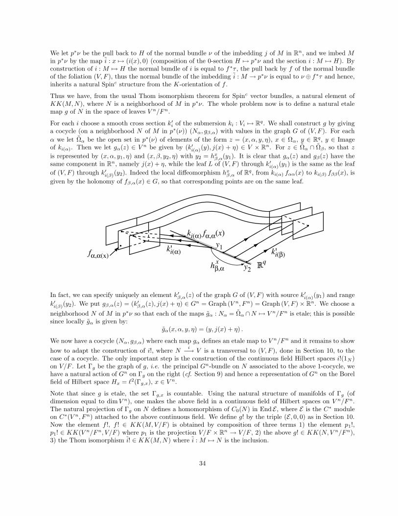
We let p∗ν be the pull back to H of the normal bundle ν of the imbedding j of M in Rn, and we imbed Min p∗ν by the map i : x 7→ (i(x), 0) (composition of the 0-section H 7→ p∗ν and the section i : M 7→ H). Byconstruction of i : M 7→ H the normal bundle of i is equal to f ∗τ , the pull back by f of the normal bundleof the foliation (V, F ), thus the normal bundle of the imbedding i : M → p∗ν is equal to ν ⊕ f∗τ and hence,inherits a natural Spinc structure from the K-orientation of f .

Thus we have, from the usual Thom isomorphism theorem for Spinc vector bundles, a natural element ofKK(M,N), where N is a neighborhood of M in p∗ν. The whole problem now is to define a natural etalemap g of N in the space of leaves V n/Fn.

For each i choose a smooth cross section k′i of the submersion ki : Vi 7→ Rq. We shall construct g by givinga cocycle (on a neighborhood N of M in p∗(ν)) (Nα, gβ,α) with values in the graph G of (V, F ). For each

α we let Ωα be the open set in p∗(ν) of elements of the form z = (x, α, y, η), x ∈ Ωα, y ∈ Rq, y ∈ Imageof ki(α). Then we let gα(z) ∈ V n be given by (k′i(α)(y), j(x) + η) ∈ V × Rn. For z ∈ Ωα ∩ Ωβ , so that z

is represented by (x, α, y1, η) and (x, β, y2, η) with y2 = hxβ,α(y1). It is clear that gα(z) and gβ(z) have the

same component in Rn, namely j(x) + η, while the leaf L of (V, F ) through k′i(α)(y1) is the same as the leaf

of (V, F ) through k′i(β)(y2). Indeed the local diffeomorphism hxβ,α of Rq , from ki(α) fαα(x) to ki(β) fββ(x), is

given by the holonomy of fβ,α(x) ∈ G, so that corresponding points are on the same leaf.

In fact, we can specify uniquely an element k′β,α(z) of the graph G of (V, F ) with source k′i(α)(y1) and range

k′i(β)(y2). We put gβ,α(z) = (k′β,α(z), j(x) + η) ∈ Gn = Graph (V n, Fn) = Graph (V, F ) × Rn. We choose a

neighborhood N of M in p∗ν so that each of the maps gα : Nα = Ωα ∩N 7→ V n/Fn is etale; this is possiblesince locally gα is given by:

gα(x, α, y, η) = (y, j(x) + η) .

We now have a cocycle (Nα, gβ,α) where each map gα defines an etale map to V n/Fn and it remains to show

how to adapt the construction of i!, where Ni

−→ V is a transversal to (V, F ), done in Section 10, to thecase of a cocycle. The only important step is the construction of the continuous field Hilbert spaces i!(1N )on V/F . Let Γg be the graph of g, i.e. the principal Gn-bundle on N associated to the above 1-cocycle, wehave a natural action of Gn on Γg on the right (cf. Section 9) and hence a representation of Gn on the Borelfield of Hilbert space Hx = `2(Γg,x), x ∈ V n.

Note that since g is etale, the set Γg,x is countable. Using the natural structure of manifolds of Γg (ofdimension equal to dimV n), one makes the above field in a continuous field of Hilbert spaces on V n/Fn.The natural projection of Γg on N defines a homomorphism of C0(N) in End E , where E is the C∗ moduleon C∗(V n, Fn) attached to the above continuous field. We define g! by the triple (E , 0, 0) as in Section 10.Now the element f !, f ! ∈ KK(M,V/F ) is obtained by composition of three terms 1) the element p1!,p1! ∈ KK(V n/Fn, V/F ) where p1 is the projection V/F × Rn → V/F , 2) the above g! ∈ KK(N, V n/Fn),3) the Thom isomorphism i! ∈ KK(M,N) where i : M 7→ N is the inclusion.

34

We of course have to check that this definition of f ! is independent of all the choices, such as the imbeddingj : M 7→ Rn made along the way. This follows from the homotopy invariance of [18] together with the proofof the invariance of the topological index in [1].

Theorem 4. Given an oriented K cycle (M,E, f) the class: f !([E]) ∈ K∗(V/F ) only depends upon thehomology class [(M,E, f)] ∈ K∗,τ (BG) of the K cycle.

We shall sketch the proof assuming that the functoriality (f1 f2)! = f2! f1! has been checked in certainspecial cases.

The compatibility with vector bundle modification (i.e. replacing M by the total space of a suitable sphere

bundle M1p

−→ M and E by a bundle E1 on M1) follows from the equality f1 = f p, p!([E1]) = [E]. Thecompatibility with bordism goes as follows, if M = ∂M1 is a boundary, the inclusion i : M 7→ D of M inthe double D of M1 is a K-oriented map, since it has a trivial one dimensional normal bundle. So if f is asmooth K oreinted map of M1 in the leaf space V/F , its restriction to M is equal to f i where f is theextension of f to the double of M1 (this extension can be assumed to be smooth). Thus if the bundle Eon M is the restriction i∗(E1) of a bundle E1 on M1, one has (f i)! [E] = f ! (i! i∗(E1)) = 0 since i! i∗ = 0.Indeed to check this, it is enough to show that i!(1M ) = 0, but i!(1M ) is the element of K1(D) defined by asmooth map ϕ : D 7→ S1 such that the 1-form on D, ω = ϕ∗(dθ), pull back of the fundamental class of S1,is equal to the element of H1(D,Z) which is dual to the cycle M and hence is equal to 0.

Remark. Using the above construction one gets a map from the analytical group K∗(V/F ) (the K-homologyof V/F ) in the sense of extension theory) to a natural geometric group K∗,τ (BG) of cocycles on BG.

12 Comparison of K∗,τ(BG) and K∗(V/F )

The most important problem in the K-theory of foliations is to be able to compute the analytical groupK∗(V/F ) in purely geometric terms. The first non trivial example is the Kronecker foliation Fθ of the twotorus V = R2/Z2 by lines of irrational slope θ. This case was settled by the remarkable breakthrough ofPimsner and Voiculescu ([22]) who exhibited an exact sequence for the K group of crossed products of aC∗ algebra A by an automorphism α ∈ Aut (A). Their result was then extended in [10], [13] to the case ofcrossed products by the real line R where it takes an extremely simple form, extending the classical Thomisomorphism. This step allows to compute K∗(V/F ) whenever the foliation F comes from a free action of asolvable simply connected Lie group H by diffeomorphisms of V .

In Section 9 we introduce the geometric groupK∗,τ (BG) which is quite easy to compute in concrete examples,moreover in Section 11 we defined a natural map µ from the geometric group to the analytical group. Themain problem can now be stated in precise terms:

Problem. Show that the map µ : K∗,τ(BG) 7→ K∗(V/F ) is always an isomorphism.

The easiest case is when the foliation (V, F ) comes from a submersion p : V 7→ B, then the classifyingspace BG with bundle τ is homotopic to B with its tangent bundle TB, so that the oriented K-homologygroup K∗,τ (BG) is naturally isomorphic to K∗(B), which in turn is obviously equal to the analytical groupK∗(V/F ).

The next important case is when the foliation (V, F ) comes from a free action by diffeomorphisms of thesimply connected solvable Lie group H . Then the classifying space BG is homotopic to the ambient manifoldV , so that (up to a shift of mod 2 degree depending on the parity of dimH) the geometric group K∗,τ (BG) isnaturally isomorphic to K∗(V ). Now by [10], exactly the same result holds for the analytical group K∗(V/F )and one has:

Theorem 5. Let (V, F ) be the foliation coming from a free action14 on V of the solvable simply connectedLie group H then the map µ : K∗,τ (BG) 7→ K∗(V/F ) is an isomorphism.

14The important point is that the graph G of (V, F ) is equal to V × H, this may occur even if the action is not free.

35

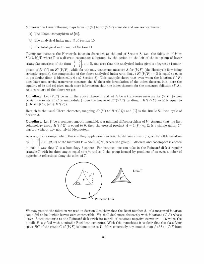
Moreover the three following maps from K∗(V ) to K∗(V/F ) coincide and are isomorphisms:

a) The Thom isomorphism of [10].

b) The analytical index map `! of Section 10.

c) The totological index map of Section 11.

Taking for instance the Horocycle foliation discussed at the end of Section 8, i.e. the foliation of V =SL (2,R)/Γ where Γ is a discrete cocompact subgroup, by the action on the left of the subgroup of lower

triangular matrices of the form

[

1 0t 1

]

, t ∈ R, one sees that the analytical index gives a (degree 1) isomor-

phism of K∗(V ) on K∗(V/F ), while for the only transverse measure Λ for (V, F ) (the Horocycle flow beingstrongly ergodic), the composition of the above analytical index with dimΛ : K∗(V/F ) 7→ R is equal to 0, soin particular dimΛ is identically 0 (cf. Section 8). This example shows that even when the foliation (V, F )does have non trivial transverse measure, the K-theoretic formulation of the index theorem (i.e. here theequality of b) and c)) gives much more information than the index theorem for the measured foliation (F,Λ).As a corollary of the above we get:

Corollary. Let (V, F ) be as in the above theorem, and let Λ be a transverse measure for (V, F ) (a nontrivial one exists iff H is unimodular) then the image of K∗(V/F ) by dimΛ : K∗(V/F ) 7→ R is equal to〈ch (E), [C]〉, [E] ∈ K∗(V ).

Here ch is the usual Chern character, mapping K∗(V ) to H∗(V,Q) and [C] is the Ruelle-Sullivan cycle ofSection 3.

Corollary. Let V be a compact smooth manifold, ϕ a minimal diffeomorphism of V . Assume that the firstcohomology group H1(V,Z) is equal to 0, then the crossed product A = C(V ) oϕ Z, is a simple unital C∗

algebra without any non trivial idempotent.

As a very nice example where this corollary applies one can take the diffeomorphism ϕ given by left translation

by

[

1 01 1

]

∈ SL (2,R) of the manifold V = SL (2,R)/Γ, where the group Γ, discrete and cocompact is chosen

in such a way that V is a homology 3-sphere. For instance one can take in the Poincare disk a regulartriangle T with its three angles equal to π/4 and as Γ the group formed by products of an even number ofhyperbolic reflections along the sides of T .

We now pass to the foliation we used in Section 3 to show that the Betti number β1 of a measured foliationcould fail to be 0 while leaves were contractible. We shall deal more abstractly with foliations (V, F ) whoseleaves L are isometric to the Poincare disk (with its metric of constant negative curvature −1), when thebundle F is gifted with a suitable Euclidean structure. With this hypothesis it is clear that the classifyingspace BG of the graph G of (V, F ) is homotopic to V . More concretely any smooth map f : M 7→ V/F from

36

a manifold to the space of leaves V/F can be lifted to V using a partition of unity on M and the hyperbolicbarycenter for n-tuples of points on the same leaf.

Thus the geometric group K∗,τ (BG) coincides with K∗(V ) and a special case of the general problem is thefollowing:

Problem. With the above hypothesis, show that the analytical index map `! : K∗(V ) 7→ K∗(V/F ) is anisomorphism.

What we shall do here is to construct an element δ of KK(V/F, V ) = KK(C∗(V, F ), C(V )) which satisfies`! δ idV where idV ∈ KK(V, V ) is the element associated to the identity map. Thus the index mapassociated to δ, which goes from K∗(V/F ) to K∗(V ), is a right inverse of `!, so that we know that `! isinjective. The next step would be to show that with the other construction of `! made in Section 11, onehas δ `! = idC∗(V,F ). This would show at the same time that the two constructions of `! do coincide andthat `! is an isomorphism. We have not however yet checked carefully this important step.

Construction of δ. In our context, F is a 2-dimensional oriented real vector bundle on V , it thus has anatural Spinc structure, and we let S = S(F ) be the corresponding complex vector bundle of spinors on Vwith its natural spitting as S = S+ ⊕ S−. For each X ∈ Fx, ξ ∈ S+

x we let c(X) ξ ∈ S−x be the Clifford

product of ξ by X .

Since δ ∈ KK(C∗(V, F ), C(V )), it is described by a C∗ module over C(V ), i.e. a continuous field (Hx)x∈V ofHilbert spaces over V . We put Hx = L2(Gx)⊗Sx, where Gx = γ ∈ G, s(γ) = x (G is the graph of (V, F )).As each leaf L of (V, F ) is simply connected, there is no holonomy and the graph G is Hausdorff, whichshows that the field (L2(Gx))x∈V of Hilbert spaces is continuous. Now for each x the representation πx ofC∗(V, F ) in L2(Gx) (cf. Section 5) defines uniquely a representation π±

x of C∗(V, F ) in H±x = L2(Gx) ⊗ S±

x

such that:π±

x (f)(ξ1 ⊗ ξ2) = πx(f) ξ1 ⊗ ξ2 ∀ f ∈ C∗(V, F ) .

In this way we get a homomorphism π± of C∗(V, F ) in the algebra of endomorphisms of H±. We now definean homomorphism ∆ of H+ to H−, for each x ∈ V , ∆x : H+

x 7→ H−x is given by the equality:

(∆x ξ)(γ) = c (ϕ(γ)′) ξ(γ) ∀ ξ ∈ L2(Gx, Sx) .

Here ϕ(γ) for γ ∈ Gx stands for the vector in Fx whose exponential is equal to y = r(γ), and the ′ meansthat for ‖ϕ(γ)‖ > 1 it has been replaced by ‖ϕ(γ)‖−1 ϕ(γ).

For f ∈ C∞c (G,Ω1/2) and each x ∈ V , π±

x (f) is a smoothing operator in L2(Gx)⊗Sx, and since γ 7→ ‖ϕ(γ)‖is a proper map from Gx to R+ it follows that with f as above the following operators are compact:

π+x (f)(∆∗

x ∆x − 1) , π−x (f)(∆x ∆∗

x − 1) .

Also, as, given ε > 0, C > 0, there exists a compact subset K of Gx such that for γ1, γ2 ∈ Gx\K,d(γ1, γ2) 5 C one has ‖ϕ′(γ1) − ϕ′(γ2)‖ 5 ε, we get that ∆x intertwines, modulo compact operators, therepresentations π±

x of C∗(V, F ).

One checks in this way that the triple (H+, H−,∆) defines an element of the Kasparov group KK(V/F, V ).

Proof of `! δ = idV . We shall reduce this check to the classical Thom isomorphism for the vector bundleF over V using the homotopy invariance of KK as in [13]. If one tries to compute directly `! δ thedifficulty is the following: one gets as a continuous field of Hilbert spaces on V : the field L2(Gx, r

∗(S))⊗Sx,but the action of C(V ) on each fiber is highly non trivial, it is given by multiplication by h r for anyh ∈ C(V ). The aim of the homotopy we are going to use is to transform this action of C(V ) on the fiber inthe multiplication by h(x), ∀h ∈ C(V ). The following construction extends the idea of [13], our first versionof this homotopy was using a parameter ~ → 0 in the pseudodifferential calculus of [7]. The present form isdue to G. Skandalis.

37

We shall construct a continuous field (Aλ)λ∈[0,1] of C∗ algebras and continuous families αλ, βλ of elements,αλ ∈ KK(Aλ, C(V )), βλ ∈ KK(C(V ), Aλ) such that for λ = 1, A1 = C∗(V, F ), α1 = δ, β1 = `! whilefor λ = 0, A0 = C0(F

∗) (where F ∗ is the total space of the dual bundle of F ) and α0 ∈ KK(F ∗, V ),β0 ∈ KK(V, F ∗) are given by the classical Thom isomorphism for the bundle F ∗. The most convenientdescription of Aλ is as the C∗ algebra of a groupoid Gλ and we shall just give the construction of thecontinuous family Gλ, the construction of the corresponding C∗ algebra Aλ can be done as in Section 5 (see

also [24] for the general theory). For each λ one has G(0)λ = V and the underlying topological space is the

total space of the bundle F . For λ = 0, the source and range maps s0, r0 are equal to the projection of Fon its base and the groupoid structure of F is the obvious group structure on each fiber Fx. For λ 6= 0, thegroupoid structure of Gλ is determined by the source and range maps sλ, rλ given by:

sλ(X) = x ∀X ∈ Fx

rλ(X) = expx(λX) ∈ leaf of x in V

where the exponential is taken in the leaf of x.

It is clear that for λ 6= 0, Gλ is isomorphic to G. The continuity of this family at λ = 0 should be clear fromthe following picture:

To describe βλ ∈ KK(C(V ), Aλ), we consider as in Section 10 3), the representation of Gλ in the Borel fieldof Hilbert spaces L2(Gλ,x, r

∗λ(S)) given by right translations. This representation defines a C∗ module Eλ

over Aλ, which for λ = 0, corresponds to the action by translations of Fx on each L2(Fx)⊗Sx. Each h ∈ C(V )defines an endomorphism of Eλ, as a multiplication operator by the function h rλ on each L2(Gλ,x, r

∗λ(S)).

Finally exactly as in Section 10 3), we define a right invariant family Dλx of pseudodifferential operators of

order 0, Dλx acting on Gλ,x from the bundle r∗λ(S+) to r∗λ(S−) and with principal symbol given by Clifford

multiplication. For λ = 0 we obtain a translation invariant operator, which is most easily described, usingFourier transform, as the operator from L2(F ∗

x )⊗S+x to L2(F ∗

x )⊗S−x given by Clifford multiplication by ξ′,

ξ ∈ F ∗x . To describe αλ ∈ KK(Aλ, C(V )), we just have to introduce the parameter λ in the construction of

δ given above. By homotopy invariance the check that `! δ = idV is reduced to β0 α0 = idV which ishandled by [18].

13 Non commutative differential geometry and transversal elliptic

theory

In the construction of the Thom isomorphismK0(A) ' K1(AoαR) for C∗ dynamical R-systems (A,R, α) 15,the crucial lemma is the following:

15A is a C∗ algebra on which the real line R acts by automorphisms (αt)t∈R.

38

Lemma. Given any orthoprojection e ∈ Proj (A), there exists an equivalent orthoprojection e′ ∈ Proj (A)and an outer equivalent action α′ of R on A, such that α′

t(e′) = e′, ∀ t ∈ R.

Though the proof of this lemma is rather trivial, it does not work for actions of R2, and what we want toexplain first is how trying the proof for actions of R2 one is led to the notion of curvature, and one can thenexhibit a non trivial obstruction.

In the case of R the proof goes as follows: 1) One replaces e by an equivalent e′ ∈ Proj (A), where e′ isnow in the domain of the derivation δ, δ(x) = lim

t7→0

1t (αt(x) − x) which defines the action of R. One does

this by first smoothing e (i.e. replacing e by αf (e) =∫

f(t)αt(e) dt where f ∈ C∞c (R) and then replacing

αf (e) by its support. Of course all this works equally well for actions of R2. 2) Letting H be the unboundedmultiplier of the crossed product A oα R such that δ(x) = Hx − xH , ∀x ∈ A one replaces the off diagonalterms e′H(1 − e′) and (1 − e′)He′ of H by 0. In other words one defines:

H ′ =

[

H11 00 H22

]

= e′He′ + (1 − e′)H(1 − e′) .

Let us pass to the case of R2. We let δ1, δ2 be the unbounded derivations of A associated to the generatorsX1, X2 of the Lie algebra of R2 and H1, H2 be the corresponding unbounded multipliers of the crossedproduct Aoα R2.

We may from step 1) above assume that e is smooth, i.e. that the map t 7→ αt(e) is C∞. What we wantis to modify H1, H2 to make them commute with e. As above, the obvious thing to do is to replace Hj byH ′

j = eHe+ (1− e)H(1− e) for j = 1, 2. The problem however, is that now H ′1 and H ′

2 no longer commute:

blocks of commuting matrices do not necessarily commute. Thus H ′1, H

′2 no longer define an action of R2.

So this method fails, and we shall now analyse why, by interpreting the commutator of eH1 e and eH2 e asthe curvature of a connection.

Recalling the correspondence between projections and finite projective modules we put:

Definition. Let E∞ be a finite projective module over A∞ = x ∈ A, t 7→ αt(x) is of class C∞. Then aconnection ∇ on E∞ is a pair of linear maps ∇1,∇2 : E∞ 7→ E∞ such that:

∇j(ξ x) = (∇j ξ)x+ ξ δj(x) ∀ ξ ∈ E∞ , x ∈ A∞ .

In the above situation the equality E∞ = eA∞ defines a (right) finite projective module over A∞, and thefollowing equalities define a special connection: the Grassmannian connection, on E∞:

∇j ξ = e δj(ξ) ∀ ξ ∈ eA∞ , j = 1, 2 .

Since δj(ξ) = Hj ξ − ξ Hj with the above notations, we see that ∇j(ξ) = (eHj e) ξ − ξ Hj and that:

(∇1∇2 −∇2∇1) ξ = [eH1 e, eH2 e] ξ .

Now quite generally we have:

Lemma. a) For any connection ∇ on E∞, the map θ = ∇1∇2 −∇2∇1 of E∞ in itself, is an endomorphism:θ(ξ x) = θ(ξ)x, ∀ ξ ∈ E∞ , x ∈ A∞ so θ ∈ End (E∞).

b) Let ∇′j = ∇j + Γj be antoher connection, Γj ∈ End(E∞), then one has the equality:

θ′ − θ = ∂1 Γ2 − ∂2 Γ1 + [Γ1,Γ2] where: (∂j X) ξ = ∇j(X ξ) −X(∇j ξ)

for any X ∈ End E∞.

39

Proof. a)

(∇1∇2 −∇2∇1)(ξ x) = ∇1(∇2 ξ)x+ ξ δ2(x) −∇2((∇1 ξ)x+ ξ δ1(x)) = (∇1∇2 ξ)x− (∇2∇1 ξ)x .

b)

(∇′1∇

′2 −∇′

2∇′1) ξ = ∇′

1(∇2 ξ + Γ2 ξ) −∇′2(∇1 ξ + Γ1 ξ)

= ∇1(∇2 ξ + Γ2 ξ) + Γ1(∇2 ξ + Γ2 ξ) −∇2(∇1 ξ + Γ1 ξ) − Γ2(∇1 ξ + Γ1 ξ)

= (∇1∇2 −∇2∇1) ξ + ∇1(Γ2 ξ) − Γ2(∇1 ξ) −∇2(Γ1 ξ) + Γ1∇2 ξ + [Γ1,Γ2] ξ .

Now one easily checks that the maps ∂j of End E∞ in itself are derivations, the commutator ∂1∂2 − ∂2∂1

being the inner derivation implemented by θ.

To extract from the above lemma an actual obstruction to our initial problem we shall assume that the C∗

algebra A is gifted with a trace τ , τ(1) = 1 which is invariant under the automorphisms αt. The invariantwill be the trace of the curvature θ (up to a normalization factor 2πi), as the trace is defined on A not onEndA∞, one first has to extend it but this is easy. For instance if E∞ = eA∞ then EndE∞ = eA∞ e andone just takes the restriction of τ . We let τE be the extension of τ to E .

Theorem 6. The scalar c1(E) = (2πi)−1 τE(θ) is independent of the choice of connection, it depends onlyon the class [E ] ∈ K0(A) and on the outer equivalence class of the action α.

Proof. Since τ is α-invariant one easily checks that τE(∂jX) = 0, j = 1, 2, X ∈ EndE∞. Thus theabove lemma makes clear that (2πi)−1 τE(∇1∇2 − ∇2∇1) is independent of the choice of the connection∇. Next, if two finite projective modules E∞

1 , E∞2 on A∞ have isomorphic images E1, E2 as modules over

A : Ej = E∞j ⊗A∞ A, they are isomorphic. As obviously: c1(E ⊕ E ′) = c1(E) + c1(E

′) for any pair E , E ′, itis clear that c1 is a map from K0(A) to R. Using the two by two matrix trick one gets easily that c1(E)depends only upon the outer equivalence class of the action α. Q.E.D.

Coming back to the case E∞ = eA∞ with e ∈ Proj (A∞), one gets the formula:

c1(e) = (2πi)−1 τ (e [δ1(e), δ2(e)]) .

So, in fact, if one can find a projection e′ ∼ e and an outer equivalent action α′ such that just one of theδ′j(e

′) is 0, one gets the vanishing of c1(e). Thus it remains to show that this obstruction is non trivial, toexhibit an example where c1(e) 6= 0.

Our example will be the irrational rotation algebra Aθ, generated by two unitaries U, V satisfying the relationV U = ei2πθ UV where θ /∈ Q.

We shall consider Aθ as the crossed product of C(S1) by the irrational rotation of angle θ and write itsgeneric element as a sum

∑

an,m Un V m =∑

fm V m where fm ∈ C(S1) admits the an,m ∈ C as Fouriercoefficients. There are two commuting derivations δ1, δ2 of Aθ which define an action α of R2 on Aθ and aregiven by δ1(

∑

fm V m) =∑

f ′m V m (where f ′

m is the ordinary derivative of the periodic function fm), whileδ2(

∑

fm V m) =∑

(2πim) fm V m. In the U, V notation the two formulas are of course similar.

We note that though it is very difficult to give the conditions on the numerical coefficients an,m ∈ C whichmake

∑

an,m Un V m an element of Aθ (it is already difficult to decide when∑

an Un defines an element of

C(S1)) it is very easy to characterize elements of A∞θ = x ∈ Aθ , t 7→ αt(x) is C∞ = ∩Domain δk1

1 δk2

2 .

Lemma. A∞θ =

∑

an,m Un V m, (an,m) is a sequence with rapid decay.

Proof. The equality τ(∑

an,mUn V m) = a0,0 defines a trace on Aθ, the finiteness of τ(x∗ x) shows that for∑

an,mUn V m ∈ Aθ the sequence (an,m) is `2. This makes it clear that if∑

an,m Un V m ∈ A∞θ one has

|nk mk′

an,m| 7→ 0 as n,m 7→ ∞ for any k, k′. Conversely, if (an,m) is of rapid decay, one has∑

an,mUn V m

because the sequence is `1, so obviously then, one has∑

an,mUn V m ∈ A∞θ . Q.E.D.

40

Of course to have a chance to get c1(e) 6= 0, we need a non trivial projection e ∈ ProjAθ. We shall usethe construction due to R. Powers and M. Rieffel: the projection e is of the form ([25]) (here (V f V ∗)(s) =f(s− θ), ∀ s) e = V ∗ g + f + g V where f, g ∈ C∞(S1) have graphs as given in the following picture:

So f is equal to 0 on [0, a] and [b + θ, 1], to 1 on [b, a + θ] and for s ∈ [a, b] one has f(s) + f(s + θ) = 1.While g is equal to 0 except on [a + θ, b + θ] where g = (f − f 2)1/2. We then have to compute c1(e) =(2πi)−1 τ(e [δ1(e), δ2(e)]). Here τ(

∑

fm V m) =∫

f0(t) dt and δ1, δ2 are as given above, so the computation

is duable and gives: 12πi [δ1(e), δ2(e)] = V ∗(g f ′ − g f

′ θ) + 2((g g′)−θ − g g′) + (g f ′ − g f′ θ)V where for

h ∈ C(S1), hθ is the translate of h by θ. In the product 12iπ e [δ1(e), δ2(e)] the term which is independent of

V is given by:g(f ′ − f

′ θ) + 2f((g g′)−θ − g g′) + (g2(f ′ − f′ θ))−θ .

When we integrate this function on S1 we can delete the last ( )−θ and with u = g2, v = f − fθ we get theintegral of 2uv′ − u′v, i.e. 3

∫

uv′ = −6∫

g2f ′. Next since g = 0 outside the interval [a+ θ, b+ θ], where fvaries from 1 to 0, and g2 = f − f2 we get:

c1(e) = 6

∫ 1

0

(λ− λ2) dλ = 1 .

Thus c1(e) 6= 0 and we have shown that the obstruction to our problem can indeed be non trivial. There ishowever a very interesting observation:

Corollary. With Aθ as above, the map c1 : K0(Aθ) 7→ R maps K0 in the integers Z.

Proof. By [22], K0(Aθ) is isomorphic to Z2 and is generated by the class of the trivial projection 1 and theclass of the above projection e. Q.E.D.

The above computation proves the integrality of c1(e) but gives little understanding of the reason of theintegrality, we are at about the same stage as if we had computed the integral of the Gaussian curvature ofa Riemann surface and found 2π× integer, but without any understanding of this integer.

We shall first begin by doing the computation of c1 : K0(Aθ) → R in a much better way. Instead ofrepresenting elements of K+

0 (Aθ) by classes of projections like e, we shall represent them by classes of finiteprojective modules over A∞

θ . Now by lemma 100, A∞θ is very easy to describe, so one expects that the same

will be true for finite projective modules over this algebra. (In a differential geometric language, what weare doing is representing elements of K+

0 by classes of smooth vector bundles.) To realize each element ofK+

0 (Aθ) as a finite projective module over A∞θ we note that Aθ is stably isomorphic to the C∗ algebra of

the Kronecker foliation Fθ, dx = θ dy of the two torus V = R2/Z2.

41

Then each closed transversal N to (V, Fθ) determines canonically a finite projective module over Aθ. Choos-ing the smooth transversal given by the closed geodesic Np,q; p, q relatively prime integers, one gets a finiteprojective module E∞

p,q over A∞θ which we now describe. The total space of E∞

p,q is the sum of q copies of theSchwartz space S(R), so we consider an element ξ of E∞

p,q as a function of two variables, one real variables ∈ R and one variable h ∈ Z/q. The action of the two generators U and V of A∞

θ is now defined as follows:

(ξ · V )(s, h) = ξ(s− ε, h+ 1) where ε =p

q− θ

(ξ · f)(s, h) = ξ(s, h) f(s+ (p/q)h)

where f is a periodic function: f ∈ C∞(R/Z), and U is the function U(s) = exp(2πis).

One checks the compatibility of this action with the equality V U = e2πiθ UV , and if θ /∈ Q one can showthat E∞

p,q is now a finite projective module over A∞θ .

Lemma. The operators (∇1 ξ)(s, h) = dds ξ(s, h) and (∇2 ξ)(s, h) = 2πis/ε ξ(s, h), ε = p

q − θ define aconnection on the finite projective module E∞

p,q .

Proof. One checks that ∇1(ξV ) = (∇1 ξ)V , ∇1(ξf) = (∇1 ξ) f + ξf ′ and that ∇2(ξV ) = (∇2 ξ)V + 2πi ξV ,∇2(ξf) = (∇2 ξ) f , ∀ ξ ∈ E∞

p,q , f ∈ C∞(S1). Q.E.D.

It follows now that the endomorphism of E∞p,q given by the curvature of this connection, is a multiple of the

identity operator:1

2πi(∇1 ∇2 −∇2 ∇1) =

1

εid =

1

p/q − θid .

Thus this connection has constant curvature, whose value is the irrational number (p/q − θ)−1. But thedimension (in the sense of Murray and von Neumann) of the finite projective module E∞

p,q is also irrational,

it is given by the transverse measure of the closed geodesic Np,q , i.e. dim(E∞p,q) =

∫ 1

0 |(pdt− θqdt)| = |p− θq|.

So the computation of c1(E∞p,q) is now straightforward, c1(E

∞p,q) = constant value of the curvature × dim E∞

p,q =(

1p/q−θ

)

|p− qθ| = ±q.

In this way we get a much better and convincing proof of the integrability of c1. In classical differentialgeometry most integrability results, such as the integrability of (2π−1)

∫

Gaussian curvature, are corollaries

42

of the Atiyah-Singer index theorem, the left hand side Index D being obviously an integer. In our context theintegrability of c1 is also a corollary of an index theorem. Instead of stating it in general we shall specializeto the above situation where the role of the algebra C∞(X) of smooth functions on the manifold X is playedby the (highly non commutative) algebra A∞

θ . We shall consider differential operators from the “bundle”E∞(0,1) to itself, and of the form:

D =∑

aα,β ∇α1 ∇β

2 aα,β ∈ EndE∞(0,1) .

Here, since p = 0, q = 1, the space E∞(0,1) is identical with the Schwartz space S(R) and ∇1 is ordinary

differentiation, ∇2 is 2πiθ × multiplication by the variable. The operators aα,β are arbitrary endomorphisms

of E∞(0,1), the two basic endomorphisms being the multiplication by the periodic function exp

(

2πiθ s

)

and thetranslation of 1. Thus typically D is an operator like:

(Df)(s) = f ′(s) + s(h−1(s) f(s− 1) + h0(s) f(s) + h1(s) f(s+ 1))

with hi periodic of period θ. The order n of D =∑

aα,β ∇α1 ∇β

2 is defined as the supremum of α + β and

its principal symbol σD(ξ) for ξ = (ξ1, ξ2) ∈ R2 is the endomorphism∑

α+β=n

aα,β ξα1 ξ

β2 of E∞

(0,1). D is called

elliptic iff σD(ξ) is invertible for any ξ 6= 0. Restricting ξ to ‖ξ‖ = 1, one thus gets a loop of invertibleelements of End (E∞

(0,1)) and hence by Bott periodicity an element of K0 of this algebra. The meaning of

c1(σD) should then be clear.

Theorem 7. Let D be an elliptic operator of the above form. Then the difference differential equation:Df = 0 has a finite dimensional space of solutions f ∈ S(R) and IndexD = dim KerD−dimKerD∗ is equalto the scalar c1(σD).

Thus we see that from C∗ algebra theory (the C∗ algebra being Aθ) one obtains a highly non trivialinformation about difference differential equations. This is in fact a special case (the case of the Kroneckerfoliation Fθ) of the transversal elliptic theory for foliations.

43

References

[1] M.F. Atiyah and I.M. Singer, The index of elliptic operators I, Ann. of Math. 87 (1968), 484-530.

[2] M.F. Atiyah and I.M. Singer, The index of elliptic operators IV, Ann. of Math. 93 (1971), 119-138.

[3] M.F. Atiyah, Elliptic operators, discrete groups an von Neumann algebras, Asterisque 32-33 (1976),43-72.

[4] M.F. Atiyah, R. Bott and V.K. Patodi, On the heat equation and the index theorem, Invent.Math. 19 (1973), 279-330.

[5] B. Blackadar, A simple unital projectionless C∗ algebra, Prepint University of Nevada (Reno).

[6] A. Connes, The von Neumann algebra of a foliation, Lecture Notes in Physics 80, Springer 1978,145-151.

[7] A. Connes, Sur la theorie non commutative de l’integration, Lecture Notes in Math. 725, Springer1979, 19-143.

[8] A. Connes, Feuilletages et algebres d’operateurs, Seminaire Bourbaki, fevrier 1980, 551-01.

[9] A. Connes, C∗ algebres et geometrie differentielle, C.R. Acad. Sci. Paris, tome 290 (1980).

[10] A. Connes, An analogue of the Thom isomorphism for crossed products of a C∗ algebra by an actionof R (to appear in Advances in Mathematics).

[11] J. Dixmier, Les C∗ algebres et leurs representations, 2eme edition, Paris, Gauthier Villars (1969).

[12] J. Dixmier, Les algebres d’operateurs dans l’espace hilbertien (algebres de von Neumann), 2emeedition, Paris, Gauthier Villars (1969).

[13] T. Fack and G. Skandalis, Connes’ analogue of the Thom isomorphism for the Kasparov groups(preprint).

[14] J. Feldman and C.C. Moore, Ergodic equivalence relations, cohomology and von Neumann algebrasI and II, Trans. Amer. Math. Soc. 234 (1977), 289-324 and 325-359.

[15] E.C. Gootman and J. Rosenberg, A proof of the generalized Effros-Hahn conjecture, Invent. Math.,Vol. 52, Fasc. 3 (1979), 283-298.

[16] A. Haefliger, Feuilletages sur les varietes ouvertes, Topology, Vol. 9 (1970), 183-194.

[17] A. Haefliger, Homotopy and integrability, Lecture Notes in Math. 197, Springer 1971, 133-163.

[18] G.G. Kasparov, OperatorK-functor and extensions of C∗ algebra, Izv. Akad. Nauk. SSSR, Ser. Mat.44 (1980), 571-636 (in russian).

[19] G.G. Kasparov, Hilbert C∗ modules: Theorems of Stinespring and Voiculescu (to appear in Journalof Operator Theory).

[20] B. Lawson, Foliations, Bull. Am. Math. Soc., Vol. 80, No 3 (1974), 369-418.

[21] J. Milnor and J. Stasheff, Characteristic classes, Ann. of Math. Studies, No 76, Princeton Univer-sity Press (1974).

[22] M. Pimsner and D. Voiculescu, Exact sequence for K groups and Ext groups of certain crossedproduct C∗ algebras, J. Operator Theory, Vol. 4 (1980), 93-118.

44

[23] J. Plante, Foliations with measure preserving holonomy, Ann. of Math. 102 (1975), 327-361.

[24] J. Renault, A groupoid approach to C∗ algebras, Lecture Notes in Math. 793, Springer (1980).

[25] M. Rieffel, Irrational rotation C∗ algebras, Short communications I.C.M. (1978).

[26] D. Ruelle and D. Sullivan, Currents, flows and diffeomorphisms, Topology 14 (1975), 319-327.

[27] J.L. Sauvageot, Ideaux primitifs dans les produits croises, J. Funct. Analysis, Vol. 31, No 3 (1979).

[28] I.M. Singer, Some remarks on operator theory and index theory, Lecture Notes in Math. 575, Springer(1977), 128-138.

[29] D. Sullivan, Cycles and the dynamical study of foliated manifolds, Invent. Math. 36 (1976), 225-255.

[30] E. Winkelnkemper, The graph of a foliation (preprint).

45